The two-point resistance of a cobweb with a superconducting boundary

Abstract

We consider the problem of two-point resistance on an $m\times n$ cobweb network with a superconducting boundary, which is topologically equivalent to a geographic globe. We deduce a concise formula for the resistance between any two nodes on the globe using a method of direct summation pioneered by one of us [Z. Z. Tan, et al, J. Phys. A 46, 195202 (2013)]. This method contrasts the Laplacian matrix approach which is difficult to apply to the geometry of a globe. Our analysis gives the result directly as a single summation.

Key words: $m\times n$ cobweb; superconducting boundary, two-point resistance; matrix equation.

PACS numbers: 84.30.Bv, 01.55.+b, 02.10.Yn, 05.50+q

I 1. Introduction

A classic problem in electric circuit theory first studied by Kirchhoff kirch more than 160 years ago is the computation of resistances in resistor networks. Kirchhoff formulated the problem in terms of the Laplacian matrix of the network and also noted that the Laplacian also generates spanning trees. For the explicit computation of two-point resistances, Venezian venezian in 1994 considered the resistance between two arbitrary nodes using the method of superposition. In 2000 Cserti cserti evaluated the two-point resistance using the lattice Green’s function. Their studies are confined to regular lattices of infinite size.

In 2004, one of us wu formulated a different approach and derived an expression for the two-point resistance in arbitrary finite and infinite lattices in terms of the eigenvalues and eigenvectors of the Laplacian matrix. The Laplacian analysis has also been extended to impedance networks after a slight modification of the formulation of tzengwu . We shall refer to these methods as the Laplacian approach. Applications of the Laplacian approach require a complete knowledge of the eigenvalues and eigenvectors of the Laplacian straightforward to obtain for regular lattices. But it is generally difficult to solve the eigenvalue problem for non-regular networks such as a cobweb.

The cobweb is a two-dimensional cylindrical network plus the insertion of an additional node connected to every node on one of the 2 boundaries. An example of the cobweb is shown in the left panel of Fig. 1. In 2013 Tan, Zhou and Yang tzy2013 proposed a conjecture, the TZY conjecture, on the resistance between 2 nodes on the cobweb. It is then difficult to adopt the Laplacian approach directly to the problem due to the special geometry of the cobweb. However, by modifying the method slightly to take care of the special cobweb geometry, Izmailian, Kennna and Wu (IKW) succeeded in establishing the TZY conjecture using a modified Laplacian approach ikw .

In this paper we consider the cobweb network with a superconducting boundary. The superconducting boundary of the cobweb shrinks the boundary into one point resulting in a network of the shape of a ball, or a globe, shown in the right panel of Fig. 1. An $m\times n$ cobweb network of $m$ rows and $n$ columns with a superconducting boundary is then equivalent to a globe with $m-1$ latitudes and $n$ longitudes. The example of $m=6,n=12$ is shown in Fig. 1. Since there are 2 poles on a globe, both the Laplacian and the IKW modified Laplacian approaches are difficult to apply.

On the other hand, studies of the resistance problem had been carried out independently by Tan and co-workers along a different route, which we shall refer to as the method of direct evaluation tzy2013 ; tan ; tanzhouluo13 ; tanchen13 . The direct method is useful in cases when there exists a special node such as a pole of the globe and the center of the cobweb, connected to all other nodes along lines such as the longitudes of a globe. This special connectivity makes it possible to compute the resistance between 2 nodes by computing separately their relative potentials with respect to the special node. One thus circumvents the need of diagonalizing a non-regular Laplacian matrix. The direct method of computing resistances was pioneered by one of us tan and has been applied successively to the cobweb network for specific values of $m$ up to $m=4$ tzy2013 ; tan ; tanzhouluo13 ; tanchen13 , It has also been used recently to compute the resistances in a fan network essamtanwu . In this paper we apply the direct method to the globe problem.

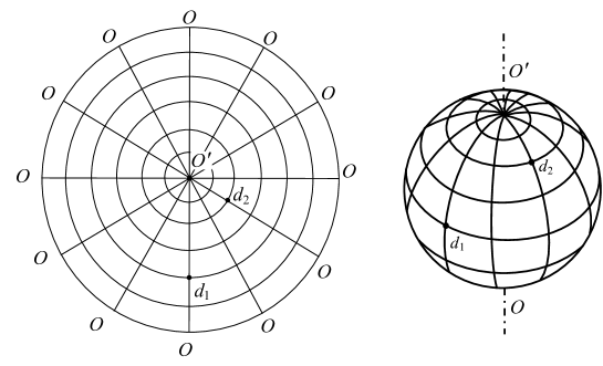
Figure 1: A $6\times 12$ cobweb network with a superconducting boundary and the equivalent globe with 5 latitudes and 12 longitudes. Bonds in longitude and latitude directions represent, respectively, resistors $r_{0}$ and $r$. The cobweb center is the north pole $O^{\prime}$, and the boundary contracts into south pole denoted by $O$.

II 2. The equivalent resistance - the main result

Consider the globe with $n$ longitudes and $m-1$ latitudes shown in Fig. 1. Bonds in longitude and latitude directions have respective resistance $r_{0}$ and $r$ and let the south pole $O$ be the origin of coordinates. Define variable $L_{i}$, and for later uses $\lambda_{i},{\bar{\lambda}}_{i}$ by

$$\lambda_{i}\equiv e^{2L_{i}} = 1+h-h\cos\theta_{i}+\sqrt{(1+h-h\cos\theta_{i})^{2}-1}$$

$${\bar{\lambda}}_{i}\equiv e^{-2L_{i}} = 1+h-h\cos\theta_{i}-\sqrt{(1+h-h\cos\theta_{i})^{2}-1}$$

$$\cosh 2L_{i} = 1+h-h\cos\theta_{i}$$ (1)

where

$$h=r/r_{0},\quad\theta_{i}={(i-1)\pi}/{m},\qquad i=1,2,...,m.$$

We find the resistance between the two nodes $d_{1}=\{1,y_{1}\}$ and $d_{2}=\{x+1,y_{2}\}$, where $\{x,y\}$ are coordinates, to be given by the expression

$$R_{m\times n}^{globe}(\{1,y_{1}\},\{x+1,y_{2}\})=\frac{(y_{1}-y_{2})^{2}}{mn}r_{0}$$

$$\quad+\frac{r}{m}\sum_{i=2}^{m}\frac{\cosh(nL_{i})(\sin^{2}y_{1}\theta_{i}+\sin^{2}y_{2}\theta_{i})-2\cosh[(n-2x)L_{i}]\sin(y_{1}\theta_{i})\,\sin(y_{2}\theta_{i})}{\sinh(2L_{i})\sinh(nL_{i})}.$$ (2)

Particularly, we have the special cases:

Case 1. When $d_{1}$ and $d_{2}$ are on the same longitude at $\{1,y_{1}\}$ and $\{1,y_{2}\}$, we have

$$R_{m\times n}^{long}(d_{1},d_{2})=\frac{(y_{1}-y_{2})^{2}}{mn}r_{0}+\frac{r}{m}\sum_{i=2}^{m}(\sin y_{1}\theta_{i}-\sin y_{2}\theta_{i})^{2}\bigg{[}\frac{\coth(nL_{i})}{\sinh(2L_{i})}\bigg{]}.$$ (3)

Case 2. When $d_{1}$ and $d_{2}$ are on the same latitude at $\{1,y\}$ and $\{x+1,y\}$, we have

$$R_{m\times n}^{latt}(d_{1},d_{2})=\frac{4r}{m}\sum_{i=2}^{m}\frac{\sinh(xL_{i})\sinh[(n-x)L_{i}]}{\sinh(2L_{i})\sinh(nL_{i})}\big{[}\sin^{2}(y\theta_{i})\big{]},$$ (4)

The expression (4) is invariant under $x\leftrightarrow(n-x)$ as expected.

Case 3. The resistance between a node at $\{x,y\}$ and the north pole $O^{\prime}$ is

$$R_{m\times n}(\{x,y\},O^{\prime})=\frac{(m-y)^{2}}{mn}r_{0}+\frac{r}{m}\sum_{i=2}^{m}\sin^{2}(y\theta_{i})\bigg{[}\frac{\coth(nL_{i})}{\sinh(2L_{i})}\bigg{]}.$$ (5)

Case 4. The resistance between the two poles $O$ and $O^{\prime}$ is

$$R_{m\times n}(O,O^{\prime})=mr_{0}/n.$$ (6)

III 3. Derivation of the main result (2)

III.1 3.1 Expressing the resistance in terms of longitudinal currents

To compute the resistance between two nodes $d_{1}=\{1,y_{1}\}$ and $d_{2}=\{x+1,y_{2}\}$, we inject a current $J$ into the network at $d_{1}$ and exit the current at $d_{2}$. Denote the currents in all segments of the network as shown in Fig. 2. Then by Ohm’s law the potential differences between $d_{1}$, $d_{2}$, and the north pole $O^{\prime}$ are, respectively,

$$U_{m\times n}^{globe}(d_{1},O^{\prime})=r_{0}\sum_{i=y_{1}+1}^{m}I_{1}^{(i)},\qquad U_{m\times n}^{globe}(O^{\prime},d_{2})=-r_{0}\sum_{i=y_{2}+1}^{m}I_{x+1}^{(i)},$$

where $I_{1}^{(i)}$ denotes currents along the longitude $1$, and $I_{x+1}^{(i)}$ denotes currents along the longitudinal $x+1$. It then follows from the Ohm’s law that the resistance between $d_{1}$ and $d_{2}$ is

$$R_{m\times n}^{globe}(\{1,y_{1}\},\{x+1,y_{2}\})=\frac{r_{0}}{J}\Big{[}\sum_{i=y_{1}+1}^{m}I_{1}^{(i)}-\sum_{i=y_{2}+1}^{m}I_{x+1}^{(i)}\Big{]}.$$ (7)

Therefore we need to find the longitudinal currents $I_{1}^{(i)}$ and $I_{x+1}^{(i)}$. This is the main objective of this paper.

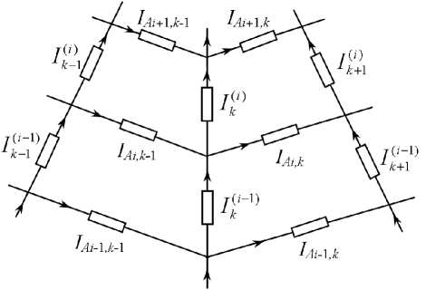
Figure 2: A segment of the globe with current directions.

III.2 3.2 Matrix equation for longitudinal currents

Analysis of the longitudinal currents is best carried out in terms of a matrix equation. Early discussions along this line are due to Tan and co-workers tzy2013 ; tan ; tanzhouluo13 ; tanchen13 . A similar analysis for a fan network has been given recently in essamtanwu .

A segment of the globe network is shown in Fig. 2 with current labeling, and we focus on the upper 2 rectangular meshes. Around the 2 meshes there are 5 longitudinal currents $I^{(i)}_{k-1},I^{(i)}_{k},I^{(i)}_{k+1},I^{(i-1)}_{k},I^{(i+1)}_{k},$ and 4 horizontal currents $I_{Ai,k}$. The potential across each current segment is either $I_{k}^{(i)}r_{0}$ or $I_{Ai,k}r$. The Kirchhoff law says that the sum of the potentials around any closed loop is equal to zero. Apply this to the outer perimeter of the two meshes, this gives a equation relating the 4 horizontal currents. Furthermore, the sum of all currents at a node must be zero. Applying this Kirchhoff rule to the upper two consecutive nodes on the longitude $k$, one obtains 2 more equations relating the 4 horizontal currents. However, it can be seen from Fig. 2 that the 4 horizontal currents enter all 3 equations only in the combination of $\Im_{1}=I_{Ai+1,k-1}-I_{Ai+1,k}$ and $\Im_{2}=I_{Ai,k-1}-I_{Ai,k}$. Thus one can eliminate $\Im_{1}$ and $\Im_{2}$ from the 3 equations. This gives the relation

$$I^{(i)}_{k+1}=-I^{(i)}_{k-1}+2(1+h)I^{(i)}_{k}-hI^{(i+1)}_{k}-hI^{(i-1)}_{k}$$ (8)

connecting the 5 longitudinal currents. After taking into account of modifications at $i=1,m$ essamtanwu , (8) can be written in a matrix form

$${\bf I}_{k+1}={\bf A}_{m}{\bf I}_{k}-{\bf I}_{k-1},\qquad$$ (9)

where ${\bf A}_{m}$ and ${\bf I}_{k}$ are

$${\bf A}_{m}=\left({\begin{array}[]{cccccc}{{2+h}}&{{-h}}&{{0}}&0&{\cdots}&{{0}}\\ {{-h}}&{{2(1+h)}}&{{-h}}&0&{\cdots}&{\cdots}\\ {\vdots}&{\ddots}&{\ddots}&\ddots&{\ddots}&{\vdots}\\ {{0}}&{\cdots}&0&{{-h}}&{{2(1+h)}}&{{-h}}\\ {{0}}&{\cdots}&{{0}}&0&{{-h}}&{{2+h}}\\ \end{array}}\right),\qquad{\bf I}_{k}=\left({\begin{array}[]{cccccc}I_{k}^{(1)}\\ I_{k}^{(2)}\\ {\vdots}\\ I_{k}^{(m-1)}\\ I_{k}^{(m)}\\ \end{array}}\right).$$ (20)

It is understood that we have the cyclic condition

$${\bf I}_{0}={\bf I}_{n},\qquad{\bf I}_{n+1}={\bf I}_{1}.$$ (21)

We consider the solution of (9) in the next section.

III.3 3.3 General solution of the matrix equation

In this section we consider the solution of (9) in the absence of an injected current, namely, $J=0$.

The eigenvalues $t_{i},\,i=1,2,...,m$ of ${\bf A}_{m}$ are the $m$ solutions of the equation

$${\rm det}\Big{|}{\bf A}_{m}-t\ {\bf{\bar{I}}_{m}}\Big{|}=0,$$ (22)

where ${\bf{\bar{I}}}_{m}$ is the $m\times m$ identity matrix. Since ${\bf A}_{m}$ is Hermitian it can be diagonalized by a similarity transformation to yield

$${\bf P}_{m}\,{\bf A}_{m}\,({\bf P}_{m})^{-1}={\bf\Lambda}_{m}$$ (23)

where ${\bf\Lambda}_{m}$ is a diagonal matrix with eigenvalues $t_{i}$ of ${\bf A}_{m}$ in the diagonal, and column vectors of $({\bf P}_{m})^{-1}$ are eigenvectors of ${\bf A}_{m}$.

It can be verified that we have

$${\bf P}_{m}=\left({\begin{array}[]{cccc}{1/\sqrt{2}}&{1/\sqrt{2}}&{\cdots}&{1/\sqrt{2}}\\ {\cos(1-\frac{1}{2})\theta_{2}}&{\cos(2-\frac{1}{2})\theta_{2}}&{\cdots}&{\cos(m-\frac{1}{2})\theta_{2}}\\ {\vdots}&{\vdots}&{\ddots}&{\vdots}\\ {\cos(1-\frac{1}{2})\theta_{m}}&{\cos(2-\frac{1}{2})\theta_{m}}&{\cdots}&{\cos(m-\frac{1}{2})\theta_{m}}\\ \end{array}}\right),$$ (28)

$$({\bf P}_{m})^{-1}=\frac{2}{m}\left({\begin{array}[]{cccc}{1/\sqrt{2}}&{\cos(1-\frac{1}{2})\theta_{2}}&{\cdots}&{\cos(1-\frac{1}{2})\theta_{m}}\\ {1/\sqrt{2}}&{\cos(2-\frac{1}{2})\theta_{2}}&{\cdots}&{\cos(2-\frac{1}{2})\theta_{m}}\\ {\vdots}&{\vdots}&{\ddots}&{\vdots}\\ {1/\sqrt{2}}&{\cos(m-\frac{1}{2})\theta_{2}}&{\cdots}&{\cos(m-\frac{1}{2})\theta_{m}}\\ \end{array}}\right),$$ (33)

where $\theta_{i}={(i-1)\pi}/{m}$,

$$t_{i} = 2(1+h)-2h\cos\theta_{i}=\lambda_{i}+\bar{\lambda}_{i}$$ (34)

$$= 2\cosh(2L_{i}),\quad\qquad\quad i=1,2,3,\cdots,m,$$

where we have made use of (1).

Apply ${\bf P}_{m}$ on the left of (9) and write

$${\bf X}_{k}\equiv{\bf P}_{m}{\bf I}_{k},\quad{\rm or}\quad{\bf I}_{k}=({\bf P}_{m})^{-1}{\bf X}_{k}.$$ (35)

After making use of (23), we obtain the equation

$${\bf X}_{k+1}={\bf\Lambda}_{m}{\bf X}_{k}-{\bf X}_{k-1}.$$ (36)

Let the $i$-th element of the column vector ${\bf X}_{k}$ be $X_{k}^{(i)}$. Then (36) gives

$$X_{k+1}^{(i)}=t_{i}X_{k}^{(i)}-X_{k-1}^{(i)},\quad i=1,2,...,m,$$ (37)

which is a set of recurrence relations for $X_{k}^{(i)}$.

For $i=1$, the solution of (37), which we shall make use later, is particularly simply. Since $\theta_{1}=0$ and $L_{1}=0$, we have $t_{1}=2$. Then (37) becomes

$$X_{k+1}^{(1)}=2X_{k}^{(1)}-X_{k-1}^{(1)},\quad k=1,2,...,n-1,$$ (38)

which together with the cyclic condition $X_{0}^{(1)}=X_{n}^{(1)}$ is a set of $n-1$ linear relations for $n$ unknowns $X_{k}^{(1)},k=1,2,...,n$, which is insufficient. But other than the trivial solution $X_{k}^{(1)}=0$ which is useless, we have also the obvious solution that all $X_{k}^{(1)}$’s are equal, namely,

$$X_{1}^{(1)}=X_{2}^{(1)}=\cdots=X_{n}^{(1)}.$$ (39)

For $i>1$, the recurrence relation (37) can be solved by the method of generating function. Define generating function

$$G(s)=\sum_{k=1}^{\infty}X_{k}^{(i)}s^{k}.$$ (40)

Multiply (37) by $s^{k}$ and sum both sides of the equation from $k=1$ to $k=\infty$. This yields

$$\frac{1}{s}\Big{[}G(s)-X_{1}^{(i)}s-X_{2}^{(i)}s^{2}\Big{]}=t_{i}\Big{[}G(s)-X_{1}^{(i)}s\Big{]}-s\,G(s)$$

from which we solve for $G(s)$, obtaining

$$G(s)=\frac{X_{1}^{(i)}s+\big{(}X_{2}^{(i)}-t_{i}X_{1}^{(i)}\big{)}s^{2}}{1-t_{i}s+s^{2}}.$$ (41)

Partial fraction (41) by using $1-t_{i}s+s^{2}=(1-\lambda_{i}s)(1-{\bar{\lambda}}_{i}s)$ where $\lambda_{i}$ and ${\bar{\lambda}}_{i}$ are defined in (1). This gives

$$\frac{1}{1-t_{i}s+s^{2}}=\frac{1}{\lambda_{i}-{\bar{\lambda}}_{i}}\bigg{(}\frac{\lambda_{i}}{1-\lambda_{i}s}-\frac{\bar{\lambda}_{i}}{1-{\bar{\lambda}}_{i}s}\bigg{)},$$

which we substitute into (41). Expand the right-hand side of (41) into a series in  $s$   by making use of $(1-z)^{-1}=1+z+z^{2}+\cdots$, and compare both sides term by term. We obtain after making use of the identity $F_{k}^{(i)}-t_{i}F_{k-1}^{(i)}=-F_{k-2}^{(i)}$ the solution of $X_{k}^{(i)}$ in terms of a given initial condition of $X_{1}^{(i)}$ and $X_{2}^{(i)}$,

$$X_{k}^{(i)}=X_{2}^{(i)}F_{k-1}^{(i)}-X_{1}^{(i)}F_{k-2}^{(i)},\quad\quad i>1,\quad k\geq 1,$$ (42)

where

$$F_{k}^{(i)}=\frac{\lambda_{i}^{k}-{\bar{\lambda}}_{i}^{k}}{\lambda_{i}-{\bar{\lambda}}_{i}}=\frac{\sinh(2kL_{i})}{\sinh(2L_{i})}.$$ (43)

In a similar fashion by considering the generating function (40) with a summation over k from $k=u+1$ to $\infty$ with a given initial condition of $X_{u+2}^{(i)}$ and $X_{u+1}^{(i)}$, where $u\geq 0$ is arbitrary, we obtain the solution

$$X_{k}^{(i)}=X_{u+2}^{(i)}F_{k-u-1}^{(i)}-X_{u+1}^{(i)}F_{k-u-2}^{(i)},\quad i>1,\quad u\geq 0,\ \quad k\geq u+1.$$ (44)

Note that (44) reduces to (42) when $u=0$.

III.4 3.4 Boundary conditions with input and output currents

While either (42) or (44) serves to determine ${\bf I}_{k}$ when there is no external current injected to the network, to compute the resistance between nodes $d_{1}=d_{1}(1,y_{1})$ and $d_{2}=d_{2}(x+1,y_{2})$ we need to inject current $J$ at $d_{1}$ and exit the current at $d_{2}$. Then (42) holds only for $1\leq k\leq x+1$. For $k$ in the range of $x+1\leq k\leq n+1$, however, we need to use (44) with $u=x$. Thus the injection of $J$ at $d_{1}(1,y_{1})$ and the exit of $J$ at $d_{2}=d_{2}(x+1,y_{2})$ specialize (9) for $k=1$ and $k=x+1$ to

$${\bf I}_{2} = {\bf A}_{m}{\bf I}_{1}-{\bf I}_{n}-J{\bf H}_{1},$$ (45)

$${\bf I}_{x+2} = {\bf A}_{m}{\bf I}_{x+1}-{\bf I}_{x}-J{\bf H}_{2},$$ (46)

where we have made use of the cyclic condition ${\bf I}_{0}={\bf I}_{n}$, ${\bf H}_{1}$ and ${\bf H}_{2}$ are column matrices with elements

$$(H_{1})_{i} = h(-\delta_{i,y_{1}}+\delta_{i,y_{1}+1}),$$

$$(H_{2})_{i} = h(\delta_{i,y_{2}}-\delta_{i,y_{2}+1}),$$

or, equivalently,

$${\bf H_{1}} = [\overbrace{0,\cdots 0,-h,h}^{\mathrm{from}~{}0\mathrm{th}~{}\mathrm{to}~{}(y_{1}+1)\mathrm{th}},0,\cdots,0\ ]^{T},$$

$${\bf H_{2}} = [\overbrace{0,\cdots 0,h,-h}^{\mathrm{from}~{}0\mathrm{th}~{}\mathrm{to}~{}(y_{2}+1)\mathrm{th}},0,\cdots,0]^{T},$$

where $[\ ]^{T}$ denote matrix transposes.

Applying ${\bf P}_{m}$ to (45) and (46) on the left, we are led to

$${\bf X}_{2} = {\bf\Lambda}_{m}{\bf X}_{1}-{\bf X}_{n}-hJ{\bf D_{1}},$$ (47)

$${\bf X}_{x+2} = {\bf\Lambda}_{m}{\bf X}_{x+1}-{\bf X}_{x}-hJ{\bf D_{2}},$$ (48)

where  $h{\bf D}_{1}={\bf P}_{m}{\bf H}_{1},\ h{\bf D}_{2}={\bf P}_{m}{\bf H}_{2}$, or equivalently,

$${\bf D_{1}} = [\zeta_{1,1},\zeta_{1,2},\cdots,\zeta_{1,i},\cdots,\zeta_{1,m-1},\zeta_{1,m}]^{T}$$

$$\zeta_{1,i} = P_{y_{1},i}-P_{y_{1}+1,i}=-\cos\bigg{(}y_{1}-\frac{1}{2}\bigg{)}\theta_{i}+\cos\bigg{(}y_{1}+\frac{1}{2}\bigg{)}\theta_{i}$$ (49)

$$= -2\sin(y_{1}\theta_{i})\sin(\theta_{i}/2),$$

$${\bf D_{2}} = [\zeta_{2,1},\zeta_{2,2},\cdots,\zeta_{2,i},\cdots,\zeta_{2,m-1},\zeta_{2,m}]^{T}$$

$$\zeta_{2,i} = P_{y_{2},i}-P_{y_{2}+1,i}=\cos\bigg{(}y_{2}-\frac{1}{2}\bigg{)}\theta_{i}-\cos\bigg{(}y_{2}+\frac{1}{2}\bigg{)}\theta_{i}$$ (50)

$$= 2\sin\big{(}y_{2}\theta_{i})\sin(\theta_{i}/2).$$

Explicitly, (47) and (48) read

$$X^{(i)}_{2}=t_{i}X_{1}^{(i)}-X^{(i)}_{n}-hJ\zeta_{1,i},$$ (51)

$$X^{(i)}_{x+2}=t_{i}X^{(i)}_{x+1}-X^{(i)}_{x}-hJ\zeta_{2,i},$$ (52)

where $t_{i}=2\cosh 2L_{i}$.

To determine the initial conditions $X_{1}^{(i)},X_{x+1}^{(i)}$ needed in our resistance calculation (7), we set $k=x,x+1$ in (42), $u=x$ and $k=n,n+1$ in (44) and making use of the cyclic condition (21) $X_{n+1}^{(i)}=X_{1}^{(i)}$. Together with (51) and (52) this gives 6 equations relating the 6 unknowns $X_{1}^{(i)},X_{2}^{(i)},X_{n}^{(i)},X_{x}^{(i)},X_{x+1}^{(i)},X_{x+2}^{(i)}$,

$$\quad\left({\begin{array}[]{cccccc}F^{(i)}_{x-2}&-F^{(i)}_{x-1}&0&1&0&0\\ F^{(i)}_{x-1}&-F^{(i)}_{x}&0&0&1&0\\ t_{i}&-1&-1&0&0&0\\ 0&0&1&0&F^{(i)}_{n-x-2}&-F^{(i)}_{n-x-1}\\ 1&0&0&0&F^{(i)}_{n-x-1}&-F^{(i)}_{n-x}\\ 0&0&0&-1&t_{i}&-1\\ \end{array}}\right)\left({\begin{array}[]{cccccc}X_{1}^{(i)}\\ X_{2}^{(i)}\\ X_{n}^{(i)}\\ X_{x}^{(i)}\\ X_{x+1}^{(i)}\\ X_{x+2}^{(i)}\\ \end{array}}\right)=\left({\begin{array}[]{cccccc}0\\ 0\\ hJ\zeta_{1,i}\\ 0\\ 0\\ hJ\zeta_{2,i}\end{array}}\right),\quad i>1,$$ (71)

where $t_{i}=2\cosh(2L_{i})$ and $F_{k}^{(i)}=\sinh(2kL_{i})/\sinh(2L_{i})$.

Solving (71), we obtain after some algebra and reduction the 2 solutions needed in our resistance calculation (7),

$$X_{1}^{(i)} = \frac{(F_{n-x}^{(i)}+F_{x}^{(i)})\zeta_{2,i}+F_{n}^{(i)}\zeta_{1,i}}{4\sinh^{2}nL_{i}}(hJ)$$ (72)

$$= hJ\bigg{[}\frac{(F_{n-x}^{(i)}+F_{x}^{(i)})\sin(y_{2}\theta_{i})-F_{n}^{(i)}\sin(y_{1}\theta_{i})}{2\sinh^{2}nL_{i}}\bigg{]}\sin(\theta_{i}/2),\quad i>1,$$

$$X_{x+1}^{(i)} = \frac{(F_{n-x}^{(i)}+F_{x}^{(i)})\zeta_{1,i}+F_{n}^{(i)}\zeta_{2,i}}{4\sinh^{2}nL_{i}}(hJ)$$ (73)

$$= hJ\bigg{[}\frac{-(F_{n-x}^{(i)}+F_{x}^{(i)})\sin(y_{1}\theta_{i})+F_{n}^{(i)}\sin(y_{2}\theta_{i})}{2\sinh^{2}nL_{i}}\bigg{]}\sin(\theta_{i}/2),\quad i>1.$$

For completeness, we also list the other 4 solutions of (71) although they are not needed in our calculation,

$$X_{2}^{(i)} = {\frac{{(F_{x-1}^{(i)}+F_{n-x+1}^{(i)})\zeta_{2,i}+(F_{1}^{(i)}+F_{n-1}^{(i)})\zeta_{1,i}}}{{4\sinh^{2}nL_{i}}}}(hJ),$$

$$X_{n}^{(i)} = \frac{{(F_{x+1}^{(i)}+F_{n-x-1}^{(i)})\zeta_{2,i}+(F_{1}^{(i)}+F_{n-1}^{(i)})\zeta_{1,i}}}{{4\sinh^{2}nL_{i}}}(hJ),$$

$$X_{x}^{(i)} = {\frac{{(F_{x-1}^{(i)}+F_{n-x+1}^{(i)})\zeta_{1,i}+(F_{1}^{(i)}+F_{n-1}^{(i)})\zeta_{2,i}}}{{4\sinh^{2}nL_{i}}}}(hJ),$$

$$X_{x+2}^{(i)} = {\frac{{(F_{1}^{(i)}+F_{n-1}^{(i)})\zeta_{2,i}+(F_{x+1}^{(i)}+F_{n-x-1}^{(i)})\zeta_{1,i}}}{{4\sinh^{2}nL_{i}}}}(hJ).$$

Solutions (72) and (73) are useful for $i>1$. For $i=1$ (72) and (73) give the trivial solutions $X_{1}^{(1)}=X_{x+1}^{(1)}=0$. But when $i=1$ we have $\zeta_{1,i}=\zeta_{2,i}=0$ so (51) and (52) reduce to (38). Then using the same argument leading to (39), we again obtain $X_{1}^{(1)}=X_{2}^{(1)}=\cdots=X_{n}^{(1)}$. This permits us to write

$$X_{1}^{(1)}=\frac{1}{n}\sum_{k=1}^{n}X_{k}^{(1)}=\frac{1}{n}\sum_{k=1}^{n}\sum_{j=1}^{m}\big{[}({\bf P_{m}})_{1j}I_{k}^{(j)}\big{]}=\frac{1}{\sqrt{2}\,n}\sum_{i=1}^{m}\sum_{k=1}^{n}I_{k}^{(i)}$$ (74)

where we have made use of $({\bf P_{m}})_{1j}=1/\sqrt{2}$.

The summations in (74) are taken over all longitudinal current segments on the globe. Since the current $J$ flows from a node at latitude $y_{1}$ to a node at latitude $y_{2}$, by conservation of current the summation over segments at a given latitude $i$ must yield $J$ for $y_{1}<i\leq y_{2}$ and zero otherwise, namely,

$$\sum_{k=1}^{n}I_{k}^{(i)} = J,\qquad\quad y_{1}<i<y_{2}+1$$ (75)

$$= 0,\qquad\quad{\rm otherwise},$$

so (74) gives the simple result

$$X_{1}^{(1)}=\frac{J}{\sqrt{2}\,n}(y_{2}-y_{1}).$$ (76)

III.5 3.5 The equivalent resistance

We are now in a position to evaluate the resistance (7). From (35) we have

$$I_{1}^{(i)}=\sum_{j=1}^{m}[({\bf P}_{m})^{-1}]_{ij}X_{1}^{(j)}.$$

Using $({\bf P}_{m})^{-1}$ given by (33) with $({\bf P}_{m})^{-1})_{i1}=\sqrt{2}/m$ for all $i$, it is clear that the $j=1$ term in the summation needs to be singled out. This gives

$$I_{1}^{(i)}=\ \frac{\sqrt{2}}{m}X_{1}^{(1)}+\frac{2}{m}\sum_{j=2}^{m}X_{1}^{(j)}\cos\bigg{(}i-\frac{1}{2}\bigg{)}\theta_{j}$$ (77)

and thus

$$\sum_{i=y_{1}+1}^{m}I_{1}^{(i)}=\frac{\sqrt{2}}{m}(m-y_{1})X_{1}^{(1)}-\frac{1}{m}\sum_{j=2}^{m}X_{1}^{(j)}\bigg{[}\frac{\sin(y_{1}\theta_{j})}{\sin(\frac{1}{2}\theta_{j})}\bigg{]},$$ (78)

where we have used the formula

$$\sum_{i=y+1}^{m}\cos\bigg{(}i-\frac{1}{2}\bigg{)}\theta_{j}=-\bigg{[}\frac{\sin(y\theta_{j})}{2\sin(\frac{1}{2}\theta_{j})}\bigg{]}$$ (79)

which can be established by using the identity $\sum_{k=1}^{n}\cos(k-\frac{1}{2})x=\sin(nx)/2\sin(x/2)$ gr .

Substituting (76) into (78), we obtain

$$\sum_{i=y_{1}+1}^{m}I_{1}^{(i)}=\frac{J}{mn}(m-y_{1})(y_{2}-y_{1})-\frac{1}{m}\sum_{j=2}^{m}X_{1}^{(j)}\bigg{[}\frac{\sin(y_{1}\theta_{j})}{\sin(\frac{1}{2}\theta_{j})}\bigg{]}.$$ (80)

Similarly, we also obtain

$$\sum_{i=y_{2}+1}^{m}I_{x+1}^{(i)}=\frac{J}{mn}(m-y_{2})(y_{2}-y_{1})-\frac{1}{m}\sum_{j=2}^{m}X_{x+1}^{(j)}\bigg{[}\frac{\sin(y_{2}\theta_{j})}{\sin(\frac{1}{2}\theta_{j})}\bigg{]}.$$ (81)

Substituting (80) and (81) into (7), we obtain

$$R_{m\times n}^{globe}(d_{1},d_{2})=\frac{r_{0}}{m}\bigg{[}\frac{(y_{2}-y_{1})^{2}}{n}+\frac{1}{J}\sum_{i=2}^{m}\frac{X_{x+1}^{(i)}\sin(y_{2}\theta_{i})-X_{1}^{(i)}\sin(y_{1}\theta_{i})}{\sin(\frac{1}{2}\theta_{i})}\bigg{]}.$$ (82)

Finally, we obtain our main result (2) by further substituting $X_{1}^{(i)}$ and $X_{x+1}^{(i)}$ from (72) and (73) into (82).

III.6 3.6 Special cases

Case 1: When $d_{1}=\{1,y_{1}\}$ and $d_{2}=\{1,y_{2}\}$ are on the same longitude, we take $x=0$, (2) reduces immediately to (3).

Case 2: When $d_{1}=\{1,y\}$ and $d_{2}=\{x+1,y\}$ are on the same latitude $y$, (2) immediately reduces to (4).

Case 3: The resistance between a node at $\{x,y\}$ and the north pole $O^{\prime}$ is obtained by setting $y_{1}=y,\,y_{2}=m$ in (3). This gives (5).

Case 4: The resistance between the two poles is obtained by setting both $y_{1}=0,\,y_{2}=m$ in (3). This gives $R_{m\times n}(O,O^{\prime})=mr_{0}/n$. This result can also be deduced by considering $R_{m\times n}(O,O^{\prime})$ as connecting $n$ linear chains of resistance $mr_{0}$ each in parallel, since by symmetry there are no currents in the horizontal direction.

III.7 3.7 A simple example

As an example, we apply (2) to a $2\times 4$ globe shown in Fig. 3. In this case the summation in (2) has only one term $i=2$ with $\theta_{2}=\pi/2,m=2,\ n=4$, and

$$\cosh(2L_{2})=1+h,\quad\cosh(4L_{2})=1+4h+2h^{2},$$

$$\sinh(2L_{2})\sinh(4L_{2})=2h(1+h)(2+h).\qquad$$

For the resistance between $O$ and $A$, we use (5) with $y=1$ and obtain

$$R_{2\times 4}(O,A) = \frac{1}{8}r_{0}+\bigg{(}\frac{r}{2}\bigg{)}{\frac{{\cosh(4L_{i})}\sin^{2}\theta_{2}}{{\sinh(2L_{i})\sinh(4L_{i})}}}=\frac{4+11h+5h^{2}}{8(1+h)(2+h)}r_{0}.$$

For the resistance between $A$ and $B$, we use (4) with $x=y=1$, and obtain

$$R_{2\times 4}(A,B) = \frac{{\cosh 4L_{i}-\cosh 2L_{i}}}{{\sinh(2L_{i})\sinh(4L_{i})}}(r\sin^{2}\theta_{2})=\frac{h(3+2h)}{2(1+h)(2+h)}r_{0}.$$

For the resistance between $A$ and $C$, we use (4) with $x=2,y=1$, and obtain

$$R_{2\times 4}(A,C) = {\frac{{\sinh^{2}(2L_{i})}}{{\sinh(2L_{i})\sinh(4L_{i})}}}(2r\sin^{2}\theta_{2})=\frac{h}{1+h}r_{0}.$$

The resistance between $O$ and $O^{\prime}$ is given by (6) directly as

$$R_{2\times 4}(O,O^{\prime})=\frac{1}{2}r_{0}.$$

Here $A,B,C$ denote nodes shown in Fig. 3 and we have used $r=hr_{0}$. We have verified these results by carrying out explicit calculations.

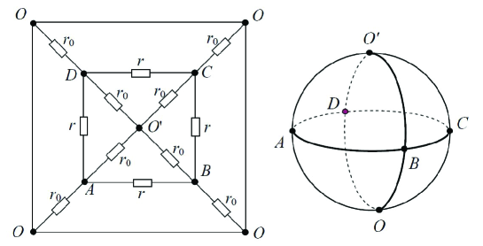
Figure 3: A $2\times 4$ globe and the associated cobweb network with a superconducting boundary. Node $O$ denotes the contraction of the superconducting boundary and is the coordinate center.

IV 4. Summary and discussion

In 2004 Wu wu established a theorem which computes the equivalent resistance between two nodes in a resistor network using the Laplacian approach. For the $m\times n$ network the results are in the form of a double summation. Additional work is required to reduce this to a single summation.

An alternative direct approach of computing resistances had been developed by Tan and co-workers tzy2013 ; tan ; tanzhouluo13 ; tanchen13 which, when applied to the cobweb and globe networks, gives the result in terms of a single summation, thus offering a direct and somewhat simpler approach. The direct method has been used by the present authors essamtanwu to deduce the 2-point resistance in a fan network. Here we use the direct method to compute resistances in a globe network, which is equivalent to the cobweb with a superconducting boundary. Our main result is (2) which gives the resistance between any two nodes of the globe. Various special cases of the main result are also presented.

It is instructive to comment on why the Laplacian method is not used. While it is tempting to use the Laplacian method and formulate the globe problem as a cobweb with zero resistances along its boundary, but since elements of the Laplacian are conductances, the inverse of resistances which is infinite, this is not easily done. It is simpler and easier to use the direct approach.

Finally, we remark that the direct method of computing resistance can be extended to impedance networks, since the Ohm’s law based on which the method is formulated is applicable to impedances. This is advantageous than the Laplacian method which needs to be modified when dealing with impedance networks as the Laplacian matrix is generally complex and non-Hermitian requiring special considerations tzengwu .

References

References

(1)
Kirchhoff G 1847 Ann. Phys. Chem.72 497
(2)
G. Venezian, Am. J. Phys. 62 1000 (1994).
(3) J. Cserti, Am. J. Phys. 68 896 (2000).
(4) F. Y. Wu, J. Phys. A: Math. Gen. 37 6653 (2004).
(5) W. J. Tzeng, F. Y. Wu, J. Phys. A: Math. Gen. 39 8579 (2006).
(6) Z. Z. Tan, L. Zhou and J. H. Yang, J. Phys. A: Math. Theor. 46 195202 (2013)
(7) N. Sh. Izmailian, R. Kenna and F.Y.Wu. J. Phys. A: Math. Theor. 47 035003(2014)
(8) Z. Z. Tan, Resistor network Models (in Chinese) Xidian University of
Science and Technology Press, Xian, China (2011).
(9) Z. Z. Tan, L. Zhou and D. F. Luo, Int. J. Circ. Theor. Appl. DOI:10.1002/cta.1943 (2013).