On the relation between sSFR and metallicity

Abstract

In this paper we present an exact general analytic expression $Z(sSFR)={y_{Z}\over\Lambda(sSFR)}+I(sSFR)$ linking the gas metallicity $Z$ to the specific star formation rate (sSFR), that validates and extends the approximate relation put forward by Lilly et al. (2013, L13), where $y_{z}$ is the yield per stellar generation, $\Lambda(sSFR)$ is the instantaneous ratio between inflow and star formation rate expressed as a function of the sSFR, and $I$ is the integral of the past enrichment history, respectively.

We then demonstrate that the instantaneous metallicity of a self-regulating system, such that its sSFR decreases with decreasing redshift, can be well approximated by the first term on the right-hand side in the above formula, which provide an upper bound to the metallicity. The metallicity is well approximated also by $Z_{L13}^{id}=Z(sSFR)={y_{Z}\over 1+\eta+sSFR/\nu}$ (L13 ideal regulator case), which provides a lower bound to the actual metallicity. We compare these approximate analytic formulae to numerical results and infer a discrepancy $<0.1$ dex in a range of metallicities ($log(Z/Z_{\odot})\in[-1.5,0]$, for $y_{z}\equiv Z_{\odot}=0.02$) and almost three orders of magnitude in the sSFR.

We explore the consequences of the L13 model on the mass-weighted metallicity in the stellar component of the galaxies. We find that the stellar average metallicity lags $\sim 0.1-0.2$ dex behind the gas-phase metallicity relation, in agreement with the data.

1 Introduction

The evolution of the metallicity in galaxies constrains the history of the gas accretion relative to the star formation, as well as the relative importance of outflows. As such it has been extensively studied at different cosmic epochs. Whilst the full stellar metallicity distribution is available only for a few selected nearby galaxies, including the Milky Way and its components, average metallicities in the stars and in the gas of star forming regions are available for many more objects at different cosmic epochs (O’Connell, 1976, Lequeux et al., 1979, Tremonti et al., 2004, Savaglio et al. 2005, Mayer et al., 2005, 2006, Erb et al. 2006, Cid Fernandes et al. 2007, Maiolino et al., 2008, Mannucci et al., 2009, Zahid, et al., 2012, Leja, et al., 2013, Gallazzi et al., 2006, Panter et al., 2008, Sommariva et al., 2010, and references therein). These observations have established that, at any redshift $z<4$, the most massive galaxies are the most metal rich in both their gas and stellar components. Moreover, at fixed mass, the gas metallicity of star forming objects decreases with increasing redshift (Erb et al., 2006, Maiolino et al., 2008, Mannucci et al., 2009, Mannucci et al., 2011 Richard et al., 2011, Yuan et al., 2013).

Among the many theoretical attempts to understand the drivers of such relations, analytical chemical evolution models appeal either to a decreasing importance of outflows (e.g. Garnett, 2002, Tremonti et al., 2004, Spitoni et al., 2010, and/or differential winds , e.g., Dalcanton, 2007, Recchi et al., 2008) or to an increase in the star formation efficiency (Dalcanton, 2007, Spitoni et all., 2010, Peeples & Shankar, 2010), a variation in the yield (via a flattening of the IMF, e.g. Koeppen et al., 2007) or an increase in the fraction of re-accreted metals (Davé et al., 2012), with galactic mass, as possible explanations. It is worth pointing out that, in many cases, these models are adopted to interpret the data at a single epoch. On the other hand, galaxy formation numerical experiments, such as cosmological simulations and semi-analytical models, despite qualitatively matching the $z\sim 0$ relation, do not reproduce its slope (e.g. Pipino et al., 2009) and generally suffer from over-predicting the metallicity of high-redshift star forming galaxies (see, e.g., the discussion in Maiolino et al., 2008, and references therein, Sakstein et al., 2011, Yates et al., 2012).

More recently, a new dimension was added to the observational picture, with studies suggesting that, globally, the gas metallicity $Z$ of $z\sim 0$ galaxies depends also on the (specific) star formation rate (SFR): at a fixed galaxy mass, higher metallicities correspond to a lower star formation activity (e.g. Ellison et al., 2008, Mannucci et al., 2010, but see e.g. Yates et al., 2012). Furthermore, there is empirical evidence suggesting the local nature of such mass-SFR-Z relation (Rosales-Ortega et al., 2012), and the question becomes as to whether the $Z=Z(M,SFR)$ relation is redshift independent; that is if high redshift galaxies populate the extrapolation of the so-called $z\sim 0$ fundamental-metallicity relation, that can either be a surface in the mass-SFR-metallicity space (Mannucci et al., 2010) or a plane (Lara-Lopez et al., 2010, 2013) out to $z\sim 2$, or even $z=3$ (when accounting for changes in the ionization parameter, Nagajima & Ouchi, 2013, Cullen et al., 2013). Such a debate is lively and far from being set (see e.g., Cresci et al., 2011, Richard, et al. 2011, Niino, 2012, Wuyts et al., 2012, Christensen et al., 2012, Stott et al., 2013, Henry et al., 2013, Troncoso et al., 2013, Zahid et al., 2013, Belli et al., 2013). However, irrespective of the final answer, it highlights the importance of fully and simultaneously addressing galaxy evolution in terms of mass-metallicity and mass-SFR relations and their evolution with redshift. It offers an independent test-bed to the above-mentioned analytic chemical evolution models and provides new constraints to the the increasing body of theoretical works (e.g. Bouché et al., 2010, Dutton et al., 2010, Lilly et al. 2013, L13, and references therein) aimed at explaining the existence and the evolution of the SFR-mass relation (e.g., Elbaz et al., 2007, Noeske et al., 2007, Daddi et al., 2007, Pannella et al., 2009, Oliver et al., 2010) and/or the cosmic run of the specific SFR (sSFR) with simple models for the galaxy growth.

In particular, L13 show that the $z<2$ evolution of the sSFR of galaxies may be controlled by the cosmological infall of gas, through the regulating action of the gas reservoir via a Schmidt (1959) linear star formation law. Such a simple model broadly explains at the same time the cosmic evolution of the sSFR (e.g. Gonzalez et al., 2010, Stark et al., 2012, and references therein) and the stellar-to-halo mass ratio (e.g., Moster et al., 2010). More importantly, the L13 model has the additional appealing property of offering an explanation both to the evolution of the gas phase metallicity and to its scatter at a given epoch by directly linking it to variations in the sSFR with just one equation. That is, the sSFR both enters as a second paramenter in setting the metallicity and gives and explanation to the epoch-invariant fundamental metallicity relation, thereby linking the epoch-dependence and the SFR-dependence of the mass-metallicity relation.

At a fixed epoch, the slope of the mass-metallicity relation is then given by the variation of both the star formation and outflow efficiencies with stellar mass (see also Calura et al., 2009). In L13, however, the instantaneous gas phase metallicity is replaced with the value derived considering the system in equilibrium (i.e. imposing $dZ/dt=0$) for both an ideal case of regulator (steady state at constant gas fraction) and a case in which the gas fraction is slowly changing.
Other analytic models do not either make explicit the sSFR dependence of metallicity (e.g. Dayal et al., 2013) or, despite their similarity to L13, adopt a different notion of “steady-state” (e.g., constant gas mass evolution, e.g., Davé et al., 2012), claiming that the temporal variation in the metallicity for a given galaxy is driven by the amount of metals ejected in the surrounding medium and then re-accreted. Also in the case of Davé et al. (2012), approximate values for the metallicity are adopted.
Given the important role of metallicity as a constraint to galaxy formation theories and the progresses in the measurement of Z, SFR and stellar masses at progressively higher redshifts, it is important to derive full analytical expressions that link the metallicity evolution to the sSFR evolution of a single galaxy for generic gas accretion and outflow histories. If correct, the above mentioned approximated formulae (e.g. L13, Davé et al., 2012) could be then re-derived from such general solutions as special cases and applied in suitable regimes of the galaxy growth.

Table 1: Input parameters

	This paper	L13	remarks
Baryonic accretion rate	$\dot{M}_{acc}$	$\Phi$	given by cosmological background
SF efficiency	$\nu$	$\epsilon$	constant (may vary with galactic mass and/or cosmic time)
Gas-to-total fraction	$\mu$	$\nu_{gas}$	-
Gas-to-star fraction	$f$	$\mu$	-
Infall rate-to-SFR ratio	$\Lambda$	$1/f_{star}$	varies with time
Outflow rate-to-SFR ratio	$\eta$	$\lambda/(1-R)$	may vary with time
Yield per stellar generation	$y_{z}$	$y$	constant
Metallicity of infalling gas	$Z_{A}$	$Z_{0}$	constant
Returned fraction	$R$	$R$	constant

The aim of this paper is thus to validate and extend the L13 relation between $Z$ and sSFR. To this end, we revisit the L13 equations, link them to analytical models of chemical evolution (Pagel & Patchett 1975; Hartwick 1976; Twarog 1980; Tinsley, 1980, Matteucci & Chiosi, 1983, Clayton, 1988, Edmunds, 1990, Koeppen & Edmunds, 1999, Matteucci 2001, Spitoni et al., 2010), and derive a more general relation in which the metallicity Z is an explicit function of the sSFR for arbitrary gas inflow and outflow histories. We then derive simplified relation for the the Closed Box Model, the steady state evolution and the L13 model as special cases of the general solution. Furthermore, we study the range of validity and the goodness of the L13 approximation by comparing these results to a direct numerical integration of the same equations as well as to the predictions of full numerical chemical evolution models, which relax some of the assumptions done to make the problem analytically tractable.

Finally, we test the predictions of the L13 model for the evolution of the mass-stellar metallicity relation with redshift in the specific L13 case and compare it to recent observations (Sommariva et al., 2012).

The L13 model and some of its equations are briefly summarized in Sec. 2 with the double aim to both set the stage, introducing the relevant physical quantities and symbols, and to link it to the standard equation of analytic chemical evolution model. In Sec. 3, general relations between gas-phase metallicity and sSFR are presented and their special cases discussed. L13 model predictions regarding the stellar average metallicity and its comparison to data are presented in Sec. 4. Finally, in Sec. 5 we summarize and discuss our main conclusions.

2 The L13 model in the framework of analytic chemical evolution

2.1 The regulation of the baryonic content in L13

L13 suggests that the average galaxy evolution can be broadly explained by very simple physics, as it is determined by the host halo accretion rate and regulated by the star formation rate $\psi$, which is directly proportional to the interstellar medium mass (the “gas reservoir”) via the star formation efficiency $\nu$ (see Table 1), that we will keep constant with time. The model also accounts for the action of SFR-related (e.g. supernova-driven) galactic winds.

Let us define $\mu$ as the gas fraction $M_{gas}/M_{tot}$, with $M_{tot}=M_{*}+M_{gas}$. This implies that the sSFR can be written as (Eq. 7 in L13):

$$sSFR=\psi/M_{*}=\nu\,M_{gas}/M_{*}=\nu{\mu\over 1-\mu}\,.$$ (1)

The system accretes gas via inflows, with a given accretion rate $\dot{M}_{acc}$. More specifically, the L13 model assumes that haloes grow according to average prescriptions given by fit to numerical simulations (e.g. Eq 3 in L13 and references therein). Baryons are accreted proportionally to the dark matter, via the universal baryon fraction. A fraction $f_{gal}$ of the accreted baryons can penetrate into the actively star forming region and be transformed into stars, as well as possibly ejected by winds.

The simplest (ideal) case of such a regulator has the feature of setting the sSFR equal to the specific baryonic accretion rate $sMIR_{B}$. L13 (c.f. their Fig. 3) further show that, for any sudden and instantaneous variation in $sMIR_{B}$, the sSFR adjusts to a value that coincides with $sMIR_{B}$ on a timescale set by the shorter between $1/\nu$ and $1/sSFR$. The sSFR tracks the $sMIR_{B}$ also if this is steadily increasing with time. Only when the variation $dsMIR_{B}/dt<0$ and occurs on a timescale which is faster than $1/\nu$, then the sSFR decrease is slower than the drop in the $sMIR_{B}$.

Our study will focus on the metallicity-sSFR dependence. Therefore we do not further discuss the dark matter host halo growth. The cycle of inflow-star formation-outflow that we discuss below pertains to the baryons within the galaxy, therefore our conclusions do not depend on the chosen $f_{gal}$ either, with the assumption that this value is not affected by, e.g., the galactic star formation rate or the outflows.

Below we briefly present the relevant equations of L13’s model set-up in a slightly different way in order to link the L13 equation and symbols to the terms that are more common in chemical evolution studies and with the aim of summarizing some of L13’s key results to the reader, setting the stage for the present study. To this purpose, in Table 1 we summarize the main physical quantities and the symbols adopted in both the present work and in L13.

2.2 Basic equations for the evolution of gas mass and metallicity

As in L13, in this paper we follow the evolution of a galaxy made of gas, assumed to be in a single phase and well mixed at any time, with initial mass $M_{gas,0}$, and stars, whose initial mass is set to zero. The evolution of the system can be studied solving an array of equations representing the conservation of the total, the gas and the metal mass in presence of source terms (infall, outflow and nucleosynthesis).

Before doing it, it is convenient to introduce the variables $\Lambda(t)$ and $\eta(t)$ , defined in order for the infall and outflow rate to be cast in terms of the SFR $\psi(t)$. Namely, the outflow rate $W(t)$ is defined as (Matteucci & Chiosi, 1983):

$$W(t)=\eta(t)(1-R)\psi(t),$$ (2)

and it is justified by the observational evidences of ubiquitous winds in star forming galaxies (e.g., Newman et al., 2012, Bordoloi et al., 2011, 2013, Weiner et al., 2005), with mass loading factors comparable to the SFR. Since the same loading factor, within the uncertainties, is observed at different redshifts in galaxies with different SFRs (c.f. Newman et al., 2012 and references therein), for a first order approximation it is reasonable to assume that $\eta\sim const$ in galaxies with SFR-driven winds. Therefore, in the following we will present both examples and special cases assuming that $\eta$ is strictly constant in time. On the other hand, in deriving the full solution $Z=Z(sSFR)$ we will let $\eta$ arbitrarily vary with either time or sSFR.

The infall rate is given by:

$$\dot{M}_{acc}=\Lambda(t)(1-R)\psi(t).$$ (3)

The term $\Lambda(t)$ was introduced and set to a constant value by Matteucci & Chiosi (1983), to make the problem tractable analytically. The same time-invariant definition (i.e. Eq. 3 with $\Lambda=const$) is adopted in many other papers in the literature. In our approach, instead, the equation above is actually inverted and solved for $\Lambda(t)$, which will provide a way for parameterize how the SFR instantaneously responds to changes in the known accretion rate. Therefore, in this case (and in L13’s formulation) $\Lambda(t)\propto{\dot{M}_{acc}\over\psi(t)}$ is a function of time and becomes the instantaneous measure of the ratio between the gas accretion rate (given by the cosmological model) and the star formation rate.

The returned fraction by stars $R$ is defined by invoking the Instantaneous Recycling Approximation (IRA, Schmidt, 1963) as:

$$R=\int_{1\,M_{\odot}}^{\infty}(m-m_{R})\phi(m)dm,$$ (4)

where $\phi(m)$ is the IMF and $m_{R}$ is the mass of the stellar remnant. The IMF is assumed constant in time. The yield per stellar generation is then defined as (Tinsley, 1980):

$$y_{Z}={1\over{1-R}}\int_{1\,M_{\odot}}^{\infty}mp_{Z,m}\phi(m)dm,$$ (5)

where $p_{Z,m}$ is the fraction of newly produced and ejected metals by a star of mass $m$. Finally, $Z_{A}$ is the metallicity of the infalling gas.

Under these assumptions and definitions, the equations that regulate the evolution of the system in L13 become exactly those used by analytical models for chemical evolution with inflows and outflows (e.g., Pagel & Patchett 1975, Hartwick 1976, Twarog 1980; Tinsley, 1980, Edmunds, 1990, Koeppen & Edmunds, 1999, Matteucci 2001, Spitoni et al., 2010):

$$\cases{{dM_{tot}\over dt}=(\Lambda(t)-\eta(t))(1-R)\psi(t)\cr\cr{dM_{gas}\over dt}=(\Lambda(t)-\eta(t)-1)(1-R)\psi(t)\cr\cr{dZ\cdot M_{gas}\over dt}=(1-R)\psi(t)[\Lambda(t)Z_{A}+y_{Z}-(\eta(t)+1)Z]}$$ (6)

with the only difference that, in L13 and in this paper, $\Lambda$ and $\eta$ may vary with time, not least as the system increases its mass. Also, both the star formation law and the accretion rate of the galaxy are specified, whereas in standard analytical chemical evolution models, it is customary to express metallicity variations as a function of $\mu$ without any explicit dependence on both SFR and $\dot{M}_{acc}$.

Combining the first two equations in the array 6, L13 (see their Eq. 12) came to the following link between $\Lambda(t)$ and sSFR:

$$\Lambda(t)=sSFR(t)/\nu+\eta(t)+1+{1\over(1-R)\nu}{dlnf\over dt}\,,$$ (7)

where $f=M_{gas}/M_{*}=sSFR/\nu$. Eq. 20 that we discuss below is a special case of this general relation.

2.3 The gas metallicity in the L13 approach

Rather than explicitly solving Eq. 6 also for the metallicity, L13 derive approximate solutions by assuming the system to be in equilibrium. That is by solving the third equation in the array 6 by imposing $dZ/dt=0$. Indeed, L13 derive two slightly different approximations for the metallicity: one that holds in the case of a ideal regulator (i.e. with the gas fraction identically constant in time), and one that holds for the more realistic non-ideal regulator (Eqs. 26 and 29 in L13). In the formalism of this paper, these two approximations become:

$$Z_{L13}^{id}\equiv{Z_{A}+y_{z}\over sSFR/\nu+\eta+1}$$ (8)

(9)

(10)

$$Z_{L13}\equiv{Z_{A}+y_{z}\over sSFR/\nu+\eta+1+{1\over(1-R)\nu}{dlnf\over dt}}={Z_{A}+y_{z}\over\Lambda(t)}\,,$$ (11)

respectively. We remind the reader that in L13 $\eta=const$. Such simple expressions for the metallicity have non-trivial consequences. In the first place, the variation in the sSFR with cosmic epoch will drive a change in the metallicity of a given “average” galaxy.

Secondly, at any given time, two galaxies with the same stellar mass may have different metallicities, according to the values of the $sSFR,\,\eta,\,\nu,\,f$ that characterize them. In the framework of this analytical model, such a difference in metallicity is caused by the different “equilibrium” gas fraction in the two galaxies (or equivalently, their sSFR, if the other terms in the denominator are smaller). That is, a mass-metallicity-SFR relation is naturally predicted by the L13 model. More quantitatively, at a given epoch, two galaxies $i=1,2$ with given stellar masses $M_{i}$ will have the ratio of their metallicities given by (assuming $Z_{A}=0,\eta=0$, ideal regulator case):

$$Z_{L13,1}/Z_{L13,2}=$$

$$=\nu_{1}M_{1}/\nu_{2}M_{2}\;(SFR_{2}+M_{2}\cdot\nu_{2})/(SFR_{1}+M_{1}\cdot\nu_{1})=$$

$$=:M_{1}/M_{2}\;SFR_{2}/SFR_{1}\,H(sSFR_{i},\nu_{i}(M_{i}))\,,$$

that is

$$Log(Z_{1}/Z_{2})=Log(M_{1}/M_{2})-Log(SFR_{1}/SFR_{2})+Log(H)\,.$$

3 The metallicity evolution

The set of equations presented in (6) with suitable initial conditions are sufficient to characterize the galaxy evolution in terms of its gas mass, gas fraction and metallicity evolution, by direct integration over time. These solutions can then be transformed into an sSFR dependence via the sSFR-$\mu$ (Eq. 1) and sSFR-$\Lambda$ (Eq. 7) relations. This will be the core and novel aspect of this paper. In particular, we will derive two versions of a more general solution of the equations which include among their terms both the L13 approximations ($Z_{L13}^{id}$, $Z_{L13}$). We will then show under which conditions and how quickly the other terms is the solutions become negligible and, thus, L13 approximations become good solutions. In the final part of this Section we will compare the full analytical solution to the approximate L13 solution, and both to numerically-derived trends, to test the range of validity and the accuracy.

3.1 General solution: $Z$ as a function of time and sSFR

Let us take a step back and start by recalling the formal general solutions for the gas and the metallicity evolution with the explicit time dependence that can be derived by the same set of three equations (6) if one leaves the accretion rate unspecified and further assumes $\eta=const$ (in analogy with previous works and L13):

$$M_{gas}=\displaystyle e^{-\nu(1-R)(1+\eta)t}\times$$ (12)

$$\times\Bigg{(}M_{gas,0}+\int_{0}^{t}\!e^{\nu(1-R)(1+\eta)t^{\prime}}\dot{M}acc(t^{\prime})\mathrm{d}t^{\prime}\Bigg{)}\,,$$ (13)

and

$$Z=\displaystyle y_{z}\nu(1-R)e^{-\nu(1-R)\,\int_{0}^{t}\!\Lambda(t^{\prime})\mathrm{d}t^{\prime}}\times$$ (14)

$$\times\int_{0}^{t}\!e^{\nu(1-R)\,\int_{0}^{t^{\prime}}\!\Lambda(t^{\prime\prime})\mathrm{d}t^{\prime\prime}}(1+{\Lambda(t^{\prime})Z_{A}(t^{\prime})\over y_{z}})\mathrm{d}t^{\prime}\,,$$ (15)

(see also Recchi et al., 2008, for the solution with $Z_{A}=0$). For simplicity, we assumed that $Z(0)=0$ and that $\nu$ and $\eta$ are constant with time. We also assumed no variations in the IMF (and hence in the yield $y_{z}$) with either time or mass. These formulae can be obtained as standard solutions of the differential equations of the array 6 in a manner that is similar to what we show in Section 3.3 (Eq. 19 onward); therefore we do not repeat the derivation here.

Assuming that $Z_{A}=const$, substituting $\Lambda(t)$ in Eq. 15 with the expression given by Eq. 7 and integrating the resulting expression by parts, it follows that:

$$Z=Z_{A}+y_{z}\nu(1-R)\Bigg{(}{1\over\nu(1-R)(1+\eta+sSFR/\nu)}+$$

$$-{e^{-\nu(1-R)\,((1+\eta)t+\int_{0}^{t}\!sSFR(t^{\prime})/\nu\mathrm{d}t^{\prime})}\over\nu(1-R)(1+\eta+sSFR(0)/\nu)}sSFR(0)/\nu+$$

$$-{(1+\eta)\,e^{-\nu(1-R)\,((1+\eta)t+\int_{0}^{t}\!sSFR(t^{\prime})/\nu\mathrm{d}t^{\prime})}\over sSFR/\nu}\times$$

$$\times\int_{0}^{t}\!{e^{\nu(1-R)\,((1+\eta)t^{\prime}+\int_{0}^{t^{\prime}}\!sSFR(t^{\prime\prime})/\nu\mathrm{d}t^{\prime\prime})}\over\nu(1-R)(1+\eta+sSFR/\nu)^{2}}{\mathrm{d}sSFR/\nu\over\mathrm{d}t^{\prime}}\mathrm{d}t^{\prime}\Bigg{)}=$$

$$=:(I_{1}-I_{2}-I_{3})\,.$$

Where

$$I_{1}\equiv Z_{L13}^{id}={Z_{A}+y_{z}\over 1+\eta+sSFR/\nu}\,.$$ (16)

Despite two terms in the addition ($I_{2},I_{3}$ - which incorporate the integral of the accretion history), have still the explicit dependence on time, we made an important step forward as we have the first term ($Z_{L13}^{id}$) depending only on the sSFR. As we will see below, $Z_{L13}^{id}$ is also a bounding value to the true metallicity. To understand the meaning of $I_{1}=Z_{L13}^{id}$ in this context, we need to look first at the following special case of the general solution: the evolution at constant gas fraction.

3.2 Special case I - Evolution at constant gas fraction

If the galaxy is constantly in an accretion-dominated regime, that is if we add the assumption that $\Lambda,\,\eta$ are both constant with time and that $\Lambda-\eta>$1, then $M_{tot}$ increases with time. The gas fraction evolves as (e.g., Eq. 9 in Recchi et al., 2008):

$$\mu=\mu_{\rm steady}+{f_{M}\over\Lambda-\eta}\,,$$ (17)

where

$$\mu_{\rm steady}={{\Lambda-\eta-1}\over{\Lambda-\eta}}\,,$$ (18)

and

$$f_{M}=M_{gas,0}/M_{tot}(t)\,.$$ (19)

Therefore, the gas fraction tends to the value given by $\mu_{\rm steady}$. This is what we refer to as steady state, namely an evolution at a constant gas fraction, whose value is set by the constant $\Lambda-\eta$. In this particular case it is trivial to combine Eqs. 1 and 18 to show that the sSFR can be expressed as:

$$sSFR/\nu=\Lambda-\eta-1\,.$$ (20)

We note that the convergence towards the asymptotic values is faster for larger $\nu$ (the shorter the star formation timescale) and/or larger $\Lambda$.

When the steady state is attained, with $\Lambda,\eta$ and the $sSFR$ constant in time, the solution for the metallicity becomes much simpler:

$$Z_{ss}^{true}=Z_{A}+\frac{y_{z}}{\Lambda}\Bigg{(}1-e^{-\nu(1-R)\Lambda t}\Bigg{)}\,$$ (21)

$$\rightarrow Z_{A}+\frac{y_{z}}{\Lambda}=Z_{A}+\frac{y_{z}}{1+\eta+sSFR/\nu}\,,$$ (22)

at times $t>1/\nu>1/(\nu(1-R)\Lambda)$.

That is, the metallicity settles to the constant value given by $Z_{L13}^{id}$. As such, the asymptotic regime for the equilibrium metallicity (i.e. when $dZ/dt=0$) is used in L13 as the value for the metallicity in the case of the ideal regulator (i.e. when the gas fraction stays constant). This result further clarifies the meaning to the $Z_{L13}^{id}$ term (Eq. 11) contributing to the metallicity in the general equation. It is in fact a “steady-state-like” term, determined by the current value of the sSFR.

We also derive another interesting result, probably overlooked in the recent literature on the sSFR evolution at high redshift. In particular, Eq. 15 implies that one can easily model a galaxy evolving at constant sSFR as the result of an accretion dominated regime where $\Lambda-\eta-1=const>1$. The results showed in this section imply that, at the same time, the metallicity would not evolve (assuming $Z_{A}=const$). Since $Z$ is observed to decrease at $z>2$, this is another reason to suspect that the sSFR is also not constant at $z>2$ (see, e.g., Stark et al., 2012).

3.3 Integrating the metallicity equation over the sSFR

One can alternatively set up the differential equation for the metallicity variation as a function of the sSFR as the time variable. With the aim to derive a very general solution, from this section onward, not only we keep considering $\Lambda$ as a function of time (and sSFR), but also we relax the assumption of $\eta=const$ with both time and sSFR. In particular, we note that Eq. 7 can be rewritten as:

$${dsSFR\over dt}=\nu(1-R)sSFR(\Lambda(t)-\eta(t)-1-sSFR/\nu)\,.$$ (23)

Combining the third equation with the second one in the array 6, one can write:

$${dZ\over dt}=(1-R)\nu[\Lambda(t)Z_{A}+y_{Z}-\Lambda(t)Z]\,.$$ (24)

Dividing Eq. 24 by Eq. 23, one can derive an expression for $dZ/dsSFR$. Some algebra then leads to the following differential equation for the metallicity:

$${dZ\over dsSFR}+F(sSFR)Z=y_{z}G(sSFR)\,,$$ (25)

where

$$G(sSFR)={1+{Z_{A}\Lambda\over y_{z}}\over sSFR/\nu(\Lambda-\eta-1-sSFR/\nu)}\,,$$ (26)

and

$$F(sSFR)={1\over{{1\over\Lambda}+{Z_{A}\over y_{z}}}}\,G(sSFR)\,.$$ (27)

This equation has the following formal solution:

$$Z=\displaystyle y_{z}e^{-\,\int_{x_{0}}^{x}\!F(x^{\prime})\mathrm{d}x^{\prime}}\int_{x_{0}}^{x}\!e^{\int_{x_{0}}^{x^{\prime}}\!F(x^{\prime\prime})\mathrm{d}x^{\prime\prime}}G(x^{\prime})\mathrm{d}x^{\prime}\,,$$ (28)

where $x=sSFR/\nu$. Integrating by parts, with the further assumption that $Z_{A}=const$, the solution can be written as:

$$Z=Z_{A}+{y_{z}\over\Lambda(x)}-y_{z}e^{-\int_{x_{0}}^{x}F(x^{\prime})dx^{\prime}}\int_{x_{0}}^{x}{e^{\int_{x_{0}}^{x^{\prime\prime}}F(x^{\prime})dx^{\prime}}\over\Lambda(x^{\prime\prime})^{2}}{d\Lambda\over dx^{\prime\prime}}dx^{\prime\prime}\,.$$ (29)

This new way to solve for the metallicity uses the sSFR itself as the time variable. This formal analytic solution is similar to Eq. 3.1, with the difference that here we make explicit the contribution by the instantaneous value of $\Lambda(t)$ and $\eta(t)$ as if it were in the steady state, that is

$$Z_{ss}^{inst}=Z_{A}+{y_{z}\over\Lambda}=$$ (30)

(31)

$$=Z_{A}+{y_{z}\over sSFR/\nu+\eta+1+{1\over(1-R)\nu}{dlnf\over dt}}\equiv Z_{L13}\,,$$ (32)

namely the value of the metallicity adopted in L13 for the “non-ideal regulator” (i.e. gas fraction slowly varying in time). The other term in the addition is the ’resistance’ to move to the new steady state, $-\tilde{I}_{2}$, given by the past chemical evolution history. With this version of the general solution for the metallicity, we made explicit the fact that $Z_{L13}$ is one of the terms that contribute to the actual metallicity of the galaxy in the general case. Eq. 23 readily tells us that, when $\tilde{I}_{2}$ is small (as in the L13 model), the evolution of galaxies can be approximated by a sequence of steady state solutions with lower equilibrium gas fractions (lower sSFR) and higher metallicities. We quantify this statement in the next section.

3.4 Special case II - Accretion rate slowly changing with time (L13)

Having derived general formulae linking the metallicity to the sSFR for arbitrary gas accretion histories (Eqs. 11 and 23), we can now discuss the L13 approximations. In order to move from the general equations discussed above to the L13 special cases we simply need to add the assumption - explicitly made in L13 - that the sSFR slowly changes in time in order to better quantify the other terms ($I_{2}$, $I_{3}$, $\tilde{I}_{2}$) in both Eqs. 11 and 23. In particular, we now discuss the case in which the sSFR slowly decreases following the cosmological decrease in $sMIR_{B}$. As a matter of fact, similar considerations can be done for a slowly increasing sSFR, driven by, e.g., an increasing accretion rate; therefore we do not further discuss this specific case and refer the reader to L13 (c.f. their Fig. 3) for some examples on how quickly the sSFR responds to changes in either direction in the accretion rate. For simplicity, we also assume that $Z_{A}=0$, since it only adds a constant offset.

For a smoothly declining accretion history it follows that:

1) As discussed in L13 (their Eq. 39) ${dlnf\over dt}$ is small, but finite and negative, hence:

$$\;{1\over sSFR/\nu+\eta+1+{1\over(1-R)\nu}{dlnf\over dt}}>{1\over sSFR/\nu+\eta+1}$$ (33)

Therefore $Z_{L13}^{id}<Z_{L13}$. Moreover:

2) $\tilde{I}_{2}>0$. Therefore $Z<Z_{L13}$.

3) Also, $I_{2}$ falls off exponentially. Therefore $I_{2}\simeq 0$, for practical purposes, whereas $-I_{3}>0$, as the time derivative of the sSFR is negative. Therefore $Z>Z_{L13}^{id}$

By combining these results together, we derive that the true value of the metallicity is always within the range $[Z_{L13}^{id},Z_{L13}]$. This shows that, for a large class of models with the sSFR slowly decreasing in time, rather simple expressions (Eqs. 16- 32) can be used to bracket the actual gas-phase metallicity. In other words, for $\dot{M}_{acc}$ decreasing with time, the true metallicity will be bound between $Z_{L13}^{id}$ (the steady-state-like metallicity set by the current value of the sSFR, the ideal regulator case in L13) and $Z_{L13}$ (the steady-state metallicity set by the current value of $\Lambda(t)$, in L13 this is the formula used when the gas fraction is allowed to vary in the non ideal regulator case).

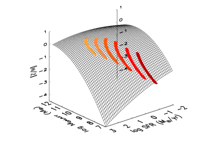
Figure 6: $z<4$ evolution of the models discussed in Figs. 3 and 4 in the three dimensional space given by star formation rate, mass and metallicity. The shaded area is the analytical formula of the fundamental metallicity relation given by Mannucci et al. (2010).

The next step is to assess the goodness of the approximation of using the steady-state(-like) metallicities (i.e. either $Z_{L13}^{id}$ or $Z_{L13}$) as an estimate of the current metallicity for these systems. This will be the topic of the next section. Here we conclude by highlighting the qualitative explanation. In the chemical evolution literature terms, the L13 smoothly evolving model is equivalent to a system in which the metallicity varies in response to a slowly changing $\Lambda(t)$. Among others, the behavior of $Z$ in the varying $\Lambda(t)$ case, has been also graphically and qualitatively discussed by Koeppen & Edmunds (1999). When, e.g., $\Lambda(t)$ slowly decreases with time, the system evolves along the locus of the steady-state solutions on the $\mu-$Z plane, moving towards lower gas fractions and higher metallicities. That is, from the steady state set by $\Lambda(t-dt)$ and $\eta(t-dt)$ to a new steady state (given by the current value of $\Lambda(t)$ and $\eta(t)$), where the new $\mu_{\rm steady}$ is lower than the old one, whereas $Z_{\rm steady}$ increases (Koeppen & Edmunds, 1999, their Figs. 5 and 6).

3.4.1 The accuracy of the L13 approximation: comparison to full analytic solutions

If one further adopts the initial condition $\mu=1$ (no stars), then $x_{0}=sSFR(0)/\nu$ diverges. Therefore we can assume $x_{0}=\infty$ in Eq. 29.

In L13 the $sSFR$ decreases with time, driven by a decrease in $\dot{M}_{acc}$. The variation is slow and at late times $|{dsSFR\over dt}|/sSFR<<1$; this implies also a very small variation in the gas fraction ($\mu$ or equivalently $f$). Therefore, there exists an epoch $t_{1}$ where $sSFR/\nu=x_{1}<<1+\eta$ and $\Lambda\simeq 1+\eta$. This implies that ${d\Lambda\over dx}\rightarrow 0$ when $t>t_{1}$ ($x<x_{1}$).

As a consequence, we can write

$$\tilde{I}_{2}=\int_{x_{0}}^{x}{e^{\int_{\infty}^{b}F(a)da}\over\Lambda(b)^{2}}{d\Lambda\over db}db\simeq\int_{\infty}^{x_{1}}{e^{\int_{\infty}^{b}F(a)da}\over\Lambda(b)^{2}}{d\Lambda\over db}db\,,$$

that is $\tilde{I}_{2}$ is effectively constant at $x<x_{1}$ (i.e. at late times).

At the same time, the exponent of the factor in front of $\tilde{I}_{2}$ grows in absolute value, therefore the second term in Eq. 23 is:

$$e^{-const/x}\times\tilde{I}_{2}\rightarrow 0$$

In this case Eq. 23 trivially reduces to:

$$Z\simeq{y_{z}\over\Lambda(x)}\equiv Z_{L13}\,.$$ (34)

Similarly, $I_{3}$ is small because it has an exponentially declining factor and in the integral we have $|{\mathrm{d}sSFR/\nu\over\mathrm{d}t^{\prime}}|<<(1+\eta+sSFR/\nu)^{2}$). We already discussed that $I_{2}$ has a fast exponential decline. Therefore also the “corrections” given by $I_{2}$ and $I_{3}$ to the metallicity in Eq. 11 are small.

To reinforce our findings, in Fig. 1 we compare the numerical integration of the metallicity (solid line) with these two limiting values (dashed - $Z_{L13}^{id}$, lower limit; dotted - $Z_{L13}$, upper limit) for a particular set of $\nu$, $y_{z}$ and given gas accretion history. For the sake of simplicity, we also arbitrarily set $y_{z}=0.02=Z_{sun}$, $\eta=0$ and $\nu=1$/Gyr.

The formula $Z=Z_{L13}^{id}={y_{z}\over 1+\eta+sSFR/\nu}$, used by L13 for the ideal regulator case (and $Z_{A}=0$) gives always an excellent approximation, departing from the numerical solution only by 0.1 dex at very late stages. It is the best approximations of the true metallicity at the highest values of the sSFR.

On the other hand, the difference $Z-Z_{L13}$ is significant in the very early phases of the evolution, when $\Lambda(t)$ and sSFR are un-correlated. This is however a consequence of our set-up. In fact, assigning an initial $\mu=1$ leads the model to evolve by consuming the gas mass initially present in a way that is independent from the inflow, as a closed box. A different initial set-up might reduce the difference between $Z_{L13}$ and the actual metallicity in these early phases. At late times, instead, in this example, $Z_{L13}$ gives a very accurate approximation of the true metallicity.

Figure 1: Evolution of the metallicity as a function of the sSFR for galaxies evolving according to the L13 model. The solid line is the evolution given by the numerical integration of Eq. 15, whereas the dashed line is the metallicity approximated as $Z\sim Z_{L13}^{id}$ (Eq. 11, see text). Finally, the dotted line gives the metallicity approximated by $Z_{L13}$ (Eq. 23).

3.5 Special case III - The Closed Box Model in terms of the sSFR

Before comparing the analytic approximate solutions to other numerical models, we mention that, in the case of a model with neither accretion nor outflows ($\Lambda=\eta=0$, Closed Box approximation, also known as the Simple Model), the relation between metallicity and sSFR trivially is:

$$Z=y_{z}ln{1+sSFR/\nu\over sSFR/\nu}\,$$ (35)

which, at early times (high sSFR), has the following approximate behavior:

$$Z\simeq y_{z}\nu/sSFR\simeq y_{z}\nu/(1+sSFR)\,$$ (36)

which is very similar to $Z_{L13}^{id}$ when $Z_{A}=\eta=0$. As the Closed Box Model well approximates the behavior of a model with $\Lambda(t)\neq 0$ at early times (high gas fraction, e.g. Koeppen & Edmunds 1999), this last equation is a good representation of the general equation behavior in the regime of high sSFRs.

Therefore, we can conclude that the sSFR, rather than $\Lambda$, seems to be the key quantity to accurately estimate the gas metallicity of the system in a variety of cases. The reasons lies in its close relation to the gas fraction $\mu$.

Also, in the Closed Box Model, the star formation has an exponential decline with timescale $\tau=\nu(1-R)$. The results in this section then provide a ready estimate for a self-consistent evolution of the metallicity and sSFR for the widely adopted exponentially decaying star formation histories.

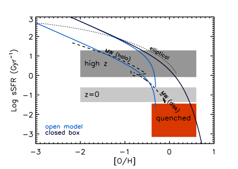
Figure 2: Evolution of the metallicity as a function of the sSFR. The dashed line is the evolution predicted by a full numerical chemical evolution model tuned to reproduce the Milky Way (MW) properties, whereas the dotted line is the prediction for a model calibrated on both local ellipticals (Pipino & Matteucci, 2004) and high redshift galaxies (Pipino et al., 2011). The solid lines give the metallicity approximated as $Z\sim Z_{L13}^{id}$ (see text) for models with accretion (blue) and closed box (black). In this illustration, $Z_{A}=\eta=0$, $y_{z}=0.01$ and $\nu$ are matched to that used in the full numerical chemical evolution models. Dark (light) grey areas give the typical values of the sSFR observed in high-(low-)redshift galaxies, whereas the red box highlights the sSFR values for quenched systems.

3.6 The accuracy of the L13 approximation: comparison to full chemical evolution models

The IRA is not a good approximation to follow a system for a long ($>1$ Gyr) time, even if we focus on the total metallicity, which is dominated by O (produced on a short timescale) and/or on metallicity inferred from O lines (among others). That is, when $\mu<<$1 and after several Gyr of evolution, the effects of metals being recycled by low mass stars cannot be ignored. We therefore further tested Eq. 3.1 against the predictions of full numerical chemical evolution models calibrated on the abundance pattern of the Milky Way and the properties of local ellipticals. We refer the reader to Pipino & Matteucci (2004), Pipino et al. (2011), and Calura et al. (2009) for a description of these models, and to Pipino et al. (2013) for their predicted sSFRs, respectively. The comparison is shown in Fig. 2, where the tracks in the metallicity-sSFR plane are show for both analytical (solid) and numerical (dashed, Milky Way -MW; dotted, elliptical) models. In the analytical models $\nu$ is matched to that used in the full numerical chemical evolution simulations. For the same reason, we set $\eta=Z_{A}=0$. The $Z\sim Z_{L13}^{id}$ approximation works well for a wide range in sSFR, becoming less accurate at late times for the case of the Milky Way as expected. The difference is however less than a factor of 2, comparable to the observational uncertainty in deriving the gas-phase metallicity. As far as elliptical galaxies are concerned, we note that the closed box approximation (solid black line) works better than the case with an infall with a long timescale (solid blue lines). This is not unexpected since these galaxies should have formed on a short timescale (e.g., Matteucci, 1994), or equivalently, at high sSFR (e.g. Pipino et al., 2013 and references therein). In the numerical models, the galactic wind prevents the star formation to occur at arbitrarily low gas fractions (hence sSFR), whereas the ideal closed box systems proceeds with $\mu\ \rightarrow\ 0$. To guide the eyes, dark (light) grey areas give the typical values of the sSFR observed in high-(low-)redshift galaxies, whereas the red box highlights the sSFR values for quenched systems at $z\sim 0$.

From this comparison, we can therefore conclude that a quasi-steady-state evolution depicted in analytic models (as in L13) must be typical of relatively low sSFR, disc galaxies, possibly representing the majority of the star forming “main sequence” at $z<2$. For these galaxies, the current metallicity is well approximated by a steady-state-like value set by the current sSFR. We suggest here that ellipticals, instead, evolve at higher sSFR for a given metallicity than spiral galaxies for a given mass, in a suggestive analogy to what happens in the [$\alpha$/Fe]-[Fe/H] plane (e.g. Fig. 4 in Matteucci & Brocato, 1990). That is, highly $alpha$-enhanced stellar populations are a distinctive feature of galaxies formed with high average sSFR, similar to those observed at $z>2$ (c.f. Pipino et al., 2013, see also discussions in Peng et al., 2010, in the context of empirical models of galaxy growth, and in Pipino et al., 2009 - their Sec. 3.2 - in the context of semi-analytical models of galaxy formation). Clearly, having adopted the IRA to make the problem analytically tractable, any abundance ratio predicted in the framework of this paper (and in L13) will be constant in time and simply equal to the ratio of the yields, unless one invokes selective inflows/outflows. Therefore, we cannot predict an analytical quantitative relation between sSFR and $\alpha/Fe$ ratio in the gas of a star forming galaxy.

We stress, however, that the “morphology” classes introduced in this section simply refer to the two typical parametrizations adopted in numerical chemical evolution simulations. Namely high $\nu$ and quick infall are needed to reproduce the chemical abundance pattern of present-day ellipticals, whereas smaller $\nu$ and longer accretion histories seem to be typical of spirals, respectively. Therefore, in the context of this paper, such “morphological” classes should be understood as useful terms for linking the L13 model (and the more general equations presented in this paper) to special cases of standard numerical models of chemical evolution. A link between the actual morphology of the galaxies and the L13 model is beyond the scope of this paper.

Figure 3: Predicted stellar metallicity distribution for arbitrary galaxy models evolving as prescribed by the L13 framework. See text for details.

Finally, one can exploit Fig. 2 as a diagnostic plot to readily estimate the star formation efficiency of a given galaxy observed at a given epoch, by simply comparing its location in the sSFR-metallicity plane with a set of model predictions at fixed yield (IMF) and varying $\nu$.

As mentioned above, the IRA does not hold at timescales comparable with those of massive stars. This would have a noticeable effect if we were dealing with the chemical abundance ratios produced by a single stellar generation. On the other hand, it is important to note that the metal return of a stellar generation does not depend on the infall/outflow history.

In the earliest phases of the galaxy evolution, when the systems is not smoothly evolving, the biggest uncertainty in the derivation of the actual gas metallicity Z is not related to the computation of the yield per se (and hence the assumption of the IRA), but probably comes from the assumption of the ISM being always homogeneous and well-mixed, as there might not be enough time for the metals to, e.g., cool down in new star forming sites or to travel a long distance. Eq. 24 will still hold on a suitably chosen local level, if one replaces the infall metallicity $Z_{A}$ with that inflowing from neighbouring regions, and considers the wind term will pollute the ISM immediately around the star forming region. On a galaxy-wide scale, a suitable convolution of such a local version applied to all star forming regions, would then give the overall metallicity evolution.

4 The metallicity in the stars of L13 galaxies

4.1 The stellar metallicity distribution

Let us start by showing the expected stellar metallicity distribution (SMD) in the framework of the L13 model, that is the fraction of stars per metallicity bin. In order to illustrate the SMDs behavior we show in Fig. 3 a sample of galaxies smoothly evolving according to L13. In this example, the galaxy final masses are in the range $10^{9-11}M_{\odot}$, and we assume that the more massive the galaxy, the higher $\nu$ (in the range 0.1-1.3/Gyr). We also assume that $Z_{A}=0$ and a formation redshift, namely when the star formation rate is switched on, of $z_{F}=10$. From the figure we can qualitatively infer an increase in the gas phase metallicity created by the variation in $\nu$ is mirrored by an increase in the average stellar metallicity. In particular, the average metallicity in the most evolved (i.e., most massive) galaxies already attained its uppermost boundary, set by the yield (e.g. Edmunds, 1990), $y_{z}=0.02$ in this illustration. The larger star formation efficiency at high masses makes the SMD rather sharply peaked around $Z\sim y_{z}$. Lower mass systems are still building up their SMD, which shows a long low-metallicity tail and a sharp cut-off at $Z$ corresponding to the current gas metallicity.

4.2 Gas versus stellar (average) metallicity

Since the SMD of a galaxy is rarely accessible, it is useful to discuss other diagnostics that involve, e.g., the mass-weighted stellar metallicity, defined as (Pagel & Patchet 1975):

$$Z_{*}={1\over M_{*}}\int_{M_{0}}^{M_{*}}Z(M)dM\simeq{y_{z}\over M_{*}}\int_{M0}^{M_{*}}{dM\over 1+\eta+sSFR/\nu}=$$ (37)

(38)

(39)

$$={y_{z}\nu(1-R)\over M_{*}}\int_{0}^{t}M(t^{\prime}){sSFR(t^{\prime})/\nu\over 1+\eta+sSFR(t^{\prime})/\nu}dt^{\prime}\,,$$ (40)

where $M_{*}$ is the total mass of stars ever born contributing to the light at the present time, $Z(M)$ is the metallicity in the gas forming a given stellar generation of mass $dM$, and we approximated the metallicity with $Z_{L13}^{id}$. For simplicity’s sake, we neglect the metallicity of the infalling gas and assume $\eta=const$.

Next, we consider that

$${M(t^{\prime})sSFR(t^{\prime})(1-R)}=SFR(t^{\prime})(1-R)={dM\over dt^{\prime}}\,.$$ (41)

We make this substitution in Eq. 40, and we then integrate the right-hand side by parts further assuming that $M_{0}=M(0)\sim 0$ (and hence $sSFR(0)=\infty$). It follows that:

$$Z_{*}\simeq{y_{z}\over M_{*}}\times\Bigg{(}{M_{*}\over 1+\eta+sSFR(t)/\nu}\;+$$ (42)

(43)

$$-\int_{0}^{t}M(t^{\prime}){|dsSFR/dt^{\prime}|\over\nu(1+\eta+sSFR(t^{\prime})/\nu)^{2}}\,dt^{\prime}\Bigg{)}\,,$$ (44)

where we also consider that the sSFR decreases with time. As for the gas metallicity solutions, it is easy to recognize a term in Eq. 44 that is similar to the L13 steady state/ideal regulator approximation for the current gas metallicity (Eq. 11 in this paper), and another containing the integral of the past history, whose magnitude is related to the variation of the sSFR with time.

The gas-phase metallicity is an instantaneous measure, which should coincide with the metallicity of the stars in the metal rich tail of the SMD, namely the most recently formed. The average stellar metallicity also accounts for the earlier (more metal poor) stellar generations, and hence it will be always lower than the gas phase one, the difference being roughly given by the second term in the right-hand side of Eq. 44.

Generally, a large difference between gas and average stellar metallicity is found in the Closed Box Model, which features an exponentially decreasing star formation history. Therefore most of the stars have a very low-metallicity (i.e., the classic G-dwarf problem). The most extreme departure, however, is in the final stages, where $Z_{gas}\rightarrow\infty$ and $Z_{*}\rightarrow y_{z}$ for $\mu\rightarrow 0$. At the opposite end, a steady-state model ($\Lambda-\eta>1$, with both $\Lambda$ and $\eta$ constant in time) has the property that $Z_{*}=Z_{gas}$ when it reaches equilibrium (see also Koeppen & Edmunds, 1999), therefore is this case we have the smallest difference at any time.

Models like the one discussed here (and in L13), have an intermediate behavior between these two cases. Qualitatively, this can be understood as these models tend to converge to $\Lambda(t)-\eta\simeq 1$ at late times; therefore both $Z_{gas}\rightarrow y_{z}$ for small $\mu$ and $Z_{*}\leq y_{z}$ (e.g., Edmunds, 1990), making the difference smaller than in the Closed Box Model case. In earlier phases of the evolution, the SFR is steadily increasing in time, making the SMD strongly skewed toward large Z. Therefore, at these early epochs, the youngest stellar generations (whose composition is the same of the gas-phase) have a large weight in the computation of the average stellar metallicity. This finding implies that the evolution in the stellar metallicity in the L13 framework can be approximated, for a ready and quick estimate, with a relatively simple dependence on the sSFR, that mirrors that of the gas-phase metallicity (Eq. 16). Eq. 44 implies the existence of a mass-metallicity-SFR relation also in the case of the stellar metallicities, whereby galaxies evolving on tracks at higher sSFR have lower mass-weighted stellar metallicities. In the light of what has been just discussed, this behavior should be detectable in the earliest phases, whereas it would become less and less evident when the galaxy has passed the peak of its SMD, with $Z_{*}$ approaching the yield.

More quantitatively, in the L13 model we have $|dsSFR/dt|/sSFR\simeq 2.2/t$, namely decreasing with time and becoming less than 1 at times larger than $\sim 2.2$Gyr, that is roughly below $z=3$. This means that, for most of the galactic evolution, the stellar metallicity is lower, but close, to the current gas metallicity.

We illustrate this in Fig. 4, where we show again the model galaxies presented in Fig. 3: they feature an average stellar metallicity lagging $<0.2$ dex behind the gas-phase metallicity at high redshift at any mass, where crosses, triangles and diamonds give the position on each track at $z=0$, $z=2$ and $z=3$, respectively. The model predictions agree with the data (Halliday et al., 2008, Sommariva et al., 2012), which however feature large associated uncertainties.

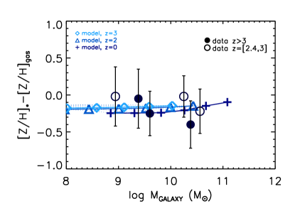
Figure 4: Difference in metallicity between galactic components and its evolution as a function of the stellar mass. Models as in Fig. 3. Crosses, triangles and diamonds give the position on each track at $z=0$, $z=2$ and $z=3$, respectively. Single galaxy measurements in the redshift bins [2.4-3[ (empty circles) and [3,3.7] (full circles), respectively, as compiled by Sommariva et al. (2012) are also shown.

4.3 The mass- average stellar metallicity relation

We note that since the average metallicity in gas increases with galactic mass, we expect L13 model to predict also a stellar-mass metallicity relation. We show that it is broadly consistent with observations in Fig. 5, where we plot the evolution in the stellar metallicity as a function of the stellar mass. Crosses, triangles and diamonds give the position on each track at $z=0$, $z=2$ and $z=3$, respectively. We also show the fit to the local observed relation (Panter et al., 2008, thick maroon line) and single galaxy measurements in the redshift bins [2.4-3[ (empty circles) and [3,3.7] (full circles), respectively, as compiled by Sommariva et al. (2012).

From the model-to-data comparison point of view, we highlight that, at $z\sim 0$, the predictions for high mass galaxies seem to match the observations, whereas there is some tension at the low mass end. On the theoretical side, the slope can be further steepened by acting on the relation between $\nu$ and the initial mass. The normalization of the predicted relation can be further adjusted by acting on the yield and of $z_{F}$. These where however chosen to match the both the $z\sim 0$ and $z\sim 2$ mass-metallicity relation of the gas-phase. On the observational side, a caveat is that $z\sim 0$ data include passive galaxies, which tend to be the most massive and metal rich galaxies. We can therefore expect a milder observational slope in the mass-stellar metallicity relation when selecting only star forming galaxies, in better agreement with our model. The existence of metallicity gradients and aperture effects may further complicate the comparison between data and models. On the other hand, while we predict mass-weighted metallicities, the observables in questions are luminosity-weighted quantities. The difference between luminosity-weighted and mass-weighted metallicity is negligible in massive, old, non-star forming galaxies (e.g. Arimoto & Yoshii, 1987), which make the high mass end of the local relation in Fig. 5. At smaller masses, the mass-averaged Z are slightly larger than the luminosity-averaged ones, since the latter give more weight to the earliest low-metallicity stellar populations (see e.g. Pipino et al., 2006). This may explain the offset between z=0 predictions and observations at the low-mass end in Fig.5.

In our models we do see an evolution in the metallicity with redshift at a given mass at $z<2$. This is slightly ($\sim 0.1$dex) smaller to that predicted in the gas phase, and shown in L13 (their Fig. 7). No apparent evolution is predicted between $z=2$ and $z=3$. L13 model, however, predicts an evolution of the metallicity in this range, and the variation can be readily estimate as follows: when the nebular emission line correction is included $sSFR(z\geq 3)\sim 6$/Gyr , whereas $sSFR(z=2)\sim 2$/Gyr (e.g. Stark et al., 2013). If we apply Eq. 16, we would infer an increase in metallicity by a factor of $\sim 2$ (0.3 dex) between redshift $z\sim 3$ and $z\geq 2$ matching the observational data (e.g. Maiolino et al., 2008). In the same time-frame, however, given these $sSFR$, galaxies increase their mass by at least a factor of 2, therefore they move almost diagonally in the $logZ_{gas}-logM_{GALAXY}$ plane. Since in these earlier phases the average stellar metallicity tracks very well the gas metallicity, the model predicts a similar evolution also in the $logZ_{*}-logM_{GALAXY}$ plane. The combination of the two effects lead to an apparent non evolution in the mass-metallicity plane, as galaxies move along a given track close to the 1:1 relation. They will then move up in metallicity at almost constant mass at $z<2$, when the sSFR is such that the stellar mass increase is milder than the change in $Z$.

Sommariva et al. (2012), on the basis of the same data displayed in Fig. 5 seem to favor instead a lack of evolution at all redshifts. It is however important to note the large observational errors and the scatter affecting the $z>2$ measurements of a few single galaxies.

For comparison, we display the evolution of a galaxy evolving as a closed box model (solid black line) in Fig. 5. We can safely conclude that the data strongly disfavor closed box and favor flow-through models like that of L13.

It also useful to remind the danger of comparing mass-weighted predicted quantities to luminosity-weighted observables. This effect is more important at high z, when galaxies feature high SFRs. We stress again that the $z\sim 0$ data mix active and passive galaxies, whereas the high redshift data-points refer to star-forming galaxies. Moreover, while $z\sim 0$ metallicities are mostly related to the optical part of the spectrum, in high redshift galaxies are derived by means of UV absorption lines (Rix et al., 2004). Therefore a direct and robust, entirely empirical, comparison between the metallicity of the bulk of the stars in galaxies at different redshift has yet to come.

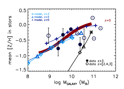
Figure 5: Stellar metallicity evolution as a function of the stellar mass. Models as in Figs. 3 and 4. Crosses, triangles and diamonds give the position on each track at $z=0$, $z=2$ and $z=3$, respectively. The predictions for the Closed Box Model system with $\nu=0.3$/Gyr are shown by the (almost vertical) solid black line. The fit to the local observed relation (Panter et al., 2008, thick solid line) and single galaxy measurements in the redshift bins [2.4-3[ (empty circles) and [3,3.7] (full circles), respectively, as compiled by Sommariva et al. (2012) are also shown.

5 Discussion and Conclusions

5.1 The gas phase metallicity

5.1.1 On the variation of the $Z$ as a function of the sSFR evolution

In this paper we explored the dependence of gas-phase metallicity on the specific star formation rate. In particular, we derived general analytic formulae that relate the gas phase metallicity to both the infall-to-star formation rate ratio and the sSFR, for the case of single-zone single-phase galaxies and a linear Schmidt (1959) star formation law. The derived relations take the typical form $Z(sSFR)={y_{Z}\over\Lambda(sSFR/\nu)}+I(sSFR/\nu)$, where $I$ is the integral of the past enrichment history over the sSFR.

In this article, both the inflow- and the outflow-to-star formation rate ratios are functions of time (equivalently of the sSFR) and may depend on the input cosmology, the amount of gas that may penetrate the star forming regions of galaxies, and the adopted star formation law. It is important to stress that this approach is different from that adopted in many analytical chemical evolution works in the literature, and still in use to interpret the metallicity of galaxies. These studies adopt $\Lambda$ and $\eta$ constant, that is they do not take into account that realistic outflow- and inflow-to-star formation rate ratios may change with time as the result of the evolution of the galaxy. Therefore, when they are compared to data at a given redshift, they can only give a simple parameterized understanding of the mass-metallicity relation at that fixed epoch, rather than offering a comprehensive view of galaxy evolution with time.

We show that in many circumstances (early evolution, quasi-steady state evolution with slowly decreasing sSFR) a good estimate of the gas-metallicity is obtained by the value $Z_{L13}^{id}$ that the system would have if in steady-state evolution with the infall-to-star formation ratio set by the current value of the sSFR (Eq. 11), that is as in the ideal regulator case of L13. On the other hand, a metallicity obtained by current value of the infall-to-star formation rate, i.e. $Z_{L13}$(Eq. 8, L13 non ideal regulator case), would slightly overestimate the current metallicity of the system. These two values bracket with high accuracy the current metallicity of the system. Therefore, we provide the formal justification to L13 approximations and extend their validity to a larger range of cases. In particular, the formula adopted by L13 for the ideal case is exact for systems with $\Lambda-\eta>1$ and $\Lambda,\eta=const$. It is also a good approximation of the actual metallicity for galaxies with slowly decreasing accretion rates.

Also, we add that, since we did not specify anything on both the size and the geometry of what we called the “galaxy”, the equations in principle hold at both the local (i.e. for each star forming region) and the global galaxy level, with the latter being a suitable weighted average of the single star forming regions. Such a theoretical expectation seems to be corroborated by very recent observations (Rosales-Ortega et al., 2012).

Finally, L13 (their Fig. 7) show the predictions for the mass-metallicity relation at $z>0$ in some specific cases calibrated on either the Mannucci et al. (2010) or the Tremonti et al. (2004) $z\sim 0$ relations. A qualitative agreement with the $z\sim 2$ data is achieved. In this paper we do not repeat the exercise. However, in Fig. 6, we plot the $z<4$ tracks of the models shown in Fig. 5, compared to the full three-dimensional fundamental metallicity relation as given by Mannucci et al. (2010, their Eq. 2). In the L13 framework, galaxies evolve along the surface given by the fundamental metallicity relation.

Also, we wish to highlight the following point, which was not discussed in L13, but it is implied by the assumed $Z=f(sSFR)$ relation at a fixed epoch. It is in fact relevant to the data-model comparison to note that the galaxies in the $z=2$ and $z=3$ observational samples show a rather flat SFR-mass relation (c.f. Mannucci et al., 2009, their Fig. 6), by virtue of their selection. This relation is flatter than the typical SFR-mass relation for star forming galaxies at the same epoch (e.g. Daddi et al., 2007). If we assume that the observational samples are culled out from the star forming population at their respective redshifts, the selection of the most massive galaxies with systematically below the average SFR creates a bias such that the most massive galaxies tend to systematically have the lowest sSFR, and thus to be the most metal rich at their mass scale (at least this is the expectation in the L13 theoretical framework). By virtue of the SFR selection threshold, the low mass galaxies will have higher than average SFR, and hence a lower metallicity than the typical star forming galaxy at the same redshift and mass. This means that the observational samples might be biased in the direction of having a steeper mass-metallicity relation than the typical relation of an unbiased sample of star forming galaxies at the same redshift. Therefore any empirical conclusion on the evolution in the slope of the mass-metallicity relation must be treated with caution.

5.1.2 On the L13 metallicity formula: accuracy and comparison to full numerical chemical evolution models

In order to quantify the accuracy of the L13 approximations, we compared them to a full and direct numerical integration of the same equations, finding an excellent agreement ($<0.1$ dex) for three orders of magnitude in the sSFR and almost 2 dex in $Z$.

By comparing tracks in the $Z-sSFR$ plane given by either the L13 approximation or the Closed Box relation to the predictions of full numerical chemical evolution models which relax some of the simplifying assumptions adopted in the analytic case, we find that star forming $z<2$ (spiral) galaxies, where the sSFR slowly decreases with time, the system evolves along the locus of the steady-state solutions of decreasing gas fraction and increasing metallicity, exactly as in the L13 gas-regulated model. In particular, these system seeks the steady state metallicity without attaining it and the current metallicity is set by the current value of the sSFR.

Fast-forming (elliptical) galaxies, evolve at higher sSFR than slowly-evolving systems at the same metallicity, with a remarkable similarity to the well-known behavior in the [$\alpha$/Fe]-mass plane. Their track in the sSFR-Z plane is better approximated by Closed Box models.

5.1.3 The SFR as the second parameter in L13 and other special cases (closed box, evolution at constant gas mass)

The actual functional form of a mass-(s)SFR-metallicity relation is quite controversial, with empirical findings also including claims of a reversal (namely high SFR would correspond to high metallicity) at high stellar masses (e.g. Yates et al., 2012) and a lack of any SFR effects at all masses (e.g. Sanchez et al., 2013). Clearly, differences may originate from a variety of empirical issues related to the sample specifics (including redshift range and aperture effects, e.g. Sanchez et al., 2013) as well as to the methods used to derive the metallicity (and the SFR).

In L13 the metallicity dependes inversely on the sSFR. To some extent we expect a smaller dependence on the sSFR as a second parameter at high masses, simply because in L13 $\nu$ becomes larger and hence the term $sSFR/\nu$ smaller than the other terms in the denominator of Eq. (8). In other words, the most massive models settle earlier on an evolutionary track where the metallicity quickly asymptotes to the yield, and the second parameter effect caused by variations in the (s)SFR become consequently small. It seems more difficult to explain a reversal of the trend above a given stellar mass scale.

Moreover, L13 model is meant to reproduce the average galaxy, therefore, it does not take into account that episodic bursts and mergers may also happen and move galaxies further out of the “average” quasi steady-state evolution represented by our tracks.

As a matter of fact, in this paper we also show that an anti-correlation between $Z$ and sSFR is found also in the early evolutionary phases of the Closed Box model.

In other works (e.g. Davé et al., 2012), the case $\Lambda-\eta=1$ (which is a generalization of Larson 1972’s extreme infall in the context of analytic chemical evolution) has been dubbed “steady-state”. In other words, all the net accreted gas is used up to form stars. More specifically, it is the $\Lambda=1,\eta=0$ case which is known as the “extreme infall”. It has the property of preserving the gas mass, rather than the gas fraction, and that the metallicity would evolve as $Z=(Z_{A}+y_{z})\,(1-exp(1/\mu-1))$, asymptotically approaching the yield for $\mu$ approaching 0.

The generalization of extreme infall where both inflows and outflows are present ($\Lambda$, $\eta=\,const$), has the following analytical solution for the metallicity:

$$Z={(Z_{A}\Lambda+y_{z})\over\Lambda}\biggl{\{}1-e^{-\Lambda\,(1/\mu-1)}\biggr{\}}$$ (45)

or equivalently:

$$Z={[Z_{A}(1+\eta)+y_{z}]\over(1+\eta)}\biggl{\{}1-e^{-(1+\eta)\,(1/\mu-1)}\biggr{\}}$$ (46)

It is important to note here that, despite assuming the validity of the condition $\Lambda-\eta\simeq 1$, Davé et al. (2012) do not fully derive these solutions. In fact, they base their model on their Eq. 9. We find that their formula can be re-arranged, after discarding the trivial solution $Z(t)=0$ and assuming that $Z\neq Z_{A}$, as: $Z\sim{[Z_{A}(1+\eta)+y_{z}]\over(1+\eta)}$, which is only an approximation to our exact solutions (e.g., Eq. 46), valid when the gas fraction is small (as pointed out also by Dayal et al., 2013). This latter condition ($\mu<<1$) is unlikely to be true in high redshift galaxies.

When the galaxy is in its asymptotic regime at constant gas mass, that is $Z\simeq Z_{A}+y_{z}$, the only way to increase its metallicity is by acting on $Z_{A}\neq 0$. In the first place, in the light of our full analytic derivation, we stress that the correct solutions for $Z$ in a standard analytic chemical evolution model when the infalling gas metallicity changes with time and it is linked to the past history of the galaxy, must take into account that $Z_{A}=Z_{A}(t)$ in the formal integration (Eq. 22 in this paper, see also the implementation of galactic fountains in Recchi et al., 2008).

We then note that when $Z_{A}$ drives the metallicity, it increases with time in a manner that is not necessarily linked to the sSFR evolution. In other words, in systems with $\Lambda(-\eta)\sim 1$ the gas fraction still changes with time, leading to changes in the sSFR which are un-correlated to variations in the gas metallicity (in principle set by yield, and varied through a changing metallicity in the “re-accretion” of previously ejected material). This also implies that the scatter around the average $Z-sSFR$ relation cannot be described by the same equation that governs the $Z=Z(sSFR)$ evolution as in L13. On the contrary, in Davé et al. (2012), the explanation of the scatter (and of the $Z-sSFR$ anti-correlation) requires stochastic events that drive the galaxies out of equilibrium, either enhancing the SFR (e.g. mergers) or momentarily suppressing it (e.g. a sudden decrease in the accretion), and causing either a decrease or a increase in $Z$, respectively. This perspective is not dissimilar to the explanation given by Mannucci et al. (2010) when they first presented the empirical results on the “fundamental metallicity relation”, and it is further extended in other recent work (e.g. Forbes et al., 2013) which depict both the mass-SFR and the mass-Z relations as the result of statistical equilibrium in the galaxy population at a given epoch.

5.2 Stellar metallicities in the L13 model

As a further extension of the L13 model, we show that it also naturally predicts a mass-metallicity relation in the stellar component which matches the current data at different epochs.

We compare our predictions to the data, and despite the encouraging qualitative agreement, no firm quantitative conclusions can be drawn due to: i) the large scatter in the high redshift data; ii) the lack of consistency among the stellar metallicity measurements at different epochs; and iii) the presence of both passive and star forming galaxies in the $z\sim 0$ dataset.

L13’s slowly evolving galaxies therefore match both the observed cosmic evolution in the gas and in the average stellar metallicity at a given mass. This is a consequence of the fact that the average stellar metallicity systematically lags $\sim 0.1-0.2$ behind the gas metallicity of the same galaxy (as observed).

In evolved ($\mu<<1$) systems, such a small difference can be explained by the fact the both the gas and the average stellar metallicity tends to the yield. Whereas, during earlier stages of the evolution, the explanation lies in the fact that the SFR is steadily increasing in time. Therefore the youngest stellar generations (whose composition is the same of the gas-phase) have a larger weight in the computation of the average stellar metallicity.

These findings imply that the evolution of the average stellar metallicity in the early phases of L13 galaxies as a function of the sSFR can be approximated by the same formula adopted for the gas phase metallicity.

Appendix

The impact of the assumed star formation law.

Let us discuss the impact of a more general star formation law on our results, that, for the purpose of this discussion, we write as $\psi=\nu M_{gas}^{(1+x)}$. In this paper we presented the results for the case $x=0$. Such a linear Schmidt volumetric relation is a standard assumption in the literature and it has the advantage of a slight simplification of the calcultions presented in this paper. To corroborate our assumption, we note that in a recent paper, Krumholz et al. (2012) showed that a simple volumetric star formation law as the one adopted in our paper, can explain a wide range of both local and high-redshift observations.

Furthermore, it leads to a relation with exponent $1.5$ if the star formation efficiency is expressed in units of the local free fall time, and this latter quantity is in turn expressed as a function of the gas volume density. This also ensures compatibility with the expression adopted in studies where SFR and density are in units of surface which assume an exponent $x\sim 1.4$.

It is well known that the solutions of the form $Z=Z(\mu)$ of analytical chemical evolution models do not explictly depend on the SFR (and its law). Therefore, the particular star formation law adopted does not influence these general results. It is the conversion of the gas fraction into sSFR that introduces a dependence on the assumed star formation law in the equations of the form $Z=Z(sSFR)$. To see the impact of the change let us proceed as in the main body of the paper, namely let us focus on the steady-state solutions and the derive more general statements.

In the case of the steady state, the results presented in Eqs. 12, 13, 14 and 16 (its first row), as well as other results like Eqs. 32 and 33, will not depend on $x$ as they do not feature any explicit dependence on the star formation law.

On the other hand, when $x\neq 0$, Eq. 1 would be

$$sSFR/\nu\propto{\mu\over 1+\mu}\mu^{x}$$

(e.g. Reddy et al. (2006), when x=0.4), and Eq. 15 would read as

$$sSFR/\nu=(\Lambda-\eta-1)M_{gas}^{x}\,.$$

The steady state solution presented in Sec. 3.2 (Eq. 16 second row) will then be

$$Z={1\over 1+\eta+sSFR/(\nu M_{gas}^{x})}\,,$$

where for simplicity we ignore the metallicity of the infalling gas. If $x>0$, the system behaves as if it has a higher effective star formation efficiency $\nu M_{gas}^{x}$. Moreover $x\neq 0$ would imply an evolution at constant gas fraction and metallicity with the sSFR still changing in time as $M_{gas}^{x}$.

Given the close link between $I_{1}$ (Eq.11), Eq. 24 and the steady-state solution (Eq. 16), we expect a similar variation, namely the apperarence of a factor $\sim M_{gas}^{x}$ in the expression for $Z_{L13}$ in both the ideal and non indeal case, as well as in the general solutions. More quantitatively, this happens because the term $G$ in the differential equation 19 will now be:

$$G(sSFR)={1+{Z_{A}\Lambda\over y_{z}}\over sSFR/\nu((1+x)(\Lambda-\eta-1)M_{gas}^{x}-sSFR/\nu)}\,,$$ (47)

leading to a change in the expression for $F(sSFR)$ too. The qualitative description of the galaxy behavior will not change: as these models tend to a $\Lambda\sim 1$ (constant gas mass) evolution in the long term, the factor $M_{gas}^{x}$ will be merely a constant for all practical purposes.

References

- [] Belli, Sirio; Jones, Tucker; Ellis, Richard S.; Richard, Johan 2013, ApJ, 772, 141
- [] Bordoloi, R., et al., 2011, ApJ, 743, 10
- [] Bordoloi, R., et al., 2013, ApJ, submitted, arXiv:1307.6553B
- [] Bouché N., et al., 2010, ApJ, 718, 1001
- [] Calura, F.; Pipino, A.; Chiappini, C.; Matteucci, F.; Maiolino, R. 2009, A&A, 504, 373
- [] Cicone, C., et al., 2013, A&A accepted, arXiv:1311.2595
- [] Cid Fernandes R., Asari N. V., Sodré L., Stasińska G., Mateus A., Torres-Papaqui J. P., Schoenell W., 2007, MNRAS, 375, L16
- [] Clayton D. D., 1988, MNRAS, 234, 1
- [] Cresci G. et al. 2011, arXiv1110.4408
- [] Christensen, L., et al., 2012, MNRAS, 427, 1953
- [] Cullen, F., Cirasuolo, M., McLure, R.J., Dunlop, J.S., 2013, arXiv:1310.0816
- [] Daddi E., et al., 2007, ApJ, 670, 156
- [] Dalcanton J. J., 2007, ApJ, 658, 941
- [] Davé, Romeel; Finlator, Kristian; Oppenheimer, Benjamin D. 2012, MNRAS, 421, 98
- [] Dayal, P., Ferrara, A., Dunlop, J.S., 2013, MNRAS, 430, 2891
- [] Dutton A. A., van den Bosch F. C., Dekel A., 2010, MNRAS, 405, 1690
- [] Edmunds M. G., 1990, MNRAS, 246, 678
- [] Ellison, S.L., Patton, D.R., Simard, L., McConnachie, A.W., 2008, ApJL, 672, L107
- [] Elbaz D., et al., 2007, A&A, 468, 33
- [] Erb D. K., Steidel C. C., Shapley A. E., Pettini M., Reddy N. A., Adelberger K. L., 2006, ApJ, 646, 107
- [] Erb D. K., Shapley A. E., Pettini M., Steidel C. C., Reddy N. A., Adelberger K. L., 2006, ApJ, 644, 813
- [] Forbes, J.C., Krumholz, M.R., Burkert, A., Dekel, A., arXiv:1311.1509
- [] Gallazzi, Anna; Charlot, St phane; Brinchmann, Jarle; White, Simon D. M. 2006, MNRAS, 370, 1106
- [] Garnett D. R., 2002, ApJ, 581, 1019
- [] González V., Labbé I., Bouwens R. J., Illingworth G., Franx M., Kriek M., Brammer G. B., 2010, ApJ, 713, 115
- [] Halliday, C., et al., 2008, A&A, 479, 417
- [] Hartwick, F. D. A. 1976, ApJ, 209, 418
- [] Henry, A., et al., 2013, arXiv:1309.4458
- [] Köppen J., Edmunds M. G., 1999, MNRAS, 306, 317
- [] Köppen J., Weidner C., Kroupa P., 2007, MNRAS, 375, 673
- [] Lara-López M. A., et al., 2010, A&A, 521, L53
- [] Lara-López M. A., et al., 2013, MNRAS, 434, 451
- [] Larson, R.B. 1972, Natur, 236, 21
- [] Leja, J., et al., 2013, ApJL, 778, 24
- [] Lequeux, J.; Peimbert, M.; Rayo, J. F.; Serrano, A.; Torres-Peimbert, S. 1979, A&A, 80, 155
- [] Lilly, S.J., Carollo, C.M., Pipino, A., Renzini, A., Peng, Y., 2013, ApJ, 772, 19
- [] Maier C., Lilly S. J., Carollo C. M., Stockton A., Brodwin M., 2005, ApJ, 634, 849
- [] Maier C., Lilly S. J., Carollo C. M., Meisenheimer K., Hippelein H., Stockton A., 2006, ApJ, 639, 858
- [] Maiolino R., et al., 2008, A&A, 488, 463
- [] Mannucci F., et al., 2009, MNRAS, 398, 1915
- [] Mannucci F., Cresci G., Maiolino R., Marconi A., Gnerucci A., 2010, MNRAS, 408, 2115
- [] Mannucci, F.; Salvaterra, R.; Campisi, M. A. 2011, MNRAS, 414, 1263
- [] Matteucci F., 1994, A&A, 288, 57
- [] Matteucci F., 2001, The chemical evolution of the Galaxy, Astrophysics and space science library, Volume 253, Dordrecht: Kluwer Academic Publishers
- [] Matteucci, F., Brocato, E., 1990, ApJ, 365, 539
- [] Matteucci, F., Chiosi, C., 1983, A&A, 123, 121
- [] Moster, Benjamin P.; Somerville, Rachel S.; Maulbetsch, Christian; van den Bosch, Frank C.; Macci , Andrea V.; Naab, Thorsten; Oser, Ludwig 2010, ApJ, 710, 903
- [] Nakajima, K., Ouchi, M., 2013, arXiv:1309.0207
- [] Neistein E., Dekel A., 2008, MNRAS, 383, 615
- [] Newman, S.F., et al., 2012, ApJ, 761, 43
- [] Niino, Y., 2012, ApJ, 761, 126
- [] Noeske K. G., et al., 2007, ApJ, 660, L43
- [] O’Connell, R.W., 1976, ApJ, 206, 370
- [] Oliver S., et al., 2010, MNRAS, 405, 2279
- [] Pagel B. E. J., Patchett B. E., 1975, MNRAS, 172, 13
- [] Pannella M., et al., 2009, ApJ, 698, L116
- [] Panter B., Jimenez R., Heavens A. F., Charlot S., 2008, MNRAS, 391, 1117
- [] Peeples, Molly S.; Shankar, Francesco 2011, MNRAS, 417, 2962
- [] Peng, Y-J et al. 2010, ApJ, 721, 193
- [] Pipino, A., Calura, F., Matteucci, F., 2013, MNRAS, 432, 2541
- [] Pipino A., Devriendt J. E. G., Thomas D., Silk J., Kaviraj S., 2009, A&A, 505, 1075
- [] Pipino, A.; Fan, X. L.; Matteucci, F.; Calura, F.; Silva, L.; Granato, G.; Maiolino, R. 2011, A&A, 525, 61
- [] Pipino A., Matteucci F., 2004, MNRAS, 347, 968
- [] Pipino A., Matteucci F., Chiappini, C., 2006, ApJ, 638, 739
- [] Richard, Johan; Jones, Tucker; Ellis, Richard; Stark, Daniel P.; Livermore, Rachael; Swinbank, Mark 2011, MNRAS, 413, 643
- [] Recchi S., Spitoni E., Matteucci F., Lanfranchi G. A., 2008, A&A, 489, 555
- [] Reddy, Naveen A.; Steidel, Charles C.; Fadda, Dario; Yan, Lin; Pettini, Max; Shapley, Alice E.; Erb, Dawn K.; Adelberger, Kurt L. 2006, ApJ, 644, 792
- [] Rosales-Ortega, F.F., et al. 2012, ApJ, 756, L31
- [] Sanchez, S.F., et al., 2013, A&A, 554, 58
- [] Sakstein J., Pipino A., Devriendt J. E. G., Maiolino R., 2011, MNRAS, 410, 2203
- [] Savaglio S., et al., 2005, ApJ, 635, 260
- [] Schmidt, M., 1959, ApJ, 129, 243
- [] Schmidt, M., 1963, ApJ, 137, 758
- [] Sommariva, V.; Mannucci, F.; Cresci, G.; Maiolino, R.; Marconi, A.; Nagao, T.; Baroni, A.; Grazian, A. 2012, A&A, 539, 136
- [] Spitoni, E.; Calura, F.; Matteucci, F.; Recchi, S. 2010, A&A, 514, 73
- [] Stark, Daniel P.; Schenker, Matthew A.; Ellis, Richard; Robertson, Brant; McLure, Ross; Dunlop, James 2013, ApJ, 763, 129
- [] Stott, J.P., et al., 2013, MNRAS, 436, 1130
- [] Tinsley B. M., 1980, FCPh, 5, 287
- [] Tremonti C. A., et al., 2004, ApJ, 613, 898
- [] Troncoso, P., et al., 2013, arXiv:1311.4576
- [] Twarog B. A., 1980, ApJ, 242, 242
- [] Yates R. M., Kauffmann G., Guo Q., 2011, arXiv, arXiv:1107.3145
- [] Yuan, T.-T.; Kewley, L. J.; Richard, J. 2013, ApJ, 763, 9
- [] Weiner, B.J., et al., 2005 ApJ, 620, 595
- [] Wuyts, Eva; Rigby, Jane R.; Sharon, Keren; Gladders, Michael D. 2012, ApJ, 755, 73
- [] Zahid, H. J.; Bresolin, F.; Kewley, L. J.; Coil, A. L.; Dav , R. 2012, ApJ, 750, 120
- [] Zahid, H. J. et al., 2013, arXiv:1310.4950