Nature and dynamics of overreflection of Alfv${\rm\acute{e}}$n waves in MHD shear flows

Abstract

Our goal is to gain new insights into the physics of wave overreflection phenomenon in MHD nonuniform/shear flows changing the existing trend/approach of the phenomenon study. The performed analysis allows to separate from each other different physical processes, grasp their interplay and, by this way, construct the basic physics of the overreflection in incompressible MHD flows with linear shear of mean velocity, ${\bf U}_{0}=(Sy,0,0)$, that contain two different types of Alfv${\rm\acute{e}}$n waves. These waves are reduced to pseudo- and shear shear-Alfv${\rm\acute{e}}$n waves when wavenumber along $Z$-axis equals zero (i.e., when $k_{z}=0$). Therefore, for simplicity, we labelled these waves as: P-Alfv${\rm\acute{e}}$n and S-Alfv${\rm\acute{e}}$n waves (P-AWs and S-AWs). We show that: (1) the linear coupling of counter-propagating waves determines the overreflection, (2) counter-propagating P-AWs are coupled with each other, while counter-propagating S-AWs are not coupled with each other, but are asymmetrically coupled with P-AWs; S-AWs do not participate in the linear dynamics of P-AWs, (3) the transient growth of S-AWs is somewhat smaller compared with that of P-AWs, (4) the linear transient processes are highly anisotropic in wave number space, (5) the waves with small streamwise wavenumbers exhibit stronger transient growth and become more balanced, (6) maximal transient growth (and overreflection) of the wave energy occurs in the two-dimensional case – at zero spanwise wavenumber.

To the end, we analyze nonlinear consequences of the described anisotropic linear dynamics – they should lead to an anisotropy of nonlinear cascade processes significantly changing their essence, pointing to a need of revisiting the existing concepts of cascade processes in MHD shear flows.

1 Introduction

Nonuniform flows are ubiquitous both in nature and in laboratory. They occur in atmospheres, oceans, solar wind, stars, astrophysical disks, pipe flows, tokamak reactors, etc. Complex dynamics of these systems is, in many respects, a consequence of their nonuniform kinematics. One of the basic manifestations of flow shear is wave overreflection phenomenon – substantial growth of counter-propagating wave perturbations – that occurs universally whenever flow has non-zero shear. For instance, in astrophysical discs, there is the overreflection of spiral-density waves, in the atmosphere – internal-gravity waves, in the solar wind – MHD waves, etc.

The essence of the overreflection is the following. If initially in a shear flow exist just waves having definitely directed group velocity and, consequently, propagating in one direction (i.e. counter-propagating waves are absent initially), in the course of time, appears and substantially increase counter-propagating waves, i.e., waves that have oppositely (to the initial waves) directed group velocity. Of course, if the initial/incident waves are localized in the flow shear direction, the overreflection phenomenon has visual manifestation – it appears reflected (also localized in the shear direction) waves having larger, then incident waves, amplitude. However, in the non-modal approach, investigating the dynamics of spatial Fourier harmonics of waves (so called, Kelvin waves) that are not localized in the physical space, the visual manifestation is absent and one can mathematically describe the overreflection by the appearance and increase of counter-propagating waves, i.e. – waves having oppositely directed group velocity. We aim to go deeper into the physical mechanism responsible for this overreflection in an incompressible MHD shear flow.

The overreflection phenomenon is usually analysed on the basis of a single second-order ordinary differential (wave) equation (e.g., see seminal papers on overreflection Goldreich & Tremaine, 1978, 1979; Lindzen & Barker, 1985; Farrell & Ioannou, 1993b). This approach describes counter-propagating waves by a single/physical variable and, consequently, possible dynamical processes between these waves (e.g., their coupling) are, in fact, left out of consideration. To fill this gap – to reduce the perturbation equations to the set of first order differential equations for individual counter-propagating wave – we propose, at first, to find “eigen-variable” for each wave component. I.e., to find variables for which the linear matrix operator is diagonal in the shearless limit. Then, one have to generalize the eigen-variables for non-zero shear case. The generalization is not unique possible procedure. But the optimal one is quite easily findable. In the considered MHD flow, the generalized variables are the renormalized Els$\ddot{a}$sser variables (see equations 2.12). Resulting first order ordinary differential equations (written for the generalized variables) separate from each other different physical processes, make it possible to grasp their interplay and understand the basic physics of the overreflection phenomenon. In the renormalized Els$\ddot{a}$sser variables we get two different types of Alfv${\rm\acute{e}}$n waves in incompressible MHD flows with linear shear of mean velocity, ${\bf U}_{0}=(Sy,0,0)$. As it is mentioned in the abstract, these waves are reduced to pseudo- and shear-Alfv${\rm\acute{e}}$n waves when wavenumber along $Z$-axis equals zero (i.e., when $k_{z}=0$). Therefore, for simplicity, we labelled these waves as: P-Alfv${\rm\acute{e}}$n and S-Alfv${\rm\acute{e}}$n waves (P-AWs and S-AWs). We carried out analytical (Kelvin mode) and numerical analysis of the linear dynamics of P-AWs and S-AWs. Our analysis has clearly demonstrated linear coupling between these waves. We describe in detail transient growth of counter-propagating components of P-AWs and S-AWs when only one of them exists initially in the flow. The amplification of these (so-called, transmitted and reflected) waves, i.e. the wave overreflection phenomenon, is determined by the linear coupling of the waves induced by shear flow non-normality.

Historically, the non-normality of shear flows considerably delayed the full understanding of their behavior. In fact, this feature and its dynamical consequences only became well understood by the hydrodynamic community in the 1990s (e.g., see Reddy & Henningson, 1993; Trefethen et al., 1993; Schmid, 2007). Shortcomings of the traditional modal analysis (i.e., spectral expansion of perturbations in time and then analysis of eigenfunctions) for shear flows have been revealed and an alternative Kelvin wave approach – a special kind of the non-modal approach – has become well established and has been extensively used since the 1990s. Kelvin waves represent the basic “elements” of dynamical processes at constant shear rate (Chagelishvili et al., 1996; Yoshida, 2005) and greatly help to understand finite-time transient phenomena in shear flows. In particular, it reveals a channel of linear coupling among different branches/modes of perturbations in shear flows (Chagelishvili et al., 1997b, a), leading to energy exchange between vortex and wave modes and between different wave branches.

A new, bypass transition, concept was also formulated by the the hydrodynamic community to explain the onset of turbulence in spectrally stable shear flows (e.g., see Baggett et al., 1995; Grossmann, 2000; Eckhardt et al., 2007, and references therein) on the basis of the interplay between linear transient growth and nonlinear positive feedback. The bypass scenario differs fundamentally from the classical turbulence scenario, which is based on exponentially growing perturbations in a system that supplies turbulent energy. In the classical case, the nonlinearity is not vital to the existence of the perturbations. Instead, it merely determines their scales, via the direct/inverse cascade.

This breakthrough led to renewed comprehension of different aspects of shear flow dynamics. This paper, being along these lines, aims to provide new insight into the physics of wave overreflection on the example of P-AWs and S-AWs in incompressible MHD flows with linear shear of mean velocity profile. Actually, our study can be of wide applicability:
(i) the method of characterizing overreflection presented here is optimal, moreover, canonical, and can be easily applied for deeper understanding of the overreflection phenomenon in other important cases, such as spiral-density waves in astrophysical discs and internal-gravity waves in stably stratified atmospheres;
(ii) the presented overreflection fits in naturally within the above-mentioned bypass concept. This allows us to adopt schemes and ideas of the bypass concept for the understanding of driven turbulence in MHD shear flows.

The paper is organized as follows. Section 2 is devoted to deriving four first order differential equations (for individual counter-propagating wave) and qualitative analysis of the equations. Section 3 – to the numerical analysis in two and three dimensions. Summary and discussion are given in Section 4 where we also analyze nonlinear consequences of the described linear dynamics and application of the proposed approach to more complex shear flow systems.

2 Physical model and equations

Consider a 3D ideal, incompressible MHD fluid flow with constant/linear shear of velocity, ${\bf U}_{0}=(Sy,0,0)$, and uniform magnetic field, ${\bf B}_{0}=(B_{0},0,0)$, directed along the flow. The linearized dynamical equations for small perturbations to the flow are:

$$\left({{\partial}\over{\partial t}}+Sy{{\partial}\over{\partial x}}\right)v_{x}+Sv_{y}=-{1\over\rho}{{\partial p}\over{\partial x}}~{},~{}~{}~{}~{}~{}~{}~{}~{}~{}~{}~{}~{}~{}~{}~{}~{}~{}~{}~{}~{}~{}$$ (1)

$$\left({{\partial}\over{\partial t}}+Sy{{\partial}\over{\partial x}}\right)v_{y}=-{1\over\rho}{{\partial p}\over{\partial y}}+{B_{0}\over 4\pi\rho}\left({{\partial b_{y}}\over{\partial x}}-{{\partial b_{x}}\over{\partial y}}\right)~{},~{}$$ (2)

$$\left({{\partial}\over{\partial t}}+Sy{{\partial}\over{\partial x}}\right)v_{z}=-{1\over\rho}{{\partial p}\over{\partial z}}+{B_{0}\over 4\pi\rho}\left({{\partial b_{z}}\over{\partial x}}-{{\partial b_{x}}\over{\partial z}}\right)~{},~{}$$ (3)

$${{\partial v_{x}}\over{\partial x}}+{{\partial v_{y}}\over{\partial y}}+{{\partial v_{z}}\over{\partial z}}=0~{},~{}~{}~{}~{}{{\partial b_{x}}\over{\partial x}}+{{\partial b_{y}}\over{\partial y}}+{{\partial b_{z}}\over{\partial z}}=0~{},$$ (4)

$$\left({{\partial}\over{\partial t}}+Sy{{\partial}\over{\partial x}}\right)b_{y}=B_{0}{{\partial v_{y}}\over{\partial x}}~{},~{}~{}~{}~{}~{}~{}~{}~{}~{}~{}~{}~{}~{}~{}~{}~{}~{}~{}~{}~{}~{}~{}~{}~{}~{}~{}~{}~{}~{}$$ (5)

$$\left({{\partial}\over{\partial t}}+Sy{{\partial}\over{\partial x}}\right)b_{z}=B_{0}{{\partial v_{z}}\over{\partial x}}~{},~{}~{}~{}~{}~{}~{}~{}~{}~{}~{}~{}~{}~{}~{}~{}~{}~{}~{}~{}~{}~{}~{}~{}~{}~{}~{}~{}~{}~{}$$ (6)

where: $\rho$ is the unperturbed density; $~{}p,$ $\bf v$ and $\bf b$ are the pressure, velocity and magnetic field perturbations, respectively.

The dynamic equations permit the decomposition of perturbed quantities into Kelvin waves, or spatial Fourier harmonics (SFHs):

$$\Psi(x,y,z,t)=\tilde{\Psi}(k_{x},k_{y}(t),k_{z},t)\exp(ik_{x}x+ik_{y}(t)y+ik_{z}z)~{},$$ (7)

where $~{}\Psi=\{p,{\bf v},{\bf b}\},$ $~{}\tilde{\Psi}=\{\tilde{p},{\bf\tilde{v}},{\bf\tilde{b}}\}~{}$ and $~{}k_{y}(t)=k_{y0}-Sk_{x}t.$

Introducing the following non-dimensional variables and parameters by taking: $~{}1/S$ as the scale of time; Alfv${\rm\acute{e}}$n velocity, $~{}V_{A}=B_{0}/(4\pi\rho)^{1/2}$, as the scale of velocity perturbation; $~{}B_{0}$ as the scale of magnetic field perturbation,

$$\tau=St~{},~{}~{}~{}k_{y}(\tau)=k_{y}(0)-k_{x}\tau~{},~{}~{}~{}\hat{v}_{y}=\tilde{v}_{y}/V_{A}~{},~{}~{}~{}$$

$$\hat{v}_{z}=\tilde{v}_{z}/V_{A}~{},~{}~{}~{}\hat{b}_{y}=\tilde{b}_{y}/B_{0}~{},~{}~{}~{}\hat{b}_{z}=\tilde{b}_{z}/B_{0}~{},$$ (8)

the above system of equations reduces to the following first order dynamic equations:

$${d\hat{v}_{y}\over d\tau}=2\chi_{p}(\tau)\hat{v}_{y}+i\Omega_{A}\hat{b}_{y}~{},~{}~{}~{}~{}~{}~{}~{}{d\hat{b}_{y}\over d\tau}=i\Omega_{A}\hat{v}_{y}~{},~{}~{}~{}~{}~{}~{}~{}~{}~{}$$ (9)

$${d\hat{v}_{z}\over d\tau}=2\chi_{s}(\tau)\hat{v}_{y}+i\Omega_{A}\hat{b}_{z}~{},~{}~{}~{}~{}~{}~{}~{}{d\hat{b}_{z}\over d\tau}=i\Omega_{A}\hat{v}_{z}~{},~{}~{}~{}~{}~{}~{}~{}$$ (10)

where

$$\chi_{p}(\tau)={k_{x}k_{y}(\tau)\over k^{2}(\tau)}~{},~{}~{}~{}\chi_{s}(\tau)={k_{x}k_{z}\over k^{2}(\tau)}~{},~{}~{}~{}$$

$$k^{2}(\tau)\equiv k_{x}^{2}+k_{y}^{2}(\tau)+k_{z}^{2}~{},~{}~{}~{}\Omega_{A}\equiv{k_{x}V_{A}\over S}~{}.~{}~{}~{}$$ (11)

$\Omega_{A}$ is non-dimensional Alfv${\rm\acute{e}}$n wave frequency.

One can say, that $~{}\hat{v}_{y}$, $~{}\hat{v}_{z}$, $\hat{b}_{y}~{}$ and $~{}\hat{b}_{z}~{}$ are physical variables, but not eigen ones for the counter-propagating P-AWs and S-AWs. Here we start our optimal route to the description of the overreflection phenomenon the essence of which is outlined in the introduction: initially, one have to define eigen variable for each wave components in the shearless limit (for which the linear matrix operator is diagonal). Then, one have to generalize the eigen variables for non-zero shear case and rewrite the dynamic equations for them. Fortunately, in the considered MHD flow, one can use the Els$\ddot{a}$sser variables as the generalized ones,

$$Z_{p}^{\pm}=\hat{v}_{y}\mp\hat{b}_{y}~{},~{}~{}~{}Z_{s}^{\pm}=\hat{v}_{z}\mp\hat{b}_{z}~{}.~{}~{}~{}$$ (12)

Inserting the Els$\ddot{a}$sser variables into equations (2.9) and(2.10), one get the set of the four, first order differential equations describing the dynamics of P-Alfv${\rm\acute{e}}$n (labelled by the index “p”) and S-Alfv${\rm\acute{e}}$n (labelled by the index “s”) wave SFHs:

$${dZ_{p}^{+}\over d\tau}=-i\Omega_{A}Z_{p}^{+}+\chi_{p}(\tau)Z_{p}^{+}+\chi_{p}(\tau)Z_{p}^{-}~{},~{}~{}~{}$$ (13)

$${dZ_{p}^{-}\over d\tau}=i\Omega_{A}Z_{p}^{-}+\chi_{p}(\tau)Z_{p}^{-}+\chi_{p}(\tau)Z_{p}^{+}~{},~{}~{}~{}~{}~{}$$ (14)

$${dZ_{s}^{+}\over d\tau}=-i\Omega_{A}Z_{s}^{+}+\chi_{s}(\tau)Z_{p}^{+}+\chi_{s}(\tau)Z_{p}^{-}~{},~{}~{}~{}$$ (15)

$${dZ_{s}^{-}\over d\tau}=i\Omega_{A}Z_{s}^{-}+\chi_{s}(\tau)Z_{p}^{-}+\chi_{s}(\tau)Z_{p}^{+}~{}.~{}~{}~{}~{}~{}$$ (16)

One can see that the linear matrix operator of the equations (written for the eigen variables) is not diagonal in shear flow. I.e. the dynamics of the waves are not separated to each other any more.

2.1 Spectral energy

Strictly speaking, the energy of waves should be determined in the framework of nonlinear problems. However, usually, the concept of energy is introduced in solving linearized problems (Stepanyants & Fabrikant, 1989). We also do the same to get a feeling of the dynamics of quadratic forms of physical variables.

The energy of an individual SFH (total spectral energy) is the sum of kinetic and magnetic ones:

$$E(k_{x},k_{y}(\tau),\tau)={\rho V_{A}^{2}\over 2}\left(|\hat{v}_{x}|^{2}+|\hat{v}_{y}|^{2}+|\hat{v}_{z}|^{2}+|\hat{b}_{x}|^{2}+|\hat{b}_{y}|^{2}+|\hat{b}_{z}|^{2}\right)=~{}~{}~{}~{}~{}~{}~{}~{}~{}~{}~{}~{}~{}~{}~{}~{}~{}~{}~{}~{}~{}~{}~{}~{}~{}~{}~{}~{}~{}~{}~{}$$

$$={1\over 4}\rho V_{A}^{2}\left(1+{{k_{y}^{2}(\tau)}\over{k_{x}^{2}}}\right)\left(|Z_{p}^{+}|^{2}+|Z_{p}^{-}|^{2}\right)+{1\over 4}\rho V_{A}^{2}\left(1+{{k_{z}^{2}}\over{k_{x}^{2}}}\right)\left(|Z_{s}^{+}|^{2}+|Z_{s}^{-}|^{2}\right)+~{}~{}~{}~{}~{}~{}~{}~{}~{}~{}~{}~{}~{}~{}~{}~{}~{}~{}~{}~{}~{}$$

$$+{1\over 4}\rho V_{A}^{2}{{k_{y}(\tau)k_{z}}\over{k_{x}^{2}}}\left(Z_{p}^{+}Z_{s}^{+*}+Z_{p}^{-}Z_{s}^{-*}+Z_{s}^{+}Z_{p}^{+*}+Z_{s}^{-}Z_{p}^{-*}\right)=~{}~{}~{}~{}~{}~{}~{}~{}~{}~{}~{}~{}~{}~{}~{}~{}~{}~{}~{}~{}~{}~{}~{}~{}~{}~{}$$

$$=E_{p}^{+}+E_{p}^{-}+E_{s}^{+}+E_{s}^{-}+E_{int},~{}~{}~{}~{}~{}~{}$$ (17)

where:

$$E_{i}^{\pm}\equiv{1\over 4}\rho V_{A}^{2}\left(1+{{k_{y}^{2}(\tau)}\over{k_{x}^{2}}}\right)|Z_{i}^{\pm}|^{2},~{}~{}~{}i=p,s~{}~{}~{}~{}~{}~{}~{}~{}~{}~{}~{}~{}~{}~{}~{}~{}~{}~{}~{}~{}~{}~{}~{}~{}~{}~{}~{}~{}$$

$$E_{int}\equiv{1\over 4}\rho V_{A}^{2}{{k_{y}(\tau)k_{z}}\over{k_{x}^{2}}}\left(Z_{p}^{+}Z_{s}^{+*}+Z_{p}^{-}Z_{s}^{-*}+Z_{s}^{+}Z_{p}^{+*}+Z_{s}^{-}Z_{p}^{-*}\right).$$

One can say, that $E_{p}=E_{p}^{+}+E_{p}^{-}$ is the spectral energy of P-AWs, $E_{s}=E_{s}^{+}+E_{s}^{-}$ – the spectral energy of S-AWs, and $E_{int}$ – the spectral potential energy connected to the coupling, or interaction between P-AWs and S-AWs. So, the spectral energy, that is the sum of quadratic forms of velocity and magnetic field perturbations, does not reduce to a sum of quadrates of the Els$\ddot{a}$sser variables – it can be interpreted as the sum of the spectral energies of P-AWs and S-AWs with the additional term, $E_{int}$. This additional term appears in the framework of the considered linear theory due to the coupling of these two waves and, of course, has not any relation to their nonlinear interaction. Generally, $E_{int}$ is of the order of $E_{p}$ and $E_{s}$ (see below figure 6). Evaluating the dynamic processes, we will work in terms of the spectral energies of the waves ($E_{p}$, $E_{s}$, $E_{p}^{+}$, $E_{s}^{+}$, $E_{p}^{-}$ and $E_{s}^{-}$).

2.2 Qualitative analysis of the dynamic equations: the wave linear coupling as the basis of the overreflection

From equations (2.13)-(2.16) it follows that the dynamics of counter-propagating P-AW SFHs is self-contained – the dynamics is defined by the intrinsic to the P-AWs terms, while the dynamics of S-AW SFHs is defined by the extrinsic to S-AWs terms – the second and third rhs terms of equations (2.15) and (2.16) linearly couple the dynamics of each S-AW SFH to the corresponding SFH of P-AWs. So, the coupling is asymmetric: S-AWs do not participate in the dynamics of P-AWs, while P-AWs do. Somewhat similar investigation, but in compressible case, is performed in Hollweg & Kaghashvili (2012). In compressible flows, the coupling is mutual – slow magnetosonic waves are generated by Alfv${\rm\acute{e}}$n ones and inverse. A physical result of this process is the generation of density perturbations by Alfv${\rm\acute{e}}$n waves.

The dynamics of each (counter-propagating) P-AW SFH is determined by the interplay of three different terms on the right hand side of equations (2.13) and (2.14). The second rhs terms of these equations relate to a mechanism of energy exchange between the mean flow and the SFH. The third rhs terms couple these equations, or physically, linearly couple the counter-propagating P-AWs. These terms relate to another mechanism, which is responsible, in many respects, for P-AW overreflection phenomenon. $\chi_{p}$ is the time-dependent coupling coefficient of counter-propagating P-AWs and, in fact, its value determines the strength of the overreflection of these waves. In the shearless limit, $\chi_{p}=0$ and only the first, easily recognizable terms are left in these equations, which result in oscillations with normalized frequencies $~{}\Omega_{A}$ and $-\Omega_{A}$, i.e., with Alfv${\rm\acute{e}}$n frequency, $K_{x}V_{A}$, in dimensional variables.

As for equations (2.15) and (2.16), the second and third rhs terms describe the growth of S-AWs that occurs due to the linear coupling of P-AWs and S-AWs, i.e. the growth of S-AWs is an indirect consequence of P-AWs growth. Nevertheless, as it follows from the below performed numerical calculations, the growth of P-AWs prevails over the growth of S-AWs for a wide range of the system parameters.

2.3 Qualitative analysis of the dynamics of P-Alfv${\rm\acute{e}}$n waves

We analyze the wave dynamics in polar coordinates,

$$Z_{i}^{\pm}(\tau)=|Z_{i}^{\pm}(\tau)|\exp(-i\phi_{i}^{\pm}(\tau))~{},~{}~{}~{}i=p,s~{}~{}~{}$$ (18)

and define the degree of imbalance for counter-propagating SFHs of P-AWs and S-AWs as:

$$\alpha_{i}=1-{|Z_{i}^{-}|^{2}\over|Z_{i}^{+}|^{2}}~{},~{}~{}~{}i=p,s.~{}~{}~{}$$ (19)

For the purpose of the visualization of overreflection phenomenon we introduce “instantaneous frequency” as

$$\Omega_{i}^{\pm}(\tau)={d{\phi_{i}^{\pm}(\tau)}\over{d\tau}}~{},~{}~{}~{}i=p,s.~{}~{}~{}$$ (20)

As it was mentioned above, the dynamics of counter-propagating P-Alfv${\rm\acute{e}}$n waves is self-contained. Let’s focus on a qualitative analysis of P-AWs’ SFHs amplitude and phase dynamics.

From equations (2.13) and (2.14) it follows:

$${{d}\over{d\tau}}(|Z_{p}^{+}|^{2}-|Z_{p}^{-}|^{2})=2\chi_{p}(\tau)(|Z_{p}^{+}|^{2}-|Z_{p}^{-}|^{2})=~{}~{}~{}~{}~{}~{}~{}~{}~{}~{}~{}~{}~{}~{}~{}~{}~{}~{}~{}~{}~{}~{}~{}~{}~{}~{}~{}~{}~{}~{}~{}~{}~{}$$

$$=\left[{{d}\over{d\tau}}\ln\left({{k_{x}^{2}+k_{y}^{2}(0)+k_{z}^{2}}\over{k_{x}^{2}+k_{y}^{2}(\tau)}+k_{z}^{2}}\right)\right](|Z_{p}^{+}|^{2}-|Z_{p}^{-}|^{2})~{},$$ (21)

or, after integration,

$$|Z_{p}^{+}(\tau)|^{2}-|Z_{p}^{-}(\tau)|^{2}={{k_{x}^{2}+k_{y}^{2}(0)+k_{z}^{2}}\over{k_{x}^{2}+k_{y}^{2}(\tau)+k_{z}^{2}}}(|Z_{p}^{+}(0)|^{2}-|Z_{p}^{-}(0)|^{2})~{}.$$ (22)

We see that if the waves are balanced at the beginning, $|Z_{p}^{+}(0)|=|Z_{p}^{-}(0)|$, they remain balanced. If at the beginning $|Z_{p}^{+}(0)|\neq|Z_{p}^{-}(0)|$, then the difference of the intensities varies by an algebraic law ($\sim 1/k^{2}(\tau)$) that is characteristic to transient growth in hydrodynamic shear flows (Farrell & Ioannou, 1993a; Schmid, 2007). This indicates a common basis of transient dynamics in MHD and hydrodynamics shear flows.

Renormalizing the Els$\ddot{a}$sser variables:

$$|Z_{p}^{\pm}(\tau)|=\exp\left(\int\limits_{0}^{\tau}d\tau^{\prime}\chi_{p}(\tau^{\prime})\right)|{\hat{Z}}_{p}^{\pm}(\tau)|=\sqrt{{k_{x}^{2}+k_{y}^{2}(0)+k_{z}^{2}}\over{k_{x}^{2}+k_{y}^{2}(\tau)+k_{z}^{2}}}|{\hat{Z}}_{p}^{\pm}(\tau)|~{},$$ (23)

Equations (2.13) and (2.14) are reduced to

$${d{\hat{Z}}_{p}^{+}\over d\tau}=-i\Omega_{A}{\hat{Z}}_{p}^{+}+\chi_{p}(\tau){\hat{Z}}_{p}^{-}~{},~{}~{}~{}{d{\hat{Z}}_{p}^{-}\over d\tau}=i\Omega_{A}{\hat{Z}}_{p}^{-}+\chi_{p}(\tau){\hat{Z}}_{p}^{+}~{},~{}~{}~{}~{}~{}$$ (24)

and equation (2.22) to

$$|{\hat{Z}}_{p}^{+}(\tau)|^{2}-|{\hat{Z}}_{p}^{-}(\tau)|^{2}=|{\hat{Z}}_{p}^{+}(0)|^{2}-|{\hat{Z}}_{p}^{-}(0)|^{2}~{},$$ (25)

i.e., in this version of eigen variables, the dynamic equations are simplified (compare 2.13 and 2.14 with 2.24) and, in addition (as it follows from equation 2.25), the difference between the intensities is constant. Equation (2.25) indicates the conservation of action for P-AW harmonics. The similar conservation of wave action for different and more complex configuration is derived in Heinemann & Olbert (1980). The latter considers small-amplitude, toroidal non-WKB (long wavelength) Alfv${\rm\acute{e}}$n waves in a model of axisymmetric ideal MHD solar wind flow neglecting solar rotation. The considered toroidal waves decouple from compressional waves in linear approximation and their amplitudes dynamics can be computed from only two equations without consideration of the other wave modes. I.e. the dynamics of the toroidal Alfv${\rm\acute{e}}$n waves is self-contained as the dynamics of counter-propagating P-AWs considered here. Consequently, the conservation of wave action in the both cases is reduced to the conservation of the wave action for one (counter-propagating, or inward-outward) wave mode independently to the complexity of the flow system and has the simple form.

Equations (2.18) and (2.23) give

$${\hat{Z}}_{p}^{\pm}(\tau)=|{\hat{Z}}_{p}^{\pm}(\tau)|\exp(-i\phi_{p}^{\pm}(\tau))~{},~{}~{}~{}$$ (26)

substituting which in (2.24), after simple but cumbersome mathematical manipulations, finally, results in two dynamic equations for the normalized total intensity, $|{\hat{Z}}_{p}^{+}(\tau)|^{2}+|{\hat{Z}}_{p}^{-}(\tau)|^{2}$, and phases difference, $\Delta\phi_{p}(\tau)=\phi_{p}^{+}(\tau)-\phi_{p}^{-}(\tau)$, of the counter-propagating P-Alfv${\rm\acute{e}}$n waves:

$${d\ln(|{\hat{Z}}_{p}^{+}|^{2}+|{\hat{Z}}_{p}^{-}|^{2})\over d\tau}=\Gamma(\tau)\chi_{p}(\tau)\cos\Delta\phi_{p}~{},$$ (27)

$${d\Delta\phi_{p}\over d\tau}=2\Omega_{A}-{\chi_{p}(\tau)\over\Gamma(\tau)}\sin\Delta\phi_{p}~{},$$ (28)

where,

$$\Gamma(\tau)={{2|{\hat{Z}}_{p}^{+}||{\hat{Z}}_{p}^{-}|}\over{|{\hat{Z}}_{p}^{+}|^{2}+|{\hat{Z}}_{p}^{-}|^{2}}}~{}$$ (29)

mathematically is the ratio of the geometrical and arithmetic means of the amplitudes. Of course, this ratio is the maximum when the amplitudes are equal to each other. Consequently, the fastest growth of the total intensity of the counter-propagating waves occurs when the waves are balanced from the beginning, $|{\hat{Z}}_{p}^{+}(0)|=|{\hat{Z}}_{p}^{-}(0)|$. In this case, $\Gamma(\tau)=1$ that contributes to the intensification of the growth. The results of the presented below numerical calculations confirms this.

The growth also depends on sign-varying quantities $~{}\chi_{p}$ and $~{}\cos\Delta\phi_{p}$. For the optimal growth, the coincidence of their signs during main part of the dynamics is necessary. The sign of $~{}\chi_{p}(\tau)$ is defined by the sign of $~{}k_{x}k_{y}(\tau)$. If initially $~{}k_{x}k_{y}(0)>0$, $~{}\chi_{p}(0)$ is positive. In the course of time, when $~{}\tau>\tau^{*}\equiv k_{y}(0)/k_{x}$, $\chi_{p}(\tau)$ becomes negative. For the effectivness of the growth, well-timed change of the sign of $~{}\cos\Delta\phi_{p}$ is necessary to make the rhs of equation (2.27) positive again. So, the growth should depend strongly on the dynamics of $~{}\Delta\phi_{p}(\tau)$, including the initial value of the phase difference, $~{}\Delta\phi_{p}(0)$. This fact is also confirmed by the following calculations.

3 Numerical analysis

It is seen from equations (2.13)-(2.16) that, S-AWs do not participate in any energy exchange processes in the flow. If initially only S-AWs are excited in the flow, $|Z_{s}^{\pm}(0)|\neq 0$ and $|Z_{p}^{\pm}(0)|=0$, and the dynamics is trivial – any kind of energy exchange process is absent and we simply have the propagation of S-AWs. So, we analyze cases when initially only P-AW SFHs are imposed in the flow. Specifically, we inserted a single unidirectional P-AW harmonic (i.e., with one sign of frequency, $Z_{p}^{+}(0)=1$ and $Z_{p}^{-}(0)=0$) or counter-propagating P-AW harmonics with equal amplitudes but different phases ($Z_{p}^{+}(0)=1$ and $Z_{p}^{-}(0)=1,i,-1$). We present the results of the numerical calculations for $\Omega_{A}=0.1;0.3;1$ and $k_{y}(0)/k_{x}=100$. We consider two-dimensional $(k_{z}=0)$, as well as three-dimensional $(k_{z}/k_{x}=1;10)$ cases. A general outcome of the dynamics is the following: the growth of the waves occurs mostly at $\Omega_{A}<1$ and $k_{y}(0)/k_{x}>1$; the intensity of the processes increases with the decrease of $\Omega_{A}$ and increase of $k_{y}(0)/k_{x}$; it also strongly depends on the value of $k_{z}/k_{x}$.

3.1 Two-dimensional case

The transient dynamics of amplitudes of P-AWs (governed by equations 2.13 and 2.14) is shown in figure 1 at $\Omega_{A}=0.1$ and $k_{z}=0$ when initially only unidirectional P-AW harmonic is imposed in the flow. The dynamics of corresponding phases of the two-dimensional P-AW harmonic is presented in figure 2. Plotted in figure 3 are the variation of the P-AWs’ SFH instantaneous frequencies, $\Omega_{p}^{+}$ and $\Omega_{p}^{-}$, associated with the dynamics of the corresponding phases.

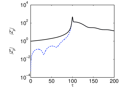
Figure 1: $~{}|Z_{p}^{+}|$ (solid black) and $~{}|Z_{p}^{-}|$ (dashed blue) vs time in log-linear scaling at: $Z_{p}^{+}(0)=1$, $Z_{p}^{-}(0)=0$, $Z_{s}^{+}(0)=0$, $Z_{s}^{-}(0)=0$, $\Omega_{A}=0.1$, $~{}k_{y}(0)/k_{x}=100$ and $k_{z}=0$.

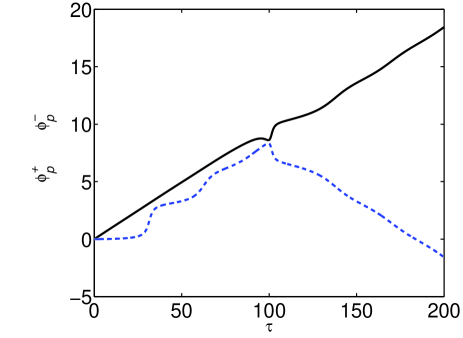
Figure 2: $~{}\phi_{p}^{+}$ (solid black) and $~{}\phi_{p}^{-}$ (dashed blue) vs time for the same parameters as in figure 1.

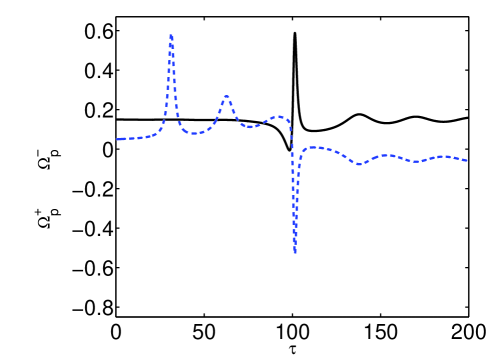
Figure 3: Instantaneous frequencies $\Omega_{p}^{+}$ (solid black) and $~{}\Omega_{p}^{-}$ (dashed blue) vs time for the same parameters as in figure 1.

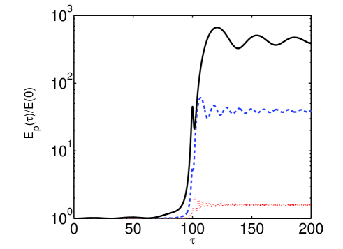
Figure 4: Normalized spectral energy of P-AWs, $E_{p}(\tau)/E(0)$, vs time in log-linear scaling for the same parameters as in figure 1, but at $\Omega_{A}=0.1$ (solid black), $~{}\Omega_{A}=0.3$ (dashed blue) and $~{}\Omega_{A}=1$ (dotted red).

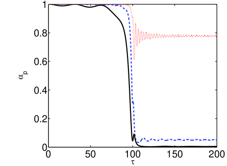
Figure 5: The imbalance degree of P-AWs, $\alpha_{p}=1-|Z_{p}^{-}|^{2}|Z_{p}^{+}|^{2}$, vs time for the same parameters as in figure 1, but at $~{}\Omega_{A}=0.1$ (solid black), $~{}\Omega_{A}=0.3$ (dashed blue) and $~{}\Omega_{A}=1$ (dotted red).

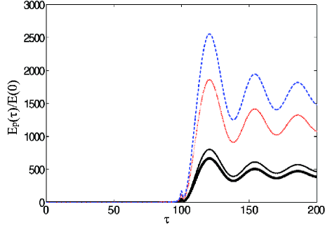
Figure 6: Normalized spectral energy of P-AWs, $E_{p}(\tau)/E(0)$, vs time in two-dimensional case ($k_{z}=0$, $Z_{s}^{\pm}=0$) at: $\Omega_{A}=0.1$, $~{}k_{y}(0)/k_{x}=100$, $Z_{p}^{+}(0)=1$ and $Z_{p}^{-}(0)=0$ (thick solid black), $Z_{p}^{-}(0)=1$ (solid black), $Z_{p}^{-}(0)=i$ (dashed blue), $Z_{p}^{-}(0)=-1$ (dotted red).

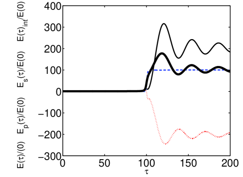
Figure 7: Normalized spectral energies: $E(\tau)/E(0)$ (thick solid black), $E_{p}(\tau)/E(0)$ (solid black), $E_{s}(\tau)/E(0)$ (dashed blue) and $E_{int}(\tau)/E(0)$ (dotted red) vs time at: $Z_{p}^{+}(0)=1$, $Z_{p}^{-}(0)=0$, $Z_{s}^{\pm}(0)=0$, $\Omega_{A}=0.1$, $~{}k_{y}(0)/k_{x}=100$ and $k_{z}/k_{x}=1$.

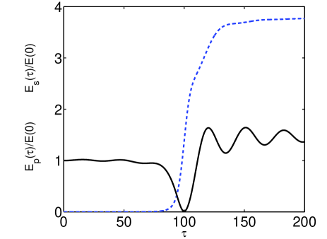
Figure 8: Normalized spectral energies of P-AWs and S-AWs, $E_{p}(\tau)/E(0)$ (solid black) and $E_{s}(\tau)/E(0)$ (dashed blue), vs time for the same parameters as in figure 7, but at $k_{z}/k_{x}=10$.

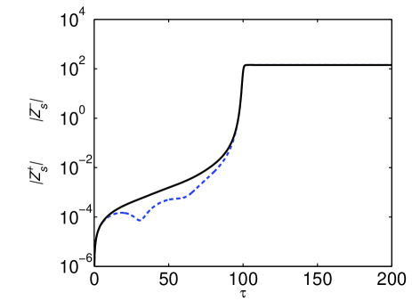
Figure 9: $~{}|Z_{s}^{+}|$ (solid black) and $~{}|Z_{s}^{-}|$ (dashed blue) vs time in log-linear scaling for the same parameters as in figure 7.

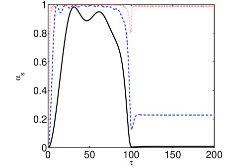
Figure 10: The imbalance degree of S-AWs, $\alpha_{s}=1-|Z_{s}^{-}|^{2}/|Z_{s}^{+}|^{2}$, vs time in log-linear scaling for the same parameters as in figure 7, but at $~{}\Omega_{A}=0.1$ (solid black), $~{}\Omega_{A}=0.3$ (dashed blue) and $~{}\Omega_{A}=1$ (dotted red).

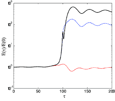
Figure 11: Normalized spectral energy, $E(\tau)/E(0)$, vs time in log-linear scaling for 2D and 3D cases for the same parameters as in figure 7, but at $k_{z}/k_{x}=0$ (solid), $k_{z}/k_{x}=1$ (dashed) and $k_{z}/k_{x}=10$ (dotted).

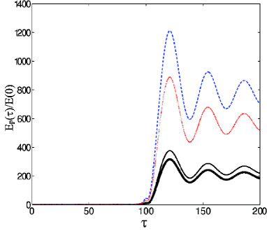
Figure 12: Normalized spectral energy of P-AWs, $E_{p}(\tau)/E(0)$, vs time at: $\Omega_{A}=0.1$, $~{}k_{y}(0)/k_{x}=100$, $k_{z}/k_{x}=1$, $Z_{s}^{\pm}(0)=0$, $Z_{p}^{+}(0)=1$ and $Z_{p}^{-}(0)=0$ (thick solid black), $Z_{p}^{-}(0)=1$ (solid black), $Z_{p}^{-}(0)=i$ (dashed blue), $Z_{p}^{-}(0)=-1$ (dotted red).

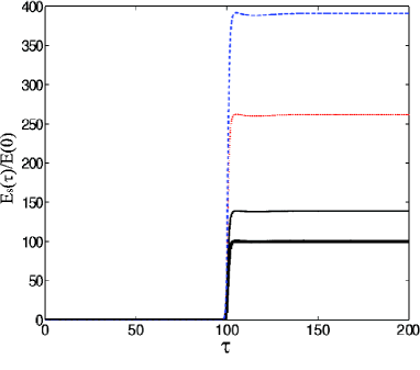
Figure 13: Normalized spectral energy of S-AWs, $E_{s}(\tau)/E(0)$, vs time at: $\Omega_{A}=0.1$, $~{}k_{y}(0)/k_{x}=100$, $k_{z}/k_{x}=1$, $Z_{s}^{\pm}(0)=0$, $Z_{p}^{+}(0)=1$ and $Z_{p}^{-}(0)=0$ (thick solid black), $Z_{p}^{-}(0)=1$ (solid black), $Z_{p}^{-}(0)=i$ (dashed blue), $Z_{p}^{-}(0)=-1$ (dotted red).

With the help of equations (2.13) and (2.14) and Figures 1-3 one can trace each stage of the evolution of the counter-propagating P-AW harmonic, which in fact, represents the overreflection phenomenon. Initially, as $Z_{p}^{-}(0)=0$, in (2.14) only the last rhs term is nonzero. So, the initial amplification and the dynamics of $Z_{p}^{-}(\tau)$ is due to the third term $\chi_{p}Z^{+}$. Therefore, the positive “instantaneous frequency” of $Z_{p}^{+}$ results in the positive “instantaneous frequency” of $Z_{p}^{-}$ (see figure 3). The growth of $|Z_{p}^{-}|$ is rapid, but algebraic (nonexponential). In the course of the evolution, $|Z_{p}^{-}|$ becomes almost equal to $|Z_{p}^{+}|$ (see figure 1 at $\tau\simeq\tau^{*}\equiv k_{y}(0)/k_{x}=100$). At the same time, the influence of the first and second rhs terms of equation (2.14) become appreciable, behavior of $\phi_{p}^{-}$ and $\Omega_{p}^{-}$ changes at $\tau\simeq\tau^{*}$ with $\Omega_{p}^{-}$ becoming negative and, as a result of all these, $Z_{p}^{-}$ is propagating opposite to $Z_{p}^{+}$. With further increase of time, $\Omega_{p}^{-}$ tends to $-\Omega_{A}$ and slightly varies around it. As for the dynamics of $Z_{p}^{+}$, the coupling (the last rhs term of equation 2.13) somewhat modifies its dynamics in the vicinity of $\tau\simeq\tau^{*}$, where $Z_{p}^{-}$ is already large and $\chi_{p}$ is not small too (while at $\tau\gg\tau^{*},~{}\chi_{p}\rightarrow 0$).

Figure 4 shows that, starting with a purely unidirectional P-AW harmonic, $Z_{p}^{-}(0)=0$, the perturbation energy increases and reaches a peak value at time $\tau\simeq\tau^{*}$. After that, the harmonic undergoes nearly periodic and damping oscillations around some plateau value of the energy. This plateau value increases with decreasing $\Omega_{A}$.

Figure 5 shows that the imbalance degree of the P-AW harmonic decreases with time (with the increase of the amplitudes), i.e., the energy propagating opposite to the $X$-axis approaches the energy propagating along the $X$-axis: for the case of $\Omega_{A}=1$, the harmonic remains imbalanced, for the case of $\Omega_{A}=0.3$ the imbalance degree tends to $0.05$, and for the case of $\Omega_{A}=0.1$, in fact, the harmonic becomes balanced with time.

When initially counter-propagating P-AW harmonics with equal amplitudes but different phases ($Z_{p}^{+}(0)=1$ and $Z_{p}^{-}(0)=1,i,-1$) are inserted, the dynamics is simpler. Amplitudes of the physical variables are equal to each other, $Z_{p}^{+}(\tau)=Z_{p}^{-}(\tau)$, according to equation (2.22), i.e., they are balanced from the beginning and their phase dynamics is quite trivial.

Figure 6 shows that the transient growth of perturbation energy is smaller in the case of initially imposed unidirectional P-AW harmonic than that in the case when equal amplitude counter-propagating P-AW harmonics are imposed. And, in the latter cases, the energy growth is maximum if the phases of the inserted harmonics differ from each other by $\pi/2~{}$ ($Z_{p}^{+}(0)=1$ and $Z_{p}^{-}(0)=i$).

3.2 Three-dimensional case

Figures 7-11 correspond to 3D cases when initially just unidirectional P-AW harmonic is imposed in the flow. Figures 12 and 13 – when initially counter-propagating P-AW harmonics are inserted with equal amplitudes but different phases.

In the 3D case, S-AWs become an active participant in the dynamics, however, the growth of P-AWs remains somewhat larger than the growth of S-AWs. Figure 7 shows the prevalence of P-AWs for $k_{z}/k_{x}=1$. (It is natural that this prevalence is more pronounced for $~{}k_{z}/k_{x}\ll 1$.) The transient growth of both waves substantially reduces with the further increase of the ratio $~{}k_{z}/k_{x}$ (see figure 8) and, consequently, SFHs with $~{}k_{z}/k_{x}\gg 1$ do not play any role in the dynamical processes.

In figure 9 we present the dynamics of $|Z_{s}^{+}|$ (solid black) and $|Z_{s}^{-}|$ (dashed blue) vs time in log-linear scaling for a small value of $\Omega_{A}$ ($\Omega_{A}=0.1$) and $k_{z}/k_{x}=1$ when, only $Z_{p}^{+}(0)$ is inserted in the flow (i.e., $Z_{p}^{-}(0),Z_{s}^{\pm}(0)=0$). In the beginning, $|Z_{s}^{+}|$ increases stronger than $|Z_{s}^{-}|$. However, in the course of the evolution, $|Z_{s}^{-}|$ becomes almost equal to $|Z_{s}^{+}|$. Figure 10 shows that with increase of the amplitudes, the imbalance degree of the S-AWs decreases with time for small $\Omega_{A}$ as it is for P-AWs (compare figures 5 and 10). S-AWs are imbalanced already at $\Omega_{A}\simeq 1$. However, the growth of S-AWs is negligible in the last case.

Figure 11 shows that, the growth of the total spectral energy is maximal for 2D case and decreases with the increase of $~{}k_{z}/k_{x}$. This result is somewhat unexpected/surprising, because in non-magnetized flows (i.e., in the simplest incompressible hydrodynamic constant shear flow) the transient growth of three-dimensional perturbations is generally stronger than transient growth of two-dimensional ones (e.g., see Chagelishvili et al., 1996; Moffatt, 1967; Farrell & Ioannou, 1993a; Bakas et al., 2001) and the dynamics of a non-magnetized system is determined by three-dimensional perturbations.

Figures 12 and 13 show that the energy growth is maximal if the phases of inserted SFHs differ from each other by $\pi/2$ (as in the 2D case). These figures also coincide with 7 for cases when phases of the initially inserted SFHs differ from each other – the transient growth of P-AW always prevails over the growth of S-AW. All energy dynamics plots (see figures 4,6,7,11-13) show that real transient growth takes place in the vicinity of $\tau\simeq\tau^{*}$ during the time interval $|\tau-\tau^{*}|\leq\Omega_{A}^{-1}$.

4 Summary and discussion

The proposed formalism provides a deeper insight into the physical mechanism underlying the overreflection phenomenon by allowing us to separate from each other physical processes associated with counter-propagating waves and to follow their interaction during the overreflection. Based on the presented analysis, the path to the overreflection is as follows. Initially an imposed on the shear flow pure $Z_{p}^{+}$ generates $Z_{p}^{-}$ due to the shear-induced linear coupling, that at first propagates in the same direction as $Z_{p}^{+}$. With time, $Z_{p}^{-}$ grows transiently and in the vicinity of $\tau\simeq\tau^{*}$ (at which $~{}k_{y}(\tau^{*})=0$) reverses the direction of propagation and becomes counter-propagating to $Z_{p}^{+}$. Both counter-propagating P-AWs SFHs exhibit transient growth that is appreciable at $\Omega_{A}<1$, $k_{z}/k_{x}\leq 1$ and $k_{y}(0)/k_{x}\gg 1$. As for S-AWs, its transient growth occurs due to the linear coupling of P-AW and S-AW, i.e. – is an indirect consequence of P-AW (i.e. $Z_{p}^{+}$ and $Z_{p}^{-}$) growth. At the same time, the growth of P-AWs somewhat prevails over the growth of S-AWs. It is obvious, that the dynamics has transient nature, as it should be – shear flow non-normality induced energy exchange processes are always transient (e.g., see Schmid, 2007). This statement is correct for constant in time shear flows. However, in periodic shear flows (i.e., when shear parameter is a periodic function of time), wave perturbations may grow exponentially in time. For instance, Zaqarashvili (2000); Zaqarashvili & Roberts (2002) studied the stability of periodic MHD shear flows, showing that the temporal behaviour of spatial Fourier harmonics of magnetosonic waves is governed by Mathieu’s equation. Consequently, the harmonics with the half frequency of the shear flow grow exponentially in time. Mathieu’s equation represent a single second order ordinary differential (wave) equation and describes counter-propagating waves of a single/physical variable. Consequently, possible dynamical processes between these waves (e.g., their coupling) are, in fact, left out of consideration. To get an additional information about the physics of the growth (e.g., to grasp the coupling between counter-propagating waves) one has to find “eigen-variable” for each wave component and, by this way, reduce Mathieu’s equation to the set of first order differential equations for individual counter-propagating wave (as it is done for the constant shear flows).

Evaluating the linear transient dynamics we use the concept of energy. Of course, when calculating energy - the quantity of the second order in the wave amplitude - causes dissatisfaction associated with the known fact: it is obviously necessary to take into account changes in the mean parameters of the environment and, in particular, the wave-induced flow (Stepanyants & Fabrikant, 1989). In this case, there is an ambiguous field separation of the physical variables in the wave field and the medium field. These issues are rather complicated and analysis continues to this day. For example, in the MHD context, theory for the wave and background stress energy tensors is developed based on the exact Lagrangian map in Webb et al. (2005). We do not go into this debate, but, only aim to get a feeling of the dynamics of quadratic forms of physical variables. Therefore, we introduced the concept of energy in solving the linearized problems as it is usually accepted in hydrodynamic and magnetodynamic flow studies (Stepanyants & Fabrikant, 1989).

Maximal transient growth (and overreflection) of the wave energy occurs in the 2D limit (at $k_{z}=0$). Consequently, the dynamics of the MHD flow should be defined mainly by SFHs with $k_{z}/k_{x}\ll 1$. At the same time, the transient growth of the both, P- and S-Alfv${\rm\acute{e}}$n wave modes increases with decreasing $\Omega_{A}$. If initially only unidirectional P-AW harmonic is imposed in the flow, the imbalance degree decreases with the decrease of $\Omega_{A}$ and the waves become already balanced at $\Omega_{A}=0.1$. If initially counter-propagating P-AW harmonics with equal amplitudes are imposed, they maintain the balance irrespective of the initial phase. Because of the condition $\Omega_{A}\sim k_{x}$, SFHs having smaller $k_{x}$ exhibit stronger growth. Finally, one can conclude, that the dynamical processes should be defined by waves having small $k_{x}$ and $k_{z}$, i.e. long streamwise and spanwise wavelengthes, $\lambda_{x},\lambda_{z}\gg V_{A}/S$.

4.1 Impact of the transient growth on the character of nonlinear cascade processes

The described linear dynamics is expected to have significant nonlinear consequences. The point is that the linear transient processes are mainly defined by coefficients $\chi_{p}$ of equations (2.13) and (2.14). The coefficients introduce dependency of the transient growth on the ratio $k_{x}k_{y}(\tau)/k^{2}(\tau)$. Consequently, the transient growth depends not on the value but on the orientation of wavevector and takes place when $|\chi_{p}(\tau)|\geq\Omega_{A}$, i.e. when $|k_{y}(\tau)/k_{x}|\leq\Omega_{A}^{-1}$. As it is outlined at the end of the previous section, this happens in the vicinity of $\tau\simeq\tau^{*}$ during the time interval $|\tau-\tau^{*}|\leq\Omega_{A}^{-1}$ (see figures 4,6,7,11-13). It is obvious, that the linear transient processes are highly anisotropic in wavenumber plane. A similar anisotropy exists in hydrodynamic shear flows Horton et al. (see for details 2010). The anisotropy changes classical view on the nonlinear cascade processes: classically, the net action of nonlinear (turbulent) processes is interpreted as either a direct or inverse cascade. However, as it is shown in Horton et al. (2010), in hydrodynamic nonuniform/shear flows, the dominant process is a nonlinear redistribution over wavevector angles of perturbation spatial Fourier harmonics. This anisotropic transfers of spectral energy in the wavenumber space has been coined as nonlinear transverse redistribution (NTR), one can also say – “nonlinear transverse cascade”.

NTR redistributes perturbation harmonics over different quadrants of the wavenumber plane (e.g., from quadrants where $k_{x}k_{y}>0$ to quadrants where $k_{x}k_{y}<0$ or vice versa) and the interplay of this nonlinear redistribution with linear phenomena (transient growth) becomes intricate: it can realize either positive or negative feedback. In the case of positive feedback, the nonlinearity repopulates transiently growing perturbations and contributes to the self-sustenance of perturbations. Consequently, NTR naturally appears as a possible cornerstone of the bypass scenario of turbulence.

The similarity of the anisotropy of the transient growth in the hydrodynamic and our MHD cases hints at the similarity of nonlinear processes. In other words, the transverse cascade should also be inherent to MHD shear flows. Therefore, the conventional characterization of MHD turbulence in terms of direct and inverse cascades, which ignores the transverse cascade, can be misleading for MHD shear flow turbulence. In principal, the nonlinear transverse cascade can repopulate the transiently growing wave SFHs in a MHD shear flow and can acquire a vital role of ensuring the self-sustenance of the waves. To verify these, consistent with the bypass concept, processes in MHD shear flows, we already simulated nonlinear dynamics of the considered here flow system in 2D limit (Mamatsashvili et al., 2014). The performed direct numerical simulations show the existence of subcritical transition to turbulence even in the 2D case, i.e., show the vitality of the bypass transition to turbulence for the simplest (spectrally stable) plane MHD flow. The minimal/critical Reynolds number of the subcritical transition turned out to be about $5000$, i.e. larger than for the hydrodynamic Couette flow, where $Re_{cr}\sim 350$. At the same time, in the hydrodynamic case, the transition occurs just in the 3D case, while in the simplest MHD flow, the subcritical transition and self-sustenance of turbulence occurs in the 2D case too.

Discussing the character of nonlinear cascade processes, finally, one has to present the generalising view.

MHD turbulence phenomenon is ubiquitous in nature and is very important in engineering/industrial applications. So, it is natural that there is an enormous amount of research devoted to it, starting with seminal papers Iroshnikov (1963) and Kraichnan (1965) and their extensions Goldreich & Sridhar (1995); Boldyrev (2005). To date, the main trends, including cases of forced, freely decaying and with background magnetic field MHD turbulence, established over decades are thoroughly analyzed in a number of review articles and books (see e.g., Biskamp, 2003; Mininni, 2011; Brandenburg & Lazarian, 2013). Most of such an analysis commonly focuses on turbulence dynamics in wavenumber/Fourier space. However, the case of MHD turbulence in smooth shear flows involves fundamental novelties: the energy-supplying process for turbulence is the flow nonnormality induced linear transient growth. The latter anisotropically injects energy into turbulence over a broad range of lengthscales, consequently, rules out the inertial range of the activity of nonlinearity and leads to complex interplay of linear and nonlinear processes (Mamatsashvili et al., 2014). These circumstances give rise to new type of processes in the turbulence dynamics that are not accounted for in the main trends of MHD turbulence research.

The essence of the view is the following: anisotropic linear processes lead to anisotropy of nonlinear processes. Specifically, the nonlinear transverse cascade (that is anisotropic by definition) is the result of only anisotropic linear coupling/reflection. For instance, there is a number of papers addressing linear wave reflection that is caused by parallel gradients of density/magnetic field (e.g., Velli et al., 1989; Matthaeus et al., 1999; Dmitruk et al., 2002; Verdini et al., 2012; Perez & Chandran, 2013). However, this kind of reflection, due to the absence of the above noted anisotropy in wavenumber space, should not lead to the nonlinear transverse cascade. A flow configuration, similar to our magnetized shear flow, is considered by Hollweg et al. (2013), addressing the wave reflection. The difference is in the value of beta parameter – we consider incompressible waves in high-beta plasma, while, that paper considers compressible waves in low-beta plasma. The participants of the linear dynamics are different, however, in the both cases, transient liner processes/coupling/growth are anisotropic. Consequently, the nonlinear transverse cascade should also be important for the range of parameters considered in Hollweg et al. (2013).

4.2 On application of the proposed approach of the overreflection to more complex shear flow systems

Finally, we would like to stress that the present scenario and mathematical formalism of the overreflection phenomenon is easily applicable to more complex shear flow systems, including widely discussed cases of overreflection of spiral-density waves in astrophysical discs and of internal-gravity waves in stably stratified atmospheres. The proposed approach describes each (counter-propagating) wave component by its generalized eigen variable. In the considered here MHD flow, fortunately, one can use Els$\ddot{a}$sser variables (see equation 2.12) or its renormalized version (see equation 2.23) as the generalized eigen variables. This fact has actually simplified our analysis. As for more complex shear flow systems, there appears to be some difficulty in finding generalized eigen variable and construction of fist order differential equations for each counter-propagating wave. The difficulty is due to the fact that in complex flow systems “nominal frequency” may depend on the varying/shearwise wavenumber and, consequently, on time (e.g., as the “nominal frequency” of internal-gravity waves), while in our case considered here Alfv${\rm\acute{e}}$n waves, the “nominal frequency” (Alfv${\rm\acute{e}}$n frequency) does not depend on the shearwise wavenumber and is constant. However, this is not a fundamental difficulty – it requires just a bit of complicated calculations and gives somewhat bulky coefficients in dynamical equations. So, to apply the proposed mathematical approach, one has to find eigen variables of the waves in the shearless limit, then generalize these eigen variables for the non-zero shear case and write dynamic equations for them. This procedure gives the corresponding set of easily foreseeable, coupled first order ordinary differential equations for each counter-propagating wave.

5 acknowledgment

The authors are grateful to Dr. George Mamatsashvili for valuable help in the preparing of the final version of the manuscript. This work was supported in part by GNSF grant 31/14.

References

- Baggett et al. (1995) Baggett, J, Driscoll, T & Trefethen, L 1995 A mostly linear model of transition to turbulence. Phys. Fluids 7, 833–538.
- Bakas et al. (2001) Bakas, N, Ioannou, P & Kefaliakos, G 2001 The emergence of coherent structures in stratified shear flow. J. Atmos. Sci. 58, 2790–2806.
- Biskamp (2003) Biskamp, D 2003 Magnetohydrodynamic turbulence. Cambridge University Press.
- Boldyrev (2005) Boldyrev, S 2005 On the spectrum of magnetohydrodynamic turbulence. Astrophys. J. Letters 626, L37–L40.
- Brandenburg & Lazarian (2013) Brandenburg, A & Lazarian, A 2013 Astrophysical hydromagnetic turbulence. Space Science Reviews 178, 163–200.
- Chagelishvili et al. (1996) Chagelishvili, G, Chanishvili, R & Lominadze, J 1996 Physics of the amplification of vortex disturbances in shear flows. JETP Lett. 63, 543–549.
- Chagelishvili et al. (1997a) Chagelishvili, G, Chanishvili, R, Lominadze, J & Tevzadze, A 1997a Magnetohydrodynamic waves linear evolution in parallel shear flows: Amplification and mutual transformations. Phys. Plasmas 5, 259–269.
- Chagelishvili et al. (1997b) Chagelishvili, G, Tevzadze, A, Bodo, G & Moiseev, S 1997b Linear mechanism of wave emergence from vortices in smooth shear flows. Phys. Rev. Lett. 79, 3178–3121.
- Dmitruk et al. (2002) Dmitruk, P, Matthaeus, W, Milano, L, Oughton, S, Zank, G & Mullan, D 2002 Coronal heating distribution due to low-frequency, wave-driven turbulence. Astrophisical J. 575, 571–577.
- Eckhardt et al. (2007) Eckhardt, B, Schneider, T, Hof, B & Westerweel, J 2007 Turbulence transition in pipe flow. Annu. Rev. Fluid Mech. 39, 447–468.
- Farrell & Ioannou (1993a) Farrell, B & Ioannou, P 1993a Optimal excitation of three-dimensional perturbations in viscous constant shear flow. Phys. Fluids A 5, 1390–1400.
- Farrell & Ioannou (1993b) Farrell, B & Ioannou, P 1993b Stochastic forcing of perturbation variance in unbounded shear and deformation flows. J. Atmos. Sci. 50, 200–211.
- Goldreich & Sridhar (1995) Goldreich, P. & Sridhar, S. 1995 Toward a theory of interstellar turbulence. 2: Strong alfvenic turbulence. Astrophysical J. 438, 763–775.
- Goldreich & Tremaine (1978) Goldreich, P. & Tremaine, S. 1978 The excitation and evolution of density waves. Astrophysical J. 222, 850–858.
- Goldreich & Tremaine (1979) Goldreich, P. & Tremaine, S. 1979 The excitation of density waves at the lindblad and corotation resonances by an external potential. Astrophysical J. 233, 857–871.
- Grossmann (2000) Grossmann, S. 2000 The onset of shear flow turbulence. Rev. Mod. Phys. 72, 603–618.
- Heinemann & Olbert (1980) Heinemann, M. & Olbert, S. 1980 Non-wkb alfvn waves in the solar wind. J. Geophysical Research: Space Physics 85, 1311–1327.
- Hollweg & Kaghashvili (2012) Hollweg, J. & Kaghashvili, E. 2012 Alfvn waves in shear flows revisited. Astrophysical J. 744, 114–118.
- Hollweg et al. (2013) Hollweg, J, Kaghashvili, E & Chandran, B 2013 Velocity-shear induced mode coupling in the solar atmospere and solar wind: implication for plasma heating and mhd turbulence. Astrophisical J. 769, 142–152.
- Horton et al. (2010) Horton, W, Kim, J.-H, Chagelishvili, G, Bowman, J & Lominadze, J 2010 Angular redistribution of nonlinear perturbations: A universal feature of nonuniform flows. Phys. Rev. E. 81, id. 066304.
- Iroshnikov (1963) Iroshnikov, P. 1963 Turbulence of a conducting fluid in a strong magnetic field. Sov. Astron. 7, 566–571.
- Kraichnan (1965) Kraichnan, R. 1965 Inertial-range spectrum of hydromagnetic turbulence. Phys. Fluids 8, 1385–1387.
- Lindzen & Barker (1985) Lindzen, R. S. & Barker, J. 1985 Instability and wave over-reflection in stably stratified shear flow. J. Fluid Mechanics 151, 189–217.
- Mamatsashvili et al. (2014) Mamatsashvili, G, Gogichaishvili, D, Chagelishvili, G & Horton, W 2014 Nonlinear transverse cascade and two-dimensional mhd subcritical turbulence in plane shear flows. in preparation .
- Matthaeus et al. (1999) Matthaeus, W, Zank, G, Oughton, S, Mullan, D & Dmitruk, P 1999 Coronal heating by magnetohydrodynamic turbulence driven by reflected low-frequency waves. Astrophisical J. 523, L93–L96.
- Mininni (2011) Mininni, P. D. 2011 Scale interactions in magnetohydrodynamic turbulence. Annual Review of Fluid Mechanics 43, 377–397.
- Moffatt (1967) Moffatt, H. K. 1967 The interaction of turbulence with strong wind shear. pp. 139–156.
- Perez & Chandran (2013) Perez, J & Chandran, B 2013 Direct numerical simulations of reflection-driven, mhd turbulence from the sun to the alfvn critical point. Astrophisical J. 776, 124–140.
- Reddy & Henningson (1993) Reddy, S. & Henningson, D. 1993 Energy growth in viscous channel flows. J. Fluid Mech. 252, 209–238.
- Schmid (2007) Schmid, P. 2007 Nonmodal stability theory. Annu. Rev. Fluid Mech. 39, 129–162.
- Stepanyants & Fabrikant (1989) Stepanyants, Yu. & Fabrikant, A. 1989 Reviews of topical problems: Propagation of waves in hydrodynamic shear flows. Soviet Physics Uspekhi 32, 783–805.
- Trefethen et al. (1993) Trefethen, L, Trefethen, A, Reddy, S & Driscoll, T 1993 Hydrodynamic stability without eigenvalues. Science 261, 578–584.
- Velli et al. (1989) Velli, M, Grappin, R & Mangeney, A 1989 Turbulenct cascade of incompressible unidirectional alfvn waves in the interplanetary medium. Phys. Rev. Lett. 63, 1807–1810.
- Verdini et al. (2012) Verdini, A, Grappin, R, Pinto, R & Velli, M 2012 On the origin of the spectrum in the solar wind magnetic field. Astrophisical J. Lett. 750, L33–L37.
- Webb et al. (2005) Webb, G, Zank, G, Kaghashvili, E & Ratkiewicz, R 2005 Magnetohydrodynamic waves in non-uniform flows i: a variational approach. Journal of Plasma Physics 71, 785–809.
- Yoshida (2005) Yoshida, Z. 2005 Kinetic theory for non-hermitian dynamics of waves in shear flow. Phys. Plasmas 12, 024503–024503–3.
- Zaqarashvili (2000) Zaqarashvili, T. 2000 Parametric resonance in ideal magnetohydrodynamics. Phys. Rev. E 62, 2745–2753.
- Zaqarashvili & Roberts (2002) Zaqarashvili, T. & Roberts, B. 2002 Swing wave-wave interaction: Coupling between fast magnetosonic and alfvn waves. Phys. Rev. E 66, id. 026401.