Nuclear Spin Dynamics in Double Quantum Dots: Multi-Stability, Dynamical Polarization, Criticality and Entanglement

Abstract

We theoretically study the nuclear spin dynamics driven by electron transport and hyperfine interaction in an electrically defined double quantum dot in the Pauli-blockade regime. We derive a master-equation-based framework and show that the coupled electron-nuclear system displays an instability towards the buildup of large nuclear spin polarization gradients in the two quantum dots. In the presence of such inhomogeneous magnetic fields, a quantum interference effect in the collective hyperfine coupling results in sizable nuclear spin entanglement between the two quantum dots in the steady state of the evolution. We investigate this effect using analytical and numerical techniques, and demonstrate its robustness under various types of imperfections.

I Introduction

The prospect of building devices capable of quantum information processing (QIP) has fueled an impressive race to implement well-controlled two-level quantum systems (qubits) in a variety of physical settings.zoller05 For any such system, generating and maintaining entanglement—one of the most important primitives of QIP—is a hallmark achievement. It serves as a benchmark of experimental capabilities and enables essential information processing tasks such as the implementation of quantum gates and the transmission of quantum information.nielsen00

In the solid state, electron spins confined in electrically defined semiconductor quantum dots have emerged as a promising platform for QIP: hanson07 ; chekhovich13 ; awschalom02 ; loss98 Essential ingredients such as initialization, single-shot readout, universal quantum gates and, quite recently, entanglement have been demonstrated experimentally.nowack11 ; petta05 ; shulman12 ; koppens06 ; koppens05 ; nowack07 In this context, nuclear spins in the surrounding semiconductor host environment have attracted considerable theoreticalkhaetskii02 ; erlingsson01 ; schliemann03 ; coish04 ; coish08 ; cywinski09 ; merkulov02 and experimentalvink09 ; bluhm10 ; foletti09 ; johnson05 ; ono04 ; ono02 attention, as they have been identified as the main source of electron spin decoherence due to the relatively strong hyperfine (HF) interaction between the electronic spin and $N\sim 10^{6}$ nuclei.chekhovich13 However, it has also been noted that the nuclear spin bath itself, with nuclear spin coherence times ranging from hundreds of microseconds to a millisecond,takahashi11 ; chekhovich13 could be turned into an asset, for example, as a resource for quantum memories or quantum computation. taylor03 ; taylor04 ; witzel07 ; cappellaro09 ; kurucz09 Since these applications require yet unachieved control of the nuclear spins, novel ways of understanding and manipulating the dynamics of the nuclei are called for. The ability to control and manipulate the nuclei will open up new possibilities for nuclear spin-based information storage and processing, but also directly improve electron spin decoherence timescales.rudner07 ; rudner07b ; rudner11a

Dissipation has recently been identified as a novel approach to control a quantum system, create entangled states or perform quantum computing tasks.verstraete09 ; diehl08 ; sanchez13 ; tomadin12 ; poyatos96 This is done by properly engineering the continuous interaction of the system with its environment. In this way, dissipation—previously often viewed as a vice from a QIP perspective—can turn into a virtue and become the driving force behind the emergence of coherent quantum phenomena. The idea of actively using dissipation rather than relying on coherent evolution extends the traditional DiVincenzo criteriadivincenzo00 to settings in which no unitary gates are available; also, it comes with potentially significant practical advantages, as dissipative methods are inherently robust against weak random perturbations, allowing, in principle, to stabilize entanglement for arbitrary times. Recently, these concepts have been put into practice experimentally in different QIP architectures, namely atomic ensembles,muschik11 trapped ionslin13 ; barreiro11 and superconducting qubits.shankar13

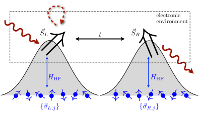
Figure 1: (color online). Schematic illustration of the DQD system under study. Two nuclear spin ensembles are hyperfine-coupled to the electronic subsytem; due to various fast coherent (double-arrow) and incoherent processes (arrows) the latter settles to a quasisteady state on a timescale shorter than the nuclear dynamics.

Here, we apply these ideas to a quantum dot system and investigate a scheme for the deterministic generation of steady-state entanglement between the two spatially separated nuclear spin ensembles in an electrically defined double quantum dot (DQD), operated in the Pauli-blockade regime.ono02 ; hanson07 Expanding upon our proposal presented in Ref.schuetz13 , we develop in detail the underlying theoretical framework, and discuss in greater depth the coherent phenomena emerging from the hyperfine coupled electron and nuclear dynamics in a DQD in spin blockade regime. The analysis is based on the fact that the electron spins evolve rapidly on typical timescales of the nuclear spin dynamics. This allows us to derive a coarse-grained quantum master equation for the nuclear spins only, disclosing the nuclei as the quantum system coupled to an electronic environment with an exceptional degree of tunability; see Fig.  1 for a schematic illustration. This approach provides valuable insights by building up a straightforward analogy between mesoscopic solid-state physics and a generic setting in quantum optics (compare, for example, Ref.muschik11 ): The nuclear spin ensemble can be identified with an atomic ensemble, with individual nuclear spins corresponding to the internal levels of a single atom and electrons playing the role of photons.schuetz12

Our theoretical analysis goes beyond this simple analogy by incorporating nonlinear, feedback-driven effects resulting from a backaction of the effective magnetic field generated by the nuclei (Overhauser shift) on the electron energy levels. In accordance with previous theoreticalrudner07 ; rudner11a ; rudner11b ; jouravlev96 ; lopez-moniz11 ; economou13 ; danon09b ; lunde13 and experimentalbaugh07 ; petta08 ; kobayashi11 ; koppens05 ; ono04 ; barthel12 observations, this feedback mechanism is shown to lead to a rich set of phenomena such as multistability, criticality, and dynamic nuclear polarization (DNP). In our model, we study the nuclear dynamics in a systematic expansion of the master equation governing the evolution of the combined electron-nuclear system, which allows us efficiently trace out the electronic degrees of freedom yielding a compact dynamical equation for the nuclear system alone. This mathematical description can be understood in terms of the so-called slaving principle: The electronic subsystem settles to a quasisteady state on a timescale much faster than the nuclear dynamics, and creates an effective environment with tunable properties for the nuclear spins. Consequently, we analyze the nuclear dynamics subject to this artificial environment. Feedback effects kick in as the generated nuclear spin polarization acts back on the electronic subsystem via the Overhauser shift changing the electronic quasisteady state. We derive explicit expressions for the nuclear steady state which allows us to fully assess the nuclear properties in dependence on the external control parameters. In particular, we find that, depending on the parameter regime, the polarization of the nuclear ensemble can show two distinct behaviors: The nuclear spins either saturate in a dark state without any nuclear polarization or, upon surpassing a certain threshold gradient, turn self-polarizing and build up sizable Overhauser field differences. Notably, the high-polarization stationary states feature steady-state entanglement between the two nuclear spin ensembles, even though the electronic quasisteady state is separable, underlining the very robustness of our scheme against electronic noise.

To analyze the nuclear spin dynamics in detail, we employ different analytical approaches, namely a semiclassical calculation and a fully quantum mechanical treatment. This is based on a hierarchy of timescales: While the nuclear polarization process occurs on a typical timescale of $\tau_{\mathrm{pol}}\gtrsim 1\mathrm{s}$, the timescale for building up quantum correlations $\tau_{\mathrm{gap}}$ is collectivelyschuetz12 enhanced by a factor $N\sim 10^{5}-10^{6}$; i.e., $\tau_{\mathrm{gap}}\approx\left(3-30\right)\mu\mathrm{s}$. Since nuclear spins dephase due to internal dipole-dipole interactions on a timescale of $\tau_{\mathrm{dec}}\approx\left(0.1-1\right)\mathrm{ms}$,gullans10 ; takahashi11 ; chekhovich13 our system exhibits the following separation of typical timescales: $\tau_{\mathrm{pol}}\gg\tau_{\mathrm{dec}}\gg\tau_{\mathrm{gap}}$. While the first inequality allows us to study the (slow) dynamics of the macroscopic semiclassical part of the nuclear fields in a mean-field treatment (which essentially disregards quantum correlations) on long timescales, based on the second inequality we investigate the generation of (comparatively small) quantum correlations on a much faster timescale where we neglect decohering processes due to internal dynamics among the nuclei. Lastly, numerical results complement our analytical findings and we discuss in detail detrimental effects typically encountered in experiments.

This paper is organized as follows. Section II introduces the master-equation-based theoretical framework. Based on a simplified model, in Sec. III we study the coupled electron nuclear dynamics. Using adiabatic elimination techniques, we can identify two different regimes as possible fixed points of the nuclear evolution which differ remarkably in their nuclear polarization and entanglement properties. Subsequently, in Sec. IV the underlying multi-stability of the nuclear system is revealed within a semiclassical model. Based on a self-consistent Holstein-Primakoff approximation, in Sec. V we study in great detail the nuclear dynamics in the vicinity of a high-polarization fixed point. This analysis puts forward the main result of our work, the steady-state generation of entanglement between the two nuclear spin ensembles in a DQD. Within the framework of the Holstein-Primakoff analysis, Sec. VI highlights the presence of a dissipative phase transition in the nuclear spin dynamics. Generalizations of our findings to inhomogeneous hyperfine coupling and other weak undesired effects are covered in Sec. VII. Finally, in Sec. VIII we draw conclusions and give an outlook on possible future directions of research.

II The System

This section presents a detailed description of the system under study, a gate-defined double quantum dot (DQD) in the Pauli-blockade regime. To model the dynamics of this system, we employ a master equation formalism.schuetz12 This allows us to study the irreversible dynamics of the DQD coupled to source and drain electron reservoirs. By tracing out the unobserved degrees of freedom of the leads, we show that—under appropriate conditions to be specified below—the dynamical evolution of the reduced density matrix of the system $\rho$ can formally be written as

$$\dot{\rho}=\underset{\leavevmode\hbox to14.18pt{\vbox to14.18pt{\text{[drawing]}}}}{\underbrace{-i\left[H_{\mathrm{el}},\rho\right]+\mathcal{V}\rho+\mathcal{L}_{\Gamma}\rho}}+\underset{\leavevmode\hbox to14.18pt{\vbox to14.18pt{\text{[drawing]}}}}{\underbrace{\mathcal{L}_{\pm}\rho+\mathcal{L}_{\mathrm{deph}}\rho}},$$ (1)

Here, $H_{\mathrm{el}}$ describes the electronic degrees of freedom of the DQD in the relevant two-electron regime, $\mathcal{V}$ refers to the coherent hyperfine coupling between electronic and nuclear spins and $\mathcal{L}_{\Gamma}$ is a Liouvillian of Lindblad form describing electron transport in the spin-blockade regime. The last two terms labeled by account for different physical mechanisms such as cotunneling, spin-exchange with the leads or spin-orbital coupling in terms of effective dissipative terms in the electronic subspace.

II.1 Microscopic Model

We consider an electrically defined DQD in the Pauli-blockade regime.hanson07 ; ono02 Microscopically, our analysis is based on a two-site Anderson Hamiltonian: Due to strong confinement, both the left and right dot are assumed to support a single orbital level $\epsilon_{i}\left(i=L,R\right)$ only which can be Zeeman split in the presence of a magnetic field and occupied by up to two electrons forming a localized spin singlet. For now, excited states, forming on-site triplets that could lift spin-blockade, are disregarded, since they are energetically well separated by the singlet-triplet splitting $\Delta_{\mathrm{st}}\gtrsim 400\mu\mathrm{eV}$.hanson07 Cotunneling effects due to energetically higher lying localized triplet states will be addressed separately below.

Formally, the Hamiltonian for the global system $\mathcal{H}$ can be decomposed as

$$\mathcal{H}=H_{\mathrm{DQD}}+H_{B}+H_{T},$$ (2)

where $H_{B}$ refers to two independent reservoirs of non-interacting electrons, the left $\left(L\right)$ and right $\left(R\right)$ lead, respectively,

$$H_{B}=\sum_{i,k,\sigma}\epsilon_{ik}c_{ik\sigma}^{\dagger}c_{ik\sigma},$$ (3)

with $i=L,R$, $\sigma=\uparrow,\downarrow$ and $H_{T}$ models the coupling of the DQD to the leads in terms of the tunnel Hamiltonian

$$H_{T}=\sum_{i,k,\sigma}T_{i}d_{i\sigma}^{\dagger}c_{ik\sigma}+\mathrm{h.c.}.$$ (4)

The tunnel matrix element $T_{i}$, specifying the transfer coupling between the leads and the system, is assumed to be independent of momentum $k$ and spin $\sigma$ of the electron. The fermionic operator $c_{ik\sigma}^{\dagger}\left(c_{ik\sigma}\right)$ creates (annihilates) an electron in lead $i=L,R$ with wavevector $k$ and spin $\sigma=\uparrow,\downarrow$. Similarly, $d_{i\sigma}^{\dagger}$ creates an electron with spin $\sigma$ inside the dot in the orbital $i=L,R$. Accordingly, the localized electron spin operators are

$$\vec{S}_{i}=\frac{1}{2}\sum_{\sigma,\sigma^{\prime}}d_{i\sigma}^{\dagger}\vec{\sigma}_{\sigma\sigma^{\prime}}d_{i\sigma^{\prime}},$$ (5)

where $\vec{\sigma}$ refers to the vector of Pauli matrices. Lastly,

$$H_{\mathrm{DQD}}=H_{S}+H_{t}+V_{\mathrm{HF}}$$ (6)

describes the coherent electron-nuclear dynamics inside the DQD. In the following, $H_{S}$, $H_{t}$ and $V_{\mathrm{HF}}$ are presented. First, $H_{S}$ accounts for the bare electronic energy levels in the DQD and Coulomb interaction terms

$$H_{S}=\sum_{i\sigma}\epsilon_{i\sigma}n_{i\sigma}+\sum_{i}U_{i}n_{i\uparrow}n_{i\downarrow}+U_{LR}n_{L}n_{R},$$ (7)

where $U_{i}$ and $U_{LR}$ refer to the on-site and interdot Coulomb repulsion; $n_{i\sigma}=d_{i\sigma}^{\dagger}d_{i\sigma}$ and $n_{i}=n_{i\uparrow}+n_{i\downarrow}$ are the spin-resolved and total electron number operators, respectively. Typical values are $U_{i}\approx 1-4m\mathrm{eV}$ and $U_{LR}\approx 200\mu\mathrm{eV}$.hayashi03 ; hanson07 ; ono02 Coherent, spin-preserving interdot tunneling is described by

$$H_{t}=t\sum_{\sigma}d_{L\sigma}^{\dagger}d_{\mathrm{R\sigma}}+\mathrm{h.c.}$$ (8)

Spin-blockade regime.—By appropriately tuning the chemical potentials of the leads $\mu_{i}$, one can ensure that at maximum two conduction electrons reside in the DQD.hanson07 ; sanchez13 Moreover, for $\epsilon_{R\sigma}<\mu_{R}$ the right dot always stays occupied. In what follows, we consider a transport setting where an applied bias between the two dots approximately compensates the Coulomb energy of two electrons occupying the right dot, that is $\epsilon_{L}\approx\epsilon_{R}+U_{R}-U_{LR}$. Then, a source drain bias across the DQD device induces electron transport via the cycle $\left(0,1\right)\rightarrow\left(1,1\right)\rightarrow\left(0,2\right)$. Here, $\left(m,n\right)$ refers to a configuration with $m\left(n\right)$ electrons in the left (right) dot, respectively. In our Anderson model, the only energetically accessible $\left(0,2\right)$ state is the localized singlet, referred to as $\left|S_{02}\right\rangle=d_{R\uparrow}^{\dagger}d_{R\downarrow}^{\dagger}\left|0\right\rangle$. As a result of the Pauli principle, the interdot charge transition $\left(1,1\right)\rightarrow\left(0,2\right)$ is allowed only for the $\left(1,1\right)$ spin singlet $\left|S_{11}\right\rangle=\left(\left|\Uparrow\Downarrow\right\rangle-\left|\Downarrow\Uparrow\right\rangle\right)/\sqrt{2}$, while the spin triplets $\left|T_{\pm}\right\rangle$ and $\left|T_{0}\right\rangle=\left(\left|\Uparrow\Downarrow\right\rangle+\left|\Downarrow\Uparrow\right\rangle\right)/\sqrt{2}$ are Pauli blocked. Here, $\left|T_{+}\right\rangle=\left|\Uparrow\Uparrow\right\rangle$, $\left|T_{-}\right\rangle=\left|\Downarrow\Downarrow\right\rangle$, and $\left|\sigma\sigma^{\prime}\right\rangle=d_{L\sigma}^{\dagger}d_{R\sigma^{\prime}}^{\dagger}\left|0\right\rangle$. For further details on how to realize this regime we refer to Appendix A.

Hyperfine interaction.—The electronic spins $\vec{S}_{i}$ confined in either of the two dots $\left(i=L,R\right)$ interact with two different sets of nuclear spins $\left\{\sigma_{i,j}^{\alpha}\right\}$ in the semiconductor host environment via hyperfine (HF) interaction. It is dominated by the isotropic Fermi contact term schliemann03 given by

$$H_{\mathrm{HF}}=\frac{a_{\mathrm{hf}}}{2}\sum_{i=L,R}\left(S_{i}^{+}A_{i}^{-}+S_{i}^{-}A_{i}^{+}\right)+a_{\mathrm{hf}}\sum_{i=L,R}S_{i}^{z}A_{i}^{z}.$$ (9)

Here, $S_{i}^{\alpha}$ and $A_{i}^{\alpha}=\sum_{j}a_{i,j}\sigma_{i,j}^{\alpha}$ for $\alpha=\pm,z$ denote electron and collective nuclear spin operators. The coupling coefficients $a_{i,j}$ are proportional to the weight of the electron wavefunction at the $j$th lattice site and define the individual unitless HF coupling constant between the electron spin in dot $i$ and the $j$th nucleus. They are normalized such that $\sum_{j=1}^{N_{i}}a_{i,j}=N$, where $N=\left(N_{1}+N_{2}\right)/2\sim 10^{6}$; $a_{\mathrm{hf}}$ is related to the total HF coupling strength $A_{\mathrm{HF}}\approx 100\mu\mathrm{eV}$ via $a_{\mathrm{hf}}=A_{\mathrm{HF}}/N$ and $g_{\mathrm{hf}}=A_{\mathrm{HF}}/\sqrt{N}\approx 0.1\text{$\mu\mathrm{eV}$}$ quantifies the typical HF interaction strength. The individual nuclear spin operators $\sigma_{i,j}^{\alpha}$ are assumed to be spin-$\frac{1}{2}$ for simplicity. We neglect the nuclear Zeeman and dipole-dipole terms which will be slow compared to the system’s dynamicsschliemann03 ; these simplifications will be addressed in more detail in Sec. VII.

The effect of the hyperfine interaction can be split up into a perpendicular component

$$H_{\mathrm{ff}}=\frac{a_{\mathrm{hf}}}{2}\sum_{i=L,R}\left(S_{i}^{+}A_{i}^{-}+S_{i}^{-}A_{i}^{+}\right),$$ (10)

which exchanges excitations between the electronic and nuclear spins, and a parallel component, referred to as Overhauser (OH) field,

$$H_{\mathrm{OH}}=a_{\mathrm{hf}}\sum_{i=L,R}S_{i}^{z}A_{i}^{z}.$$ (11)

The latter can be recast into the following form

$$H_{\mathrm{OH}}=H_{\mathrm{sc}}+H_{\mathrm{zz}},$$ (12)

where

$$H_{\mathrm{sc}}=\bar{\omega}_{\mathrm{OH}}\left(S_{L}^{z}+S_{R}^{z}\right)+\Delta_{\mathrm{OH}}\left(S_{R}^{z}-S_{L}^{z}\right)$$ (13)

describes a (time-dependent) semiclassical OH field which comprises a homogeneous $\bar{\omega}_{\mathrm{OH}}$ and inhomogeneous $\Delta_{\mathrm{OH}}$ component, respectively,

$$\bar{\omega}_{\mathrm{OH}} = \frac{a_{\mathrm{hf}}}{2}\left(\left\langle A_{L}^{z}\right\rangle_{t}+\left\langle A_{R}^{z}\right\rangle_{t}\right),$$ (14)

$$\Delta_{\mathrm{OH}} = \frac{a_{\mathrm{hf}}}{2}\left(\left\langle A_{R}^{z}\right\rangle_{t}-\left\langle A_{L}^{z}\right\rangle_{t}\right),$$ (15)

and

$$H_{\mathrm{zz}}=a_{\mathrm{hf}}\sum_{i=L,R}S_{i}^{z}\delta A_{i}^{z},$$ (16)

with $\delta A_{i}^{z}=A_{i}^{z}-\left\langle A_{i}^{z}\right\rangle_{t}$, refers to residual quantum fluctuations due to deviations of the Overhauser field from its expectation value.schuetz12 The semiclassical part $H_{\mathrm{sc}}$ only acts on the electronic degrees of freedom and can therefore be absorbed into $H_{S}$. Then, the coupling between electronic and nuclear degrees of freedom is governed by the operator

$$V_{\mathrm{HF}}=H_{\mathrm{ff}}+H_{\mathrm{zz}}.$$ (17)

II.2 Master Equation

To model the dynamical evolution of the DQD system, we use a master equation approach. Starting from the full von Neumann equation for the global density matrix $\varrho$

$$\dot{\varrho}=-i\left[\mathcal{H},\varrho\right],$$ (18)

we employ a Born-Markov treatment, trace out the reservoir degrees of freedom, apply the so-called approximation of independent rates of variation cohen-tannoudji92 , and assume fast recharging of the DQD which allows us to eliminate the single-electron levels;petersen13 ; giavaras13 for details, see Appendix B. Then, we arrive at the following master equation for the system’s density matrix $\rho=\mathsf{Tr}_{\mathsf{B}}\left[\varrho\right]$

$$\dot{\rho}=-i\left[H_{\mathrm{el}},\rho\right]+\mathcal{L}_{\Gamma}\rho+\mathcal{V}\rho,$$ (19)

where $\mathsf{Tr}_{\mathsf{B}}\left[\dots\right]$ denotes the trace over the bath degrees of freedom in the leads. In the following, the Hamiltonian $H_{\mathrm{el}}$ and the superoperators $\mathcal{L}_{\Gamma}$, $\mathcal{V}$ will be discussed in detail [cf. Eqs.(20), (22) and (24), respectively].

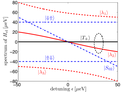
Figure 2: (color online). Spectrum of $H_{\mathrm{el}}$ in the relevant two-electron regime for $\Delta=40\mu\mathrm{eV}$ and $t=30\mu\mathrm{eV}$; shown here as a function of the interdot detuning parameter $\epsilon$. The three hybridized electronic eigenstates $\left|\lambda_{k}\right\rangle$ within the $S_{\mathrm{tot}}^{z}=0$ subspace are displayed in red, while the bare electronic states are shown in blue (dash-dotted lines). The homogeneous Zeeman splitting $\omega_{0}$ has been set to zero, so that the Pauli-blocked triplets $\left|T_{\pm}\right\rangle$ are degenerate. In this setting, the levels $\left|\lambda_{1,3}\right\rangle$ are far detuned from $\left|T_{\pm}\right\rangle$. Therefore, the spin-blockade is lifted pre-dominantly via the non-local electronic level $\left|\lambda_{2}\right\rangle$. The black dashed ellipse refers to a potential operational area of our scheme.

Electronic Hamiltonian.—In Eq.(19), $H_{\mathrm{el}}$ describes the electronic degrees of freedom of the DQD within the relevant two-electron subspace. It can be written as $\left(\hbar=1\right)$

$$H_{\mathrm{el}} = \omega_{0}\left(S_{L}^{z}+S_{R}^{z}\right)+\Delta\left(S_{R}^{z}-S_{L}^{z}\right)-\epsilon\left|S_{02}\right\rangle\left\langle S_{02}\right|$$ (20)

$$+t\left(\left|\Uparrow\Downarrow\right\rangle\left\langle S_{02}\right|-\left|\Downarrow\Uparrow\right\rangle\left\langle S_{02}\right|+\mathrm{h.c.}\right),$$

where the nuclear-polarization-dependent ’mean-field’ quantities $\bar{\omega}_{\mathrm{OH}}$ and $\Delta_{\mathrm{OH}}$ have been absorbed into the definitions of $\omega_{0}$ and $\Delta$ as $\omega_{0}=\omega_{\mathrm{ext}}+\bar{\omega}_{\mathrm{OH}}$ and $\Delta=\Delta_{\mathrm{ext}}+\Delta_{\mathrm{OH}}$, respectively. In previous theoretical work, this feedback of the Overhauser shift on the electronic energy levels has been identified as a means for controlling the nuclear spins via instabilities towards self-polarization; compare for example Ref.rudner07 . Apart from the OH contributions, $\omega_{\mathrm{ext}}$ and $\Delta_{\mathrm{ext}}$ denote the Zeeman splitting due to the homogeneous and inhomogeneous component of a potential external magnetic field, respectively. Furthermore, $\epsilon$ refers to the relative interdot energy detuning between the left and right dot. The interdot tunneling with coupling strength $t$ occurs exclusively in the singlet subspace due to Pauli spin-blockade. It is instructive to diagonalize the effective five-dimensional electronic Hamiltonian $H_{\mathrm{el}}$. The eigenstates of $H_{\mathrm{el}}$ within the $S_{\mathrm{tot}}^{z}=S_{L}^{z}+S_{R}^{z}=0$ subspace can be expressed as

$$\left|\lambda_{k}\right\rangle=\mu_{k}\left|\Uparrow\Downarrow\right\rangle+\nu_{k}\left|\Downarrow\Uparrow\right\rangle+\kappa_{k}\left|S_{02}\right\rangle,$$ (21)

for $k=1,2,3$ with corresponding eigenenergies $\epsilon_{k}$; compare Fig. 2.amplitudes Note that, throughout this work, the hybridized level $\left|\lambda_{2}\right\rangle$ plays a crucial role for the dynamics of the DQD system: Since the levels $\left|\lambda_{1,3}\right\rangle$ are energetically separated from all other electronic levels (for $t\gg\omega_{0},g_{\mathrm{hf}}$), $\left|\lambda_{2}\right\rangle$ represents the dominant channel for lifting of the Pauli-blockade; compare Fig. 2.

Electron transport.—After tracing out the reservoir degrees of freedom, electron transport induces dissipation in the electronic subspace: The Liouvillian

$$\mathcal{L}_{\Gamma}\rho=\sum_{k,\nu=\pm}\Gamma_{k}\mathcal{D}\left[\left|T_{\nu}\right\rangle\left\langle\lambda_{k}\right|\right]\rho,$$ (22)

with the short-hand notation for the Lindblad form $\mathcal{D}\left[c\right]\rho=c\rho c^{\dagger}-\frac{1}{2}\left\{c^{\dagger}c,\rho\right\}$, effectively models electron transport through the DQD; here, we have applied a rotating-wave approximation by neglecting terms rotating at a frequency of $\epsilon_{k}-\epsilon_{l}$ for $k\neq l$ (see Appendix B for details). Accordingly, the hybridized electronic levels $\left|\lambda_{k}\right\rangle\left(k=1,2,3\right)$ acquire a finite lifetime rudner11b and decay with a rate

$$\Gamma_{k}=\left|\left<\lambda_{k}|S_{02}\right>\right|^{2}\Gamma=\kappa_{k}^{2}\Gamma,$$ (23)

determined by their overlap with the localized singlet $\left|S_{02}\right\rangle$, back into the Pauli-blocked triplet subspace $\left\{\left|T_{\pm}\right\rangle\right\}$. Here, $\Gamma=\Gamma_{R}/2$, where $\Gamma_{R}$ is the sequential tunneling rate to the right lead.

Hyperfine interaction.—After splitting off the semiclassical quantities $\bar{\omega}_{\mathrm{OH}}$ and $\Delta_{\mathrm{OH}}$, the superoperator

$$\mathcal{V}\rho=-i\left[V_{\mathrm{HF}},\rho\right],$$ (24)

captures the remaining effects due to the HF coupling between electronic and nuclear spins. Within the eigenbasis of $H_{\mathrm{el}}$, the hyperfine flip-flop dynamics $H_{\mathrm{ff}}$, accounting for the exchange of excitations between the electronic and nuclear subsystem, takes on the form

$$H_{\mathrm{ff}}=\frac{a_{\mathrm{hf}}}{2}\sum_{k}\left[\left|\lambda_{k}\right\rangle\left\langle T_{+}\right|\otimes L_{k}+\left|\lambda_{k}\right\rangle\left\langle T_{-}\right|\otimes\mathbb{L}_{k}+\mathrm{h.c.}\right],$$ (25)

where the non-local nuclear jump operators

$$L_{k} = \nu_{k}A_{L}^{+}+\mu_{k}A_{R}^{+},$$ (26)

$$\mathbb{L}_{k} = \mu_{k}A_{L}^{-}+\nu_{k}A_{R}^{-},$$ (27)

are associated with lifting the spin-blockade from $\left|T_{+}\right\rangle$ and $\left|T_{-}\right\rangle$ via $\left|\lambda_{k}\right\rangle$, respectively. These operators characterize the effective coupling between the nuclear system and its electronic environment; they can be controlled externally via gate voltages as the parameters $t$ and $\epsilon$ define the amplitudes $\mu_{k}$ and $\nu_{k}$. Since generically $\mu_{k}\neq\nu_{k}$, the non-uniform electron spin density of the hybridized eigenstates $\left|\lambda_{k}\right\rangle$ introduces an asymmetry to flip a nuclear spin on the first or second dot.rudner11b

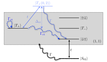
Figure 3: (color online). Scheme for the phenomenological cotunneling analysis. The spin-blocked triplet $\left|T_{+}\right\rangle$ is tunnel-coupled to the (virtually occupied) triplet $\left|T_{+}\left(0,2\right)\right\rangle$, localized on the right dot. Due to Pauli exclusion, this level is energetically well separated by the singlet-triplet splitting $\Delta_{\mathrm{st}}\gtrsim 400\mu\mathrm{eV}$. It has a finite lifetime $\Gamma^{-1}$ and may decay back (via a singly occupied level on the right dot) to $\left|T_{+}\right\rangle$ or via a series of fast coherent and incoherent intermediate processes end up in any level within the $(1,1)$ charge sector (shaded box), since $\left|S_{02}\right\rangle$ decays with a rate $\Gamma$ to all four $\left(1,1\right)$ states. The overall effectiveness of the process is set by the effective rate $\Gamma_{\mathrm{ct}}\approx\left(t/\Delta_{\mathrm{st}}\right)^{2}\Gamma$, depicted by dashed arrows.

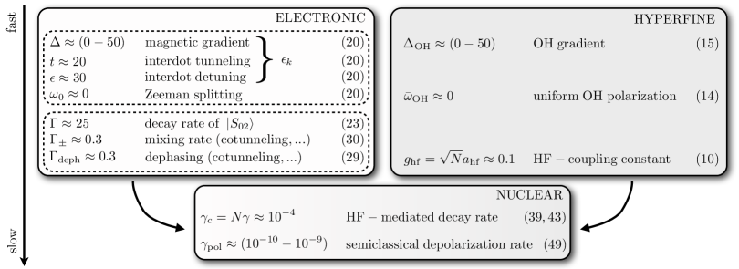
Figure 4: (color online). Schematic overview of the most important parameters in our model, grouped into electronic, hyperfine and HF-mediated nuclear quantities. Within the electronic quantities, we can differentiate between coherent and incoherent processes (compare dashed boxes). Typical numbers are given in $\mu\mathrm{eV}$, while the numbers in parentheses $(\cdot)$ refer to the corresponding equations in the text.

Electronic spin-blockade lifting.—Apart from the hyperfine mechanism described above, the Pauli blockade may also be lifted by other, purely electronic processes such as (i) cotunneling, (ii) spin-exchange with the leads, or (iii) spin-orbit coupling.rudner13 Although they do not exchange excitations with the nuclear spin bath, these processes have previously been shown to be essential to describe the nuclear spin dynamics in the Pauli blockade regime.rudner11b ; rudner07 ; qassemi09 In our analysis, it is crucial to include them as they affect the average electronic quasisteady state seen by the nuclei, while the exact, microscopic nature of the electronic decoherence processes does not play an important role for our proposal. Therefore, for concreteness, here we only describe exemplarily virtual tunneling processes via the doubly occupied triplet state labeled as $\left|T_{+}\left(0,2\right)\right\rangle$, while spin-exchange with the leads or spin-orbital effects are discussed in detail in Appendix D. Cotunneling via $\left|T_{-}\left(0,2\right)\right\rangle$ or $\left|T_{0}\left(0,2\right)\right\rangle$ can be analyzed along the same lines. As schematically depicted in Fig. 3, the triplet $\left|T_{+}\right\rangle$ with $\left(1,1\right)$ charge configuration is coherently coupled to $\left|T_{+}\left(0,2\right)\right\rangle$ by the interdot tunnel-coupling $t$. This transition is strongly detuned by the singlet-triplet splitting $\Delta_{\mathrm{st}}$. Once, the energetically high lying level $\left|T_{+}\left(0,2\right)\right\rangle$ is populated, it quickly decays with rate $\Gamma$ either back to $\left|T_{+}\right\rangle$ giving rise to a pure dephasing process within the low-energy subspace or to $\left\{\left|T_{-}\right\rangle,\left|\lambda_{k}\right\rangle\right\}$ via some fast intermediate steps, mediated by fast discharging and recharging of the DQD with the rate $\Gamma$.cotunneling-basis In our theoretical model (see below), the former is captured by the pure dephasing rate $\Gamma_{\mathrm{deph}}$, while the latter can be absorbed into the dissipative mixing rate $\Gamma_{\pm}$; compare Fig. 5 for a schematic illustration of $\Gamma_{\pm}$ and $\Gamma_{\mathrm{deph}}$, respectively. Since the singlet-triplet splitting is the largest energy scale in this process $\left(t,\Gamma\ll\Delta_{\mathrm{st}}\right)$, the effective rate for this virtual cotunneling mechanism can be estimated as

$$\Gamma_{\mathrm{ct}}\approx\left(t/\Delta_{\mathrm{st}}\right)^{2}\Gamma.$$ (28)

Equation (28) describes a virtually assisted process by which $t$ couples $\left|T_{+}\right\rangle$ to a virtual level, which can then escape via sequential tunneling $\sim\Gamma$; thus, it can be made relatively fast compared to typical nuclear timescales by working in a regime of efficient electron exchange with the leads $\sim\Gamma$.cotunneling-asymmetry For example, taking $t\approx 30\mu\mathrm{eV}$, $\Delta_{\mathrm{st}}\approx 400\mu\mathrm{eV}$ and $\Gamma\approx 50\mu\mathrm{eV}$, we estimate $\Gamma_{\mathrm{ct}}\approx 0.3\mu\mathrm{eV}$, which is fast compared to typical nuclear timescales. Note that, for more conventional, slower electronic parameters ($t\approx 5\mu\mathrm{eV}$, $\Gamma\approx 0.5\mu\mathrm{eV}$), indirect tunneling becomes negligibly small, $\Gamma_{\mathrm{ct}}\approx 5\times 10^{-5}\mu\mathrm{eV}\approx 5\times 10^{4}\mathrm{s}^{-1}$, in agreement with values given in Ref.rudner11b . Our analysis, however, is restricted to the regime, where indirect tunneling is fast compared to the nuclear dynamics; this regime of motional averaging has previously been shown to be beneficial for e.g. nuclear spin squeezing. rudner11a ; rudner07 Alternatively, spin-blockade may be lifted via spin-exchange with the leads. The corresponding rate $\Gamma_{\mathrm{se}}$ scales as $\Gamma_{\mathrm{se}}\sim\Gamma^{2}$, as compared to $\Gamma_{\mathrm{ct}}\sim t^{2}\Gamma$. Moreover, $\Gamma_{\mathrm{se}}$ depends strongly on the detuning of the $(1,1)$ levels from the Fermi levels of the leads. If this detuning is $\sim 500\mu\mathrm{eV}$ and for $\Gamma\approx 100\mu\mathrm{eV}$, we estimate $\Gamma_{\mathrm{se}}\approx 0.25\mu\mathrm{eV}$, which is commensurate with the desired motional averaging regime, whereas, for less efficient transport ($\Gamma\approx 1\mu\mathrm{eV}$) and stronger detuning $\sim 1\mathrm{meV}$, one obtains a negligibly small rate, $\Gamma_{\mathrm{se}}\approx 6\times 10^{-6}\mu\mathrm{eV}\approx 6\times 10^{3}\mathrm{s}^{-1}$. Again, this is in line with Ref.rudner11b . As discussed in more detail in Appendix D, these spin-exchange processes as well as spin-orbital effects can be treated on a similar footing as the interdot cotunneling processes discussed here. Therefore, to describe the net effect of various non-hyperfine mechanisms and to complete our theoretical description of electron transport in the spin-blockade regime, we add the following phenomenological Lindblad terms to our model

$$\mathcal{L}_{\mathrm{deph}}\rho = \frac{\Gamma_{\mathrm{deph}}}{2}\mathcal{D}\left[\left|T_{+}\right\rangle\left\langle T_{+}\right|-\left|T_{-}\right\rangle\left\langle T_{-}\right|\right]\rho,$$ (29)

$$\mathcal{L}_{\pm}\rho = \Gamma_{\pm}\sum_{\nu=\pm}\mathcal{D}\left[\left|T_{\bar{\nu}}\right\rangle\left\langle T_{\nu}\right|\right]\rho$$

$$+\Gamma_{\pm}\sum_{k,\nu}\mathcal{D}\left[\left|T_{\nu}\right\rangle\left\langle\lambda_{k}\right|\right]\rho+\mathcal{D}\left[\left|\lambda_{k}\right\rangle\left\langle T_{\nu}\right|\right]\rho.$$

Summary.—Before concluding the description of the system under study, let us quickly reiterate the ingredients of the master equation as stated in Eq.(1): It accounts for (i) the unitary dynamics within the DQD governed by $-i\left[H_{\mathrm{el}}+V_{\mathrm{HF}},\rho\right]$, (ii) electron-transport-mediated dissipation via $\mathcal{L}_{\Gamma}$ and (iii) dissipative mixing and dephasing processes described by $\mathcal{L}_{\pm}$ and $\mathcal{L}_{\mathrm{deph}}$, respectively. Finally, the most important parameters of our model are summarized in Fig. 4.

III Effective Nuclear Dynamics

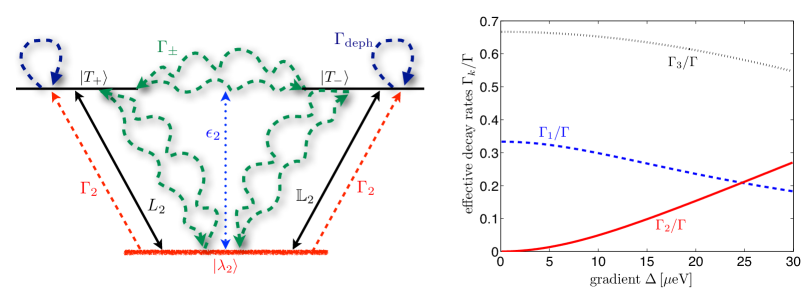
Figure 5: (color online). Left plot: Schematic illustration of coherent and incoherent processes within the effective three-level system $\left\{\left|T_{\pm}\right\rangle,\left|\lambda_{2}\right\rangle\right\}$: The level $\left|\lambda_{2}\right\rangle$ is detuned from $\left|T_{\pm}\right\rangle$ by $\epsilon_{2}$ and decays according to its overlap with the localized singlet with the rate $\Gamma_{2}=\kappa_{2}^{2}\Gamma$. Moreover, it is coherently coupled to the triplets $\left|T_{+}\right\rangle$ and $\left|T_{-}\right\rangle$ via the nonlocal nuclear operators $L_{2}$ and $\mathbb{L}_{2}$, respectively. Purely electronic spin-blockade lifting mechanisms such as cotunneling or spin-orbital effects result in effective dephasing and dissipative mixing rates, labeled as $\Gamma_{\mathrm{deph}}$ and $\Gamma_{\pm}$, respectively. The latter do not affect the nuclei directly, but lead to an unbiased population transfer within the electronic three-level system. In particular, mixing between $\left|T_{\pm}\right\rangle$ can arise from virtual occupation of $\left|\lambda_{1,3}\right\rangle$ or spin-orbit coupling. Right plot: Effective decay rates $\Gamma_{k}=\kappa_{k}^{2}\Gamma$, shown here for $\epsilon=t=30\mu\mathrm{eV}$. For small gradients, $\left|\lambda_{2}\right\rangle\approx\left|T_{0}\right\rangle$ and therefore it does not decay due to Pauli-blockade.

In this section we develop the general theoretical framework of our analysis which is built upon the fact that, generically, the nuclear spins evolve slowly on typical electronic timescales. Due to this separation of electronic and nuclear timescales, the system is subject to the slaving principle yamamoto99 implying that the electronic subsystem settles to a quasisteady state on a timescale much shorter than the nuclear dynamics. This allows us to adiabatically eliminate the electronic coordinates yielding an effective master equation on a coarse-grained timescale. Furthermore, the electronic quasisteady state is shown to depend on the state of the nuclei resulting in feedback mechanisms between the electronic and nuclear degrees of freedom. Specifically, here we analyze the dynamics of the nuclei coupled to the electronic three-level subspace spanned by the levels $\left|T_{\pm}\right\rangle$ and $\left|\lambda_{2}\right\rangle$. This simplification is justified for $t\gg\omega_{0},g_{\mathrm{hf}}$, since in this parameter regime the electronic levels $\left|\lambda_{1,3}\right\rangle$ are strongly detuned from the manifold $\left\{\left|T_{\pm}\right\rangle,\left|\lambda_{2}\right\rangle\right\}$; compare Fig. 2. Effects due to the presence of $\left|\lambda_{1,3}\right\rangle$ will be discussed separately in Secs. V and VI. Here, due to their fast decay with a rate $\Gamma_{1,3}$, they have already been eliminated adiabatically from the dynamics, leading to a dissipative mixing between the blocked triplet states $\left|T_{\pm}\right\rangle$ with rate $\Gamma_{\pm}$; alternatively, this mixing could come from spin-orbit coupling (see Appendix D for details). Moreover, for simplicity, we assume $\omega_{0}=0$ and neglect nuclear fluctuations arising from $H_{\mathrm{zz}}$. This approximation is in line with the semiclassical approach used below in order to study the nuclear polarization dynamics; for details we refer to Appendix F. In summary, all relevant coherent and incoherent processes within the effective three-level system $\left\{\left|T_{\pm}\right\rangle,\left|\lambda_{2}\right\rangle\right\}$ are schematically depicted in Fig. 5.

Intuitive picture.—The main results of this section can be understood from the fact that the level $\left|\lambda_{2}\right\rangle$ decays according to its overlap with the localized singlet, that is with a rate

$$\Gamma_{2}=\left|\left<\lambda_{2}|S_{02}\right>\right|^{2}\Gamma\overset{\Delta\rightarrow 0}{\longrightarrow}0$$ (31)

which in the low-gradient regime $\Delta\approx 0$ tends to zero, since then $\left|\lambda_{2}\right\rangle$ approaches the triplet $\left|T_{0}\right\rangle$ which is dark with respect to tunneling and therefore does not allow for electron transport; see Fig. 5. In other words, in the limit $\Delta\rightarrow 0$, the electronic level $\left|\lambda_{2}\right\rangle\rightarrow\left|T_{0}\right\rangle$ gets stabilized by Pauli-blockade. In this regime, we expect the nuclear spins to undergo some form of random diffusion process since the dynamics lack any directionality: the operators $L_{2}\left(\mathbb{L}_{2}\right)$ and their respective adjoints $L_{2}^{\dagger}(\mathbb{L}_{2}^{\dagger})$ act with equal strength on the nuclear system. In contrast, in the high-gradient regime, $\left|\lambda_{2}\right\rangle$ exhibits a significant singlet character and therefore gets depleted very quickly. Thus, $\left|\lambda_{2}\right\rangle$ can be eliminated adiabatically from the dynamics, the electronic subsystem settles to a maximally mixed state in the Pauli-blocked $\left|T_{\pm}\right\rangle$ subspace and the nuclear dynamics acquire a certain directionality in that now the nuclear spins experience dominantly the action of the non-local operators $L_{2}$ and $\mathbb{L}_{2}$, respectively. As will be shown below, this directionality features both the build-up of an Overhauser field gradient and entanglement generation between the two nuclear spin ensembles.

III.1 Adiabatic Elimination of Electronic Degrees of Freedom

Having separated the macroscopic semiclassical part of the nuclear Overhauser fields, the problem at hand features a hierarchy in the typical energy scales since the typical HF interaction strength is slow compared to all relevant electronic timescales. This allows for a perturbative approach to second order in $\mathcal{V}$ to derive an effective master equation for the nuclear subsystem.schuetz12 ; kessler12 To stress the perturbative treatment, the full quantum master equation can formally be decomposed as

$$\dot{\rho}=\left[\mathcal{L}_{0}+\mathcal{V}\right]\rho,$$ (32)

where the superoperator $\mathcal{L}_{0}$ acts on the electron degrees of freedom only and the HF interaction represents a perturbation. Thus, in zeroth order the electronic and nuclear dynamics are decoupled. In what follows, we will determine the effective nuclear evolution in the submanifold of the electronic quasisteady states of $\mathcal{L}_{0}$. The electronic Liouvillian $\mathcal{L}_{0}$ features a unique steady state sanchez13 , that is $\mathcal{L}_{0}\rho_{\mathrm{ss}}^{\mathrm{el}}=0$ for

$$\rho_{\mathrm{ss}}^{\mathrm{el}}=p\left(\left|T_{+}\right\rangle\left\langle T_{+}\right|+\left|T_{-}\right\rangle\left\langle T_{-}\right|\right)+\left(1-2p\right)\left|\lambda_{2}\right\rangle\left\langle\lambda_{2}\right|,$$ (33)

where

$$p=\frac{\Gamma_{\pm}+\Gamma_{2}}{3\Gamma_{\pm}+2\Gamma_{2}},$$ (34)

completely defines the electronic quasisteady state. It captures the competition between undirected population transfer within the the manifold $\left\{\left|T_{\pm}\right\rangle,\left|\lambda_{2}\right\rangle\right\}$ due to $\Gamma_{\pm}$ and a unidirectional, electron-transport-mediated decay of $\left|\lambda_{2}\right\rangle$. Moreover, it describes feedback between the electronic and nuclear degrees of freedom as the rate $\Gamma_{2}$ depends on the gradient $\Delta$ which incorporates the nuclear-polarization-dependent Overhauser gradient $\Delta_{\mathrm{OH}}$. We can immediately identify two important limits which will be analyzed in greater detail below: For $\Gamma_{\pm}\gg\Gamma_{2}$ we get $p=1/3$, whereas $\Gamma_{\pm}\ll\Gamma_{2}$ results in $p=1/2$, that is a maximally mixed state in the $\left|T_{\pm}\right\rangle$ subspace, since a fast decay rate $\Gamma_{2}$ leads to a complete depletion of $\left|\lambda_{2}\right\rangle$.

Since $\rho_{\mathrm{ss}}^{\mathrm{el}}$ is unique, the projector $\mathcal{P}$ on the subspace of zero eigenvalues of $\mathcal{L}_{0}$, i.e., the zeroth order steady states, is given by

$$\mathcal{P}\rho=\mathsf{Tr}_{\mathrm{el}}\left[\rho\right]\otimes\rho_{\mathrm{ss}}^{\mathrm{el}}=\sigma\otimes\rho_{\mathrm{ss}}^{\mathrm{el}}.$$ (35)

By definition, we have $\mathcal{P}\mathcal{L}_{0}=\mathcal{L}_{0}\mathcal{P}=0$ and $\mathcal{P}^{2}=\mathcal{P}$. The complement of $\mathcal{P}$ is $\mathcal{Q}=\mathbb{1}-\mathcal{P}$. Projection of the master equation on the $\mathcal{P}$ subspace gives in second-order perturbation theory

$$\frac{d}{dt}\mathcal{P}\rho=\left[\mathcal{P}\mathcal{V}\mathcal{P}-\mathcal{P}\mathcal{V}\mathcal{Q}\mathcal{L}_{0}^{-1}\mathcal{Q}\mathcal{V}\mathcal{P}\right]\rho,$$ (36)

from which we can deduce the required equation of motion $\dot{\sigma}=\mathcal{L}_{\mathrm{eff}}\left[\sigma\right]$ for the reduced density operator of the nuclear subsystem $\sigma=\mathsf{Tr}_{\mathrm{el}}\left[\mathcal{P}\rho\right]$ as

$$\dot{\sigma} = \mathsf{Tr}_{\mathrm{el}}\left[\mathcal{P}\mathcal{V}\mathcal{P}\rho-\mathcal{P}\mathcal{V}\mathcal{Q}\mathcal{L}_{0}^{-1}\mathcal{Q}\mathcal{V}\mathcal{P}\rho\right].$$ (37)

The subsequent, full calculation follows the general framework developed in Ref.kessler12b and is presented in detail in Appendices E and H. We then arrive at the following effective master equation for nuclear spins

$$\dot{\sigma} = \gamma\left\{p\left[\mathcal{D}\left[L_{2}\right]\sigma+\mathcal{D}\left[\mathbb{L}_{2}\right]\sigma\right]\right.$$

$$\left.+\left(1-2p\right)\left[\mathcal{D}\left[L_{2}^{\dagger}\right]+\mathcal{D}\left[\mathbb{L}_{2}^{\dagger}\right]\sigma\right]\right\}$$

$$+i\delta\left\{p\left(\left[L_{2}^{\dagger}L_{2},\sigma\right]+\left[\mathbb{L}_{2}^{\dagger}\mathbb{L}_{2},\sigma\right]\right)\right.$$

$$\left.-\left(1-2p\right)\left(\left[L_{2}L_{2}^{\dagger},\sigma\right]+\left[\mathbb{L}_{2}\mathbb{L}_{2}^{\dagger},\sigma\right]\right)\right\}.$$

Here, we have introduced the effective quantities

$$\gamma = \frac{a_{\mathrm{hf}}^{2}\tilde{\Gamma}}{2\left[\tilde{\Gamma}^{2}+\text{$\epsilon$}_{2}^{2}\right]},$$ (39)

$$\delta = \frac{a_{\mathrm{hf}}^{2}\epsilon_{2}}{4\left[\tilde{\Gamma}^{2}+\text{$\epsilon$}_{2}^{2}\right]},$$ (40)

and

$$\tilde{\Gamma}=\Gamma_{2}+2\Gamma_{\pm}+\frac{\Gamma_{\mathrm{deph}}}{4}.$$ (41)

The master equation in Eq.(III.1) is our first main result. It is of Lindblad form and incorporates electron-transport-mediated jump terms as well as Stark shifts. The two main features of Eq.(III.1) are: (i) The dissipative nuclear jump terms are governed by the nonlocal jump operators $L_{2}$ and $\mathbb{L}_{2}$, respectively. (ii) The effective dissipative rates $\sim p\gamma$ incorporate intrinsic electron-nuclear feedback effects as they depend on the macroscopic state of the nuclei via the parameter $p$ and the decay rate $\Gamma_{2}$. Because of this feedback mechanism, we can distinguish two very different fixed points for the coupled electron-nuclear evolution. This is discussed below.

III.2 Low-Gradient Regime: Random Nuclear Diffusion

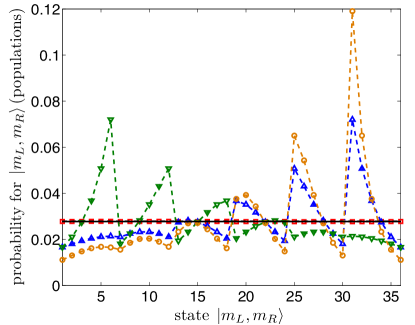
Figure 6: (color online). Exact steady-state as a function of the inhomogeneous splitting $\Delta$; results for $10$ nuclear spins, five in each quantum dot. We plot the diagonal elements of the nuclear steady-state density matrix $\sigma_{\mathrm{ss}}$ (i.e. the nuclear populations); its dimension is $\left(2J_{L}+1\right)\left(2J_{R}+1\right)=36$. For a small external gradient of the order of natural fluctuations of the Overhauser field (red squares) the nuclear system settles into the fully mixed state, as evidenced by the uniform populations of the nuclear levels. However, as we increase the gradient $\Delta$, the nuclear steady state starts to display a structure different from the fully mixed state, showing a dominant peak in the occupation of the nuclear level with maximum gradient, that is $\left|-J_{L},J_{R}\right\rangle$ and $\left|J_{L},-J_{R}\right\rangle$ for $\Delta>0$ and $\Delta<0$, respectively. The upward triangles, downward triangles and circles refer to $\Delta=5\mu\mathrm{eV}$, $\Delta=-5\mu\mathrm{eV}$ and $\Delta=10\mu\mathrm{eV}$, respectively. Other numerical parameters are: $\Gamma=10\mu\mathrm{eV}$, $\Gamma_{\pm}=0.3\mu\mathrm{eV}$, $\Gamma_{\mathrm{deph}}=3\mu\mathrm{eV}$, $\omega_{0}=0$, $t=\mathrm{20}\mu\mathrm{eV}$ and $\epsilon=30\mu\mathrm{eV}$.

As argued qualitatively above, in the low-gradient regime where $\left|\lambda_{2}\right\rangle\approx\left|T_{0}\right\rangle$, the nuclear master equation given in Eq.(III.1) lacks any directionality. Accordingly, the resulting dynamics may be viewed as a random nuclear diffusion process. Indeed, in the limit $\Gamma_{2}\rightarrow 0$, it is easy to check that $p=1/3$ and $\sigma_{\mathrm{ss}}\propto\mathbb{1}$ is a steady-state solution. Therefore, both the electronic and the nuclear subsystem settle into the fully mixed state with no preferred direction nor any peculiar polarization characteristics.

This analytical argument is corroborated by exact numerical simulations (i.e., without having eliminated the electronic degrees of freedom) for the full five-level electronic system coupled to ten $(N_{L}=N_{R}=5)$ nuclear spins. Here, we assume homogeneous HF coupling (effects due to non-uniform HF couplings are discussed in Section VII): Then, the total spins $J_{i}$ are conserved and it is convenient to describe the nuclear spin system in terms of Dicke states $\left|J_{i},m_{i}\right\rangle$ with total spin quantum number $J_{i}$ and spin projection $m_{i}=-J_{i},\dots,J_{i}$. Fixing the (conserved) total spin quantum numbers $J_{i}=N_{i}/2$, we write in short $\left|J_{L},m_{L}\right\rangle\otimes\left|J_{R},m_{R}\right\rangle=\left|m_{L},m_{R}\right\rangle$. In order to realistically mimic the perturbative treatment of the HF coupling in an experimentally relevant situation where $N\approx 10^{6}$, here the HF coupling constant $g_{\mathrm{hf}}=A_{\mathrm{HF}}/\sqrt{N}$ is scaled down to a constant value of $g_{\mathrm{hf}}=0.1\mu\mathrm{eV}$. Moreover, let us for the moment neglect the nuclear fluctuations due to $H_{\mathrm{zz}}$, in order to restrict the following analysis to the semiclassical part of the nuclear dynamics; compare also previous theoretical studies.rudner07 ; rudner11b ; vink09 In later setions, this part of the dynamics will be taken into account again. In particular, we compute the steady state and analyze its dependence on the gradient $\Delta$: Experimentally, $\Delta$ could be induced intrinsically via a nuclear Overhauser gradient $\Delta_{\mathrm{OH}}$ or extrinsically via a nano- or micro-magnet.petersen13 ; pioro-ladriere08 The results are displayed in Fig. 6: Indeed, in the low-gradient regime the nuclear subsystem settles into the fully mixed state. However, outside of the low-gradient regime, the nuclear subsystem is clearly driven away from the fully mixed state and shows a tendency towards the build-up of a nuclear Overhauser gradient. For $\Delta>0$, we find numerically an increasing population (in descending order) of the levels $\left|-J_{L},J_{R}\right\rangle,\left|-J_{L}+1,J_{R}-1\right\rangle$ etc., whereas for $\Delta<0$ strong weights are found at $\left|J_{L},-J_{R}\right\rangle,\left|J_{L}-1,-J_{R}+1\right\rangle,\dots$ which effectively increases $\Delta$ such that the nuclear spins actually tend to self-polarize. This trend towards self-polarization and the peculiar structure of the nuclear steady state $\sigma_{\mathrm{ss}}$ displayed in Fig. 6 is in very good agreement with the ideal nuclear two-mode squeezedlike steady-state that we are to construct analytically in the next subsection.

III.3 High-Gradient Regime: Entanglement Generation

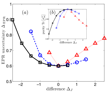
Figure 7: (color online). EPR-uncertainty $\Delta_{\mathrm{EPR}}$ and purity of the (exact) nuclear dark states fulfilling $\mathcal{D}\left[L_{2}\right]\sigma_{\mathrm{ss}}+\mathcal{D}\left[\mathbb{L}_{2}\right]\sigma_{\mathrm{ss}}=0$ for small system sizes $J_{i}$.simiplification-delta=00003D0 We fix $J_{L}$ to $J_{L}=1$ (triangles), $J_{L}=2$ (circles) and $J_{L}=3$ (squares) and compute $\sigma_{\mathrm{ss}}$ for different values of $\Delta_{J}$; $J_{R}$ runs from $0.5$ up to $3.5$. In the symmetric scenario $\Delta_{J}=0$, $\sigma_{\mathrm{ss}}$ is pure and given by the two-mode squeezed like state $\sigma_{\mathrm{ss}}=\left|\xi_{\mathrm{ss}}\right\rangle\left\langle\xi_{\mathrm{ss}}\right|$. For $\Delta_{J}\neq 0$, $\sigma_{\mathrm{ss}}$ is mixed; however, the purity $\mathsf{Tr}\left[\sigma_{\mathrm{ss}}^{2}\right]$ (inset) as well as $\Delta_{\mathrm{EPR}}$ increase with the system size $J_{L}+J_{R}$. In all cases, $\sigma_{\mathrm{ss}}$ was found to be unique. Here, we have set $\left|\xi\right|=0.25$.

In the high-gradient regime the electronic level $\left|\lambda_{2}\right\rangle$ overlaps significantly with the localized singlet $\left|S_{02}\right\rangle$. For $\Gamma_{2}\gg\Gamma_{\pm}$ it decays sufficiently fast such that it can be eliminated adiabatically from the dynamics. As can be seen from Eqs.(33) and (34), on typical nuclear timescales, the electronic subsystem then quickly settles into the quasisteady state given by $\rho_{\mathrm{ss}}^{\mathrm{el}}=\left(\left|T_{+}\right\rangle\left\langle T_{+}\right|+\left|T_{-}\right\rangle\left\langle T_{-}\right|\right)/2$ and the effective master equation for the nuclear spin density matrix $\sigma$ simplifies to

$$\dot{\sigma}=\frac{\gamma}{2}\left[\mathcal{D}\left[L_{2}\right]\sigma+\mathcal{D}\left[\mathbb{L}_{2}\right]\sigma\right]+i\frac{\delta}{2}\left(\left[L_{2}^{\dagger}L_{2},\sigma\right]+\left[\mathbb{L}_{2}^{\dagger}\mathbb{L}_{2},\sigma\right]\right).$$ (42)

For later reference, the typical timescale of this dissipative dynamics is set by the rate

$$\gamma_{c}=N\gamma=\frac{g_{\mathrm{hf}}^{2}\tilde{\Gamma}}{2\left[\tilde{\Gamma}^{2}+\text{$\epsilon$}_{2}^{2}\right]},$$ (43)

which is collectively enhanced by a factor of $N\approx 10^{6}$ to account for the norm of the collective nuclear spin operators $A_{i}^{\pm}$. This results in the typical HF-mediated interaction strength of $g_{\mathrm{hf}}=\sqrt{N}a_{\mathrm{hf}}$,schuetz12 and for typical parameter values we estimate $\gamma_{c}\approx 10^{-4}\mu\mathrm{eV}$.

This evolution gives rise to the desired, entangling nuclear squeezing dynamics: It is easy to check that all pure stationary solutions $\left|\xi_{\mathrm{ss}}\right\rangle$ of this Lindblad evolution can be found via the dark-state condition $L_{2}\left|\xi_{\mathrm{ss}}\right\rangle=\mathbb{L}_{2}\left|\xi_{\mathrm{ss}}\right\rangle=0$. Next, we explicitly construct $\left|\xi_{\mathrm{ss}}\right\rangle$ in the limit of equal dot sizes $\left(N_{L}=N_{R}\right)$ and uniform HF coupling $\left(a_{i,j}=N/N_{i}\right)$, and generalize our results later. In this regime, again it is convenient to describe the nuclear system in terms of Dicke states $\left|J_{i},k_{i}\right\rangle$, where $k_{i}=0,\dots,2J_{i}$. For the symmetric scenario $J_{L}=J_{R}=J$, one can readily verify that the dark state condition is satisfied by the (unnormalized) pure state

$$\left|\xi_{\mathrm{ss}}\right\rangle=\sum_{k=0}^{2J}\xi^{k}\left|J,k\right\rangle_{L}\otimes\left|J,2J-k\right\rangle_{R}.$$ (44)

This nuclear state may be viewed as an extension of the two-mode squeezed state familiar from quantum optics muschik11 to finite dimensional Hilbert spaces. The parameter $\xi=-\nu_{2}/\mu_{2}$ quantifies the entanglement and polarization of the nuclear system. Note that unlike in the bosonic case (discussed in detail in Section V), the modulus of $\xi$ is unconfined. Both $\left|\xi\right|<1$ and $\left|\xi\right|>1$ are allowed and correspond to states of large positive (negative) OH field gradients, respectively, and the system is invariant under the corresponding symmetry transformation ($\mu_{2}\leftrightarrow\nu_{2}$, $A_{L,R}^{z}\rightarrow-A_{L,R}^{z}$). As we discuss in detail in Section IV, this symmetry gives rise to a bistability in the steady state, as for every solution with positive OH field gradient ($\Delta_{\mathrm{OH}}>0$), we find a second one with negative gradient ($\Delta_{\mathrm{OH}}<0$). As a first indication for this bistability, also compare the green and blue curve in Fig. 6: For $\Delta\gg 0$, the dominant weight of the nuclear steady state is found in the level $\left|-J_{L},J_{R}\right\rangle$, that is the Dicke state with maximum positive Overhauser gradient, whereas for $\Delta\ll 0$, the weight of the nuclear stationary state is peaked symmetrically at $\left|J_{L},-J_{R}\right\rangle$, corresponding to the Dicke state with maximum negative Overhauser gradient.

In the asymmetric scenario $J_{L}\neq J_{R}$, one can readily show that a pure dark-state solution does not exist. Thus, we resort to exact numerical solutions for small system sizes $J_{i}\approx 3$ to compute the nuclear steady state-solution $\sigma_{\mathrm{ss}}$. To verify the creation of steady-state entanglement between the two nuclear spin ensembles, we take the EPR uncertainty as a figure of merit. It is defined via

$$\Delta_{\mathrm{EPR}}=\frac{\mathrm{var}\left(I_{L}^{x}+I_{R}^{x}\right)+\mathrm{var}\left(I_{L}^{y}+I_{R}^{y}\right)}{\left|\left\langle I_{L}^{z}\right\rangle\right|+\left|\left\langle I_{R}^{z}\right\rangle\right|},$$ (45)

and measures the degree of nonlocal correlations. For an arbitrary state, $\Delta_{\mathrm{EPR}}<1$ implies the existence of such non-local correlations, whereas $\Delta_{\mathrm{EPR}}\geq 1$ for separable states.muschik11 The results are displayed in Fig. 7. First of all, the numerical solutions confirm the analytical result in the symmetric limit where the asymmetry parameter $\Delta_{J}=J_{R}-J_{L}$ is zero. In the asymmetric setting, where $J_{L}\neq J_{R}$, the steady state $\sigma_{\mathrm{ss}}$ is indeed found to be mixed, that is $\mathsf{Tr}\left[\sigma_{\mathrm{ss}}^{2}\right]<1$. However, both the amount of generated entanglement as well as the purity of $\sigma_{\mathrm{ss}}$ tend to increase, as we increase the system size $J_{L}+J_{R}$ for a fixed value of $\Delta_{J}$. For fixed $J_{i}$, we have also numerically verified that the steady-state solution is unique.

In practical experimental situations one deals with a mixture of different $J_{i}$ subspaces. The width of the nuclear spin distribution is typically $\Delta_{J}\sim\sqrt{N}$, but may even be narrowed further actively; see for example Refs.rudner07 ; vink09 . The numerical results displayed above suggest that the amount of entanglement and purity of the nuclear steady state increases for smaller absolute values of the relative asymmetry $\Delta_{J}/J=\left(J_{R}-J_{L}\right)/\left(J_{L}+J_{R}\right)$. In Fig. 7, $\Delta_{\mathrm{EPR}}<1$ is still observed even for $\left|\Delta_{J}\right|/J=2.5/3.5\approx 0.7$. Thus, experimentally one might still obtain entanglement in a mixture of different large $J_{i}$ subspaces for which the relative width is comparatively small, $\Delta_{J}/J\approx\sqrt{N}/N\approx 10^{-3}\ll 1$. Intuitively, the idea is that for every pair $\left\{J_{L},J_{R}\right\}$ with $J_{L}\approx J_{R}$ the system is driven towards a state similar to the ideal two-mode squeezedlike state given in Eq.(44). This will also be discussed in more detail in Section V.

IV Dynamic Nuclear Polarization

In the previous section we have identified a low-gradient regime, where the nuclear spins settle into a fully mixed state, and a high-gradient regime, where the ideal nuclear steady state was found to be a highly polarized, entangled two-mode squeezedlike state. Now, we provide a thorough analysis which reveals the multi-stability of the nuclear subsystem and determines the connection between these two very different regimes. It is shown that, beyond a critical polarization, the nuclear spin system becomes self-polarizing and is driven towards a highly polarized OH gradient.

To this end, we analyze the nuclear spin evolution within a semiclassical approximation which neglects coherences among different nuclei. This approach has been well studied in the context of central spin systems (see for example Ref.gullans10 and references therein) and is appropriate on timescales longer than nuclear dephasing times.christ07 This approximation will be justified self-consistently. The analysis is based on the effective QME given in Eq.(III.1). First, assuming homogeneous HF coupling and equal dot sizes $\left(N_{L}=N_{R}=N\right)$, we construct dynamical equations for the expectation values of the collective nuclear spins $\left\langle I_{i}^{z}\right\rangle_{t}$, $i=L,R$, where $I_{i}^{\nu}=\sum_{j}\sigma_{i,j}^{\nu}$ for $\nu=\pm,z$. To close the corresponding differential equations we use a semiclassical factorization scheme resulting in two equations of motion for the two nuclear dynamical variables $\left\langle I_{L}^{z}\right\rangle_{t}$ and $\left\langle I_{R}^{z}\right\rangle_{t}$, respectively. This extends previous works on spin dynamics in double quantum dots, where a single dynamical variable for the nuclear polarization was used to explain the feedback mechanism in this system; see for example Refs.rudner07 ; lopez-moniz11 . The corresponding nonlinear differential equations are then shown to yield nonlinear equations for the equilibrium polarizations. Generically, the nuclear polarization is found to be multi-stable (compare also Refs.rudner11b ; danon09b ) and, depending on the system’s parameters, we find up to three stable steady state solutions for the OH gradient $\Delta_{\mathrm{OH}}^{\mathrm{ss}}$, two of which are highly polarized in opposite directions and one is unpolarized; compare Fig. 8 for a schematic illustration.

At this point, some short remarks are in order: First, the analytical results obtained within the semiclassical approach are confirmed by exact numerical results for small sets of nuclei; see Appendix G. Second, by virtue of the semiclassical decoupling scheme used here, our results can be generalized to the case of inhomogeneous HF coupling in a straightforward way with the conclusions remaining essentially unchanged. Third, for simplicity here we assume the symmetric scenario of vanishing external fields $\omega_{\mathrm{ext}}=\Delta_{\mathrm{ext}}=0$; therefore, $\Delta=\Delta_{\mathrm{OH}}$. However, as shown in Section VII and Appendix G one may generalize our results to finite external fields: This opens up another experimental knob to tune the desired steady-state properties of the nuclei.

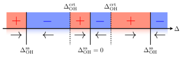
Figure 8: (color online). Schematic representation of the multistability of the nuclear dynamics. For initial nuclear gradients smaller than $\Delta_{\mathrm{OH}}^{\mathrm{crt}}$ the nuclear system is attracted towards the trivial zero-polarization solution ($\Delta_{\mathrm{OH}}^{\mathrm{ss}}=0$). Upon surpassing $\Delta_{\mathrm{OH}}^{\mathrm{crt}}$, however, the system enters into an electron-nuclear feedback loop and the nuclear dynamics turn self-polarizing such that large OH gradients can be reached in the steady state. This is schematically denoted by $\pm$ referring to the sign of $\dot{\Delta}_{I^{z}}$ which determines the stable fixed point the nuclear system is attracted to in the steady state (see arrows).

Intuitive picture.—Before going through the calculation, let us sketch an intuitive picture that can explain the instability of the nuclear spins towards self-polarization and the corresponding build-up of a macroscopic nuclear OH gradient: In the high-gradient regime, the nuclear spins predominantly experience the action of the nonlocal jump operators $L_{2}=\nu_{2}A_{L}^{+}+\mu_{2}A_{R}^{+}$ and $\mathbb{L}_{2}=\mu_{2}A_{L}^{-}+\nu_{2}A_{R}^{-}$, respectively, both of them acting with the same rate $\gamma$ on the nuclear spin ensembles. For example, for $\Delta>0$ and $\epsilon>0$, where $\mu_{2}>\nu_{2}$, the first nuclear ensemble gets exposed more strongly to the action of the collective lowering operator $A_{L}^{-}$, whereas the second ensemble preferentially experiences the action of the raising operator $A_{R}^{+}$; therefore, the two nuclear ensembles are driven towards polarizations of opposite sign. The second steady solution featuring a large OH gradient with opposite sign is found along the same lines for $\mu_{2}<\nu_{2}$. Therefore, our scheme provides a good dynamic nuclear polarization (DNP) protocol for $\mu_{2}\gg\nu_{2}$ $\left(\left|\xi\right|\ll 1\right)$, or vice-versa for $\mu_{2}\ll\nu_{2}$ $\left(\left|\xi\right|\gg 1\right)$.

Semiclassical analysis.—Using the usual angular momentum commutation relations $\left[I^{z},I^{\pm}\right]=\pm I^{\pm}$ and $\left[I^{+},I^{-}\right]=2I^{z}$, Eq.(III.1) readily yields two rate equations for the nuclear polarizations $\left\langle I_{i}^{z}\right\rangle_{t}$, $i=L,R$. We then employ a semiclassical approach by neglecting correlations among different nuclear spins, that is

$$\left\langle\sigma_{i}^{+}\sigma_{j}^{-}\right\rangle=\begin{cases}0&,i\neq j\\ \left\langle\sigma_{i}^{z}\right\rangle+\frac{1}{2}&,i=j\end{cases}$$ (46)

which allows us to close the equations of motion for the nuclear polarizations $\left\langle I_{i}^{z}\right\rangle$. This leads to the two following nonlinear equations of motion,

$$\frac{d}{dt}\left\langle I_{L}^{z}\right\rangle_{t} = -\gamma_{\mathrm{pol}}\left[\left\langle I_{L}^{z}\right\rangle_{t}+\frac{N}{2}\frac{\chi}{\gamma_{\mathrm{pol}}}\right],$$ (47)

$$\frac{d}{dt}\left\langle I_{R}^{z}\right\rangle_{t} = -\gamma_{\mathrm{pol}}\left[\left\langle I_{R}^{z}\right\rangle_{t}-\frac{N}{2}\frac{\chi}{\gamma_{\mathrm{pol}}}\right],$$ (48)

where we have introduced the effective HF-mediated depolarization rate $\gamma_{\mathrm{pol}}$ and pumping rate $\chi$ as

$$\gamma_{\mathrm{pol}} = \gamma\left(\mu_{2}^{2}+\nu_{2}^{2}\right)\left(1-p\right),$$ (49)

$$\chi = \gamma\left(\mu_{2}^{2}-\nu_{2}^{2}\right)\left(3p-1\right),$$ (50)

with the rate $\gamma$ given in Eq.(39). Clearly, Eqs.(47) and (48) already suggest that the two nuclear ensembles are driven towards opposite polarizations. The nonlinearity is due to the fact that both $\chi$ and $\gamma_{\mathrm{pol}}$ depend on the gradient $\Delta$ which itself depends on the nuclear polarizations $\left\langle I_{i}^{z}\right\rangle_{t}$; at this stage of the anlysis, however, $\Delta$ simply enters as a parameter of the underlying effective Hamiltonian. Equivalently, the macroscopic dynamical evolution of the nuclear system may be expressed in terms of the total net polarization $P\left(t\right)=\left\langle I_{L}^{z}\right\rangle_{t}+\left\langle I_{R}^{z}\right\rangle_{t}$ and the polarization gradient $\Delta_{I^{z}}=\left\langle I_{R}^{z}\right\rangle_{t}-\left\langle I_{L}^{z}\right\rangle_{t}$ as

$$\dot{P}\left(t\right) = -\gamma_{\mathrm{pol}}P\left(t\right),$$ (51)

$$\frac{d}{dt}\Delta_{I^{z}} = -\gamma_{\mathrm{pol}}\left[\Delta_{I^{z}}-N\frac{\chi}{\gamma_{\mathrm{pol}}}\right].$$ (52)

Fixed-point analysis.—In what follows, we examine the fixed points of the semiclassical equations derived above. First of all, since $\gamma_{\mathrm{pol}}>0\,\forall P,\Delta_{I^{z}}$, Eq.(51) simply predicts that in our system no homogeneous nuclear net polarization $P$ will be produced. In contrast, any potential initial net polarization is exponentially damped to zero in the long-time limit, since in the steady state $\lim_{t\rightarrow\infty}P\left(t\right)=0$. This finding is in agreement with previous theoretical results showing that, due to angular momentum conservation, a net nuclear polarization cannot be pumped in a system where the HF-mediated relaxation rate for the blocked triplet levels $\left|T_{+}\right\rangle$ and $\left|T_{-}\right\rangle$, respectively, is the same; see, e.g., Ref.rudner07 and references therein.

The dynamical equation for $\Delta_{I^{z}}$, however, is more involved: The effective rates $\gamma_{\mathrm{pol}}=\gamma_{\mathrm{pol}}\left(\Delta\right)$ and $\chi=\chi\left(\Delta\right)$ in Eq.(52) depend on the nuclear-polarization dependent parameter $\Delta$. This nonlinearity opens up the possibility for multiple steady-state solutions. From Eqs.(47) and (48) we can immediately identify the fixed points $\left\langle I_{i}^{z}\right\rangle_{\mathrm{ss}}$ of the nuclear polarization dynamics as $\pm\left(N/2\right)\chi/\gamma_{\mathrm{pol}}$. Consequently, the two nuclear ensembles tend to be polarized along opposite directions, that is $\left\langle I_{L}^{z}\right\rangle_{\mathrm{ss}}=-\left\langle I_{R}^{z}\right\rangle_{\mathrm{ss}}$. The corresponding steady-state nuclear polarization gradient $\Delta_{I^{z}}^{\mathrm{ss}}$, scaled in terms of its maximum value $N$, is given by

$$\frac{\Delta_{I^{z}}^{\mathrm{ss}}}{N}=\mathcal{R}\left(\Delta\right)=\Lambda\frac{3p-1}{1-p}.$$ (53)

Here, we have introduced the nonlinear function $\mathcal{R}\left(\Delta\right)$ which depends on the purely electronic quantity

$$\Lambda=\Lambda\left(\Delta\right)=\frac{\mu_{2}^{2}-\nu_{2}^{2}}{\mu_{2}^{2}+\nu_{2}^{2}}=\frac{1-\xi^{2}}{1+\xi^{2}}.$$ (54)

According to Eq.(53), the function $\mathcal{R}\left(\Delta\right)$ determines the nuclear steady-state polarization. While the functional dependence of $\Lambda$ on the gradient $\Delta$ can give rise to two highly polarized steady-state solutions with opposite nuclear spin polarization, for $\left|\mu_{2}\right|\gg\left|\nu_{2}\right|$ and $\left|\mu_{2}\right|\ll\left|\nu_{2}\right|$, respectively, the second factor in Eq.(53) may prevent the system from reaching these highly polarized fixed points. Based on Eq.(53), we can identify the two important limits discussed previously: For $\Gamma_{2}\ll\Gamma_{\pm}$, the electronic subsystem settles into the steady-state solution $p=1/3$ and the nuclear system is unpolarized, as the second factor in Eq.(53) vanishes. This is what we identified above as the nuclear diffusion regime in which the nuclear subsystem settles into the unpolarized fully mixed state. In the opposite limit, where $\Gamma_{2}\gg\Gamma_{\pm}$, the electronic subsystem settles into $p\approx 1/2$. In this limit, the second factor in Eq.(53) becomes $1$ and the functional dependence of $\Lambda\left(\Delta\right)$ dominates the behavior of $\mathcal{R}\left(\Delta\right)$ such that large nuclear OH gradients can be achieved in the steady state. The electron-nuclear feedback loop can then be closed self-consistently via $\Delta_{\mathrm{OH}}^{\mathrm{ss}}/\Delta_{\mathrm{OH}}^{\mathrm{max}}=\mathcal{R}\left(\Delta_{\mathrm{OH}}^{\mathrm{ss}}\right),$ where, in analogy to Eq.(53), $\Delta_{\mathrm{OH}}^{\mathrm{ss}}$ has been scaled in units of its maximum value $\Delta_{\mathrm{OH}}^{\mathrm{max}}=A_{\mathrm{HF}}/2$. Points fulfilling this condition can be found at intersections of $\mathcal{R}\left(\Delta\right)$ with $\Delta_{\mathrm{OH}}^{\mathrm{ss}}/\Delta_{\mathrm{OH}}^{\mathrm{max}}$ . This is elaborated below.

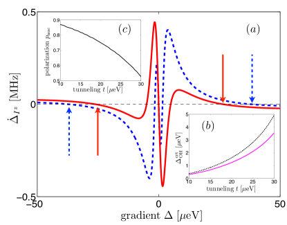
Figure 9: (color online). Semiclassical solution to the nuclear polarization dynamics: tristability of the nuclear steady state. (a) Instantaneous nuclear polarization rate $\dot{\Delta}_{I^{z}}$ for $t=20\mu\mathrm{eV}$ (dashed) and $t=30\mu\mathrm{eV}$ (solid), respectively. Stable fixed points are found at $\dot{\Delta}_{I^{z}}=0$ and $d\dot{\Delta}_{I^{z}}/d\Delta<0$. The nuclear system is driven towards one of the highly polarized fixed points (indicated by arrows), if the initial gradient $\Delta$ exceeds a critical threshold $\left|\Delta_{\mathrm{OH}}^{\mathrm{crt}}\right|$, shown in (b) for $\Gamma_{\pm}=0.1\mu\mathrm{eV}$ (dashed) and $\Gamma_{\pm}=0.05\mu\mathrm{eV}$ (solid), respectively. (c) By tuning $t$, one can achieve $\left|\xi\right|\ll 1$ leading to a nuclear polarization of $\lesssim 90\%$. Other numerical parameters in $\mu\mathrm{eV}$: $\Gamma=25$, $\epsilon=30$, $\Gamma_{\pm}=0.1$ (except for the solid line in (b) where $\Gamma_{\pm}=0.05$) and $\Gamma_{\mathrm{deph}}=0.1$.

To gain further insights into the nuclear polarization dynamics, we evaluate $\dot{\Delta}_{I^{z}}$ as given in Eq.(52). The results are displayed in Fig. 9. Stable fixed points of the dynamics are determined by $\dot{\Delta}_{I^{z}}=0$ and $d\dot{\Delta}_{I^{z}}/d\Delta<0$ as opposed to unstable fixed points where $d\dot{\Delta}_{I^{z}}/d\Delta>0$. In this way it is ensured that fluctuations of $\Delta_{I^{z}}$ away from a stable fixed point are corrected by a restoring intrinsic pump effect.vink09 ; danon09b ; bluhm10b We can identify parameter regimes in which the nuclear system features three stable fixed points. As schematically depicted in Fig. 8, they are interspersed by two unstable points referred to as $\Delta_{\mathrm{OH}}^{\mathrm{crt}}$. Therefore, in general, the nuclear steady-state polarization is found to be tri-stable: Two of the stable fixed points are high-polarization solutions of opposite sign, supporting a macroscopic OH gradient, while one is the trivial zero-polarization solution. The unstable points $\Delta_{\mathrm{OH}}^{\mathrm{crt}}$ represent critical values for the initial OH gradient marking the boundaries of a critical region. If the initial gradient lies outside of this critical region, the OH gradient runs into one of the highly polarized steady states. Otherwise, the nuclear system gets stuck in the zero-polarization steady state. Note that $\Delta_{\mathrm{OH}}^{\mathrm{crt}}$ is tunable: To surpass the critical region one needs $\Gamma_{2}\gg\Gamma_{\pm}$; thus, the critical region can be destabilized by making $\Gamma_{\pm}$ smaller [compare Fig. 9(b)] which is lower bounded by $\Gamma_{\pm}\gg\gamma_{c}$ in order to justify the elimination of the electronic degrees of freedom. For typical parameters we thus estimate $\Delta_{\mathrm{OH}}^{\mathrm{crt}}\approx(3-5)\mu\mathrm{eV}$ which sets the required initial $\Delta$ in order to kick-start the nuclear self-polarization process. Experimentally, this could be realized either via an initial nuclear polarization of $p_{\mathrm{nuc}}\approx(5-10)\%$ or an on-chip nanomagnet.petersen13 ; pioro-ladriere08

Timescales.—In order to reach a highly polarized steady state, approximately $\sim 10^{5}$ nuclear spin flips are required. We estimate $\dot{\Delta}_{I^{z}}\approx 0.1\mathrm{MHz}$ and, thus, the total time for the polarization process is therefore approximately $\sim 10^{5}/0.1\mathrm{MHz}\approx 1\mathrm{s}$. This order of magnitude estimate is in very good agreement with typical timescales observed in nuclear polarization experiments.takahashi11 Moreover, $\gamma_{\mathrm{pol}}^{-1}\approx 1\mathrm{s}$ is compatible with our semiclassical approach, since nuclear spins typically dephase at a rate of $\sim\mathrm{kHz}$.takahashi11 ; gullans10 Finally, in any experimental situation, the nuclear spins are subject to relaxation and diffusion processes which prohibit complete polarization of the nuclear spins. Therefore, in order to capture other depolarizing processes that go beyond our current analysis, one could add an additional phenomenological nuclear depolarization rate $\gamma_{\mathrm{dp}}$ by simply making the replacement $\gamma_{\mathrm{pol}}\left(\Delta\right)\rightarrow\gamma_{\mathrm{pol}}\left(\Delta\right)+\gamma_{\mathrm{dp}}$. Since typically $\gamma_{\mathrm{dp}}^{-1}\approx 15\mathrm{s}$,danon09b however, these additional processes are slow in comparison to the intrinsic rate $\gamma_{\mathrm{pol}}$ and should not lead to any qualitative changes of our results.

V Steady-State Entanglement Generation

In Section III we have identified a high-gradient regime which—after adiabatically eliminating all electronic coordinates—supports a rather simple description of the nuclear dynamics on a coarse-grained timescale. Now, we extend our previous analysis and provide a detailed analysis of the nuclear dynamics in the high-gradient regime. In particular, this includes perturbative effects due to the presence of the so far neglected levels $\left|\lambda_{1,3}\right\rangle$. To this end, we apply a self-consistent Holstein-Primakoff approximation, which reexpresses nuclear fluctuations around the semiclassical state in terms of bosonic modes. This enables us to approximately solve the nuclear dynamics analytically, to directly relate the ideal nuclear steady state to a two-mode squeezed state familiar from quantum optics and to efficiently compute several entanglement measures.

V.1 Extended Nuclear Master Equation in the High-Gradient Regime

In the high-gradient regime the electronic system settles to a quasisteady state $\rho_{\mathrm{ss}}^{\mathrm{el}}=\rho_{\mathrm{target}}^{\mathrm{el}}=\left(\left|T_{+}\right\rangle\left\langle T_{+}\right|+\left|T_{-}\right\rangle\left\langle T_{-}\right|\right)/2$ [compare Eqs.(33) and (34)] on a timescale short compared to the nuclear dynamics; deviations due to (small) populations of the hybridized levels are discussed in Appendix J. We then follow the general adiabatic elimination procedure discussed in Section III to obtain an effective master equation for the nuclear spins in the submanifold of the electronic quasisteady state $\rho_{\mathrm{target}}^{\mathrm{el}}$. The full calculation is presented in detail in Appendix H. In summary, the generalized effective master equation reads

$$\dot{\sigma} = \sum_{k}\left[\frac{\gamma_{k}^{+}}{2}\mathcal{D}\left[L_{k}\right]\sigma+\frac{\gamma_{k}^{-}}{2}\mathcal{D}\left[\mathbb{L}_{k}\right]\sigma\right]+i\left[H_{\mathrm{Stark}},\sigma\right]$$ (55)

$$+\gamma_{\mathrm{zz}}\sum_{i,j}\left[\delta A_{i}^{z}\sigma\delta A_{j}^{z}-\frac{1}{2}\left\{\delta A_{j}^{z}\delta A_{i}^{z},\sigma\right\}\right].$$

Here, we have introduced the effective HF-mediated decay rates

$$\gamma_{k}^{+} = \frac{a_{\mathrm{hf}}^{2}\tilde{\Gamma}_{k}}{2\left[\Delta_{k}^{2}+\tilde{\Gamma}_{k}^{2}\right]},$$ (56)

$$\gamma_{k}^{-} = \frac{a_{\mathrm{hf}}^{2}\tilde{\Gamma}_{k}}{2\left[\delta_{k}^{2}+\tilde{\Gamma}_{k}^{2}\right]},$$ (57)

where $\tilde{\Gamma}_{k}=\Gamma_{k}+3\Gamma_{\pm}+\Gamma_{\mathrm{deph}}/4$ and the detuning parameters

$$\Delta_{k} = \epsilon_{k}-\omega_{0},$$ (58)

$$\delta_{k} = \epsilon_{k}+\omega_{0},$$ (59)

specify the splitting between the electronic eigenstate $\left|\lambda_{k}\right\rangle$ and the Pauli-blocked triplet states $\left|T_{+}\right\rangle$ and $\left|T_{-}\right\rangle$, respectively. The effective nuclear Hamiltonian

$$H_{\mathrm{Stark}}=\sum_{k}\frac{\Delta_{k}^{+}}{2}L_{k}^{\dagger}L_{k}+\frac{\Delta_{k}^{-}}{2}\mathbb{L}_{k}^{\dagger}\mathbb{L}_{k}$$ (60)

is given in terms of the second-order Stark shifts

$$\Delta_{k}^{+} = \frac{a_{\mathrm{hf}}^{2}\Delta_{k}}{4\left[\Delta_{k}^{2}+\tilde{\Gamma}_{k}^{2}\right]},$$ (61)

$$\Delta_{k}^{-} = \frac{a_{\mathrm{hf}}^{2}\delta_{k}}{4\left[\delta_{k}^{2}+\tilde{\Gamma}_{k}^{2}\right]}.$$ (62)

Lastly, in Eq.(55) we have set $\gamma_{\mathrm{zz}}=a_{\mathrm{hf}}^{2}/(5\Gamma_{\pm})$. For $\omega_{0}=0$, we have $\gamma_{k}^{+}=\gamma_{k}^{-}$ and $\Delta_{k}^{+}=\Delta_{k}^{-}$. When disregarding effects due to $H_{\mathrm{zz}}$ and neglecting the levels $\left|\lambda_{1,3}\right\rangle$, i.e., only keeping $k=2$ in Eq.(55), indeed, we recover the result of the Section III; see Eq.(42). As shown in Appendix I, the nuclear HF-mediated jump terms in Eq.(55) can be brought into diagonal form which features a clear hierarchy due to the predominant coupling to $\left|\lambda_{2}\right\rangle$. To stress this hierarchy in the effective nuclear dynamics $\dot{\sigma}=\mathcal{L}_{\mathrm{eff}}\sigma$, we write

$$\dot{\sigma}=\mathcal{L}_{\mathrm{id}}\sigma+\mathcal{L}_{\mathrm{nid}}\sigma,$$ (63)

where the first term captures the dominant coupling to the electronic level $\left|\lambda_{2}\right\rangle$ only and is given as

$$\mathcal{L}_{\mathrm{id}}\sigma = \frac{\gamma_{2}^{+}}{2}\mathcal{D}\left[L_{2}\right]\sigma+\frac{\gamma_{2}^{-}}{2}\mathcal{D}\left[\mathbb{L}_{2}\right]\sigma$$ (64)

$$+i\frac{\Delta_{2}^{+}}{2}\left[L_{2}^{\dagger}L_{2},\sigma\right]+i\frac{\Delta_{2}^{-}}{2}\left[\mathbb{L}_{2}^{\dagger}\mathbb{L}_{2},\sigma\right],$$

whereas the remaining non-ideal part $\mathcal{L}_{\mathrm{nid}}$ captures all remaining effects due to the coupling to the far-detuned levels $\left|\lambda_{1,3}\right\rangle$ and the OH fluctuations described by $H_{\mathrm{zz}}$.

V.2 Holstein-Primakoff Approximation and Bosonic Formalism

To obtain further insights into the nuclear spin dynamics in the high-gradient regime, we now restrict ourselves to uniform hyperfine coupling $\left(a_{i,j}=N/N_{i}\right)$ and apply a Holstein-Primakoff (HP) transformation to the collective nuclear spin operators $I_{i}^{\alpha}=\sum_{j}\sigma_{i,j}^{\alpha}$ for $\alpha=\pm,z$; generalizations to non-uniform coupling will be discussed separately below in Section VII. This treatment of the nuclear spins has proven valuable already in previous theoretical studies.kessler12 In the present case, it allows for a detailed study of the nuclear dynamics including perturbative effects arising from $\mathcal{L}_{\mathrm{nid}}$.

The (exact) Holstein-Primakoff (HP) transformation expresses the truncation of the collective nuclear spin operators to a total spin $J_{i}$ subspace in terms of a bosonic mode.kessler12 Note that for uniform HF coupling the total nuclear spin quantum numbers $J_{i}$ are conserved quantities. Here, we consider two nuclear spin ensembles that are polarized in opposite directions of the quantization axis $\hat{z}$. Then, the HP transformation can explicitly be written as

$$I_{L}^{-} = \sqrt{2J_{L}}\sqrt{1-\frac{b_{L}^{\dagger}b_{L}}{2J_{L}}}b_{L},$$ (65)

$$I_{L}^{z} = b_{L}^{\dagger}b_{L}-J_{L},$$

for the first ensemble, and similarly for the second ensemble

$$I_{R}^{+} = \sqrt{2J_{R}}\sqrt{1-\frac{b_{R}^{\dagger}b_{R}}{2J_{R}}}b_{R},$$ (66)

$$I_{R}^{z} = J_{R}-b_{R}^{\dagger}b_{R}.$$

Here, $b_{i}$ denotes the annihilation operator of the bosonic mode $i=L,R$. Next, we expand the operators of Eqs.(65) and (66) in orders of $\varepsilon_{i}=1/\sqrt{J_{i}}$ which can be identified as a perturbative parameter.kessler12 This expansion can be justified self-consistently provided that the occupation numbers of the bosonic modes $b_{i}$ are small compared to $2J_{i}$. Thus, here we consider the subspace with large collective spin quantum numbers, that is $J_{i}\sim\mathcal{O}\left(N/2\right)$. Accordingly, up to second order in $\varepsilon_{L}\approx\varepsilon_{R}$, the hyperfine Hamiltonian can be rewritten as

$$H_{\mathrm{HF}}=H_{\mathrm{sc}}+H_{\mathrm{ff}}+H_{\mathrm{zz}},$$ (67)

where the semiclassical part $H_{\mathrm{sc}}$ reads

$$H_{\mathrm{sc}} = a_{R}J_{R}S_{R}^{z}-a_{L}J_{L}S_{L}^{z}$$ (68)

$$= \text{$\bar{\omega}$}_{\mathrm{OH}}\left(S_{L}^{z}+S_{R}^{z}\right)+\Delta_{\mathrm{OH}}\left(S_{R}^{z}-S_{L}^{z}\right).$$ (69)

Here, we have introduced the individual HF coupling constants $a_{i}=A_{\mathrm{HF}}/N_{i}$ and

$$\text{$\bar{\omega}$}_{\mathrm{OH}} = \Delta_{\mathrm{OH}}^{\mathrm{max}}\left(\mathrm{p}_{R}-\mathrm{p}_{L}\right)/2,$$ (70)

$$\text{$\bar{\Delta}$}_{\mathrm{OH}} = \Delta_{\mathrm{OH}}^{\mathrm{max}}\left(\mathrm{p}_{L}+\mathrm{p}_{R}\right)/2,$$ (71)

with $\mathrm{p}_{i}=J_{i}/J_{i}^{\mathrm{max}}=2J_{i}/N_{i}$ denoting the degree of polarization in dot $i=L,R$ and $\Delta_{\mathrm{OH}}^{\mathrm{max}}=A_{\mathrm{HF}}/2\approx 50\mu\mathrm{eV}$. Within the HP approximation, the hyperfine dynamics read

$$H_{\mathrm{ff}}=\frac{a_{L}}{2}\sqrt{2J_{L}}S_{L}^{+}b_{L}+\frac{a_{R}}{2}\sqrt{2J_{R}}S_{R}^{+}b_{R}^{\dagger}+\mathrm{h.c.},$$ (72)

and

$$H_{\mathrm{zz}}=a_{L}S_{L}^{z}b_{L}^{\dagger}b_{L}-a_{R}S_{R}^{z}b_{R}^{\dagger}b_{R}.$$ (73)

Note that, due to the different polarizations in the two dots, the collective nuclear operators $I_{i}^{+}$ map onto bosonic annihilation (creation) operators in the left (right) dot, respectively. The expansion given above implies a clear hierarchy in the Liouvillian $\mathcal{L}_{0}+\mathcal{V}$ allowing for a perturbative treatment of the leading orders and adiabatic elimination of the electron degrees of freedom whose evolution is governed by the fastest timescale of the problem: while the semiclassical part $H_{\mathrm{sc}}/J_{i}\sim\mathcal{O}\left(1\right)$, the HF interaction terms scales as $H_{\mathrm{ff}}/J_{i}\sim\mathcal{O}\left(\varepsilon\right)$ and $H_{\mathrm{zz}}/J_{i}\sim\mathcal{O}\left(\varepsilon^{2}\right)$; also compare Ref.kessler12 . To make connection with the analysis of the previous subsection, we give the following explicit mapping

$$A_{L}^{+} \approx \eta_{L}b_{L}^{\dagger},\qquad\delta A_{L}^{z}=\zeta_{L}b_{L}^{\dagger}b_{L},$$ (74)

$$A_{R}^{+} \approx \eta_{R}b_{R},\qquad\delta A_{R}^{z}=-\zeta_{R}b_{R}^{\dagger}b_{R}.$$

Here, the parameters $\zeta_{i}=N/N_{i}$ and $\eta_{i}=\zeta_{i}\sqrt{2J_{i}}$ capture imperfections due to either different dot sizes $\left(N_{L}\neq N_{R}\right)$ and/or different total spin manifolds $\left(J_{L}\neq J_{R}\right)$. Moreover, within the HP treatment $\mathcal{V}$ can be split up into a first $\left(\mathcal{L}_{\mathrm{ff}}\right)$ and a second-order effect $\left(\mathcal{L}_{\mathrm{zz}}\right)$; therefore, in second-order perturbation theory, the effective nuclear dynamics simplify to [compare Eq.(37)]

$$\dot{\sigma}=\mathsf{Tr}_{\mathrm{el}}\left[\mathcal{P}\mathcal{L}_{\mathrm{ff}}\mathcal{P}\rho+\mathcal{P}\mathcal{L}_{\mathrm{zz}}\mathcal{P}\rho-\mathcal{P}\mathcal{L}_{\mathrm{ff}}\mathcal{Q}\mathcal{L}_{0}^{-1}\mathcal{Q}\mathcal{L}_{\mathrm{ff}}\mathcal{P}\rho\right],$$ (75)

since higher-order effects due to $\mathcal{L}_{\mathrm{zz}}$ can be neglected self-consistently to second order.

Ideal nuclear target state.—Within the HP approximation and for the symmetric setting $\eta_{1}=\eta_{2}=\eta$, the dominant nuclear jump operators $L_{2}$ and $\mathbb{L}_{2}$, describing the lifting of the spin blockade via the electronic level $\left|\lambda_{2}\right\rangle$, can be expressed in terms of nonlocal bosonic modes as

$$L_{2} = \eta\sqrt{\mu_{2}^{2}-\nu_{2}^{2}}a,$$ (76)

$$\mathbb{L}_{2} = \eta\sqrt{\mu_{2}^{2}-\nu_{2}^{2}}\tilde{a},$$ (77)

where $a=\nu b_{L}^{\dagger}+\mu b_{R}$ and $\tilde{a}=\mu b_{L}+\nu b_{R}^{\dagger}$. Here, $\mu=\mu_{2}/\sqrt{\mu_{2}^{2}-\nu_{2}^{2}}$ and $\nu=\nu_{2}/\sqrt{\mu_{2}^{2}-\nu_{2}^{2}}$, such that $\mu^{2}-\nu^{2}=1$. Therefore, due to $\left[a,a^{\dagger}\right]=1=\left[\tilde{a},\tilde{a}^{\dagger}\right]$ and $\left[a,\tilde{a}^{\dagger}\right]=0=\left[a,\tilde{a}\right]$, the operators $a$ and $\tilde{a}$ refer to two independent, properly normalized nonlocal bosonic modes. In this picture, the (unique) ideal nuclear steady state belonging to the dissipative evolution $\mathcal{L}_{\mathrm{id}}\sigma$ in Eq.(64) is well known to be a two-mode squeezed state

$$\left|\Psi_{\mathrm{TMS}}\right\rangle=\mu^{-1}\sum_{n}\xi^{n}\left|n\right\rangle_{L}\otimes\left|n\right\rangle_{R}$$ (78)

with $\xi=-\nu/\mu$:muschik11 $\left|\Psi_{\mathrm{TMS}}\right\rangle$ is the common vacuum of the non-local bosonic modes $a$ and $\tilde{a}$, $a\left|\Psi_{\mathrm{TMS}}\right\rangle=\tilde{a}\left|\Psi_{\mathrm{TMS}}\right\rangle=0$. It features entanglement between the number of excitations $n$ in the first and second dot. Going back to collective nuclear spins, this translates to perfect correlations between the degree of polarization in the two nuclear ensembles. Note that $\left|\Psi_{\mathrm{TMS}}\right\rangle$ represents the dark state $\left|\xi_{\mathrm{ss}}\right\rangle$ given in Eq.(44) in the zeroth-order HP limit where the truncation of the collective spins to $J_{i}$ subspaces becomes irrelevant.

Bosonic steady-state solution.—Within the HP approximation, the nuclear dynamics generated by the full effective Liouvillian $\dot{\sigma}=\mathcal{L}_{\mathrm{eff}}\sigma$ are quadratic in the bosonic creation $b_{i}^{\dagger}$ and annihilation operators $b_{i}$. Therefore, the nuclear dynamics are purely Gaussian and an exact solution is feasible. Based on Eq.(55) and Eq.(74), one readily derives a closed dynamical equation for the second-order moments

$$\frac{d}{dt}\boldsymbol{\gamma}=\mathcal{M}\boldsymbol{\gamma}+\boldsymbol{C},$$ (79)

where $\boldsymbol{\gamma}$ is a vector comprising the second-order moments, that is $\boldsymbol{\gamma}=\left(\left\langle b_{i}^{\dagger}b_{j}\right\rangle_{t},\left\langle b_{i}^{\dagger}b_{j}^{\dagger}\right\rangle_{t},\dots\right)^{\top}$ and $\boldsymbol{C}$ is a constant vector. The solution to Eq.(79) is given by

$$\boldsymbol{\gamma}\left(t\right)=e^{\mathcal{M}t}\boldsymbol{c}_{0}-\mathcal{M}^{-1}\boldsymbol{C},$$ (80)

where $\boldsymbol{c}_{0}$ is an integration constant. Accordingly, provided that the dynamics generated by $\mathcal{M}$ is contractive (see section VI for more details), the steady-state solution is found to be

$$\boldsymbol{\gamma}_{\mathrm{ss}}=-\mathcal{M}^{-1}\boldsymbol{C}.$$ (81)

Based on $\boldsymbol{\gamma}_{\mathrm{ss}}$, one can construct the steady-state covariance matrix (CM), defined as $\Gamma_{ij}^{\mathrm{CM}}=\left\langle\left\{R_{i},R_{j}\right\}\right\rangle-2\left\langle R_{i}\right\rangle\left\langle R_{j}\right\rangle,$ where $\left\{R_{i},i=1,\dots,4\right\}=\left\{X_{L},P_{L},X_{R},P_{R}\right\}$; here, $X_{i}=(b_{i}+b_{i}^{\dagger})/\sqrt{2}$ and $P_{i}=i(b_{i}^{\dagger}-b_{i})/\sqrt{2}$ refer to the quadrature operators related to the bosonic modes $b_{i}$. By definition, Gaussian states are fully characterized by the first and second moments of the field operators $R_{i}$. Here, the first order moments can be shown to vanish. The entries of the CM are real numbers: since they constitute the variances and covariances of quantum operators, they can be detected experimentally via nuclear spin variance and correlation measurements.laurat05

We now turn to the central question of whether the steady-state entanglement inherent to the ideal target state $\left|\Psi_{\mathrm{TMS}}\right\rangle$ is still present in the presence of the undesired terms described by $\mathcal{L}_{\mathrm{nid}}$. In our setting, this is conveniently done via the CM, which encodes all information about the entanglement properties:schwager10 It allows us to compute certain entanglement measures efficiently in order to make qualitative and quantitative statements about the degree of entanglement.schwager10 Here, we will consider the following quantities: For symmetric states, the entanglement of formation $E_{F}$ can be computed easily.giedke03 ; wolf04 It measures the minimum number of singlets required to prepare the state through local operations and classical communication. For symmetric states, this quantification of entanglement is fully equivalent to the one provided by the logarithmic negativity $E_{\mathcal{N}}$; the latter is determined by the smallest symplectic eigenvalues of the CM of the partially transposed density matrix.vidal02 Lastly, in the HP picture the EPR uncertainty defined in Eq.(45) translates to $\Delta_{\mathrm{EPR}}=\left[\mathrm{var}\left(X_{L}+X_{R}\right)+\mathrm{var}\left(P_{L}-P_{R}\right)\right]/2$. For the ideal target state $\left|\Psi_{\mathrm{TMS}}\right\rangle$, we find $\Delta_{\mathrm{EPR}}^{\mathrm{id}}=\left(\mu-\nu\right)^{2}=\left(1-\left|\xi\right|\right)/\left(1+\left|\xi\right|\right)<1$. Finally, one can also compute the fidelity $\mathcal{F}\left(\sigma_{\mathrm{ss}},\sigma_{\mathrm{target}}\right)$ which measures the overlap between the steady state generated by the full dynamics $\dot{\sigma}=\mathcal{L}_{\mathrm{eff}}\sigma$ and the ideal target state $\sigma_{\mathrm{target}}=\left|\Psi_{\mathrm{TMS}}\right\rangle\left\langle\Psi_{\mathrm{TMS}}\right|$. schwager10

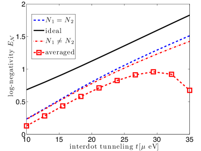
Figure 10: (color online). Steady-state entanglement generation between the two nuclear spin ensembles. $E_{\mathcal{N}}>0$ indicates the creation of entanglement. The black solid curve refers to the idealized, symmetric setting where the undesired HF-coupling to $\left|\lambda_{1,3}\right>$ has been ignored and where $J_{L}=J_{R}=\mathrm{p}J_{\mathrm{max}}$; here, the nuclear polarization $\mathrm{p}=0.8$ and $N_{L}=N_{R}=2J_{\mathrm{max}}=10^{6}$. The blue-dashed line then also takes into account coupling to $\left|\lambda_{1,3}\right>$, while the red (dash-dotted) curve in addition accounts for an asymmetric dot size: $N_{R}=0.8N_{L}=8\times 10^{5}$. Additionally, classical uncertainty (red squares) in the total spin $J_{i}$ quantum numbers leads to a reduced amount of entanglement, but does not disrupt it completely; here, we have set the range of the (uniform) distribution to $\Delta_{J_{i}}=50\sqrt{N_{i}}$. Other numerical parameters: $\omega_{0}=0$, $\Gamma=25\mu\mathrm{eV}$, $\epsilon=30\mu\mathrm{eV}$, $3\Gamma_{\pm}+\Gamma_{\mathrm{deph}}/4=0.5\mu\mathrm{eV}$.

As illustrated in Fig. 10, the generation of steady-state entanglement persists even in presence of the undesired noise terms described by $\mathcal{L}_{\mathrm{nid}}$, asymmetric dot sizes $\left(N_{L}\neq N_{R}\right)$ and classical uncertainty in total spins $J_{i}$: The maximum amount of entanglement that we find (in the symmetric scenario $N_{L}=N_{R}$) is approximately $E_{\mathcal{N}}\approx 1.5$, corresponding to an entanglement of formation $E_{F}\approx(1-2)\mathrm{ebit}$ and an EPR uncertainty of $\Delta_{\mathrm{EPR}}\approx 0.4$. When tuning the interdot tunneling parameter from $t=10\mu\mathrm{eV}$ to $t=35\mu\mathrm{eV}$, the squeezing parameter $\left|\xi\right|=\left|\nu_{2}/\mu_{2}\right|$ increases from $\sim 0.2$ to $\sim 0.6$, respectively; this is because (for fixed $\Delta,\epsilon>0$) and increasing $t$, $\epsilon_{2}$ approaches 0 and the relative weight of $\nu_{2}$ as compared to $\mu_{2}$ increases. Ideally, this implies stronger squeezing of the steady state of $\mathcal{L}_{\mathrm{id}}$ and therefore a greater amount of entanglement (compare the solid line in Fig. 10), but, at the same time, it renders the target state more susceptible to undesired noise terms. Stronger squeezing leads to a larger occupation of the bosonic HP modes (pictorially, the nuclear target state leaks farther into the Dicke ladder) and eventually to a break-down of the approximative HP description. The associated critical behavior in the nuclear spin dynamics can be understood in terms of a dynamical phase transition kessler12 , which will be analyzed in greater detail in the next section.

VI Criticality

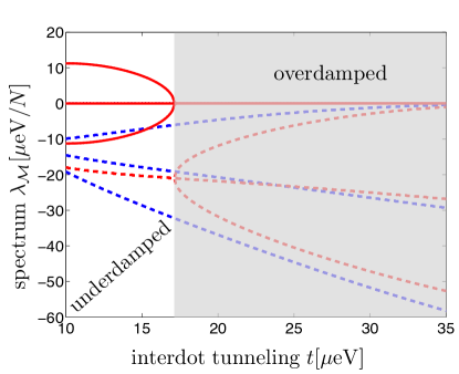
Figure 11: (color online). Spectrum of $\mathcal{M}$. Real (dashed) and imaginary parts (solid) for $\Gamma=25\mu\mathrm{eV}$ (blue) and $\Gamma=50\mu\mathrm{eV}$ (red). A dynamical phase transition is found at the bifurcation separating an underdamped from an overdamped region (see gray shading for the spectrum displayed in red). The critical point $t_{\mathrm{crt}}\approx 37\mu\mathrm{eV}$ is reached where the smallest decay rate $\left(\mathrm{ADR}\right)$ becomes zero. Other numerical parameters as those for the dashed curve in Fig. 10.

Based on the Holstein-Primakoff analysis outlined above, we now show that the nuclear spin dynamics exhibit a dynamical quantum phase transition which originates from the competition between dissipative terms and unitary dynamics. This rather generic phenomenon in open quantum systems results in nonanalytic behaviour in the spectrum of the nuclear spin Liouvillian, as is well known from the paradigm example of the Dicke model.kessler12 ; nagy11 ; dimer07 ; diehl10

The nuclear dynamics in the vicinity of the stationary state are described by the stability matrix $\mathcal{M}$. Resulting from a systematic expansion in the system size, the (complex) eigenvalues of $\mathcal{M}$ correspond exactly to the low-excitation spectrum of the full system Liouvillian given in Eq.(1) in the thermodynamic limit ($J\rightarrow\infty$). A non-analytic change of steady state properties (indicating a steady state phase transition) can only occur if the spectral gap of $\mathcal{M}$ closes.kessler12 ; hoening12 The relevant gap in this context is determined by the eigenvalue with the largest real part different from zero [from here on referred to as the asymptotic decay rate (ADR)]. The ADR determines the rate by which the steady state is approached in the long time limit.

As depicted in Fig. 11, the system reaches such a critical point at $t_{\mathrm{crt}}\approx 37\mu\mathrm{eV}$ where the ADR (red/blue dotted lines closest to zero) becomes zero. At this point, the dynamics generated by $\mathcal{M}$ become non-contractive [compare Eq.(80)] and the nuclear fluctuations diverge, violating the self-consistency condition of low occupation numbers in the bosonic modes $b_{i}$ and thus leading to a break-down of the HP approximation. Consequently, the dynamics cannot furhter be described by the dynamical matrix $\mathcal{M}$ indicating a qualitative change in the system properties and a steady state phase transition.

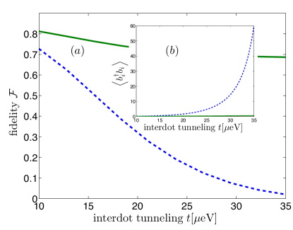
Figure 12: (color online). (a) Fidelity $\mathcal{F}$ of the nuclear steady-state with the two-mode squeezed target state. The blue-dashed line accounts for the full nuclear Liouvillian $\mathcal{L}_{\mathrm{eff}}$ for the symmetric setting $\left(N_{L}=N_{R}\right)$, while the green solid line refers to the same setting in the absence of any Stark-shift terms. Therefore, the decreasing fidelity $\mathcal{F}$ (blue dashed line) and a diverging number of HP bosons shown in (b) is due to undesired Stark shift terms included in $\mathcal{L}_{\mathrm{eff}}$. Here, $\eta_{L}=\eta_{R}$ and therefore $\left\langle b_{L}^{\dagger}b_{L}\right\rangle=\left\langle b_{R}^{\dagger}b_{R}\right\rangle$; asymmetric settings where $\eta_{L}\neq\eta_{R}$ entail small asymmetries in the number of HP bosons. For other numerical parameters compare the dashed curve in Fig. 10.

To obtain further insights into the cross-over of the maximum real part of the eigenvalues $\lambda_{\mathcal{M}}$ of the matrix $\mathcal{M}$ from negative to positive values, we analyze the effect of the nuclear Stark shift terms [Eq.(60)] in more detail. In the HP regime, up to irrelevant constant terms, the Stark shift Hamiltonian $H_{\mathrm{Stark}}$ can be written as

$$H_{\mathrm{Stark}}=\epsilon_{L}^{\mathrm{st}}b_{L}^{\dagger}b_{L}+\epsilon_{R}^{\mathrm{st}}b_{R}^{\dagger}b_{R}+\epsilon_{LR}^{\mathrm{st}}\left[b_{L}b_{R}+b_{L}^{\dagger}b_{R}^{\dagger}\right],$$ (82)

The relevant parameters $\epsilon_{\nu}^{\mathrm{st}}$ introduced above are readily obtained from Eqs.(60) and (74). In the symmetric setting $\eta_{L}=\eta_{R}$, it is instructive to re-express $H_{\mathrm{Stark}}$ in terms of the squeezed, non-local bosonic modes $a=\nu b_{L}^{\dagger}+\text{$\mu$}b_{R}$ and $\tilde{a}=\mu b_{L}+\nu b_{R}^{\dagger}$ [see Eqs. (76) and (77)] whose common vacuum is the ideal steady state of $\mathcal{L}_{\mathrm{id}}$. Up to an irrelevant constant term, $H_{\mathrm{Stark}}$ takes on the form

$$H_{\mathrm{Stark}}=\Delta_{a}a^{\dagger}a+\Delta_{\tilde{a}}\tilde{a}^{\dagger}\tilde{a}+g_{a\tilde{a}}\left(a\tilde{a}+a^{\dagger}\tilde{a}^{\dagger}\right).$$ (83)

With respect to the entanglement dynamics, the first two terms do not play a role as the ideal steady state $\left|\Psi_{\mathrm{TMS}}\right\rangle$ is an eigenstate thereof. However, the last term is an active squeezing term in the non-local bosonic modes: It does not preserve the excitation number in the modes $a,\tilde{a}$ and may therefore drive the nuclear system away from the vacuum by pumping excitations into the system. Numerically, we find that the relative strength of $g_{a\tilde{a}}$ increases compared to the desired entangling dissipative terms when tuning the interdot tunneling parameter $t$ towards $t_{\mathrm{crt}}$. We therefore are confronted with two competing effects while tuning the interdot coupling $t$. On the one hand, the dissipative dynamics tries to pump the system into the vacuum of the modes $a$ and $\tilde{a}$ [see Eqs. (76) and (77)], which become increasingly squeezed as we increase $t$. On the other hand, an increase in $t$ leads to enhanced coherent dynamics (originating from the nuclear Stark shift $H_{\mathrm{Stark}}$) which try to pump excitations in the system [Eq.(83)]. This competition between dissipative and coherent dynamics is known to be at the origin of many dissipative phase transitions, and has been extensively studied, e.g., in the context of the Dicke phase transition.dimer07 ; nagy11

As shown in Fig. 12, the observed critical behaviour in the nuclear spin dynamics can indeed be traced back to the presence of the nuclear Stark shift terms $H_{\mathrm{Stark}}$: here, when tuning the system towards the critical point $t_{\mathrm{crt}}$, the diverging number of HP bosons is shown to be associated with the presence of $H_{\mathrm{Stark}}$. Moreover, for relatively low values of the squeezing parameter $\left|\xi\right|$, we obtain a relatively high fidelity $\mathcal{F}$ with the ideal two-mode squeezed state, close to 80%. For stronger squeezing, however, the target state becomes more susceptible to the undesired noise terms, first leading to a reduction of $\mathcal{F}$ and eventually to a break-down of the HP approximation.

Aside from this phase transition in the steady state, we find nonanalyticities at non-zero values of the nuclear ADR, indicating a change in the dynamical properties of the system which cannot be detected in steady-state observables.kessler12 Rather, the system displays anomalous behaviour approaching the stationary state: As shown Fig. 11, we can distinguish two dynamical phases,alvarez06 ; danieli07 ; eleuch14 ; lesanovsky13 an underdamped and an overdamped one, respectively. The splitting of the real parts of $\mathcal{M}$ coincides with vanishing imaginary parts. Thus, in the overdamped regime, perturbing the system away from its steady state leads to an exponential, non-oscillating return to the stationary state. A similar underdamped region in direct vicinity of the phase transition can be found in the dissipative Dicke phase transition.dimer07 ; nagy11

VII Implementation

This Section is devoted to the experimental realization of our proposal. First, we summarize the experimental requirements of our scheme. Thereafter, we address several effects that are typically encountered in realistic systems, but which have been neglected so far in our analysis. This includes non-uniform HF coupling, larger individual nuclear spins $\left(I>1/2\right)$, external magnetic fields, different nuclear species, internal nuclear dynamics and charge noise.

Experimental requirements.—Our proposal relies on the predominant spin-blockade lifting via the electronic level $\left|\lambda_{2}\right\rangle$ and the adiabatic elimination of the electronic degrees of freedom: First, the condition $t\gg\omega_{0},g_{\mathrm{hf}}$ ascertains a predominant lifting of the Pauli-blockade via the hybridized, nonlocal level $\left|\lambda_{2}\right\rangle$. To reach the regime in which the electronic subsystem settles into the desired quasisteady state $\rho_{\mathrm{ss}}^{\mathrm{el}}=\left(\left|T_{+}\right\rangle\left\langle T_{+}\right|+\left|T_{-}\right\rangle\left\langle T_{-}\right|\right)/2$ on a timescale much shorter than the nuclear dynamics, the condition $\Gamma_{2}\gg\Gamma_{\pm}\gg\gamma_{c}$ must be fulfilled. Both, $t\gg\omega_{0},g_{\mathrm{hf}}$ and $\Gamma_{\pm}\gg\gamma_{c}$ can be reached thanks to the extreme, separate, in-situ tunability of the relevant, electronic parameters $t,\epsilon$ and $\Gamma$.hanson07 Moreover, to kick-start the nuclear self-polarization process towards a high-gradient stable fixed point, where the condition $\Gamma_{2}\gg\Gamma_{\pm}$ is fulfilled, an initial gradient of approximately $\sim\left(3-5\right)\mu\mathrm{eV}$, corresponding to a nuclear polarization of $\sim\left(5-10\right)\%$, is required; as shown in Sec.IV, this ensures $\kappa_{2}^{2}\gg x_{\pm}$, where we estimate the suppression factor $x_{\pm}=\Gamma_{\pm}/\Gamma\approx 10^{-3}$. The required gradient could be provided via an on-probe nanomagnetpetersen13 ; pioro-ladriere08 or alternative dynamic polarization schemes;gullans10 ; takahashi11 ; petta08 ; foletti09 experimentally, nuclear spin polarizations of up to 50% have been reported for electrically defined quantum dots.petersen13 ; baugh07

Inhomogeneous HF coupling.—Within the HP analysis presented in Section V, we have restricted ourselves to uniform HF coupling. Physically, this approximation amounts to the assumption that the electron density is flat in the dots and zero outside.rudner11a In Ref.schwager10b , it was shown that corrections to this idealized scenario are of the order of $1-p$ for a high nuclear polarization $p$. Thus, the HP analysis for uniform HF coupling is correct to zeroth order in the small parameter $1-p$. To make connection with a more realistic setting, where—according to the electronic s-type wavefunction—the HF coupling constants $a_{i,j}$ typically follow a Gaussian distribution, one may express them as $a_{i,j}=\bar{a}+\delta_{i,j}$. Then, the uniform contribution $\bar{a}$ enables an efficient description within fixed $J_{i}$ subspaces, whereas the non-uniform contribution leads to a coupling between different $J_{i}$ subspaces on a much longer timescale. As shown in Ref.christ07 , the latter is relevant in order to avoid low-polarization dark states and to reach highly polarized nuclear states. Let us stress that (for uniform HF coupling) we have found that the generation of nuclear steady-state entanglement persists in the presence of asymmetric $\left(N_{L}\neq N_{R}\right)$ dot sizes which represents another source of inhomogeneity in our system.

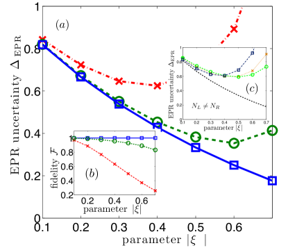
Figure 13: (color online). EPR uncertainty (a) and fidelity $\mathcal{F}$ with the ideal nuclear target state $\left|\xi_{\mathrm{ss}}\right\rangle$ given in Eq.(87) (b) as a function of the squeezing-like parameter $\left|\xi\right|$ for $N_{L}=N_{R}=3$ inhomogeneously coupled nuclei. The blue curve (squares) refers to a symmetric setting where $\vec{a}_{L}=\vec{a}_{R}=\left(1.11,1.67,0.22\right)$, whereas the green (circles) and red (crosses) solutions incorporate asymmetries: $\vec{a}_{L}=\left(1.18,1.61,0.21\right)$, $\vec{a}_{R}=\left(1.11,1.67,0.22\right)$ and $\vec{a}_{L}=\left(1.0,1.5,0.5\right)$, $\vec{a}_{R}=\left(1.24,1.55,0.21\right)$, respectively. (c) Exact results for the asymmetric scenario $N_{L}=2\neq 3=N_{R}$. Here, $\vec{a}_{L}=\left(1.0,1.5\right)$ was held fixed while the green (circles), orange (crosses) and dark blue (squares) curves refer to $\vec{a}_{R}=\left(0.98,1.47,0.05\right)$, $\vec{a}_{R}=\left(0.93,1.39,0.18\right)$ and $\vec{a}_{R}=\left(0.76,1.14,0.60\right)$, respectively; as a benchmark, the black dashed curve refers to the ideal results in the symmetric setting. Due to the absence of degeneracies, the steady state solution $\sigma_{\mathrm{ss}}$ is unique in all cases considered here.

In what follows, we show that our scheme works even in the case of non-uniform coupling, provided that the two dots are sufficiently similar. If the HF coupling constants are completely inhomogeneous, that is $a_{i,j}\neq a_{i,k}$ for all $j\neq k$, but the two dots are identical $\left(a_{1,j}=a_{2,j}\equiv a_{j}\,\forall j=1,2,\dots,N_{L}\equiv N_{R}\equiv N\right)$, such that the nuclear spins can be grouped into pairs according to their HF coupling constants, the two dominant nuclear jump operators $L_{2}$ and $\mathbb{L}_{2}$ simplify to

$$L_{2} = \sum_{j}a_{j}l_{j},\,\,\,\,\,\,\,\,\,\,\mathbb{L}_{2}=\sum_{j}a_{j}\mathbb{l}_{j},$$ (84)

where the nuclear operators $l_{j}=\nu_{2}\sigma_{Lj}^{+}+\mu_{2}\sigma_{Rj}^{+}$ and $\mathbb{l}_{j}=\mu_{2}\sigma_{Lj}^{-}+\nu_{2}\sigma_{Rj}^{-}$ are nonlocal nuclear operators, comprising two nuclear spins that belong to different nuclear ensembles, but have the same HF coupling constant $a_{j}$. For one such pair of nuclear spins, the unique, common nuclear dark state fulfilling

$$l_{j}\left|\xi\right\rangle_{j}=\mathbb{l}_{j}\left|\xi\right\rangle_{j}=0,$$ (85)

is easily verified to be

$$\left|\xi\right\rangle_{j}=\mathcal{N}_{\xi}\left(\left|\downarrow_{j},\uparrow_{j}\right\rangle+\xi\left|\uparrow_{j},\downarrow_{j}\right\rangle\right),$$ (86)

where $\mathcal{N}_{\xi}=1/\sqrt{1+\xi^{2}}$ for normalization. Therefore, in the absence of degeneracies in the HF coupling constants $\left(a_{i,j}\neq a_{i,k}\,\forall j\neq k\right)$, the pure, entangled ideal nuclear dark state fulfilling $L_{2}\left|\xi_{\mathrm{ss}}\right\rangle=\mathbb{L}_{2}\left|\xi_{\mathrm{ss}}\right\rangle=0$ can be constructed as a tensor product of entangled pairs of nuclear spins,

$$\left|\xi_{\mathrm{ss}}\right\rangle=\otimes_{j=1}^{N}\left|\xi\right\rangle_{j}.$$ (87)

Again, the parameter $\xi=-\nu_{2}/\mu_{2}$ fully quantifies polarization and entanglement properties of the nuclear stationary state; compare Eq.(44): First, for small values of the parameter $\left|\xi\right|$ the ideal nuclear dark state $\left|\xi_{\mathrm{ss}}\right\rangle$ features an arbitrarily high polarization gradient

$$\Delta_{I^{z}}=\left\langle I_{R}^{z}\right\rangle_{\mathrm{ss}}-\left\langle I_{L}^{z}\right\rangle_{\mathrm{ss}}=N\frac{1-\xi^{2}}{1+\xi^{2}},$$ (88)

whereas the homogeneous net polarization $P=\left\langle I_{L}^{z}\right\rangle_{\mathrm{ss}}+\left\langle I_{R}^{z}\right\rangle_{\mathrm{ss}}$ vanishes. The stationary solution for the nuclear gradient $\Delta_{I^{z}}$ is bistable as it is positive (negative) for $\left|\xi\right|<1$ $\left(\left|\xi\right|>1\right)$, respectively. Second, the amount of entanglement inherent to the stationary solution $\left|\xi_{\mathrm{ss}}\right\rangle$ can be quantified via the EPR uncertainty ($\Delta_{\mathrm{EPR}}<1$ indicates entanglement) and is given by $\Delta_{\mathrm{EPR}}=\left(1-\left|\xi\right|\right)^{2}/\left|1-\xi^{2}\right|.$

Our analytical findings are verified by exact diagonalization results for small sets of inhomogeneously coupled nuclei. Here, we compute the exact (possibly mixed) solutions $\sigma_{\mathrm{ss}}$ to the dark state equation $\mathcal{D}\left[L_{2}\right]\sigma_{\mathrm{ss}}+\mathcal{D}\left[\mathbb{L}_{2}\right]\sigma_{\mathrm{ss}}=0$; compare Fig. 7 for the special case of uniform HF coupling. As shown in Fig. 13, our numerical evidence indicates that small deviations from the perfect symmetry (that is for $a_{Lj}\approx a_{Rj}$) between the QDs still yield a (mixed) unique entangled steady state close to $\left|\xi_{\mathrm{ss}}\right\rangle$. In the ideal case $a_{Lj}=a_{Rj}$, we recover the pure steady state given in Eq.(87). Moreover, we find that the generation of steady-state entanglement even persists for asymmetric dot sizes, i.e. for $N_{L}\neq N_{R}$. Exact solutions for $N_{L}=2\neq 3=N_{R}$ are displayed in Fig. 13. Here, we still find strong traces of the ideal dark state $\left|\xi_{\mathrm{ss}}\right\rangle$, provided that one can approximately group the nuclear spins into pairs of similar HF coupling strength. The interdot correlations $\left\langle\sigma_{Lj}^{+}\sigma_{Rj}^{-}\right\rangle$ are found to be close to the ideal value of $\xi/\left(1+\xi^{2}\right)$ for nuclear spins with a similar HF constant, but practically zero otherwise. In line with this reasoning, the highest amount of entanglement in Fig. 13 is observed in the case where one of the nuclear spins belonging to the bigger second ensemble is practically uncoupled. Lastly, we note that one can ’continuously’ go from the case of non-degenerate HF coupling constants (the case considered in detail here) to the limit of uniform HF coupling [compare Eq.(44)] by grouping spins with the same HF coupling constants to ’shells’, which form collective nuclear spins. For degenerate couplings, however, there are additional conserved quantities, namely the respective total spin quantum numbers, and therefore multiple stationary states of the above form. As argued in Section III, a mixture of different $J$-subspaces should still be entangled provided that the range of $J$-subspaces involved in this mixture is small compared to the average $J$ value.

Larger nuclear spins.—All natural isotopes of Ga and As carry a nuclear spin $I=3/2$,schliemann03 whereas we have considered $I=1/2$ for the sake of simplicity. For our purposes, however, this effect can easily be incorporated as an individual nuclear spin with $I=3/2$ maps onto 3 homogeneously coupled nuclear spins with individual $I=1/2$ which are already in the fully symmetric Dicke subspace $J=3/2$.

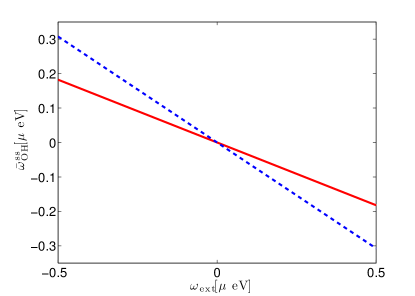
Figure 14: (color online). Buildup of a homogeneous nuclear Overhauser field component $\bar{\omega}_{\mathrm{OH}}^{\mathrm{ss}}$ which partially compensates an applied external magnetic field, shown here for $t=10\mu\mathrm{eV}$ (red solid) and $t=20\mu\mathrm{eV}$ (blue dashed). Other numerical parameters: $\Gamma=25\mu\mathrm{eV}$, $\epsilon=30\mu\mathrm{eV}$, $\Gamma_{\pm}=\Gamma_{\mathrm{deph}}=0.1\mu\mathrm{eV}$.

External magnetic fields.—For simplicity, our previous analysis has focused on a symmetric setting of vanishing external fields, $\Delta_{\mathrm{ext}}=\omega_{\mathrm{ext}}=0$. Non-vanishing external fields, however, may be used as further experimental knobs to tune the desired nuclear steady-state properties: First, as mentioned above, a non-zero external gradient $\Delta_{\mathrm{ext}}$ is beneficial for our proposal as it can provide an efficient way to destabilize the zero-polarization solution $\left(\Delta_{\mathrm{OH}}^{\mathrm{ss}}=0\right)$ by initiating the nuclear self-polarization process. Second, non-vanishing $\omega_{\mathrm{ext}}\neq 0$ gives rise to another electron-nuclear feedback-driven experimental knob for controlling the nuclear stationary state. In the framework of Section IV, for $\omega_{\mathrm{ext}}\neq 0$ the semiclassical dynamical equations can be generalized to

$$\frac{d}{dt}\left\langle I_{L}^{z}\right\rangle_{t} = \alpha_{+}N_{L\downarrow}-\beta_{-}N_{L\uparrow},$$ (89)

$$\frac{d}{dt}\left\langle I_{R}^{z}\right\rangle_{t} = \beta_{+}N_{R\downarrow}-\alpha_{-}N_{R\uparrow},$$ (90)

where we have introduced the number of nuclear spin-up and spin-down spins as $N_{i\uparrow}=N_{i}/2+\left\langle I_{i}^{z}\right\rangle$ and $N_{i\downarrow}=N_{i}/2-\left\langle I_{i}^{z}\right\rangle$, respectively, and the generalized polarization rates

$$\alpha_{\pm} = p\gamma^{\pm}\nu_{2}^{2}+\left(1-2p\right)\gamma^{\mp}\mu_{2}^{2},$$ (91)

$$\beta_{\pm} = p\gamma^{\pm}\mu_{2}^{2}+\left(1-2p\right)\gamma^{\mp}\nu_{2}^{2}.$$ (92)

They depend on the generalized HF-mediated decay rate

$$\gamma^{\pm}=\frac{a_{\mathrm{hf}}^{2}\tilde{\Gamma}}{2\left[\left(\epsilon_{2}\mp\omega_{0}\right)^{2}+\tilde{\Gamma}^{2}\right]},$$ (93)

which accounts for different detunings for $\omega_{0}\neq 0$; compare Eq.(39). As shown in Fig. 14, in the presence of an external magnetic splitting $\omega_{\mathrm{ext}}$, the nuclear spins build up a homogeneous Overhauser field $\bar{\omega}_{\mathrm{OH}}$ in the steady state to partially compensate the external component. The steady state solution then locally fulfills a detailed-balance principle, namely $\alpha_{+}N_{L\downarrow}=\beta_{-}N_{L\uparrow}$ and $\beta_{+}N_{R\downarrow}=\alpha_{-}N_{R\uparrow}$, which is determined by effective nuclear flip rates and the number of spins available for a spin flip. Intuitively, this finding can be understood as follows: For $\omega_{\mathrm{ext}}\neq 0$, the degeneracy between $\left|T_{+}\right\rangle$ and $\left|T_{-}\right\rangle$ is lifted with one of them being less detuned from $\left|\lambda_{2}\right\rangle$ than the other. This favors the build-up of a nuclear net polarization $P$ which, however, counteracts the splitting $\omega_{\mathrm{ext}}$; for $\omega_{\mathrm{ext}}=0$, this mechanism stabilizes $\bar{\omega}_{\mathrm{OH}}=P=0$ in the stationary state. This result has also been confirmed by numerical results presented in Appendix G.

Species inhomogeneity.—Nonzero external magnetic fields, however, induce nuclear Zeeman splittings, with the nuclear magnetic moment being about three orders of magnitude smaller than the Bohr magneton for typical quantum dots.hanson07 ; schliemann03 Most QDs consist of a few (in GaAs three) different species of nuclei with strongly varying $g$ factors. In principle, this species-inhomogeneity can cause dephasing between the nuclear spins. However, for a uniform external magnetic field this dephasing mechanism only applies to nuclei belonging to different species. In a rotating wave approximation, this leads to few mutually decohered subsystems (in GaAs three) each of which being driven towards a two-mode squeezedlike steady state: note that, because of the opposite polarizations in the two dots, the nuclear target state $\left|\xi\right\rangle_{\mathrm{ss}}$ is invariant under the application of a homogeneous magnetic field. This argument, however, does not hold for an inhomogeneous magnetic field which causes dephasing of $\left|\xi\right\rangle_{\mathrm{ss}}$ as the nuclear states $\left|m,-m\right\rangle$ ($m$ is the nuclear spin projection) pick up a phase $\exp\left[2im\Delta_{\mathrm{ext}}^{\mathrm{nuc}}t\right]$, where $\Delta_{\mathrm{ext}}^{\mathrm{nuc}}\approx 10^{-3}\Delta_{\mathrm{ext}}$. If one uses an external magnetic gradient to incite the nuclear self-polarization process, after successful polarization one should therefore switch off the gradientsmall-gradient-entanglement to support the generation of entanglement between the two ensembles.

Weak nuclear interactions.—We have neglected nuclear dipole-dipole interactions among the nuclear spins. The strength of the effective magnetic dipole-dipole interaction between neighboring nuclei in GaAs is about $g_{dd}\sim\left(100\mu\mathrm{s}\right)^{-1}$.hanson07 ; schliemann03 Spin-nonconserving terms and flip-flop terms between different species can be suppressed efficiently by applying an external magnetic field of $B_{\mathrm{ext}}\gtrsim 10\mathrm{mT}$.reilly08 As discussed above, the corresponding (small) electron Zeeman splitting $\omega_{\mathrm{ext}}\approx 0.25\mu\mathrm{eV}$ does not hamper our protocol. Then, it is sufficient to consider so-called homonuclear flip-flop terms between nuclei of the same species only and phase changing $zz$-terms. First, nuclear spin diffusion processes—governing the dynamics of the spatial profile of the nuclear polarization by changing $A_{i}^{z}$—have basically no effect within an (almost) completely symmetric Dicke subspace. With typical timescales of $\gtrsim 10\mathrm{s}$, they are known to be very slow and therefore always negligible on the timescale considered here.reilly08 ; rudner13 ; paget82 Second, the interactions $\propto\sigma_{i}^{z}\sigma_{j}^{z}$ lead to dephasing similar to the nuclear Zeeman terms discussed above: In a mean-field treatment one can estimate the effective Zeeman splitting of a single nuclear spin in the field of its surrounding neighbors to be a few times $g_{dd}$.christ07 This mean field is different only for different species and thus does not cause any homonuclear dephasing. Still, the variance of this effective field may dephase spins of the same species, but for a high nuclear polarization $\text{$\mathrm{p}$}_{\mathrm{nuc}}$ this effect is further suppressed by a factor $\sim\left(1-\mathrm{p}_{\mathrm{nuc}}^{2}\right)$ as the nuclei experience a sharp field for a sufficiently high nuclear polarization $\text{$\mathrm{p}$}_{\mathrm{nuc}}$. Lastly, we refer to recently measured nuclear decoherence times of $\sim 1\mathrm{ms}$ in vertical double quantum dots.takahashi11 Since this is slow compared to the dissipative gap of the nuclear dynamics $\tau_{\mathrm{gap}}\approx\left(3-30\right)\mu\mathrm{s}$ for $N\approx 10^{5}-10^{6}$, we conclude that it should be possible to create entanglement between the two nuclear spin ensembles faster than it gets disrupted due to dipole-dipole interactions among the nuclear spins or other competing mechanisms.rudner11a Moreover, since strain is largely absent in electrically defined QDs,chekhovich13 nuclear quadrupolar interactions have been neglected as well. For a detailed analysis of the internal nuclear dynamics within a HP treatment, we refer to Ref.schwager10 .

Charge noise.—Nearly all solid-state qubits suffer from some kind of charge noise.dial13 In a DQD device background charge fluctuations and noise in the gate voltages may cause undesired dephasing processes. In a recent experimental study,dial13 voltage fluctuations in $\epsilon$ have been identified as the source of the observed dephasing in a singlet-triplet qubit. In our setting, however, the electronic subsystem quickly settles into the quasisteady state $\rho_{\mathrm{ss}}^{\mathrm{el}}$ which lives solely in the $\left(1,1\right)$ triplet subspace spanned by $\left\{\left|T_{\pm}\right\rangle\right\}$ and is thus relatively robust against charge noise. Still, voltage fluctuations in $\epsilon$ lead to fluctuations in the parameter $\xi$ characterizing the nuclear two-mode target state given in Eq.(44). For typical parameters $\left(t=20\mu\mathrm{eV},\,\epsilon=30\mu\mathrm{eV},\,\Delta=40\mu\mathrm{eV}\right)$, however, $\xi$ turns out to be rather insensitive to fluctuations in $\epsilon$, that is $\left|d\xi/d\epsilon\right|\approx 10^{-2}/\mu\mathrm{eV}$. Note that the system can be made even more robust (while keeping $\xi$ constant) by increasing both $\epsilon$ and $t$: For $t=50\mu\mathrm{eV}$, $\epsilon=90\mu\mathrm{eV}$, the charge noise sensitivity is further reduced to $\left|d\xi/d\epsilon\right|\approx 3\times 10^{-3}/\mu\mathrm{eV}$. We can then estimate the sensitivity of the generated steady-state entanglement via $\left|d\Delta_{\mathrm{EPR}}/d\epsilon\right|=\left|(d\xi/d\epsilon)(d\Delta_{\mathrm{EPR}}/d\xi)\right|\lesssim 2\times 10^{-2}/\mu\mathrm{eV}$, where we have used $\left|d\Delta_{\mathrm{EPR}}/d\xi\right|=2/\left(1+\xi\right)^{2}<2$. Typical fluctuations in $\epsilon$ of the order of $\sim\left(1-3\right)\mu\mathrm{eV}$ as reported in Ref.hayashi03 may then cause a reduction of entanglement in the nuclear steady state of approximately $\sim 5\%$ as compared to the optimal value of $\epsilon$. If the typical timescale associated with charge noise $\tau_{\mathrm{noise}}$ is fast compared to the dissipative gap of the nuclear dynamics, i.e., $\tau_{\mathrm{noise}}\ll\tau_{\mathrm{gap}}$, the nuclear spins effectively only experience the averaged value of $\xi$, coarse-grained over its fast fluctuations.

VIII Conclusion and Outlook

In summary, we have developed a theoretical master-equation-based framework for a DQD in the Pauli-blockade regime which features coupled dynamics of electron and nuclear spins as a result of the hyperfine interaction. Our analysis is based on the typical separation of timescales between (fast) electron spin evolution and (slow) nuclear spin dynamics, yielding a coarse-grained quantum master equation for the nuclear spins. This reverses the standard perspective in which the nuclei are considered as an environment for the electronic spins, but rather views the nuclear spins as the quantum system coupled to an electronic environment with an exceptional degree of tunability. Here, we have focused on a regime favorable for the generation of entanglement in the nuclear steady state, whereas the electrons are driven to an unpolarized, classically correlated separable state. Therefore, in this setting, electron dephasing turns out to be an asset rather than a liability. Our central master equation directly incorporates nonlinear feedback mechanisms resulting from the back-action of the Overhauser field on the electron energy levels and thus explains the nuclear multi-stability in a very transparent way. The associated instability of the nuclei towards self-polarization can be used as a means for controlling the nuclear spin distribution.rudner07 For example, as a prominent application, we predict the deterministic generation of entanglement between two (spatially separated) mesoscopic spin ensembles, induced by electron transport and the common, collective coupling of the nuclei to the electronic degrees of freedom of the DQD. The nuclear entangled state is of EPR type, which is known to play a key role in continuous variable quantum information processinghammerer10 ; furusawa07 , quantum sensingwasilewski10 and metrologyappel09 ; schleier-smith10 ; gross10 . Since the entanglement generation does not rely on coherent evolution, but is rather stabilized by the dissipative dynamics, the proposed scheme is inherently robust against weak random perturbations. Moreover, as two large spin ensembles with $N\sim 10^{6}$ get entangled, the nuclear system has the potential to generate large amounts of entanglement, i.e., many ebits. Lastly, the apparent relatively large robustness of the nuclear steady state against charge noise shows that, when viewed as (for example) a platform for spin-based quantum memories, nuclear spin ensembles have certain, intrinsic advantages with respect to their electronic cousins.

Our results provide a clear picture of the feedback-driven polarization dynamics in a generic electron transport setting and, therefore, should serve as a useful guideline for future experiments aiming at an enhanced, dynamical control of the nuclear spins: While DNP experiments in double quantum dots, for example, have revealed an instability towards large Overhauser gradients, consistent with our results, the question of whether or not this instability results from dot asymmetry or some other mechanism is still unsettled.foletti09 ; petta08 ; barthel12 Here, we study a generic DC setting, where the buildup of a large OH gradient straightforwardly emerges even in the presence of a completely symmetric coherent hyperfine interaction. From a more fundamental, conceptual point of view, our theory gives valuable insights into the complex, non-equilibrium many-body dynamics of localized electronic spins interacting with a mesoscopic number of nuclear spins. Understanding the quantum dynamics of this central spin model marks an important goal in the field of mesoscopic physics, as a notable number of unexpected and intriguing phenomena such as multi-stability, switching, hysteresis and long timescale oscillations have been observed in this system.ono04 ; koppens05 ; danon09b ; rudner13

On the one hand, reversing again our approach, our scheme may lead to a better quantum control over the nuclear spin bath and therefore improved schemes to coherently control electron spin qubits, by reducing the Overhauser field fluctuations and/or exploiting the gradient for electron spin manipulation (as demonstrated experimentally already for example in Ref.foletti09 ). On the other hand, with nuclear spin coherence times ranging from hundreds of microseconds to a millisecond,takahashi11 ; chekhovich13 our work could be extended towards nuclear spin-based information storage and manipulation protocols. The nuclear spin ensembles could serve as a long-lived entanglement resource providing the basic building block for an on-chip (solid-state) quantum network. The nodes of this quantum network could be interconnected with electrons playing the role of photons in more conventional atomic, molecular, and optical (AMO) based approaches.kimble08 To wire up the system, coherent transport of electron spins over long distances (potentially tens of microns in state-of-the-art experimental setups) could be realized via QD arrays busl13 ; braakman13 , quantum Hall edge channelsfletcher13 ; feve07 ; bocquillon13 ; roulleau08 ; mahe10 or surface acoustic waveshermelin11 ; mcneil11 ; sanada13 ; yamamoto12 . Building upon this analogy to quantum optics, the localized nuclei might also be used as a source to generate a current of many entangled electrons.christ08 Using the aforementioned tunability of the electronic degrees of freedom, one could also engineer different electronic quasisteady states, possibly resulting in nuclear stationary states with on-demand properties. On a more fundamental level, our work could also be extended towards deeper studies of dissipative phase transitions in this rather generic transport setting. When combined with driving—realized via, for example, a magnetic field $B_{x}$ perpendicular to the polarization direction—a variety of strong-correlation effects, nonequilibrium, and dissipative phase transitions can be expectedkessler12 ; carmichael80 ; morrison08 and could now be studied in a mesoscopic solid-state system, complementing other approaches to dissipative phase transitions in quantum dotsrudner10 ; chung09 ; borda06 ; leggett87 .

Appendix A Spin-Blockade Regime

In this appendix, for completeness we explicitly derive inequalities involving the chemical potentials $\mu_{L\left(R\right)}$ of the left and right lead, respectively, as well as the Coulomb energies introduced in Eq.(7) that need to be satisfied in order to tune the DQD into the desired Pauli-blockade regime in which at maximum two electrons reside on the DQD. For simplicity, Zeeman splittings are neglected for the moment as they typically constitute a much smaller energy scale compared to the Coulomb energies. Still, an extension to include them is straight-forward. Then, the bare energies $E_{\left(m,n\right)}$ for a state with $\left(m,n\right)$ charge configuration can easily be read off from the Anderson Hamiltonian $H_{S}$. In particular, we obtain

$$E_{\left(1,1\right)} = \epsilon_{L}+\epsilon_{R}+U_{LR},$$ (94)

$$E_{\left(2,1\right)} = 2\epsilon_{L}+\epsilon_{R}+U_{L}+2U_{LR},$$ (95)

$$E_{\left(1,2\right)} = \epsilon_{L}+2\epsilon_{R}+U_{R}+2U_{LR},$$ (96)

$$E_{\left(0,2\right)} = 2\epsilon_{R}+U_{R},$$ (97)

$$E_{\left(2,0\right)} = 2\epsilon_{L}+U_{L}.$$ (98)

In order to exclude the occupation of $\left(2,1\right)$ and $\left(1,2\right)$ states if the DQD is in a $\left(1,1\right)$ charge configuration the left chemical potential must fulfill the inequality $\mu_{L}<E_{\left(2,1\right)}-E_{\left(1,1\right)}=\epsilon_{L}+U_{L}+U_{LR}$. An analog condition needs to be satisfied for the right chemical potential $\mu_{R}$ so that we can write in total

$$\mu_{i}<\epsilon_{i}+U_{i}+U_{LR}.$$ (99)

The same requirement should hold if the DQD is in a $\left(0,2\right)$ or $\left(2,0\right)$ charge configuration which leads to

$$\mu_{i}<\epsilon_{i}+2U_{LR}.$$ (100)

At the same time, the chemical potentials $\mu_{i}$ are tuned sufficiently high so that an electron is added to the DQD from the leads whenever only a single electron resides in the DQD. For example, this results in $\mu_{L}>E_{\left(1,1\right)}-\epsilon_{R}=\epsilon_{L}+U_{LR}$. An analog condition needs to hold for the right lead which gives

$$\mu_{i}>\epsilon_{i}+U_{LR}.$$ (101)

In particular this inequality guarantees that the right dot is always occupied, since $\mu_{R}>\epsilon_{R}$. Moreover, localized singlet states cannot populated directly if $\mu_{i}<\epsilon_{i}+U_{i}$ holds. Since $U_{LR}<U_{i}$, the conditions to realize the desired two-electron regime can be summarized as

$$\epsilon_{i}+U_{LR}<\mu_{i}<\epsilon_{i}+2U_{LR}.$$ (102)

By applying a large bias that approximately compensates the charging energy of the two electrons residing on the right dot, that is $\epsilon_{L}\approx\epsilon_{R}+U_{R}-U_{LR}$, the occupation of a localized singlet with charge configuration $\left(2,0\right)$ can typically be neglected.stepaneko12 ; rudner10 In this regime, only states with the charge configurations $\left(0,1\right)$, $\left(1,0\right)$, $\left(1,1\right)$ and $\left(0,2\right)$ are relevant. Also, due to the large bias, admixing within the one-electron manifold is strongly suppressed—for typical parameters we estimate $t/\left(\epsilon_{L}-\epsilon_{R}\right)\approx 10^{-2}$—such that the relevant single electron states that participate in the transport cycle in the spin-blockade regime are the two lowest ones $\left|0,\sigma\right\rangle=d_{R\sigma}^{\dagger}\left|0\right\rangle$ with $\left(0,1\right)$ charge configuration.giavaras13

Appendix B Quantum Master Equation in Spin-Blockade Regime

Following the essential steps presented in Ref.schuetz12 , we now derive an effective master equation for the DQD system which experiences irreversible dynamics via the electron’s coupling to the reservoirs in the leads. We start out from the von Neumann equation for the global density matrix given in Eq.(18). It turns out to be convenient to decompose $\mathcal{H}$ as

$$\mathcal{H}=H_{0}+H_{1}+H_{T},$$ (103)

with $H_{0}=H_{S}+H_{B}$ and $H_{1}=V_{\mathrm{HF}}+H_{t}$. We define the superoperator $P$ as

$$P\varrho=\mathsf{Tr}_{\mathsf{B}}\left[\varrho\right]\otimes\rho_{B}^{0}.$$ (104)

It acts on the total system’s density matrix $\varrho$ and projects the environment onto their respective thermal equilibrium states, labeled as $\rho_{B}^{0}$. The map $P$ satisfies $P^{2}=P$ and is therefore called a projector. By deriving a closed equation for the projection $P\varrho$ and tracing out the unobserved reservoir degrees of freedom, we arrive at the Nakajima-Zwanzig master equation for the system’s density matrix

$$\dot{\rho} = \left[\mathcal{L}_{S}+\mathcal{L}_{1}\right]\rho$$

$$+\int_{0}^{t}d\tau\mathsf{Tr}_{\mathsf{B}}\left[\mathcal{L}_{T}e^{\left(\text{$\mathcal{L}$}_{0}+\mathcal{L}_{T}+\mathcal{L}_{1}\right)\tau}\mathcal{L}_{T}\rho\left(t-\tau\right)\otimes\rho_{B}^{0}\right].$$

where the Liouville superoperators are defined as usual via $\mathcal{L}_{\alpha}\cdot=-i\left[H_{\alpha},\cdot\right]$. Next, we introduce two approximations: First, in the weak coupling limit, we neglect all orders higher than two in $\mathcal{L}_{T}$. This is well known as the Born approximation. Accordingly, we neglect $\mathcal{L}_{T}$ in the exponential of the integrand. Second, we apply the approximation of independent rates of variations cohen-tannoudji92 which can be justified self-consistently, if the bath correlation time $\tau_{c}$ is short compared to the typical timescales associated with the system’s internal interactions, that is $g_{\mathrm{hf}}\tau_{c}\ll 1$ and $t\tau_{c}\ll 1$, and if $H_{1}$ can be treated as a perturbation with respect to $H_{0}$. In our system, the latter is justified as $H_{0}$ incorporates the large Coulomb energy scales which energetically separate the manifold with two electrons on the DQD from the lower manifold with only one electron residing in the DQD, whereas $H_{1}$ induces couplings within these manifolds only. In this limit, the master equation then reduces to

$$\dot{\rho} = \left[\mathcal{L}_{S}+\mathcal{L}_{1}\right]\rho$$

$$+\int_{0}^{t}d\tau\mathsf{Tr}_{\mathsf{B}}\left[\mathcal{L}_{T}e^{\text{$\mathcal{L}$}_{0}\tau}\mathcal{L}_{T}\rho\left(t-\tau\right)\otimes\rho_{B}^{0}\right].$$

In the next step, we write out the tunnel Hamiltonian $H_{T}$ in terms of the relevant spin-eigenstates. Here, we single out one term explicitly, but all others follow along the lines. We get

$$\dot{\rho} = \dots+\sum_{\sigma}\int_{0}^{t}d\tau\mathcal{C}\left(\tau\right)\left|0,\sigma\right\rangle\left\langle S_{02}\right|$$

$$\left[e^{-iH_{0}\tau}\rho\left(t-\tau\right)e^{iH_{0}\tau}\right]\left|S_{02}\right\rangle\left\langle 0,\sigma\right|,$$

where

$$\mathcal{C}\left(\tau\right)=\int_{0}^{\infty}d\epsilon J\left(\epsilon\right)e^{i\left(\Delta E-\epsilon\right)\tau},$$ (108)

and $J\left(\epsilon\right)=\left|T_{R}\right|^{2}n_{R}\left(\epsilon\right)\left[1-f_{R}\left(\epsilon\right)\right]$ is the spectral density of the right lead, with $n_{R}\left(\epsilon\right)$ being the density of states per spin of the right lead; $f_{\alpha}\left(\epsilon\right)$ denotes the Fermi function of lead $\alpha=L,R$ and $\Delta E$ is the energy splitting between the two levels involved, i.e., for the term explicitly shown above $\Delta E=\epsilon_{R}+U_{R}$. The correlation time of the bath $\tau_{c}$ is determined by the decay of the memory-kernel $\mathcal{C}\left(\tau\right)$. The Markov approximation is valid if the spectral density $J\left(\epsilon\right)$ is flat on the scale of all the effects that we have neglected in the previous steps. Typically, the effective density of states $D\left(\epsilon\right)=\left|T_{R}\right|^{2}n_{R}\left(\epsilon\right)$ is weakly energy dependent so that this argument is mainly concerned with the Fermi functions of the left (right) lead $f_{L\left(R\right)}\left(\epsilon\right)$, respectively. Therefore, if $f_{i}\left(\epsilon\right)$ is flat on the scale of $\sim t$, $\sim g_{\mathrm{hf}}$ and the dissipative decay rates $\sim\Gamma$, it can be evaluated at $\Delta E$ and a Markovian treatment is valid.schuetz12 In summary, this results in

$$\dot{\rho}=\dots+\Gamma_{R}\sum_{\sigma}\mathcal{D}\left[\left|0,\sigma\right\rangle\left\langle S_{02}\right|\right]\rho,$$ (109)

where $\Gamma_{R}$ is the typical sequential tunneling rate $\Gamma_{R}=2\pi\left|T_{R}\right|^{2}n_{R}\left(\Delta E\right)\left[1-f_{R}\left(\Delta E\right)\right]$ describing direct hopping at leading order in the dot-lead coupling.qassemi09 ; schuetz12

Pauli blockade.—The derivation above allows for a clear understanding of the Pauli-spin blockade in which only the level $\left|S_{02}\right\rangle$ can decay into the right lead whereas all two electron states with $\left(1,1\right)$ charge configuration are stable. If the $\left|S_{02}\right\rangle$ level decays, an energy of $\Delta E_{2}=E_{\left(0,2\right)}-\epsilon_{R}=\epsilon_{R}+U_{R}$ is released on the DQD which has to be absorbed by the right reservoir due to energy conservation arguments. On the contrary, if one of the $\left(1,1\right)$ levels were to decay to the right lead, an energy of $\Delta E_{1}=E_{\left(1,1\right)}-\epsilon_{L}=\epsilon_{R}+U_{LR}$ would dissipate into the continuum. Therefore, the DQD is operated in the Pauli blockade regime if $f_{R}\left(\Delta E_{2}\right)=0$ and $f_{R}\left(\Delta E_{1}\right)=1$ is satisfied. Experimentally, this can be realized easily as $\Delta E_{2}$ scales with the on-site Coulomb energy $\Delta E_{2}\sim U_{R}$, whereas $\Delta E_{1}$ scales only with the interdot Coulomb energy $\Delta E_{1}\sim U_{LR}$.

Taking into account all relevant dissipative processes within the Pauli-blockade regime and assuming the Fermi function of the left lead $f_{L}\left(\epsilon\right)$ to be sufficiently flat, the full quantum master equation for the DQD reads

$$\dot{\rho} = -i\left[H_{S}+H_{1},\rho\right]+\Gamma_{R}\sum_{\sigma}\mathcal{D}\left[\left|0,\sigma\right\rangle\left\langle S_{02}\right|\right]\rho$$ (110)

$$+\Gamma_{L}\left\{\mathcal{D}\left[\left|T_{+}\right\rangle\left\langle 0,\Uparrow\right|\right]\rho+\mathcal{D}\left[\left|\Downarrow\Uparrow\right\rangle\left\langle 0,\Uparrow\right|\right]\rho\right\}$$

$$+\Gamma_{L}\left\{\mathcal{D}\left[\left|T_{-}\right\rangle\left\langle 0,\Downarrow\right|\right]\rho+\mathcal{D}\left[\left|\Uparrow\Downarrow\right\rangle\left\langle 0,\Downarrow\right|\right]\rho\right\},$$

where the rate $\Gamma_{R}\sim\left[1-f_{R}\left(\Delta E_{2}\right)\right]$ describes the decay of the localized singlet $\left|S_{02}\right\rangle$ into the right lead, while the second and third line represent subsequent recharging of the DQD with the corresponding rate $\Gamma_{L}\propto\left|T_{L}\right|^{2}$.secular-approximation

We can obtain a simplified description for the regime in which on relevant timescales the DQD is always populated by two electrons. This holds for sufficiently strong recharging of the DQD which can be implemented experimentally by making the left tunnel barrier $T_{L}$ more transparent than the right one $T_{R}$.schuetz12 ; petersen13 ; giavaras13 In this limit, we can eliminate the intermediate stage in the sequential tunneling process $\left(0,2\right)\rightarrow\left(0,1\right)\rightarrow\left(1,1\right)$ and parametrize $H_{S}+H_{1}$ in the two-electron regime as $H_{\mathrm{el}}+H_{\mathrm{ff}}+H_{\mathrm{zz}}$. Then, we arrive at the effective master equation

$$\dot{\rho}=-i\left[H_{\mathrm{el}},\rho\right]+\mathcal{K}_{\Gamma}\rho+\mathcal{V}\rho,$$ (111)

where the dissipator

$$\mathcal{K}_{\Gamma}\rho=\Gamma\sum_{x\in\left(1,1\right)}\mathcal{D}\left[\left|x\right\rangle\left\langle S_{02}\right|\right]\rho$$ (112)

models electron transport through the DQD; the sum runs over all four electronic bare levels with $\left(1,1\right)$ charge configuration, i.e., $\left|\sigma,\sigma^{\prime}\right\rangle$ for $\sigma,\sigma^{\prime}=\Uparrow,\Downarrow$: Thus, in the limit of interest, the $\left(1,1\right)$ charge states are reloaded with an effective rate $\Gamma=\Gamma_{R}/2$ via the decay of the localized singlet $\left|S_{02}\right\rangle$.petersen13 ; giavaras13

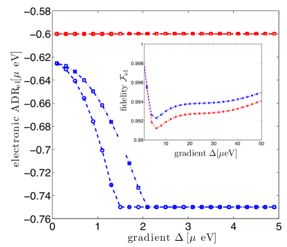
Figure 15: (color online). Electronic asymptotic decay rate $\mathrm{ADR}_{\mathrm{el}}$ and fidelity $\mathcal{F}_{\mathrm{el}}$ for the purely electronic Lindblad dynamics: The results obtained for the full dissipator given in Eq.(B) (circles) are in good agreement with the results we get for the simplified description as stated in Eq.(116) (squares). The blue and red curves correspond to $\Gamma=25\mu\mathrm{eV}$, $\Gamma_{\pm}=0.25\mu\mathrm{eV}$, $\Gamma_{\mathrm{deph}}=0.5\mu\mathrm{eV}$ and $\Gamma=25\mu\mathrm{eV}$, $\Gamma_{\pm}=0.3\mu\mathrm{eV}$, $\Gamma_{\mathrm{deph}}=0$, respectively. Inset: The fidelity $\mathcal{F}_{\mathrm{el}}$ as a figure of merit for the similarity between the quasi-steady-state solutions $\rho_{\mathrm{ss}}^{\mathrm{el}}$ and $\tilde{\rho}_{\mathrm{ss}}^{\mathrm{el}}$, respectively. Other numerical parameters are: $t=20\mu\mathrm{eV}$, $\epsilon=30\mu\mathrm{eV}$ and $\omega_{0}=0$.

Transport dissipator in eigenbasis of $H_{\mathrm{el}}$.—The electronic transport dissipator $\mathcal{K}_{\Gamma}$ as stated in Eq.(112) describes electron transport in the bare basis of the two-orbital Anderson Hamiltonian which does not correspond to the eigenbasis of $H_{\mathrm{el}}$ due to the presence of the interdot tunnel coupling $H_{t}$; in deriving Eq.(112) admixing due to $H_{t}$ has been neglected based on the approximation of independent rates of variation.cohen-tannoudji92 It is valid if $t\tau_{c}\ll 1$ where $\tau_{c}\approx 10^{-15}\text{$\mathrm{s}$}$ specifies the bath correlation time.schuetz12 Performing a basis transformation $\tilde{\rho}=V^{\dagger}\rho V$ which diagonalizes the electronic Hamiltonian $\tilde{H}_{\mathrm{el}}=V^{\dagger}H_{\mathrm{el}}V=\mathrm{diag}\left(\omega_{0},-\omega_{0},\epsilon_{1},\epsilon_{2},\epsilon_{3}\right)$ and neglecting terms rotating at a frequency of $\epsilon_{l}-\epsilon_{k}$ for $k\neq l$, the electronic transport dissipator takes on the formtilde

$$\mathcal{K}_{\Gamma}\tilde{\rho} = \sum_{k,\nu=\pm}\Gamma_{k}\mathcal{D}\left[\left|T_{\nu}\right\rangle\left\langle\lambda_{k}\right|\right]\tilde{\rho}$$

$$+\sum_{k,j}\Gamma_{k\rightarrow j}\mathcal{D}\left[\left|\lambda_{j}\right\rangle\left\langle\lambda_{k}\right|\right]\tilde{\rho},$$

where $\Gamma_{k}=\kappa_{k}^{2}\Gamma$ and $\Gamma_{k\rightarrow j}=\Gamma_{k}[1-\left|\kappa_{j}\right|^{2}]$. Since only $\left(1,1\right)$ states can be refilled, the rate at which the level $\left|\lambda_{j}\right\rangle$ is populated is proportional to $\sim[1-\left|\kappa_{j}\right|^{2}]$; compare Ref.petersen13 . While the first line in Eq.(B) models the decay from the dressed energy eigenstates $\left|\lambda_{k}\right\rangle$ back to the Pauli-blocked triplet subspace $\left|T_{\nu}\right\rangle\left(\text{$\nu$=$\pm$}\right)$ with an effective rate according to their overlap with the localized singlet, the second line refers to decay and dephasing processes acting entirely within the ’fast’ subspace spanned by $\left\{\left|\lambda_{k}\right\rangle\right\}$. Intuitively, they should not affect the nuclear dynamics that take place on a much longer timescale. This intuitive picture is corroborated by exact diagonalization results: Leaving the HF interaction $\mathcal{V}$ aside for the moment, we compare the dynamics $\dot{\rho}=\mathcal{K}_{0}\rho$ generated by the full electronic Liouvillian

$$\mathcal{K}_{0}\rho = -i\left[H_{\mathrm{el}},\rho\right]+\mathcal{K}_{\Gamma}\rho$$

$$+\mathcal{K}_{\text{$\pm$}}\rho+\mathcal{L}_{\mathrm{deph}}\rho,$$

$$\mathcal{K}_{\text{$\pm$}}\rho = \Gamma_{\pm}\sum_{\nu=\pm}\mathcal{D}\left[\left|T_{\bar{\nu}}\right\rangle\left\langle T_{\nu}\right|\right]\rho$$

$$+\Gamma_{\pm}\sum_{\nu=\pm}\left[\mathcal{D}\left[\left|T_{\nu}\right\rangle\left\langle T_{0}\right|\right]\rho+\mathcal{D}\left[\left|T_{0}\right\rangle\left\langle T_{\nu}\right|\right]\rho\right]$$

formulated in terms of the five undressed, bare levels $\left\{\left|\sigma,\sigma^{\prime}\right\rangle,\left|S_{02}\right\rangle\right\}$ to the following Liouvillian

$$\mathcal{L}_{0}\tilde{\rho} = -i\left[\tilde{H}_{\mathrm{el}},\tilde{\rho}\right]+\mathcal{L}_{\Gamma}\tilde{\rho}$$ (116)

$$+\mathcal{L}_{\pm}\tilde{\rho}+\mathcal{L}_{\mathrm{deph}}\tilde{\rho},$$

which is based on the simplified form as stated in Eq.(B).cotunneling-dressed-vs-bare Here, we have also disregarded all dissipative processes acting entirely within the fast subspace, that is all terms of the form $\mathcal{D}\left[\left|\lambda_{j}\right\rangle\left\langle\lambda_{k}\right|\right]$; see the second line in Eq.(B). First, as shown in Fig. 15, we have checked numerically that both $\mathcal{K}_{0}$ and $\mathcal{L}_{0}$ feature very similar electronic quasisteady states, fulfilling $\mathcal{K}_{0}\left[\rho_{\mathrm{ss}}^{\mathrm{el}}\right]=0$ and $\mathcal{L}_{0}\left[\tilde{\rho}_{\mathrm{ss}}^{\mathrm{el}}\right]=0$, respectively, with a Uhlmann fidelityuhlmann76 $\mathcal{F}_{\mathrm{el}}\left(\rho_{\mathrm{ss}}^{\mathrm{el}},\tilde{\rho}_{\mathrm{ss}}^{\mathrm{el}}\right)=\left\|\sqrt{\rho_{\mathrm{ss}}^{\mathrm{el}}}\sqrt{\tilde{\rho}_{\mathrm{ss}}^{\mathrm{el}}}\right\|_{\mathrm{tr}}$ exceeding $99\%$; here, $\left\|\cdot\right\|_{\mathrm{tr}}$ is the trace norm, the sum of the singular values. Second, we examine the electronic asymptotic decay rate $\mathrm{ADR}_{\mathrm{el}}$, corresponding to the eigenvalue with the largest real part different from zero, which quantifies the typical timescale on which the electronic subsystem reaches its quasi-steady state.kessler12 In other words, the $\mathrm{ADR}_{\mathrm{el}}$ gives the spectral gap of the electronic Liouvillian $\mathcal{K}_{0}\left(\mathcal{L}_{0}\right)$ setting the inverse relaxation time towards the steady state and therefore characterizes the long-time behaviour of the electronic system. The two models produce very similar results: Depending on the particular choice of parameters, the electronic $\mathrm{ADR}_{\mathrm{el}}$ is set either by the eigenvectors $\left|\lambda_{2}\right\rangle\left\langle T_{\pm}\right|$, $\left|T_{+}\right\rangle\left\langle T_{-}\right|$ and $\left|T_{+}\right\rangle\left\langle T_{+}\right|-\left|T_{-}\right\rangle\left\langle T_{-}\right|$ which explains the kinks observed in Fig. 15 as changes of the eigenvectors determining the $\mathrm{ADR}_{\mathrm{el}}$. In summary, both the electronic quasisteady state $\left(\rho_{\mathrm{ss}}^{\mathrm{el}}\approx\tilde{\rho}_{\mathrm{ss}}^{\mathrm{el}}\right)$ and the electronic asymptotic decay rate $\mathrm{ADR}_{\mathrm{el}}$ are well captured by the approximative Liouvillian given in Eq.(116). Further arguments justifying this approximation are provided in Appendix C.

Appendix C Transport-Mediated Transitions In Fast Electronic Subspace

In this appendix, we provide analytical arguments why one can drop the second line in Eq.(B) and keep only the first one to account for a description of electron transport in the eigenbasis of $H_{\mathrm{el}}$. The second line, given by

$$\mathcal{L}_{\mathrm{fast}}\rho=\sum_{k,j}\Gamma_{k\rightarrow j}\mathcal{D}\left[\left|\lambda_{j}\right\rangle\left\langle\lambda_{k}\right|\right]\rho,$$ (117)

describes transport-mediated transitions in the fast subspace $\left\{\left|\lambda_{k}\right\rangle\right\}$. The transition rate $\Gamma_{k\rightarrow j}=\kappa_{k}^{2}\left[1-\kappa_{j}^{2}\right]\Gamma$ refers to a transport-mediated decay process from $\left|\lambda_{k}\right\rangle$ to $\left|\lambda_{j}\right\rangle$. Here, we show that $\mathcal{L}_{\mathrm{fast}}$ simply amounts to an effective dephasing mechanism which can be absorbed into a redefinition of the effective transport rate $\Gamma$.

The only way our model is affected by $\mathcal{L}_{\mathrm{fast}}$ is that it adds another dephasing channel for the coherences $\left|\lambda_{k}\right\rangle\left\langle T_{\pm}\right|$ which are created by the hyperfine flip-flop dynamics; see Appendix H. In fact, we have

$$\mathcal{L}_{\mathrm{fast}}\left[\left|\lambda_{k}\right\rangle\left\langle T_{\pm}\right|\right] = -\Gamma_{\mathrm{fast},k}\left|\lambda_{k}\right\rangle\left\langle T_{\pm}\right|,$$ (118)

$$\Gamma_{\mathrm{fast},k} = \frac{1}{2}\sum_{j}\Gamma_{k\rightarrow j}.$$ (119)

Due to the normalization condition $\sum_{j}\kappa_{j}^{2}=1$, the new effective dephasing rate $\Gamma_{\mathrm{fast},k}$ is readily found to coincide with the effective transport rate $\Gamma_{k}$, that is $\Gamma_{\mathrm{fast},k}=\Gamma_{k}=\kappa_{k}^{2}\Gamma$. This equality is readily understood since all four $\left(1,1\right)$ levels are populated equally. While $\Gamma_{k}$ describes the decay to the two Pauli-blocked triplet levels, $\Gamma_{\mathrm{fast},k}$ accounts for the remaining transitions within the $\left(1,1\right)$ sector. Therefore, when accounting for $\mathcal{L}_{\mathrm{fast}}$, the total effective dephasing rates $\tilde{\Gamma}_{k}$ needs to be modified as $\tilde{\Gamma}_{k}\rightarrow\tilde{\Gamma}_{k}+\Gamma_{k}=2\Gamma_{k}+3\Gamma_{\pm}+\Gamma_{\mathrm{deph}}/4$. The factor of $2$ is readily absorbed into our model by a simple redefinition of the overall transport rate $\Gamma\rightarrow 2\Gamma$.

Appendix D Electronic Lifting of Pauli-Blockade

This appendix provides a detailed analysis of purely electronic mechanisms which can lift the Pauli-blockade without affecting directly the nuclear spins. Apart from cotunneling processes discussed in the main text, here we analyze virtual spin exchange processes and spin-orbital effects.rudner07 ; rudner11b It is shown, that these mechanisms, though microscopically distinct, phenomenologically amount to effective incoherent mixing and pure dephasing processes within the $(1,1)$ subspace which, for the sake of theoretical generality, are subsumed under the term in Eq.(1).

Let us also note that electron spin resonance (ESR) techniques in combination with dephasing could be treated on a similar footing. As recently shown in Ref.sanchez13 , in the presence of a gradient $\Delta$, ESR techniques can be used to drive the electronic system into the entangled steady state $\left|-\right\rangle=\left(\left|T_{+}\right\rangle-\left|T_{-}\right\rangle\right)/\sqrt{2}$. Magnetic noise may then be employed to engineer the desired electronic quasisteady state.

D.1 Spin Exchange with the Leads

In the Pauli-blockade regime the $\left(1,1\right)$ triplet states $\left|T_{\pm}\right\rangle$ do not decay directly, but—apart from the cotunneling processes described in the main text—they may exchange electrons with the reservoirs in the leads via higher-order virtual processes.rudner07 ; rudner11b We now turn to these virtual, spin-exchange processes which can be analyzed along the lines of the interdot cotunneling effects. Again, for concreteness we fix the initial state of the DQD to be $\left|T_{+}\right\rangle$ and, based on the approximation of independent rates of variationcohen-tannoudji92 , explain the physics in terms of the electronic bare states. The spin-blocked level $\left|T_{+}\right\rangle$ can virtually exchange an electron spin with the left lead yielding an incoherent coupling with the state $\left|\Downarrow\Uparrow\right\rangle$; this process is mediated by the intermediate singly occupied DQD level $\left|0,\Uparrow\right\rangle$ where no electron resides on the left dot. Then, from $\left|\Downarrow\Uparrow\right\rangle$ the system may decay back to the $\left(1,1\right)$ subspace via the localized singlet $\left|S_{02}\right\rangle$. Therefore, for this analysis, in Fig. 3 we simply have to replace $\left|T_{+}(0,2)\right\rangle$ and $\Gamma_{\mathrm{ct}}$ by $\left|0,\Uparrow\right\rangle$ and $\Gamma_{\mathrm{se}}$, respectively. Along the lines of our previous analysis of cotunneling within the DQD, the bottleneck of the overall process is set by the first step, labeled as $\Gamma_{\mathrm{se}}$. The main purpose of this Appendix is an estimate for the rate $\Gamma_{\mathrm{se}}$.

The effective spin-exchange rate can be calculated in a “golden rule” approach in which transitions for different initial and final reservoir states are weighted according to the respective Fermi distribution functions and added incoherently;kouwenhoven97 for more details, see Refs.engel02 ; recher00 . Up to second order in $H_{T}$, the cotunneling rate $\Gamma_{\mathrm{se}}$ for the process $\left|T_{+}\right\rangle\rightsquigarrow\left|\Downarrow\Uparrow\right\rangle$ is then found to be

$$\Gamma_{\mathrm{se}} = 2\pi n_{L}^{2}\left|T_{L}\right|^{4}\int_{\mu_{L}}^{\mu_{L}+\Delta}d\epsilon\frac{1}{\left(\epsilon-\delta_{+}\right)^{2}}$$ (120)

$$\approx \frac{\Gamma_{L}^{2}}{2\pi}\frac{\Delta}{\left(\mu_{L}-\delta_{+}\right)^{2}}.$$

Here, $n_{L}$ is the left lead density of states at the Fermi energy, $\mu_{L}$ is the chemical potential of the left lead, $\Delta=E_{T_{+}}-E_{\Downarrow\Uparrow}$ is the energy released on the DQD (which gets absorbed by the reservoir) and $\delta_{+}=E_{T_{+}}-E_{0\Uparrow}=\text{$\epsilon$}_{L\uparrow}+U_{LR}$ refers to the energy difference between a doubly and singly occupied DQD in the intermediate virtual state. Moreover, $\Gamma_{L}$ refers to the first-order sequential tunneling rates $\Gamma_{L}=2\pi n_{L}\left|T_{L}\right|^{2}$ for the left $\left(L\right)$ lead. Note that in the limit $T\rightarrow 0$ the DQD cannot be excited; accordingly, for $\Delta>0$, the transition $\left|T_{\pm}\right\rangle\rightsquigarrow\left|\Uparrow\Downarrow\right\rangle$ is forbidden due to energy conservation.qassemi09 As expected, $\Gamma_{\mathrm{se}}$ is proportional to $\sim\left|T_{L}\right|^{4}$, but suppressed by the energy penalty $\Delta_{\mathrm{se}}^{+}=\mu_{L}-\delta_{+}$ which characterizes the violation of the two-electron condition in Eq.(102) in the virtual intermediate step. Notably, this can easily be tuned electrostatically via the chemical potential $\mu_{L}$. Comparing the parameter dependence $\Gamma_{\mathrm{se}}\sim\left|T_{L}\right|^{4}$ to $\Gamma_{\mathrm{ct}}\sim t^{2}\left|T_{L}\right|^{2}$ shows that, in contrast to the cotunneling processes $\Gamma_{\mathrm{ct}}$, $\Gamma_{\mathrm{se}}$ is independent of the interdot tunneling parameter $t$. Moreover, it can be made efficient by tuning properly the energy penalty $\Delta_{\mathrm{se}}^{+}$ and the tunnel coupling to the reservoir $T_{L}$. A similar analysis can be carried out for example for the effective decay process $\left|T_{-}\right\rangle\rightsquigarrow\left|\Downarrow\Uparrow\right\rangle$ by spin-exchange with the right reservoir. The corresponding rates are the same if $\Gamma_{L}/\Delta_{\mathrm{se}}^{+}=\Gamma_{R}/\Delta_{\mathrm{se}}^{-}$, where $\Delta_{\text{$\mathrm{se}$}}^{-}=\mu_{R}-\left(\epsilon_{R\downarrow}+U_{LR}\right)$, is satisfied. Taking the energy penalty as $\Delta_{\mathrm{se}}\approx\Delta_{\mathrm{st}}$, a comparison of $\Gamma_{\mathrm{se}}$ to interdot cotunneling transitions (as discussed in the main text) gives $\Gamma_{\mathrm{ct}}/\Gamma_{\mathrm{se}}\approx 2\pi t^{2}/(\Gamma\Delta)$. Thus, for $\Gamma\approx 2\pi t$ and $t\approx\Delta$ (as considered in this work), we get approximately $\Gamma_{\mathrm{ct}}\approx\Gamma_{\mathrm{se}}$.

The effective spin-exchange rate $\Gamma_{\mathrm{se}}$ can be made very efficient in the high gradient regime. For example, to obtain $\Gamma_{\mathrm{se}}\approx 1\mu\mathrm{eV}$ when $\Delta\approx 40\mu\mathrm{eV}$, we estimate the required characteristic energy penalty to be $\Delta_{\mathrm{se}}\approx 200\mu\mathrm{eV}$. As stated in the main text, for an energy penalty of $\sim 500\mu\mathrm{eV}$ and for $\Gamma_{L}\approx 100\mu\mathrm{eV}$, we estimate $\Gamma_{\mathrm{se}}\approx 0.25\mu\mathrm{eV}$, making $\Gamma_{\mathrm{se}}$ fast compared to typical nuclear timescales; note that for less transparent barriers with $\Gamma_{L}\approx 1\mu\mathrm{eV}$, $\Gamma_{\mathrm{se}}$ is four orders of magnitude smaller, in agreement with values given in Ref.rudner11b . Moreover, as apparent from Eq.(120), in the low gradient regime $\Gamma_{\mathrm{se}}\sim\Delta$ is suppressed due to a vanishing phase space of reservoir electrons that can contribute to this process without violating energy conservation. To remedy this, one can lower the energy penalty $\Delta_{\mathrm{se}}$; however, if $\Delta_{\mathrm{se}}$ becomes comparable to $\Gamma$, this leads to a violation of the Markov approximation and tunes the system away from the sequential tunneling regime. Note that the factor $\Delta$ appears in Eq.(120) as we consider explicitly the inelastic transition $\left|T_{+}\right\rangle\rightsquigarrow\left|\Downarrow\Uparrow\right\rangle$. In a more general analysis, $\Delta$ should be replaced by the energy separation $\Delta E$ (which is released by the DQD into the reservoir) for the particular transition at hand. qassemi09

Here, we have considered spin-exchange via singly-occupied levels in the virtual intermediate stage only; they are detuned by the characteristic energy penalty $\delta=\left|\mu_{i}-\left(\epsilon_{i}+U_{LR}\right)\right|$ for $i=L,R$. In principle, spin exchange with the leads can also occur via electronic levels with $\left(1,2\right)$ or $\left(2,1\right)$ charge configuration. However, here the characteristic energy penalty can be estimated as $\delta=\left|\epsilon_{i}+U_{i}+U_{LR}-\mu_{i}\right|$ which can be significantly bigger due to the appearance of the on-site Coulomb energies $U_{i}$ in this expression. Therefore, they have been disregarded in the analysis above.

D.2 Spin Orbit Interaction

For the triplet states $\left|T_{\pm}\right\rangle$ interdot tunneling is suppressed due to Pauli spin blockade, but—apart from HF interaction with the nuclear spins—it can be mediated by spin-orbit interaction which does not conserve the electronic spin. In contrast to hyperfine mediated lifting of the spin blockade, spin-orbital effects provide another purely electronic alternative to escape the spin blockade, i.e., without affecting the nuclear spins. They describe interdot hopping accompanied by a spin rotation thereby coupling the triplet states $\left|T_{\pm}\right\rangle$ with single occupation of each dot to the singlet state $\left|S_{02}\right\rangle$ with double occupation of the right dot. Therefore, following Refs.danon09 ; rudner10 ; schreiber11 ; stepaneko12 ; giavaras13 , spin-orbital effects can be described phenomenologically in terms of the Hamiltonian

$$H_{\mathrm{so}}=t_{\mathrm{so}}\left(\left|T_{+}\right\rangle\left\langle S_{02}\right|+\left|T_{-}\right\rangle\left\langle S_{02}\right|+\mathrm{h.c.}\right),$$ (121)

where the coupling parameter $t_{\mathrm{so}}$ in general depends on the orientation of the the DQD with respect to the crystallographic axes. Typical values of $t_{\mathrm{so}}$ can be estimated as $t_{\mathrm{so}}\approx\left(d/l_{\mathrm{so}}\right)t$, where $t$ is the usual spin-conserving tunnel coupling, $d$ the interdot distance and $l_{\mathrm{so}}$ the material-specific spin-orbit length ($l_{\mathrm{so}}\approx 1-10\mu\mathrm{m}$ for GaAs); this estimate is in good agreement with the exact equation given in Ref.stepaneko12 and yields $t_{\mathrm{so}}\approx\left(0.01-0.1\right)t$.

In Eq.(121) we have disregarded the spin-orbit coupling for the triplet $\left|T_{0}\right\rangle=\left(\left|\Uparrow\Downarrow\right\rangle+\left|\Downarrow\Uparrow\right\rangle\right)/\sqrt{2}$. It may be taken into account by introducing the modified interdot tunneling Hamiltonian $H_{t}\rightarrow H^{\prime}_{t}$ with $H^{\prime}_{t}=t_{\uparrow\downarrow}\left|\Uparrow\Downarrow\right\rangle\left\langle S_{02}\right|-t_{\downarrow\uparrow}\left|\Downarrow\Uparrow\right\rangle\left\langle S_{02}\right|+\mathrm{h.c.},$ where the tunneling parameters $t_{\uparrow\downarrow}$ and $t_{\downarrow\uparrow}$ are approximately given by $t_{\uparrow\downarrow\left(\downarrow\uparrow\right)}=t\pm t_{\mathrm{so}}/\sqrt{2}\approx t,$ since the second term marks only a small modification of the order of 5%. While $\left|T_{0}\right\rangle$ is dark under tunneling in the singlet subspace, that is $H_{t}\left|T_{0}\right\rangle=0$, similarly the slightly modified (unnormalized) state $\left|T_{0}^{\prime}\right\rangle=t_{\downarrow\uparrow}\left|\Uparrow\Downarrow\right\rangle+t_{\uparrow\downarrow}\left|\Downarrow\Uparrow\right\rangle$ is dark under $H^{\prime}_{t}$. Since this effect does not lead to any qualitative changes, it is disregarded.

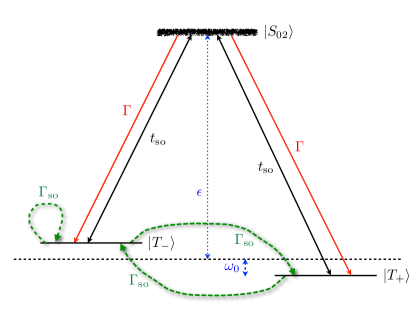
Figure 16: (color online). Phenomenological treatment of spin-orbital effects in the spin-blockade regime. Scheme of the simplified electronic system: The triplet states $\left|T_{\pm}\right\rangle$ are coherently coupled to the local singlet $\left|S_{02}\right\rangle$ by spin-orbit interaction. Via coupling to the leads, the DQD is discharged and recharged again with an effective rate $\Gamma$. The triplet states may experience a Zeeman splitting $\omega_{0}$. The parameter $\epsilon$ specifies the interdot energy offset. Since $\Gamma,\epsilon\gg t_{\mathrm{so}}$, the local singlet $\left|S_{02}\right\rangle$ can be eliminated adiabatically yielding effective dissipative processes of strength $\Gamma_{\mathrm{so}}$ (green dashed arrows).

Phenomenological treatment.—In the following, we first focus on the effects generated by $H_{\mathrm{so}}$ within the three-level subspace $\left\{\left|T_{\pm}\right\rangle,\left|S_{02}\right\rangle\right\}$. Within this reduced level scheme, the dynamics $\dot{\rho}=\mathcal{L}_{\mathrm{rd}}\rho$ are governed by the Liouvillian

$$\mathcal{L}_{\mathrm{rd}}\rho = -i\left[\mathcal{H}_{\mathrm{rd}},\rho\right]+\Gamma\sum_{\nu=\pm}\mathcal{D}\left[\left|T_{\nu}\right\rangle\left\langle S_{02}\right|\right]\rho$$ (122)

where the relevant Hamiltonian within this subspace is

$$\mathcal{H}_{\mathrm{rd}}=\omega_{0}\left(\left|T_{+}\right\rangle\left\langle T_{+}\right|-\left|T_{-}\right\rangle\left\langle T_{-}\right|\right)-\epsilon\left|S_{02}\right\rangle\left\langle S_{02}\right|+H_{\mathrm{so}}.$$ (123)

This situation is schematized in Fig. 16. The external Zeeman splitting $\omega_{0}$ is assumed to be small compared to the interdot detuning $\epsilon$ yielding approximately equal detunings between the triplet states $\left|T_{\pm}\right\rangle$ and $\left|S_{02}\right\rangle$. In particular, we consider the regime $t_{\mathrm{so}}\ll\epsilon,\Gamma$, with the corresponding separation of timescales allowing for an alternative, effective description of spin-orbital effects. Since the short-lived singlet state $\left|S_{02}\right\rangle$ is populated negligibly throughout the dynamics, it can be eliminated adiabatically using standard techniques. The symmetric superposition $\left|-\right\rangle=\left(\left|T_{+}\right\rangle-\left|T_{-}\right\rangle\right)/\sqrt{2}$ is a dark state with respect to the spin-orbit Hamiltonian $H_{\mathrm{so}}$. Therefore, it is instructive to formulate the resulting effective master equation in terms of the symmetric superposition states $\left|\pm\right\rangle=\left(\left|T_{+}\right\rangle\pm\left|T_{-}\right\rangle\right)/\sqrt{2}$. Within the two-dimensional subspace spanned by the symmetric superpositions $\left|\pm\right\rangle$, the effective dynamics is given by

$$\dot{\rho} = +i\omega_{0}\left[\left|-\right\rangle\left\langle+\right|+\left|+\right\rangle\left\langle-\right|,\rho\right]$$

$$-i\Omega_{\mathrm{so}}\left[\left|+\right\rangle\left\langle+\right|-\left|-\right\rangle\left\langle-\right|,\rho\right]$$

$$+2\Gamma_{\mathrm{so}}\mathcal{D}\left[\left|-\right\rangle\left\langle+\right|\right]\rho$$

$$+\frac{\Gamma_{\mathrm{so}}}{2}\mathcal{D}\left[\left|+\right\rangle\left\langle+\right|-\left|-\right\rangle\left\langle-\right|\right]\rho,$$

where the effective rate

$$\Gamma_{\mathrm{so}}=\frac{t_{\mathrm{so}}^{2}}{\epsilon^{2}+\Gamma^{2}}\Gamma$$ (125)

governs decay as well as pure dephasing processes within the triplet subspace. We estimate $\Gamma_{\mathrm{so}}\approx(0.2-0.3)\mu\mathrm{eV}$ which is still fast compared to typical nuclear timescales. In Eq.(D.2) we have also introduced the quantity $\Omega_{\mathrm{so}}=\left(\epsilon/\Gamma\right)\Gamma_{\mathrm{so}}$. As we are particularly concerned with the nuclear dynamics in the limit where one can eliminate the electronic degrees of freedom, Eq.(D.2) provides an alternative way of accounting for spin-orbital effects: In Eq.(D.2) we encounter a decay term—see the third line in Eq.(D.2)—which pumps the electronic subsystem towards the dark state of the spin-orbit Hamiltonian, namely the state $\left|-\right\rangle$. This state is also dark under the Stark shift and pure dephasing terms in the second and last line of Eq.(D.2), respectively. However, by applying an external magnetic field, the state $\left|-\right\rangle$ dephases due to the induced Zeeman splitting $\omega_{0}$. This becomes apparent when examining the electronic quasisteady state corresponding to the evolution given in Eq.(D.2). In the basis $\left\{\left|T_{+}\right\rangle,\mbox{$\left|T_{-}\right\rangle$}\right\}$, it is found to be

$$\rho_{\mathrm{ss}}^{\mathrm{el}}=\left(\begin{array}[]{cc}\frac{1}{2}\left[1+\frac{\omega_{0}\Omega_{\mathrm{so}}}{\omega_{0}^{2}+\Gamma_{\mathrm{so}}^{2}+\Omega_{\mathrm{so}}^{2}}\right]&-\frac{\Gamma_{\mathrm{so}}^{2}+\Omega_{\mathrm{so}}^{2}+i\Gamma_{\mathrm{so}}\omega_{0}}{2\left(\omega_{0}^{2}+\Gamma_{\mathrm{so}}^{2}+\Omega_{\mathrm{so}}^{2}\right)}\\ -\frac{\Gamma_{\mathrm{so}}^{2}+\Omega_{\mathrm{so}}^{2}-i\Gamma_{\mathrm{so}}\omega_{0}}{2\left(\omega_{0}^{2}+\Gamma_{\mathrm{so}}^{2}+\Omega_{\mathrm{so}}^{2}\right)}&\frac{1}{2}\left[1-\frac{\omega_{0}\Omega_{\mathrm{so}}}{\omega_{0}^{2}+\Gamma_{\mathrm{so}}^{2}+\Omega_{\mathrm{so}}^{2}}\right]\end{array}\right),$$ (126)

which in leading orders of $\omega_{0}^{-1}$ reduces to

$$\rho_{\mathrm{ss}}^{\mathrm{el}}\approx\left(\begin{array}[]{cc}\frac{1}{2}+\frac{\Omega_{\mathrm{so}}}{2\omega_{0}}&-i\frac{\Gamma_{\mathrm{so}}}{2\omega_{0}}\\ i\frac{\Gamma_{\mathrm{so}}}{2\omega_{0}}&\frac{1}{2}-\frac{\Omega_{\mathrm{so}}}{2\omega_{0}}\end{array}\right).$$ (127)

Accordingly, for sufficiently large Zeeman splitting $\omega_{0}\gg\Omega_{\mathrm{so}},\Gamma_{\mathrm{so}}$, the electronic subsystem is driven towards the desired equal mixture of blocked triplet states $\left|T_{+}\right\rangle$ and $\left|T_{-}\right\rangle$. Alternatively, the off-diagonal elements of $\left|-\right\rangle\left\langle-\right|$ are damped out in the presence of dephasing processes either mediated intrinsically via cotunneling processes or extrinsically via engineered magnetic noise yielding approximately the equal mixture $\rho_{\mathrm{target}}^{\mathrm{el}}=\left(\left|T_{+}\right\rangle\left\langle T_{+}\right|+\left|T_{-}\right\rangle\left\langle T_{-}\right|\right)/2$ in the quasisteady state.

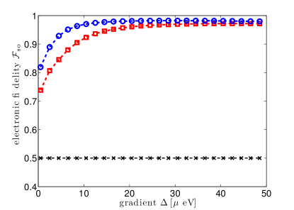
Figure 17: (color online). Electronic quasi-steady-state fidelities in the presence of spin-orbit coupling for the dynamics generated by $\tilde{\mathcal{K}}_{0}$ as a function of the gradient $\Delta$. As expected, in the absence of dephasing [$\Gamma_{\mathrm{deph}}=0$ (black curve)], the system settles into the dark state $\left|-\right\rangle$. For $\Gamma_{\mathrm{deph}}=1\mu\mathrm{eV}$ (blue and red curves), the off-diagonal elements of $\left|-\right\rangle$ are strongly suppressed, leading to a high fidelity $\mathcal{F}_{\mathrm{so}}\gtrsim 0.9$ with the desired mixed state $\rho_{\mathrm{target}}^{\mathrm{el}}$ in the high gradient regime: the blue and red curve refer to $t=20\mu\mathrm{eV}$ and $t=30\mu\mathrm{eV}$, respectively. Other numerical parameters are: $t_{\mathrm{so}}=0.1t$, $\omega_{0}=0$, $\Gamma=25\mu\mathrm{eV}$ and $\epsilon=30\mu\mathrm{eV}$.

Numerical analysis.—To complement the perturbative, analytical study, we carry out a numerical evaluation of the electronic quasisteady state in the presence of spin-orbit coupling. In the two-electron subspace, the corresponding master equation (including spin-orbital effects) under consideration reads

$$\dot{\rho}=\tilde{\mathcal{K}}_{0}\rho=-i\left[H_{\mathrm{el}}+H_{\mathrm{so}},\rho\right]+\mathcal{K}_{\Gamma}\rho+\mathcal{L}_{\mathrm{deph}}\rho.$$ (128)

We evaluate the exact electronic quasisteady state $\rho_{\mathrm{ss}}^{\mathrm{el}}$ fulfilling $\tilde{\mathcal{K}}_{0}\rho_{\mathrm{ss}}^{\mathrm{el}}=0$. As a figure of merit, we compute the Uhlmann fidelity uhlmann76

$$\mathcal{F}_{\text{$\mathrm{so}$}}=\mathrm{tr}\left[\left(\sqrt{\rho_{\mathrm{ss}}^{\mathrm{el}}}\rho_{\mathrm{target}}^{\mathrm{el}}\sqrt{\rho_{\mathrm{ss}}^{\mathrm{el}}}\right)^{1/2}\right]^{2}$$ (129)

which measures how similar $\rho_{\mathrm{ss}}^{\mathrm{el}}$ and $\rho_{\mathrm{target}}^{\mathrm{el}}$ are. The results are illustrated in Fig. 17: For $\Gamma_{\mathrm{deph}}=0$ the electronic system settles into the pure dark state $\left|-\right\rangle\left\langle-\right|$. However, in the presence of dephasing, the coherences are efficiently damped out. In the low-gradient regime $\rho_{\mathrm{ss}}^{\mathrm{el}}$ has a significant overlap with the triplet $\left|T_{0}\right\rangle$, whereas in the high-gradient regime it is indeed approximately given by the desired mixed target state $\rho_{\mathrm{target}}^{\mathrm{el}}$. Lastly, we have checked that in the high-gradient regime the corresponding asymptotic decay rate can be approximated very well by $\mathrm{ADR}_{\mathrm{el}}\approx-2\Gamma_{\mathrm{so}}$.

Appendix E Effective Nuclear Master Equation

In this appendix, we present a detailed derivation of the effective nuclear dynamics presented in Section III. We use standard adiabatic elimination techniques to derive an effective simplified description of the dynamics. To do so, we assume that electronic coherences decay quickly on typical nuclear timescales. Conservatively, i.e. not taking into account the detuning of the HF-mediated transitions, this holds for $2\Gamma_{\pm}+\Gamma_{\mathrm{deph}}/4\gg g_{\mathrm{hf}}$, where $g_{\mathrm{hf}}$ quantifies the typical HF interaction strength. Alternatively, one may use a projection-operator based technique;schuetz12 ; kessler12 this is done in detail in Appendix H for the high-gradient regime where $\rho_{\mathrm{ss}}^{\mathrm{el}}=\left(\left|T_{+}\right\rangle\left\langle T_{+}\right|+\left|T_{-}\right\rangle\left\langle T_{-}\right|\right)/2$, but a generalization for the electronic quasisteady state in Eq.(33) is straightforward.

Throughout this appendix, for convenience we adopt the following notation: $\left|a\right\rangle=\left|T_{+}\right\rangle$, $\left|b\right\rangle=\left|\lambda_{2}\right\rangle$, $\left|c\right\rangle=\left|T_{-}\right\rangle$, $L=L_{2}$, $\mathbb{L}=\mathbb{L}_{2}$ and $\mathcal{D}\left[c\right]\rho=\mathcal{D}_{c}\rho$. Within this simplified three-level model system, the flip-flop Hamiltonian $H_{\mathrm{ff}}$ reads

$$H_{\mathrm{ff}}=\frac{a_{\mathrm{hf}}}{2}\left[L\left|b\right\rangle\left\langle a\right|+\mathbb{L}\left|b\right\rangle\left\langle c\right|+\mathrm{h.c.}\right].$$ (130)

For simplicity, we assume $\omega_{0}=0$ and neglect nuclear fluctuations arising from $H_{\mathrm{zz}}$. This approximation is in line with the semiclassical approximation for studying the nuclear polarization dynamics; for more details also see Appendix F. Within this reduced scheme, the dynamics are then described by the Master equation

$$\dot{\rho} = -i\left[H_{\mathrm{ff}},\rho\right]-i\epsilon_{2}\left[\left|b\right\rangle\left\langle b\right|,\rho\right]+\frac{\Gamma_{\mathrm{deph}}}{2}\mathcal{D}_{\left|a\right\rangle\left\langle a\right|-\left|c\right\rangle\left\langle c\right|}\rho$$ (131)

$$+\Gamma_{\pm}\left[\mathcal{D}_{\left|c\right\rangle\left\langle a\right|}\rho+\mathcal{D}_{\left|a\right\rangle\left\langle c\right|}\rho+\mathcal{D}_{\left|b\right\rangle\left\langle a\right|}\rho+\mathcal{D}_{\left|b\right\rangle\left\langle c\right|}\rho\right]$$

$$+\left(\Gamma_{\pm}+\Gamma_{2}\right)\left[\mathcal{D}_{\left|a\right\rangle\left\langle b\right|}\rho+\mathcal{D}_{\left|c\right\rangle\left\langle b\right|}\rho\right].$$

After adiabatic elimination of the electronic coherences $\rho_{ab}=\left<a|\rho|b\right>$, $\rho_{cb}$ and $\rho_{ac}$ we obtain effective equations of motion for the system’s density matrix projected onto the electronic levels $\left|a\right\rangle$, $\left|b\right\rangle$ and $\left|c\right\rangle$ as follows

$$\dot{\rho}_{aa} = \Gamma_{\pm}\left(\rho_{cc}-\rho_{aa}\right)+\Gamma_{\pm}\left(\rho_{bb}-\rho_{aa}\right)+\Gamma_{2}\rho_{bb}$$

$$+\gamma\left[L^{\dagger}\rho_{bb}L-\frac{1}{2}\left\{L^{\dagger}L,\rho_{aa}\right\}\right]$$

$$+i\delta\left[L^{\dagger}L,\rho_{aa}\right],$$

$$\dot{\rho}_{cc} = \Gamma_{\pm}\left(\rho_{aa}-\rho_{cc}\right)+\Gamma_{\pm}\left(\rho_{bb}-\rho_{cc}\right)+\Gamma_{2}\rho_{bb}$$

$$+\gamma\left[\mathbb{L}^{\dagger}\rho_{bb}\mathbb{L}-\frac{1}{2}\left\{\mathbb{L}^{\dagger}\mathbb{L},\rho_{cc}\right\}\right]$$

$$+i\delta\left[\mathbb{L}^{\dagger}\mathbb{L},\rho_{cc}\right],$$

and

$$\dot{\rho}_{bb} = -2\Gamma_{2}\rho_{bb}+\gamma\left[L\rho_{aa}L^{\dagger}-\frac{1}{2}\left\{LL^{\dagger},\rho_{bb}\right\}\right]$$

$$-i\delta\left[LL^{\dagger},\rho_{bb}\right]$$

$$+\gamma\left[\mathbb{L}\rho_{cc}\mathbb{L^{\dagger}}-\frac{1}{2}\left\{\mathbb{L}\mathbb{L^{\dagger}},\rho_{bb}\right\}\right]-i\delta\left[\mathbb{L}\mathbb{L^{\dagger}},\rho_{bb}\right].$$

$$+\Gamma_{\pm}\left(\rho_{aa}+\rho_{cc}-2\rho_{bb}\right).$$

Since this set of equations is entirely expressed in terms of $\rho_{aa}$, $\rho_{bb}$ and $\rho_{cc}$, the full density matrix of the system obeys a simple block structure, given by

$$\rho=\rho_{aa}\left|a\right\rangle\left\langle a\right|+\rho_{bb}\left|b\right\rangle\left\langle b\right|+\rho_{cc}\left|c\right\rangle\left\langle c\right|.$$ (135)

Therefore, the electronic decoherence is fast enough to prevent the entanglement between electronic and nuclear degrees of freedom and the total density matrix of the system $\rho$ factorizes into a tensor product for the electronic and nuclear subsystem,rudner07b respectively, that is $\rho=\rho_{\mathrm{el}}\otimes\sigma,$ where $\sigma=\mathsf{Tr}_{\mathrm{el}}\left[\rho\right]$ refers to the density matrix of the nuclear subsystem. This ansatz agrees with the projection operator approach where $\mathcal{P}\rho=\sigma\otimes\rho_{\mathrm{el}}$ and readily yields $\rho_{aa}=p_{a}\sigma$, where we have introduced the electronic populations

$$p_{a}=\left<a|\rho_{\mathrm{el}}|a\right>=\mathsf{Tr}_{\mathrm{n}}\left[\rho_{aa}\right],$$ (136)

and accordingly for $p_{b}$ and $p_{c}$; here, $\mathsf{Tr}_{\mathrm{n}}\left[\dots\right]$ denotes the trace over the nuclear degrees of freedom. With these definitions, Eqs. (E), (E) and (E) can be rewritten as

$$\dot{p}_{a} = \Gamma_{\pm}\left(p_{c}-p_{a}\right)+\Gamma_{2}p_{b}+\gamma\left[p_{b}\left\langle LL^{\dagger}\right\rangle-p_{a}\left\langle L^{\dagger}L\right\rangle\right]$$

$$+\Gamma_{\pm}\left(p_{b}-p_{a}\right),$$

$$\dot{p}_{c} = \Gamma_{\pm}\left(p_{a}-p_{c}\right)+\Gamma_{2}p_{b}+\gamma\left[p_{b}\left\langle\mathbb{L}\mathbb{L}^{\dagger}\right\rangle-p_{c}\left\langle\mathbb{L}^{\dagger}\mathbb{L}\right\rangle\right]$$

$$+\Gamma_{\pm}\left(p_{b}-p_{c}\right),$$

$$\dot{p}_{b} = -2\Gamma_{2}p_{b}+\Gamma_{\pm}\left(p_{a}+p_{c}-2p_{b}\right)$$ (137)

$$+\gamma\left[p_{a}\left\langle L^{\dagger}L\right\rangle-p_{b}\left\langle LL^{\dagger}\right\rangle+p_{c}\left\langle\mathbb{L}^{\dagger}\mathbb{L}\right\rangle-p_{b}\left\langle\mathbb{L}\mathbb{L}^{\dagger}\right\rangle\right].$$

Similarly, the effective Master equation for the nuclear density matrix $\sigma=\mathsf{Tr}_{\mathrm{el}}\left[\rho\right]$ is obtained from $\dot{\sigma}=\mathsf{Tr}_{\mathrm{el}}\left[\dot{\rho}\right]=\dot{\rho}_{aa}+\dot{\rho}_{bb}+\dot{\rho}_{cc}$, leading to

$$\dot{\sigma} = \gamma\left\{p_{b}\mathcal{D}_{L^{\dagger}}\left[\text{$\sigma$}\right]+p_{b}\mathcal{D}_{\mathbb{L}^{\dagger}}\left[\sigma\right]+p_{a}\mathcal{D}_{L}\left[\sigma\right]+p_{c}\mathcal{D}_{\mathbb{L}}\left[\sigma\right]\right\}$$ (138)

$$+i\delta\left\{p_{a}\left[L^{\dagger}L,\sigma\right]+p_{c}\left[\mathbb{L}^{\dagger}\mathbb{L},\sigma\right]\right.$$

$$\left.-p_{b}\left[LL^{\dagger},\sigma\right]-p_{b}\left[\mathbb{L}\mathbb{L}^{\dagger},\sigma\right]\right\}.$$

Equation (138) along with Eq.(137) describe the coupled electron-nuclear dynamics on a coarse-grained timescale that is long compared to electronic coherence timescales. Due to the normalization condition $p_{a}+p_{b}+p_{c}=1$, this set of dynamical equations comprises three coupled equations. Differences in the populations of the levels $\left|a\right\rangle$ and $\left|c\right\rangle$ decay very quickly on timescales relevant for the nuclear evolution; that is,

$$\dot{p}_{a}-\dot{p}_{c} = -3\Gamma_{\pm}\left(p_{a}-p_{c}\right)+\gamma\left[p_{b}\left(\left\langle LL^{\dagger}\right\rangle-\left\langle\mathbb{L}\mathbb{L}^{\dagger}\right\rangle\right)\right.$$ (139)

$$\left.-p_{a}\left\langle L^{\dagger}L\right\rangle+p_{c}\left\langle\mathbb{L}^{\dagger}\mathbb{L}\right\rangle\right]$$

Due to a separation of timescales, as $\Gamma_{\pm}\gg\gamma_{c}=N\gamma\approx 10^{-4}\mu\mathrm{eV}$, in a perturbative treatment the effect of the second term can be neglected and the electronic subsystem approximately settles into $p_{a}=p_{c}$. This leaves us with a single dynamical variable, namely $p_{a}$, entirely describing the electronic subsystem on relevant timescales. Thus, using $p_{c}=p_{a}$ and $p_{b}=1-2p_{a}$, the electronic quasi steady state is uniquely defined by the parameter $p_{a}$ and the nuclear evolution simplifies to

$$\dot{\sigma} = \gamma\left\{p_{a}\left[\mathcal{D}_{L}\left[\sigma\right]+\mathcal{D}_{\mathbb{L}}\left[\sigma\right]\right]\right.$$

$$\left.+\left(1-2p_{a}\right)\left[\mathcal{D}_{L^{\dagger}}\left[\sigma\right]+\mathcal{D}_{\mathbb{L}^{\dagger}}\left[\sigma\right]\right]\right\}$$

$$+i\delta\left\{p_{a}\left(\left[L^{\dagger}L,\sigma\right]+\left[\mathbb{L}^{\dagger}\mathbb{L},\sigma\right]\right)\right.$$

$$\left.-\left(1-2p_{a}\right)\left(\left[LL^{\dagger},\sigma\right]+\left[\mathbb{L}\mathbb{L}^{\dagger},\sigma\right]\right)\right\},$$

with $p_{a}$ obeying the dynamical equation

$$\dot{p}_{a} = \Gamma_{\pm}\left(1-3p_{a}\right)+\Gamma_{2}\left(1-2p_{a}\right)$$

$$-\gamma\left[p_{a}\left\langle L^{\dagger}L\right\rangle+\left(1-2p_{a}\right)\left\langle LL^{\dagger}\right\rangle\right].$$

Neglecting the HF terms in the second line, we recover the projection-operator-based result for the quasisteady state, $p_{a}\approx\left(\Gamma_{\pm}+\Gamma_{2}\right)/\left(3\Gamma_{\pm}+2\Gamma_{2}\right)$ as stated in Eq.(34).

Appendix F Effective Nuclear Dynamics: Overhauser Fluctuations

In Sec. III we have disregarded the effect of Overhauser fluctuations, described by $\dot{\rho}=-i\left[H_{\mathrm{zz}},\rho\right]=-ia_{\mathrm{hf}}\sum_{i}\left[S_{i}^{z}\delta A_{i}^{z},\rho\right].$ In the following analysis, this simplification is discussed in greater detail.

First of all, we note that this term cannot induce couplings within the effective electronic three level system, $\left\{\left|T_{\pm}\right\rangle,\left|\lambda_{2}\right\rangle\right\}$, since $\left|T_{\pm}\right\rangle$ are eigenstates of $S_{i}^{z}$, that is explicitly $S_{i}^{z}\left|T_{\pm}\right\rangle=\pm\frac{1}{2}\left|T_{\pm}\right\rangle$, which leads to

$$\left<T_{\pm}|S_{i}^{z}|\lambda_{2}\right>=0.$$ (141)

In other words, different $S_{\mathrm{tot}}^{z}$ subspaces are not coupled by the action of $H_{\mathrm{zz}}$; this is in stark contrast to the flip flop dynamics $H_{\mathrm{ff}}$.

When also accounting for Overhauser fluctuations, the dynamical equations for the coherences read

$$\dot{\rho}_{ab} = \left(i\epsilon_{2}-\tilde{\Gamma}\right)\rho_{ab}-i\left[L^{\dagger}\rho_{bb}-\rho_{aa}L^{\dagger}\right]$$

$$-ia_{\mathrm{hf}}\sum_{i}\left[\left\langle S_{i}^{z}\right\rangle_{a}\delta A_{i}^{z}\rho_{ab}-\left\langle S_{i}^{z}\right\rangle_{b}\rho_{ab}\delta A_{i}^{z}\right],$$

where $\left\langle S_{i}^{z}\right\rangle_{a}=\left<a|S_{i}^{z}|a\right>$; an analog equation holds for $\dot{\rho}_{cb}$. Typically, the second line is small compared to the fast electronic quantities $\epsilon_{2},\tilde{\Gamma}$ in the first line. Therefore, it will be neglected. In Eqs.(E), (E) and(E), the Overhauser fluctuations lead to the following additional terms

$$\dot{\rho}_{aa} = \dots-\frac{i}{2}a_{\mathrm{hf}}\sum_{i}\left[\delta A_{i}^{z},\rho_{aa}\right],$$ (143)

$$\dot{\rho}_{cc} = \dots+\frac{i}{2}a_{\mathrm{hf}}\sum_{i}\left[\delta A_{i}^{z},\rho_{cc}\right],$$ (144)

$$\dot{\rho}_{bb} = \dots-ia_{\mathrm{hf}}\sum_{i}\left\langle S_{i}^{z}\right\rangle_{b}\left[\delta A_{i}^{z},\rho_{bb}\right].$$ (145)

First, this leaves the electronic populations $p_{a}=\mathsf{Tr}_{\mathrm{n}}\left[\rho_{aa}\right]$ untouched; $H_{\mathrm{zz}}$ does not induce any couplings between them. Second, the dynamical equation for the nuclear density matrix $\sigma=\mathsf{Tr}_{\mathrm{el}}\left[\rho\right]$ is modified as

$$\dot{\sigma} = \dots-ia_{\mathrm{hf}}\sum_{i}\left[\frac{1}{2}\left(p_{a}-p_{c}\right)+p_{b}\left\langle S_{i}^{z}\right\rangle_{b}\right]\left[\delta A_{i}^{z},\sigma\right],$$ (146)

$$\approx \dots-i\left(1-2p_{a}\right)a_{\mathrm{hf}}\sum_{i}\left\langle S_{i}^{z}\right\rangle_{b}\left[\delta A_{i}^{z},\sigma\right].$$

In the second step, we have used again that differences in $p_{a}$ and $p_{c}$ are quickly damped to zero with a rate of $3\Gamma_{\pm}$. Now, let us examine the effect of Eq.(146) for different important regimes: In the high gradient regime, where $p_{b}$ is fully depleted, it does not give any contribution since the electronic quasi steady state does not have any magnetization $\left[\left\langle S_{i}^{z}\right\rangle_{b}=\left\langle S_{i}^{z}\right\rangle_{\mathrm{ss}}=0\right]$ and $p_{a}=1/2$. In the low gradient regime, $\left|b\right\rangle$ approaches the triplet $\left|T_{0}\right\rangle$ and again (since $\left\langle S_{i}^{z}\right\rangle_{b}=0$) this term vanishes. Finally, the intermediate regime has been studied within a semiclassical approximation (see section IV): Note that Eq.(146), however, leaves the dynamical equation for the nuclear polarizations $I_{i}^{z}$ unchanged, since they commute with $H_{\mathrm{zz}}$.

Appendix G Numerical Results for DNP

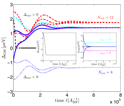
Figure 18: (color online). Exact time evolution for $N=8$ and $N=12$ (red dashed curves) nuclear spins, four and six in each quantum dot, respectively. Depending on the initial value of the gradient, the nuclear system either runs into the trivial, unpolarized state or into the highly polarized one, if the initial gradient exceeds the critical value; the blue dotted, black dash-dotted and all other refer to $\Delta_{\mathrm{ext}}=-5\mu\mathrm{eV}$, $\Delta_{\mathrm{ext}}=0$ and $\Delta_{\mathrm{ext}}=5\mu\mathrm{eV}$, respectively. For $\omega_{\mathrm{ext}}\neq 0$, also a homogeneous OH field $\omega_{\mathrm{OH}}$ builds up which partially compensates $\omega_{\mathrm{ext}}$: here, $\omega_{\mathrm{ext}}=0.1\mu\mathrm{eV}$ (magenta dash-dotted) and $\omega_{\mathrm{ext}}=-0.1\mu\mathrm{eV}$ (cyan dash-dotted). Other numerical parameters: $t=10\mu\mathrm{eV}$, $\epsilon=30\mu\mathrm{eV}$, $\Gamma=25\mu\mathrm{eV}$, $\Gamma_{\pm}=\Gamma_{\mathrm{deph}}=0.1\mu\mathrm{eV}$.

In this appendix the analytical findings of the semiclassical model are corroborated by exact numerical simulations for small sets of nuclear spins. This treatment complements our analytical DNP analysis in several aspects: First, we do not restrict ourselves to the effective three level system $\left\{\left|T_{\pm}\right\rangle,\left|\lambda_{2}\right\rangle\right\}$. Second, the electronic degrees of freedom are not eliminated adiabatically from the dynamics. Lastly, this approach does not involve the semiclassical decorrelation approximation stated in Eq.(46).

Technical details.—We consider the idealized case of homogeneous hyperfine coupling for which an exact numerical treatment is feasible even for a relatively large number of coupled nuclei as the system evolves within the totally symmetric low-dimensional subspace $\left\{\left|J,m\right\rangle,m=-J,\dots,J\right\}$, referred to as Dicke ladder. We restrict ourselves to the fully symmetric subspace where $J_{i}=N_{i}/2\approx 3$. Moreover, to mimic the separation of timescales in experiments where $N\approx 10^{6}$, the HF coupling is scaled down appropriately to the constant value $g_{\mathrm{hf}}\approx 0.1\mu\mathrm{eV}$; also compare the numerical results presented in Fig. 6.

Our first numerical approach is based on simulations of the time evolution. Starting out from nuclear states with different initial Overhauser gradient $\Delta_{\mathrm{OH}}\left(t=0\right)$, we make the following observations, depicted in Fig. 18: First of all, the tri-stability of the Overhauser gradient with respect to the initial nuclear polarization is confirmed. If the initial gradient $\Delta_{\mathrm{OH}}\left(t=0\right)+\Delta_{\mathrm{ext}}$ exceeds a certain threshold value, the nuclear system runs into the highly-polarized steady state, otherwise it gets stuck in the trivial, zero-polarization solution. There are two symmetric high-polarization solutions that depend on the sign of $\Delta_{\mathrm{OH}}\left(t=0\right)+\Delta_{\mathrm{ext}}$; also note that the Overhauser gradient $\Delta_{\mathrm{OH}}$ may flip the sign as determined by the total initial gradient $\Delta_{\mathrm{OH}}\left(t=0\right)+\Delta_{\mathrm{ext}}$. Second, in the absence of an external Zeeman splitting $\omega_{\mathrm{ext}}$, a potential initial homogeneous Overhauser polarizations $\bar{\omega}_{\mathrm{OH}}$ is damped to zero in the steady state. For finite $\omega_{\mathrm{ext}}\neq 0$, a homogeneous Overhauser polarization $\bar{\omega}_{\mathrm{OH}}$ builds up which partially compensates $\omega_{\mathrm{ext}}$. Lastly, the high-polarization solutions $\Delta_{\mathrm{OH}}^{\mathrm{ss}}\approx 2\mu\mathrm{eV}$ are far away from full polarization. This is an artifact of the small system sizes $J_{i}\approx 3$: As we deal with very short Dicke ladders, even the ideal, nuclear two-mode squeezedlike target state $\left|\xi\right\rangle_{\mathrm{ss}}$ given in Eq.(7) does not feature a very high polarization. Pictorially, it leaks with a non-vanishing factor $\sim\xi^{m}$ into the low-polarization Dicke states. This argument is supported by the fact that (for the same set of parameters) we observe tendency towards higher polarization for an increasing number of nuclei $N$ (which features a larger Dicke ladder) and confirmed by our second numerical approach to be discussed below.

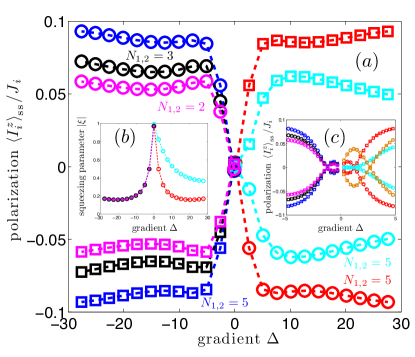
Figure 19: (color online). Instability towards nuclear self-polarization: Exact numerical results for small system sizes $J_{i}=N_{i}/2$. The exact steady state of the coupled electron-nuclear dynamics is computed as a function of the gradient $\Delta$. The circles (squares) refer to the polarization in the left (right) dot, respectively. (a) For $\Delta>\left|\Delta_{\mathrm{OH}}^{\mathrm{crt}}\right|$, we find $\Delta_{\mathrm{OH}}>0$, whereas for $\Delta<-\left|\Delta_{\mathrm{OH}}^{\mathrm{crt}}\right|$ we get $\Delta_{\mathrm{OH}}<0$, i.e., outside of the small-gradient regime [see inset (c)] the nuclear system is seen to be unstable towards the buildup of a OH gradient with opposite polarizations in the two dots. The nuclear polarization depends on the system size $J_{i}$ and the parameter $\left|\xi\right|$; compare inset (b). (c) The critical value of $\Delta_{\mathrm{OH}}^{\mathrm{crt}}\approx 3\mu\mathrm{eV}$ agrees with the semiclassical estimate; it becomes smaller for smaller values of $\Gamma_{\pm}$. Numerical parameters in $\mu\mathrm{eV}$: $\epsilon=30$, $\Gamma=10$, $\Gamma_{\pm}=\Gamma_{\mathrm{deph}}=0.3$, $\omega_{\mathrm{ext}}=0$ and $t=10$ except for the cyan curve where $t=20$ and $\Gamma_{\pm}=\Gamma_{\mathrm{deph}}=0.6$ for the orange curve in (c).

Our second numerical approach is based on exact diagonalization: As we tune the parameter $\Delta$, we compute the steady state for the full electronic-nuclear system directly giving the corresponding steady-state nuclear polarizations $\left\langle I_{i}^{z}\right\rangle_{\mathrm{ss}}$. We see a clear instability towards the buildup of an Overhauser gradient $\Delta_{\mathrm{OH}}^{\mathrm{ss}}$ (Fig. 19): Inside the small-gradient region $\left(\left|\Delta\right|<\left|\Delta_{\mathrm{OH}}^{\mathrm{crt}}\right|\right)$ we observe negative feedback $\mathrm{sgn}\left(\Delta_{\mathrm{OH}}^{\mathrm{ss}}\right)=-\mathrm{sgn}\left(\Delta\right)$, whereas outside of it $\left(\left|\Delta\right|>\left|\Delta_{\mathrm{OH}}^{\mathrm{crt}}\right|\right)$ the nuclear system experiences positive feedback $\mathrm{sgn}\left(\Delta_{\mathrm{OH}}^{\mathrm{ss}}\right)=\mathrm{sgn}\left(\Delta\right)$. The latter leads to the build-up of large OH gradients, in agreement with our semiclassical analysis.

Appendix H Effective Nuclear Master Equation in High-Gradient Regime

This Appendix provides background material for the derivation of the effective nuclear master equation as stated in Eq.(55) using projection-operator techniqueskessler12 ; schuetz12 . We start with

$$\mathsf{Tr}_{\mathrm{el}}\left[\mathcal{P}\mathcal{V}\mathcal{P}\rho\right]=\mathsf{Tr}_{\mathrm{el}}\left[\mathcal{P}\mathcal{L}_{\mathrm{ff}}\mathcal{P}\rho\right]+\mathsf{Tr}_{\mathrm{el}}\left[\mathcal{P}\mathcal{L}_{\mathrm{zz}}\mathcal{P}\rho\right]$$ (147)

The first term is readily found to be

$$\mathsf{Tr}_{\mathrm{el}}\left[\mathcal{P}\mathcal{L}_{\mathrm{ff}}\mathcal{P}\rho\right]=-i\frac{a_{\mathrm{hf}}}{2}\sum_{i,\alpha=\pm}\left\langle S_{i}^{\alpha}\right\rangle_{\mathrm{ss}}\left[A_{i}^{\bar{\alpha}},\sigma\right],$$ (148)

where $\left\langle\cdot\right\rangle_{\mathrm{ss}}=\mathsf{Tr}_{\mathrm{el}}\left[\cdot\rho_{\mathrm{ss}}^{\mathrm{el}}\right]$ denotes the steady-state expectation value. An analog calculation yields

$$\mathsf{Tr}_{\mathrm{el}}\left[\mathcal{P}\mathcal{L}_{\mathrm{zz}}\mathcal{P}\rho\right]=-ia_{\mathrm{hf}}\sum_{i}\left\langle S_{i}^{z}\right\rangle_{\mathrm{ss}}\left[\delta A_{i}^{z},\sigma\right].$$ (149)

Using that $\left\langle S_{i}^{\alpha}\right\rangle_{\mathrm{ss}}=0$ and $\left\langle S_{i}^{z}\right\rangle_{\mathrm{ss}}=0$ [the Knight shift seen by the nuclear spins is zero since the electronic quasi steady-state carries no net magnetization], the first two Hamiltonian terms vanish.

The second-order term of interest

$$\mathcal{K}\sigma=\mathsf{Tr}_{\mathrm{el}}\left[\mathcal{P}\mathcal{V}\mathcal{Q}\left(-\mathcal{L}_{0}^{-1}\right)\mathcal{Q}\mathcal{V}\mathcal{P}\rho\right]$$ (150)

can be decomposed as $\mathcal{K}\sigma=\mathcal{K}_{\mathrm{ff}}\sigma+\mathcal{K}_{\mathrm{zz}}\sigma$, where

$$\mathcal{K}_{\mathrm{ff}}\sigma = \mathsf{Tr}_{\mathrm{el}}\left[\mathcal{P}\mathcal{L}_{\mathrm{ff}}\mathcal{Q}\left(-\mathcal{L}_{0}^{-1}\right)\mathcal{Q}\mathcal{L}_{\mathrm{ff}}\mathcal{P}\rho\right],$$ (151)

$$\mathcal{K}_{\mathrm{zz}}\sigma = \mathsf{Tr}_{\mathrm{el}}\left[\mathcal{P}\mathcal{L}_{\mathrm{zz}}\mathcal{Q}\left(-\mathcal{L}_{0}^{-1}\right)\mathcal{Q}\mathcal{L}_{\mathrm{zz}}\mathcal{P}\rho\right].$$ (152)

All other second order terms containing combinations of the superoperators $\mathcal{L}_{\mathrm{ff}}$ and $\mathcal{L}_{\mathrm{zz}}$ can be shown to vanish. In the following, we will evaluate the two terms separately.

Hyperfine flip-flop dynamics.—First, we will evaluate $\mathcal{K}_{\mathrm{ff}}$ which can be rewritten as

$$\mathcal{K}_{\mathrm{ff}}\sigma = \underset{\leavevmode\hbox to12.65pt{\vbox to12.65pt{\text{[drawing]}}}}{\underbrace{\int_{0}^{\infty}d\tau\mathsf{Tr}_{\mathrm{el}}\left[\mathcal{P}\mathcal{L}_{\mathrm{ff}}e^{\mathcal{L}_{0}\tau}\mathcal{L}_{\mathrm{ff}}\mathcal{P}\rho\right]}}$$ (153)

$$\underset{\leavevmode\hbox to14.92pt{\vbox to14.92pt{\text{[drawing]}}}}{\underbrace{-\int_{0}^{\infty}d\tau\mathsf{Tr}_{\mathrm{el}}\left[\mathcal{P}\mathcal{L}_{\mathrm{ff}}\mathcal{P}\mathcal{L}_{\mathrm{ff}}\mathcal{P}\rho\right]}}.$$

Here, we used the Laplace transform $-\mathcal{L}_{0}^{-1}=\int_{0}^{\infty}d\tau e^{\mathcal{L}_{0}\tau}$ and the property $e^{\mathcal{L}_{0}\tau}\mathcal{P}=\mathcal{P}e^{\mathcal{L}_{0}\tau}=\mathcal{P}$.kessler12 The first term labeled as is given by

$$\leavevmode\hbox to12.65pt{\vbox to12.65pt{\text{[drawing]}}}=-\int_{0}^{\infty}d\tau\mathsf{Tr}_{\mathrm{el}}\left(\left[H_{\mathrm{ff}},e^{\mathcal{L}_{0}\tau}\left[H_{\mathrm{ff}},\sigma\otimes\rho_{\mathrm{ss}}^{\mathrm{el}}\right]\right]\right).$$ (154)

Then, using the relations

$$\mathcal{L}_{0}\left[\left|\lambda_{k}\right\rangle\left\langle T_{\pm}\right|\right] = -i\left(\delta_{k}^{\pm}-i\tilde{\Gamma}_{k}\right)\left|\lambda_{k}\right\rangle\left\langle T_{\pm}\right|,$$ (155)

$$\mathcal{L}_{0}\left[\left|T_{\pm}\right\rangle\left\langle\lambda_{k}\right|\right] = +i\left(\delta_{k}^{\pm}+i\tilde{\Gamma}_{k}\right)\left|T_{\pm}\right\rangle\left\langle\lambda_{k}\right|,$$ (156)

where (to shorten the notation) $\delta_{k}^{+}=\Delta_{k}$ and $\delta_{k}^{-}=\delta_{k}$, respectively, we find

$$e^{\mathcal{L}_{0}\tau}\left(H_{\mathrm{ff}}\sigma\rho_{\mathrm{ss}}^{\mathrm{el}}\right) = \frac{a_{\mathrm{hf}}}{4}\sum_{k}\left[e^{-i\left(\delta_{k}^{+}-i\tilde{\Gamma}_{k}\right)\tau}\left|\lambda_{k}\right\rangle\left\langle T_{+}\right|L_{k}\sigma\right.$$ (157)

$$\left.+e^{-i\left(\delta_{k}^{-}-i\tilde{\Gamma}_{k}\right)\tau}\left|\lambda_{k}\right\rangle\left\langle T_{-}\right|\mathbb{L}_{k}\sigma\right],$$

and along the same lines

$$e^{\mathcal{L}_{0}\tau}\left(\sigma\rho_{\mathrm{ss}}^{\mathrm{el}}H_{\mathrm{ff}}\right) = \frac{a_{\mathrm{hf}}}{4}\sum_{k}\left[e^{+i\left(\delta_{k}^{+}+i\tilde{\Gamma}_{k}\right)\tau}\left|T_{+}\right\rangle\left\langle\lambda_{k}\right|\sigma L_{k}^{\dagger}\right.$$ (158)

$$\left.+e^{+i\left(\delta_{k}^{-}+i\tilde{\Gamma}_{k}\right)\tau}\left|T_{-}\right\rangle\left\langle\lambda_{k}\right|\sigma\mathbb{L}_{k}^{\dagger}\right].$$

Plugging Eq.(157) and Eq.(158) into Eq.(154), tracing out the electronic degrees of freedom, performing the integration in $\tau$ and separating real and imaginary parts of the complex eigenvalues leads to

$$= \sum_{k}\left[\frac{\gamma_{k}^{+}}{2}\mathcal{D}\left[L_{k}\right]\sigma+i\frac{\Delta_{k}^{+}}{2}\left[L_{k}^{\dagger}L_{k},\sigma\right]\right.$$ (160)

$$\left.+\frac{\gamma_{k}^{-}}{2}\mathcal{D}\left[\mathbb{L}_{k}\right]\sigma+i\frac{\Delta_{k}^{-}}{2}\left[\mathbb{L}_{k}^{\dagger}\mathbb{L}_{k},\sigma\right]\right].$$

This corresponds to the flip-flop mediated terms given in Eq.(55) in the main text. The second term labeled as can be computed along the lines: due to the additional appearance of the projector $\mathcal{P}$, it contains factors of $\left\langle S_{i}^{\alpha}\right\rangle_{\mathrm{ss}}$ and is therefore found to be zero.

Overhauser fluctuations.—In the next step, we investigate the second-order effect of Overhauser fluctuations with respect to the effective QME for the nuclear dynamics. Our analysis starts out from the second-order expression $\mathcal{K}_{\mathrm{zz}}$ which, as above, can be rewritten as

$$\mathcal{K}_{\mathrm{zz}}\sigma = \underset{\leavevmode\hbox to14.18pt{\vbox to14.18pt{\text{[drawing]}}}}{\underbrace{\int_{0}^{\infty}d\tau\mathsf{Tr}_{\mathrm{el}}\left[\mathcal{P}\mathcal{L}_{\mathrm{zz}}e^{\mathcal{L}_{0}\tau}\mathcal{L}_{\mathrm{zz}}\mathcal{P}\rho\right]}}$$ (161)

$$\underset{\leavevmode\hbox to14.18pt{\vbox to14.18pt{\text{[drawing]}}}}{\underbrace{-\int_{0}^{\infty}d\tau\mathsf{Tr}_{\mathrm{el}}\left[\mathcal{P}\mathcal{L}_{\mathrm{zz}}\mathcal{P}\mathcal{L}_{\mathrm{zz}}\mathcal{P}\rho\right]}}.$$

First, we evaluate the terms labeled by and separately. We find

$$= -a_{\mathrm{hf}}^{2}\sum_{i,j}\int_{0}^{\infty}d\tau\left[\left\langle S_{i}^{z}\left(\tau\right)S_{j}^{z}\right\rangle_{\mathrm{ss}}\left[\delta A_{i}^{z},\delta A_{j}^{z}\sigma\right]\right.$$ (162)

$$\left.-\left\langle S_{j}^{z}S_{i}^{z}\left(\tau\right)\right\rangle_{\mathrm{ss}}\left[\delta A_{i}^{z},\sigma\delta A_{j}^{z}\right]\right]$$

where we used the Quantum Regression theorem yielding the electronic auto-correlation functions

$$\left\langle S_{i}^{z}\left(\tau\right)S_{j}^{z}\right\rangle_{\mathrm{ss}} = \mathsf{Tr}_{\mathrm{el}}\left[S_{i}^{z}e^{\mathcal{L}_{0}\tau}\left(S_{j}^{z}\rho_{\mathrm{ss}}^{\mathrm{el}}\right)\right],$$ (163)

$$\left\langle S_{j}^{z}S_{i}^{z}\left(\tau\right)\right\rangle_{\mathrm{ss}} = \mathsf{Tr}_{\mathrm{el}}\left[S_{i}^{z}e^{\mathcal{L}_{0}\tau}\left(\rho_{\mathrm{ss}}^{\mathrm{el}}S_{j}^{z}\right)\right].$$ (164)

In a similar fashion, the term labeled by is found to be

$$\leavevmode\hbox to14.18pt{\vbox to14.18pt{\text{[drawing]}}}=a_{\mathrm{hf}}^{2}\sum_{i,j}\int_{0}^{\infty}d\tau\left\langle S_{i}^{z}\right\rangle_{\mathrm{ss}}\left\langle S_{j}^{z}\right\rangle_{\mathrm{ss}}\left[\delta A_{i}^{z},\left[\delta A_{j}^{z},\sigma\right]\right].$$ (165)

Putting together the results for and , we obtain

$$\mathcal{K}_{\mathrm{zz}}\sigma = \sum_{i,j}\Pi_{ij}\left[\delta A_{j}^{z}\sigma\delta A_{i}^{z}-\delta A_{i}^{z}\delta A_{j}^{z}\sigma\right]$$ (166)

$$+\Upsilon_{ij}\left[\delta A_{j}^{z}\sigma\delta A_{i}^{z}-\sigma\delta A_{i}^{z}\delta A_{j}^{z}\right],$$

which can be rewritten as

$$\mathcal{K}_{\mathrm{zz}}\sigma = \sum_{i,j}\left(\Pi_{ij}+\Upsilon_{ij}\right)\left[\delta A_{j}^{z}\sigma\delta A_{i}^{z}-\frac{1}{2}\left\{\delta A_{i}^{z}\delta A_{j}^{z},\sigma\right\}\right]$$ (167)

$$-\frac{i}{2}\left[\frac{1}{i}\left(\Pi_{ij}-\Upsilon_{ij}\right)\delta A_{i}^{z}\delta A_{j}^{z},\sigma\right].$$

Here, we have introduced the integrated electronic auto-correlation functionskessler12

$$\Pi_{ij} = a_{\mathrm{hf}}^{2}\int_{0}^{\infty}d\tau\left(\left\langle S_{i}^{z}\left(\tau\right)S_{j}^{z}\right\rangle_{\mathrm{ss}}-\left\langle S_{i}^{z}\right\rangle_{\mathrm{ss}}\left\langle S_{j}^{z}\right\rangle_{\mathrm{ss}}\right),$$

$$\Upsilon_{ij} = a_{\mathrm{hf}}^{2}\int_{0}^{\infty}d\tau\left(\left\langle S_{i}^{z}S_{j}^{z}\left(\tau\right)\right\rangle_{\mathrm{ss}}-\left\langle S_{i}^{z}\right\rangle_{\mathrm{ss}}\left\langle S_{j}^{z}\right\rangle_{\mathrm{ss}}\right).$$

For an explicit calculation, we use the relation

$$S_{j}^{z}\rho_{\mathrm{ss}}^{\mathrm{el}} = \rho_{\mathrm{ss}}^{\mathrm{el}}S_{j}^{z}=\frac{1}{4}\left(\left|T_{+}\right\rangle\left\langle T_{+}\right|-\left|T_{-}\right\rangle\left\langle T_{-}\right|\right),$$ (168)

and the fact that $\left|T_{+}\right\rangle\left\langle T_{+}\right|-\left|T_{-}\right\rangle\left\langle T_{-}\right|$ is an eigenvector of $\mathcal{L}_{0}$ with eigenvalue $-5\Gamma_{\pm},$ which readily yield $\Pi_{ij}=\Upsilon_{ij}=\gamma_{\mathrm{zz}}/2$. From this, we immediately obtain the corresponding term appearing in the effective nuclear dynamics as

$$\mathcal{K}_{\mathrm{zz}}\sigma=\gamma_{\mathrm{zz}}\sum_{i,j}\left[\delta A_{j}^{z}\sigma\delta A_{i}^{z}-\frac{1}{2}\left\{\delta A_{i}^{z}\delta A_{j}^{z},\sigma\right\}\right].$$ (169)

Appendix I Diagonalization of Nuclear Dissipator

The flip-flop mediated terms $\mathcal{K}_{\mathrm{ff}}$ in Eq.(55) can be recast into the following form

$$\dot{\sigma}=\sum_{i,j}\frac{\gamma_{ij}}{2}\left[A_{i}\sigma A_{j}^{\dagger}-\frac{1}{2}\left\{A_{j}^{\dagger}A_{i},\sigma\right\}\right]+i\frac{\Delta_{ij}}{2}\left[A_{j}^{\dagger}A_{i},\sigma\right],$$ (170)

where we have introduced the vector $\mathbf{A}$ containing the local nuclear jump operators as $\mathbf{A}=\left(A_{1}^{+},A_{2}^{+},A_{2}^{-},A_{1}^{-}\right)$. The matrices $\gamma$ and $\Delta$ obey a simple block-structure according to

$$\gamma = \gamma^{+}\oplus\gamma^{-},$$ (171)

$$\Delta = \Delta^{+}\oplus\Delta^{-},$$ (172)

where the 2-by-2 block entries are given by

$$\gamma^{\pm}=\left(\begin{array}[]{cc}\gamma_{11}^{\pm}&\gamma_{12}^{\pm}\\ \gamma_{21}^{\pm}&\gamma_{22}^{\pm}\end{array}\right)=\left(\begin{array}[]{cc}\sum_{k}\gamma_{k}^{\pm}\nu_{k}^{2}&\sum_{k}\gamma_{k}^{\pm}\mu_{k}\nu_{k}\\ \sum_{k}\gamma_{k}^{\pm}\mu_{k}\nu_{k}&\sum_{k}\gamma_{k}^{\pm}\mu_{k}^{2}\end{array}\right),$$ (173)

and similarly

$$\Delta^{\pm} = \left(\begin{array}[]{cc}\Delta_{11}^{\pm}&\Delta_{12}^{\pm}\\ \Delta_{21}^{\pm}&\Delta_{22}^{\pm}\end{array}\right)$$ (176)

$$= \left(\begin{array}[]{cc}\sum_{k}\Delta_{k}^{\pm}\nu_{k}^{2}&\sum_{k}\Delta_{k}^{\pm}\mu_{k}\nu_{k}\\ \sum_{k}\Delta_{k}^{\pm}\mu_{k}\nu_{k}&\sum_{k}\Delta_{k}^{\pm}\mu_{k}^{2}\end{array}\right).$$ (179)

The nuclear dissipator can be brought into diagonal form

$$\tilde{\gamma}=U^{\dagger}\gamma U=\mathrm{diag}\left(\tilde{\gamma}_{1}^{+},\tilde{\gamma}_{2}^{+},\tilde{\gamma}_{1}^{-},\tilde{\gamma}_{2}^{-}\right),$$ (180)

where

$$\tilde{\gamma}_{1}^{\pm} = \frac{1}{2}\left[\gamma_{11}^{\pm}+\gamma_{22}^{\pm}+\sqrt{\left(\gamma_{11}^{\pm}-\gamma_{22}^{\pm}\right)^{2}+4\left(\gamma_{12}^{\pm}\right)^{2}}\right],$$ (181)

$$\tilde{\gamma}_{2}^{\pm} = \frac{1}{2}\left[\gamma_{11}^{\pm}+\gamma_{22}^{\pm}-\sqrt{\left(\gamma_{11}^{\pm}-\gamma_{22}^{\pm}\right)^{2}+4\left(\gamma_{12}^{\pm}\right)^{2}}\right],$$ (182)

and $U=U^{+}\oplus U^{-}$ with

$$U^{\pm}=\left(\begin{array}[]{cc}\cos\left(\theta_{\pm}/2\right)&-\sin\left(\theta_{\pm}/2\right)\\ \sin\left(\theta_{\pm}/2\right)&\cos\left(\theta_{\pm}/2\right)\end{array}\right).$$ (183)

Here, we have defined $\theta_{\pm}$ via the relation $\tan\left(\theta_{\pm}\right)=2\gamma_{12}^{\pm}/\left(\gamma_{11}^{\pm}-\gamma_{22}^{\pm}\right)$, $0\leq\theta_{\pm}<\pi$. Introducing a new set of operators $\tilde{\mathbf{A}}=\left(\tilde{A}_{1},\tilde{A}_{2},\tilde{B}_{1},\tilde{B}_{2}\right)$ according to

$$\tilde{\mathbf{A}}_{k}=\sum_{j}U_{jk}A_{j},$$ (184)

that is explicitly

$$\tilde{A}_{1} = \cos\left(\theta_{+}/2\right)A_{1}^{+}+\sin\left(\theta_{+}/2\right)A_{2}^{+},$$ (185)

$$\tilde{A}_{2} = -\sin\left(\theta_{+}/2\right)A_{1}^{+}+\cos\left(\theta_{+}/2\right)A_{2}^{+},$$ (186)

$$\tilde{B}_{1} = \sin\left(\theta_{-}/2\right)A_{1}^{-}+\cos\left(\theta_{-}/2\right)A_{2}^{-},$$ (187)

$$\tilde{B}_{2} = \cos\left(\theta_{-}/2\right)A_{1}^{-}-\sin\left(\theta_{-}/2\right)A_{2}^{-},$$ (188)

the effective nuclear flip-flop mediated dynamics simplifies to

$$\dot{\sigma} = \sum_{l}\frac{\tilde{\gamma}_{l}}{2}\left[\tilde{\mathbf{A}}_{l}\sigma\tilde{\mathbf{A}}_{l}^{\dagger}-\frac{1}{2}\left\{\tilde{\mathbf{A}}_{l}^{\dagger}\tilde{\mathbf{A}}_{l},\sigma\right\}\right]$$ (189)

$$+i\sum_{k,l}\frac{\tilde{\Delta}_{kl}}{2}\left[\tilde{\mathbf{A}}_{l}^{\dagger}\tilde{\mathbf{A}}_{k},\sigma\right],$$

where the matrix $\tilde{\Delta}_{kl}=\sum_{ij}U_{ki}^{\dagger}\Delta_{ij}U_{jl}$ associated with second-order Stark shifts is in general not diagonal. This gives rise to the Stark term mediated criticality in the nuclear spin dynamics.

In general, the matrices $\gamma^{\pm}$ have $\mathrm{rank}\left(\gamma^{\pm}\right)=2$, yielding four non-zero decay rates $\tilde{\gamma}_{1,2}^{\pm}$ and four linear independent Lindblad operators $\tilde{\mathbf{A}}_{l}$; therefore, in general, no pure, nuclear dark state $\left|\Psi_{\mathrm{dark}}\right\rangle$ fulfilling $\tilde{\mathbf{A}}_{l}\left|\Psi_{\mathrm{dark}}\right\rangle=0$ $\forall l$ exists. In contrast, when keeping only the supposedly dominant coupling to the electronic eigenstate $\left|\lambda_{2}\right\rangle$, they simplify to

$$\gamma_{\mathrm{ideal}}^{\pm}=\gamma_{2}^{\pm}\left(\begin{array}[]{cc}\nu_{2}^{2}&\mu_{2}\nu_{2}\\ \mu_{2}\nu_{2}&\mu_{2}^{2}\end{array}\right),$$ (190)

which fulfills $\mathrm{rank}\left(\gamma_{\mathrm{ideal}}^{\pm}\right)=1$. Still, also in the non-ideal setting, for realistic experimental parameters we observe a clear hierarchy in the eigenvalues, namely $\tilde{\gamma}_{2}^{\pm}/\tilde{\gamma}_{1}^{\pm}\lesssim 0.1$.

Appendix J Nonidealities In Electronic Quasisteady State

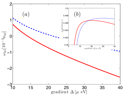
Figure 20: (color online). (a) Knight shift $\omega_{\mathrm{hf}}$ due to nonzero populations $p_{k}$ in the electronic quasisteady state for $t=20\mu\mathrm{eV}$ (solid) and $t=30\mu\mathrm{eV}$ (dashed). (b) In the high gradient regime, for $\Gamma\gg\Gamma_{\pm}$ the levels $\left|\lambda_{k}\right\rangle$ get depleted efficiently, such that $p_{k}<1\%\ll p$. Other numerical parameters: $\epsilon=30\mu\mathrm{eV}$ and $x_{\pm}=10^{-3}$.

In Section V we have analyzed the nuclear spin dynamics in the submanifold of the electronic quasisteady state $\rho_{\mathrm{ss}}^{\mathrm{el}}=\left(\left|T_{+}\right\rangle\left\langle T_{+}\right|+\left|T_{-}\right\rangle\left\langle T_{-}\right|\right)/2$. In this Appendix we consider (small) deviations from this ideal electronic quasisteady state due to populations of the levels $\left|\lambda_{k}\right\rangle\left(k=1,2,3\right)$, labeled as $p_{k}$. Since all coherences are damped out on electronic timescales, the generalized electronic quasisteady state under consideration is

$$\rho_{\mathrm{ss}}^{\mathrm{el}}=p\left(\left|T_{+}\right\rangle\left\langle T_{+}\right|+\left|T_{-}\right\rangle\left\langle T_{-}\right|\right)+\sum_{k}p_{k}\left|\lambda_{k}\right\rangle\left\langle\lambda_{k}\right|.$$ (191)

Using detailed balance, $p_{k}$ can be calculated via the equations $p_{k}\left(\kappa_{k}^{2}+x_{\pm}\right)=px_{\pm}$, where $x_{\pm}=\Gamma_{\pm}/\Gamma$ and $p=\left(1-\sum p_{k}\right)/2$ gives the population in $\left|T_{\pm}\right\rangle$, respectively. The electronic levels $\left|\lambda_{k}\right\rangle$ get depleted efficiently for $\Gamma_{k}\gg\Gamma_{\pm}$: In contrast to the low-gradient regime where $p_{2}\approx 1/3$, in the high-gradient regime, we obtain $p_{k}<1\%\ll p$ such that the electronic system settles to a quasisteady state very close to the ideal limit where $p=1/2$; compare Fig. 20. In describing the effective nuclear dynamics, nonzero populations $p_{k}$ lead to additional terms which are second order in $\varepsilon$, but strongly suppressed further as $p_{k}\ll 1$.

Knight shift.—For nonzero populations $p_{k}$, the Knight shift seen by the nuclear spins does not vanish, leading to the following (undesired) additional term for the effective nuclear spin dynamics

$$\dot{\sigma}=-i\omega_{\mathrm{hf}}\left[\delta A_{1}^{z}-\delta A_{2}^{z},\sigma\right],$$ (192)

where

$$\omega_{\mathrm{hf}}=\frac{a_{\mathrm{hf}}}{2}\sum_{k}p_{k}\left(\mu_{k}^{2}-\nu_{k}^{2}\right).$$ (193)

with $a_{\mathrm{hf}}\approx 10^{-4}\mu\mathrm{eV}$. As shown in Fig. 20, however, $\omega_{\mathrm{hf}}\approx 10^{-7}\mu\text{$\mathrm{eV}$}$ is further suppressed by approximately three orders of magnitude; in particular, $\omega_{\mathrm{hf}}$ is small compared to the dissipative gap of the nuclear dynamics $\mathrm{ADR}\approx 2\times 10^{-5}\mu\mathrm{eV}$ and can thus be neglected.

Hyperfine flip-flop dynamics.—Moreover, nonzero populations $p_{k}$ lead to additional Lindblad terms of the form $\dot{\sigma}=\dots+p_{k}\gamma_{k}^{+}\mathcal{D}[L_{k}^{\dagger}]\sigma$. They contain terms which are incommensurate with the ideal two-mode squeezedlike target state. Since $p_{k}\ll p$, however, they are strongly suppressed compared to the ones absorbed into $\mathcal{L}_{\mathrm{nid}}$ and thus do not lead to any significant changes in our analysis.

References

- (1) P. Zoller et al., Eur. Phys. J. D 36, 203 (2005).
- (2) M. A. Nielsen, I. L. Chuang, Quantum Computation and Quantum Information (Cambridge University Press, Cambridge, 2000).
- (3) R. Hanson, L. P. Kouwenhoven, J. R. Petta, S. Tarucha, and L. M. K. Vandersypen, Rev. Mod. Phys. 79, 1217 (2007).
- (4) D. D. Awschalom, N. Smarth, and D. Loss, Semiconductor Spintronics and Quantum Computation (Springer, New York, 2002).
- (5) E. A. Chekhovich, M. N. Makhonin, A. I. Tartakovskii, A. Yacoby, H. Bluhm, K. C. Nowack, and L. M. K. Vandersypen, Nat. Mat. 12, 494 (2013)
- (6) D. Loss and D. P. DiVincenzo, Phys. Rev. A 57, 120 (1998).
- (7) K. C. Nowack, F. H. L. Koppens, Y. V. Nazarov, and L. M. K. Vandersypen, Science 318, 1430 (2007).
- (8) K. C. Nowack, M. Shafiei, M. Laforest, G. E. D. K. Prawiroatmodjo, L. R. Schreiber, C. Reichl, W. Wegschneider, and L. M. K. Vandersypen, Science 333, 1269 (2011).
- (9) F. H. L. Koppens, J. A. Folk, J. M. Elzerman, R. Hanson, L. H. Willems van Beveren, I. T. Vink, H. P. Tranitz, W. Wegscheider, L. P. Kouwenhoven, and L. M. K. Vandersypen, Science 309, 1346 (2005).
- (10) F. H. L. Koppens, C. Buizert, K. J. Tielrooij, I. T. Vink, K. C. Nowack, T. Meunier, L. P. Kouwenhoven, and L. M. K. Vandersypen, Nature 442, 766 (2006).
- (11) J. R. Petta, A. C. Johnson, J. M. Taylor, E. A. Laird, A. Yacoby, M. D. Lukin, C. M. Marcus, M. P. Hanson, and A. C. Gossard, Science 309, 2180 (2005).
- (12) M. D. Shulman, O. E. Dial, S. P. Harvey, H. Bluhm, V. Umansky, and A. Yacoby, Science 336, 202 (2012).
- (13) J. Schliemann, A. Khaetskii, and Daniel Loss, J. Phys.: Condens. Matter 15, R1809 (2003).
- (14) W. A. Coish and D. Loss, Phys. Rev. B 70, 195340 (2004).
- (15) A. V. Khaetskii, D. Loss, and L. Glazman, Phys. Rev. Lett. 88, 186802 (2002).
- (16) I. A. Merkulov, Al. L. Efros, and M. Rosen, Phys. Rev. B 65, 205309 (2002).
- (17) S. I. Erlingsson, Yu. V. Nazarov, and V. I. Falko, Phys. Rev. B 64, 195306 (2001).
- (18) W. A. Coish, J. Fischer, and D. Loss, Phys. Rev. B 77, 125329 (2008).
- (19) L. Cywinski, W. M. Witzel, and S. Das Sarma, Phys. Rev. B 79, 245314 (2009).
- (20) A. C. Johnson, J. R. Petta, J. M. Taylor, A. Yacoby, M. D. Lukin, C. M. Marcus, M. P. Hanson, and A. C. Gossard, Nature 435, 925 (2005).
- (21) I. T. Vink, K. C. Nowack, F. H. L. Koppens, J. Danon, Y. V. Nazarov, and L. M. K. Vandersypen, Nat. Phys. 5, 764 (2009).
- (22) H. Bluhm, S. Foletti, I. Neder, M. Rudner, D. Mahalu, V. Umansky, and A. Yacoby, Nat. Phys. 7, 109 (2010).
- (23) S. Foletti, H. Bluhm, D. Mahalu, V. Umansky, and A. Yacoby, Nat. Phys. 5, 903 (2009).
- (24) K. Ono and S. Tarucha, Phys. Rev. Lett. 92, 256803 (2004).
- (25) K. Ono, D. G. Austing, Y. Tokura, and S. Tarucha, Science 297, 1313 (2002).
- (26) R. Takahashi, K. Kono, S. Tarucha, and K. Ono, Phys. Rev. Lett. 107, 026602 (2011).
- (27) J. M. Taylor, C. M. Marcus, and M. D. Lukin, Phys. Rev. Lett. 90, 206803 (2003).
- (28) Z. Kurucz, M. W. Sorensen, J. M. Taylor, M. D. Lukin, and M. Fleischhauer, Phys. Rev. Lett. 103, 010502 (2009).
- (29) J. M. Taylor, G. Giedke, H. Christ, B. Paredes, J. I. Cirac, P. Zoller, M. D. Lukin, A. Imamoglu, arXiv:cond-mat/0407640 (unpublished).
- (30) P. Cappellaro, L. Jiang, J. S. Hodges, and M. D. Lukin, Phys. Rev. Lett. 102, 210502 (2009).
- (31) W. M. Witzel and S. Das Sarma, Phys. Rev. B 76, 045218 (2007).
- (32) M. S. Rudner, L. M. K. Vandersypen, V. Vuletic, and L. S. Levitov, Phys. Rev. Lett. 107, 206806 (2011).
- (33) M. S. Rudner and L. S. Levitov, Phys. Rev. Lett. 99, 036602 (2007).
- (34) M. S. Rudner and L. S. Levitov, Phys. Rev. Lett. 99, 246602 (2007).
- (35) J. F. Poyatos, J. I. Cirac, and P. Zoller, Phys. Rev. Lett. 77, 4728 (1996).
- (36) F. Verstraete, M. M. Wolf, and J. I. Cirac, Nat. Phys. 5, 633 (2009).
- (37) S. Diehl, A. Micheli, A. Kantian, B. Kraus, H. P. Büchler, and P. Zoller, Nat. Phys. 4, 878 (2008).
- (38) R. Sanchez and G. Platero, Phys. Rev. B 87, 081305(R) (2013).
- (39) A. Tomadin, S. Diehl, M. D. Lukin, P. Rabl, and P. Zoller, Phys. Rev. A 86, 033821 (2012).
- (40) D. P. DiVincenzo, Fortschr. Phys. 48, 771 (2000).
- (41) C. A. Muschik, E. S. Polzik, and J. I. Cirac, Phys. Rev. A 83, 052312 (2011); H. Krauter, C. A. Muschik, K. Jensen, W. Wasilewski, J. M. Petersen, J. I. Cirac, and E. S. Polzik, Phys. Rev. Lett. 107, 080503 (2011).
- (42) J. T. Barreiro, M. Müller, P. Schindler, D. Nigg, T. Monz, M. Chwalla, M. Hennrich, C. F. Roos, P. Zoller, R. Blatt, Nature 470, 486 (2011).
- (43) Y. Lin, J. P. Gaebler, F. Reiter, T. R. Tan, R. Bowler, A. S. Sørensen, D. Leibfried, and D. J. Wineland, Nature 504, 415 (2013).
- (44) S. Shankar, M. Hatridge, Z. Leghtas, K. M. Sliwa, A. Narla, U. Vool, S. M. Girvin, L. Frunzio, M. Mirrahimi, and M. H. Devoret, Nature 504, 419 (2013).
- (45) M. J. A. Schuetz, E. M. Kessler, L. M. K. Vandersypen, J. I. Cirac, G. Giedke, Phys. Rev. Lett. 111, 246802 (2013).
- (46) M. J. A. Schuetz, E. M. Kessler, J. I. Cirac, and G. Giedke, Phys. Rev. B 86, 085322 (2012).
- (47) O. N. Jouravlev and Y. V. Nazarov, Phys. Rev. Lett. 96, 176804 (2006).
- (48) C. Lopez-Moniz, J. Inarrea, G. Platero, New J. Phys. 13, 053010 (2011).
- (49) S. E. Economou and E. Barnes, Phys. Rev. B 89, 165301 (2014).
- (50) M. S. Rudner, F. H. L. Koppens, J. A. Folk, L. M. K. Vandersypen, and L. S. Levitov, Phys. Rev. B 84, 075339 (2011).
- (51) J. Danon, I. T. Vink, F. H. L. Koppens, K. C. Nowack, L. M. K. Vandersypen, and Yu. V. Nazarov, Phys. Rev. Lett. 103, 046601 (2009).
- (52) A. M. Lunde, C. Lopez-Monis, I. A. Vasiliadou, L. L. Bonilla, and G. Platero, Phys. Rev. B 88, 035317 (2013).
- (53) J. R. Petta, J. M. Taylor, A. C. Johnson, A. Yacoby, M. D. Lukin, C. M. Marcus, M. P. Hanson, and A. C. Gossard, Phys. Rev. Lett. 100, 067601 (2008).
- (54) C. Barthel, J. Medford, H. Bluhm, A. Yacoby, C. M. Marcus, M. P. Hanson, and A. C. Gossard, Phys. Rev. B 85, 035306 (2012).
- (55) J. Baugh, Y. Kitamura, K. Ono, and S. Tarucha, Phys. Rev. Lett. 99, 096804 (2007).
- (56) T. Kobayashi, K. Hitachi, S. Sasaki, and K. Muraki, Phys. Rev. Lett. 107, 216802 (2011).
- (57) M. Gullans, J. J. Krich, J. M. Taylor, H. Bluhm, B. I. Halperin, C. M. Marcus, M. Stopa, A. Yacoby, and M. D. Lukin, Phys. Rev. Lett. 104, 226807 (2010).
- (58) T. Hayashi, T. Fujisawa, H. D. Cheong, Y. H. Jeong, and Y. Hirayama, Phys. Rev. Lett. 91, 226804 (2003).
- (59) C. Cohen-Tannoudji, J. Dupont-Roc, and G. Grynberg, Atom-Photon Interactions: Basic Processes and Applications (Wiley, New York, 1992).
- (60) G. Giavaras, N. Lambert, and F. Nori, Phys. Rev. B 87, 115416 (2013).
- (61) G. Petersen, E. A. Hoffmann, D. Schuh, W. Wegscheider, G. Giedke, and S. Ludwig, Phys. Rev. Lett. 110, 177602 (2013).
- (62) The analytic expressions for the amplitudes and are not instructive and therefore not explicitly given.
- (63) F. Qassemi, W. A. Coish, and F. K. Wilhelm, Phys. Rev. Lett. 102, 176806 (2009).
- (64) Note that, in the spirit of the approximation of independent rates of variation cohen-tannoudji92 , the relevant (in-)coherent couplings are shown in Fig. 3 in terms of the bare basis for . After a basis transformation to the dressed basis one obtains the dissipative terms given in Eq.(II.2).
- (65) If the nuclear spins in the second dot are highly polarized, the doubly occupied triplet levels get Zeeman split by the corresponding local Overhauser field. In principle, this could lead to a small asymmetry in the incoherent rates describing decay from to and vice versa. However, in the Appendix it is shown that in this regime a similar incoherent decay process within the Pauli-blocked triplet space can be made much more efficient by working in a regime of fast spin-exchange with the reservoirs in the leads.
- (66) Y. Yamamoto and A. Imamoglu, Mesoscopic Quantum Optics (Wiley, New York, 1999).
- (67) E. M. Kessler, Phys. Rev. A 86, 012126 (2012).
- (68) M. Pioro-Ladriere, T. Obata, Y. Tokura, Y.S. Shin, T. Kubo, K. Yoshida, T. Taniyama, and S. Tarucha, Nat. Phys. 4, 776 (2008).
- (69) Here, we have set for simplicity. However, similar results (not shown) have been obtained for finite values of .
- (70) H. Christ, J. I. Cirac, and G. Giedke, Phys. Rev. B 75, 155324 (2007).
- (71) H. Bluhm, S. Foletti, D. Mahalu, V. Umansky, and A. Yacoby, Phys. Rev. Lett. 105, 216803 (2010).
- (72) E. M. Kessler, G. Giedke, A. Imamoglu, S. F. Yelin, M. D. Lukin, and J. I. Cirac, Phys. Rev. A 86, 012116 (2012).
- (73) J. Laurat et al., J. Opt. B 7, 577 (2005).
- (74) H. Schwager, J. I. Cirac, and G. Giedke, New J. Phys. 12, 043026 (2010).
- (75) G. Giedke, M. M. Wolf, O. Kruger, R. F. Werner, and J. I. Cirac, Phys. Rev. Lett. 91, 107901 (2003).
- (76) M. M. Wolf, G. Giedke, O. Kruger, R. F. Werner, and J. I. Cirac, Phys. Rev. A 69, 052320 (2004).
- (77) G. Vidal and R. F. Werner, Phys. Rev. A 65, 032314 (2002).
- (78) D. Nagy, G. Szirmai, and P. Domokos, Phys. Rev. A 84, 043637 (2011).
- (79) F. Dimer, B. Estienne, A. S. Parkins, and H. J. Carmichael, Phys. Rev. A 75, 013804 (2007).
- (80) S. Diehl, A. Tomadin, A. Micheli, R. Fazio, and P. Zoller, Phys. Rev. Lett. 105, 015702 (2010).
- (81) M. Höning, M. Moos, and M. Fleischhauer, Phys. Rev. A 86, 013606 (2012).
- (82) H. Eleuch and I. Rotter, Eur. Phys. J. D 68, 74 (2014).
- (83) I. Lesanovsky, M. van Horssen, M. Gutua, and J. P. Garrahan, Phys. Rev. Lett. 110, 150401 (2013).
- (84) G. A. Alvarez, E. P. Danieli, P. R. Levstein, and H. M. Pastawski, J. Chem. Phys. 124, 194507 (2006).
- (85) E. P. Danieli, G. A. Alvarez, P. R. Levstein, and H. M. Pastawski, Solid State Commun. 141, 422 (2007).
- (86) H. Schwager, J. I. Cirac, and G. Giedke, Phys. Rev. B 81, 045309 (2010).
- (87) We have numerically checked that the entanglement generation persists for a small external gradient provided that the corresponding induced nuclear Zeeman splitting is small compared to the dissipative gap . Thus, to support the generation of steady-state entnaglement, we estimate that the magnetic gradient should be smaller than .
- (88) D. J. Reilly, J. M. Taylor, E. A. Laird, J. R. Petta, C. M. Marcus, M. P. Hanson, and A. C. Gossard, Phys. Rev. Lett. 101, 236803 (2008).
- (89) D. Paget, Phys. Rev. B 25, 4444 (1982).
- (90) M. S. Rudner and L. S. Levitov, Phys. Rev. Lett. 110, 086601 (2013).
- (91) O. E. Dial, M. D. Shulman, S. P. Harvey, H. Bluhm, V. Umansky, and A. Yacoby, Phys. Rev. Lett. 110, 146804 (2013).
- (92) K. Hammerer, A. S. Sørensen, and E. S. Polzik, Rev. Mod. Phy. 82, 1041 (2010).
- (93) A. Furusawa and N. Takei, Phys. Rep. 443, 97 (2007).
- (94) W. Wasilewski et al., Rev. Lett. 104, 133601 (2010).
- (95) J. Appel et al., Proc. Natl. Acad. Sci. U.S.A. 106, 10960 (2009).
- (96) M. H. Schleier-Smith, I. D. Leroux, and V. Vuletić, Rev. Lett. 104, 073604 (2010).
- (97) C. Gross et al., Nature 464, 1165 (2010); M. F. Riedel et al., Nature 464, 1170 (2010).
- (98) H. J. Kimble, Nature 453, 1023 (2008).
- (99) F. R. Braakman, P. Barthelemy, C. Reichl, W. Wegschneider, and L. M. K. Vandersypen, Nat. Nano. 8, 432 (2013).
- (100) M. Busl et al., Nat. Nano. 8, 261 (2013).
- (101) G. Feve, A. Mahe, J.-M. Berroir, T. Kontos, B. Placais, D. C. Glattli, A. Cavanna, B. Etienne, and Y. Jin, Science 316, 1169 (2007).
- (102) P. Roulleau, F. Portier, D. C. Glattli, P. Roche, A. Cavanna, G. Faini, U. Gennser, and D. Mailly, Phys. Rev. Lett. 100, 126802 (2008).
- (103) E. Bocquillon, V. Freulon, J.-M. Berroir, P. Degiovanni, B. Placais, A. Cavanna, Y. Jin, G. Feve, Science 339, 1054 (2013).
- (104) J. D. Fletcher et al., Phys. Rev. Lett. 111, 216807 (2013).
- (105) A. Mahe et al., Phys. Rev. B 82, 201309(R) (2010).
- (106) S. Hermelin, S. Takada, M. Yamamoto, S. Tarucha, A. D. Wieck, L. Saminadayar, C. Bäuerle, and T. Meunier, Nature 477, 435 (2011).
- (107) R. P. G. McNeil, M. Kataoka, C. J. B. Ford, C. H. W. Barnes, D. Anderson, G. A. C. Jones, I. Farrer, and D. A. Ritchie, Nature 477, 439 (2011).
- (108) M. Yamamoto, S. Takada, C. Bäuerle, K. Watanabe, A. D. Wieck, and S. Tarucha, Nat. Nano. 7, 247 (2012).
- (109) H. Sanada, Y. Kunihashi, H. Gotoh, K. Onomitsu, M. Kohda, J. Nitta, P. V. Santos, and T. Sogawa, Nat. Phys. 9, 280 (2013).
- (110) H. Christ, J. I. Cirac, and G. Giedke, Phys. Rev. B 78, 125314 (2008).
- (111) H. J. Carmichael, J. Phys. B 13, 3551 (1980).
- (112) S. Morrison and A. S. Parkins, Phys. Rev. A 77, 043810 (2008).
- (113) C.-H. Chung, K. Le Hur, M. Vojta, and P. Wolfle, Phys. Rev. Lett. 102, 216803 (2009).
- (114) L. Borda, G. Zarand, and D. Goldhaber-Gordon, arXiv:cond-mat/0602019.
- (115) A. J. Leggett, S. Chakravarty, A. T. Dorsey, M. P. A. Fisher, A. Garg, and W. Zwerger, Rev. Mod. Phys. 59, 1 (1987).
- (116) M. S. Rudner and L. S. Levitov, Phys. Rev. B 82, 155418 (2010).
- (117) D. Stepanenko, M. Rudner, B. I. Halperin, and D. Loss, Phys. Rev. B 85, 075416 (2012).
- (118) In deriving Eq.(110), we have ignored level shifts arising from the coupling to the environment; as usual, they can be absorbed into renormalized energy levels. Moreover, we have applied the so-called secular approximation which is mathematically correct in the weak coupling limit and ensures the positivity of the dynamics rivas12 .
- (119) A. Rivas and S. F. Huelga, Open Quantum System: An Introduction (Springer, Heidelberg, 2012).
- (120) Here, the tilde symbol explicitly refers to the dressed electronic basis . For notational convenience, it is dropped in the main text.
- (121) For simplicity, in the definition of we have included dissipative cotunneling-mediated transitions in the bare triplet subspace only . To make the comparison with the Liouvillian in the dressed basis , the corresponding mixing terms and in appear with a rate . In particular, in the low-gradient regime where this captures well the dissipative mixing between and which is the most adverse process to our scheme. We have also verified that simply replacing as it is stated in Eq.(II.2) does not change nor severely.
- (122) A. Uhlmann, Rep. Math. Phys. 9, 273 (1976).
- (123) L.P. Kouwenhoven, G. Schön, and L. Sohn, Proceedings of the NATO Advanced Study Institute on Mesoscopic Electron Transport, (Kluwer Academic Publishers, Dordrecht, 1997).
- (124) P. Recher, E. V. Sukhorukov, and D. Loss, Phys. Rev. Lett. 85, 1962 (2000).
- (125) H.-A. Engel and D. Loss, Phys. Rev. B 65, 195321 (2002).
- (126) L. R. Schreiber, F. R. Braakman, T. Meunier, V. Calado, J. Danon, J. M. Taylor, W. Wegschneider, and L. M. K. Vandersypen, Nat. Commun. 2, 556 (2011).
- (127) J. Danon and Yu. V. Nazarov, Phys. Rev. B 80, 041301(R) (2009).