A chiral effective field theory study of hadronic parity violation in few-nucleon systems

Abstract

We reconsider the derivation of the nucleon-nucleon parity-violating (PV) potential within a chiral effective field theory framework. We construct the potential up to next-to-next-to-leading order by including one-pion-exchange, two-pion-exchange, contact, and $1/M$ ($M$ being the nucleon mass) terms, and use dimensional regularization to renormalize the pion-loop corrections. A detailed analysis of the number of independent low-energy constants (LEC’s) entering the potential is carried out. We find that it depends on six LEC’s: the pion-nucleon PV coupling constant $h^{1}_{\pi}$ and five parameters multiplying contact interactions. We investigate PV effects induced by this potential on several few-nucleon observables, including the $\vec{p}\,$-$p$ longitudinal asymmetry, the neutron spin rotation in $\vec{n}$-$p$ and $\vec{n}$-$d$ scattering, and the longitudinal asymmetry in the ³He$(\vec{n},p)^{3}$H charge-exchange reaction. An estimate for the range of values of the various LEC’s is provided by using available experimental data.

I Introduction

A number of experiments aimed at studying hadronic parity violation in low-energy processes involving few nucleon systems are being completed, or are in an advanced stage of planning, at cold neutron facilities, such as the Los Alamos Neutron Science Center (LANSCE), the National Institute of Standards and Technology (NIST) Center for Neutron Research, and the Spallation Neutron Source (SNS) at Oak Ridge National Laboratory. The primary objective of this program is to determine the fundamental parameters of the parity-violating (PV) nucleon-nucleon ($NN$) potential (for a review of the current status of experiment and theory, see, for example, Refs. MP06 ; HH13 ; SS13 ).

Until a few years ago, the standard framework by which nuclear PV processes were analyzed theoretically was based on meson-exchange potentials, in particular the model proposed by Desplanques, Donoghue, and Holstein (DDH) DDH which included pion and vector-meson exchanges with seven unknown meson-nucleon PV coupling constants.

More recently, however, the emergence of chiral effective field theory ($\chi$EFT) Weinberg90 has provided renewed impetus to the development of nuclear forces in a field-theoretic framework ORVK96 ; Epelbaum09 ; ME11 . The $\chi$EFT approach is based on the observation that the chiral symmetry exhibited by quantum chromodynamics (QCD) severely restricts the form of the interactions of pions among themselves and with other particles W66 ; CCWZ69 . In particular, the pion couples to the nucleon by powers of its momentum $Q$, and the Lagrangian describing these interactions can be expanded in powers of $Q/\Lambda_{\chi}$, where $\Lambda_{\chi}\simeq 1$ GeV specifies the chiral symmetry breaking scale. As a consequence, classes of Lagrangians emerge, each characterized by a given power of $Q/\Lambda_{\chi}$ and each involving a certain number of unknown coefficients, so called low-energy constants (LEC’s), which are then determined by fits to experimental data (see, for example, the review papers Epelbaum09 ; Bernard95 and references therein).

Chiral effective field theory has been used to study two- and many-nucleon interactions Epelbaum09 ; ME11 and the interaction of electroweak probes with nuclei Park96 ; Park03 ; Pastore09 ; Koelling09 ; Pastore11 ; Koelling11 ; Piarulli13 . Its validity is restricted to processes occurring at low energies. In this sense, it has a more limited range of applicability than meson-exchange or more phenomenological models of these interactions, which in fact quantitatively and successfully account for a wide variety of nuclear properties and reactions up to energies, in some cases, well beyond the pion production threshold (for a review, see Ref. Carlson98 ). However, it is undeniable that $\chi$EFT has put nuclear physics on a more fundamental basis by providing, on the one hand, a direct connection between the QCD symmetries—in particular, chiral symmetry—and the strong and electroweak interactions in nuclei, and, on the other hand, a practical calculational scheme, which can, at least in principle, be improved systematically.

The $\chi$EFT approach has also been used to study PV $NN$ potentials, which are induced by hadronic weak interactions—these follow from weak interactions between quarks inside hadrons KS93 . It is well known that the weak interaction in the Standard Model contains both parity-conserving (PC) and PV components. The part of the weak interactions contributing to the PC $NN$ potential is obviously totally “hidden” by the strong and electromagnetic interactions, and is therefore not accessible experimentally. However, their PV part can be revealed in dedicated experiments. Since the fundamental weak Lagrangian of quarks is not invariant under chiral symmetry, one constructs the most general PV Lagrangian of nucleons and pions by requiring that the pattern of chiral symmetry breaking at the hadronic level be the same as at the quark level. Moreover, since the combination of charge conjugation ($C$) and parity ($P$) is known to be violated to a much lesser extent, it is customary to consider only $P$-violating but $CP$-conserving terms KS93 .

Following this scheme, Kaplan and Savage KS93 constructed an effective Lagrangian describing the interactions of pions and nucleons up to one derivative (i.e., at order $Q$). This Lagrangian includes at leading order (LO), or $Q^{0}$, a Yukawa-type pion-nucleon interaction with no derivatives. The coupling constant multiplying this term is denoted as $h^{1}_{\pi}$, the pion-nucleon weak coupling constant. It gives rise to a long-range, one-pion-exhange (OPE) contribution to the PV $NN$ potential. Many experiments have attempted to determine this long-range component and to obtain a determination of $h^{1}_{\pi}$, a task which has proven so far to be elusive (for a review see Ref. HH13 ). Very recently, an attempt has also been made to estimate the value of $h^{1}_{\pi}$ in a lattice QCD calculation Wasem2012 .

The Kaplan-Savage Lagrangian also includes five next-to-leading order (NLO) pion-nucleon interaction, or $Q^{1}$, terms with one derivative (and accompanying LEC’s), which, however, do not enter the PV $NN$ potential when considering processes at either tree level or one loop KS93 ; Zhu05 .

Since the pioneering study of Ref. KS93 , there have been several studies of the PV $NN$ potential in $\chi$EFT Zhu00 ; Zhu01 . The first derivation up to next-to-next-to-leading order (${\rm N2LO}$) was carried out by Zhu et al. Zhu05 . This potential includes the long-range OPE component, medium-range components originating from two-pion-exhange (TPE) processes, and short-range components deriving from ten four-nucleon contact terms involving one derivative of the nucleon field. In a subsequent analysis Girlanda08 , it was shown that there exist only five independent contact terms entering the potential at ${\rm N2LO}$, corresponding to the five PV S-P transition amplitudes at low energies Danilov65 . Zhu et al. Zhu05 also included three pion-nucleon PV interaction terms of order $Q^{2}$. This potential was recently used in a calculation of the longitudinal analyzing power in $\vec{p}$-$p$ scattering Vries13 .

In subsequent years, the ${\rm N2LO}$ contributions due to TPE and contact terms were independently studied in a series of papers Desp08 ; Liu07 ; Hyun07 ; Hyun08 by a different collaboration. In particular, this collaboration carried out a calculation of the photon asymmetry in the radiative capture ¹H$(\vec{n},\gamma)^{2}$H.

The objectives of the present work are twofold. The first is to reconsider the problem of how many independent PV Lagrangian terms are allowed at order $Q^{2}$, and to construct the complete PV $NN$ potential at ${\rm N2LO}$. A similar analysis for the parity- and time-reversal violating Lagrangian terms (with the aim to study the electric dipole moment of nucleons and light nuclei) has been recently reported in Ref. VMTK13 . The second objective is to use this potential to investigate PV effects in several processes involving few-nucleon systems, including the $\vec{p}\,$-$p$ longitudinal asymmetry, the neutron spin rotation in $\vec{n}$-$p$ and $\vec{n}$-$d$ scattering, and the longitudinal asymmetry in the ³He($\vec{n},p$)³H reaction, and to provide estimates for the values of the various LEC’s by fitting available experimental data.

To date, measurements are available for the following PV observables: the longitudinal analyzing power in $\vec{p}\,$-$p$ Balzer80 –Berdoz03 and $\vec{p}$-$\alpha$ Lang85 scattering, the photon asymmetry and photon circular polarization in, respectively, the ¹H($\vec{n},\gamma$)²H Cavaignac77 –Gericke09 and ¹H($n,\vec{\gamma}$)²H Knyazkov84 radiative captures, and the neutron spin rotation in $\vec{n}$-$\alpha$ scattering Snow09 ; Bass09 . The planned experiments include measurements of the neutron spin rotation in $\vec{n}$-$p$ Snow09 and $\vec{n}$-$d$ Markoff07 scattering, and of the longitudinal asymmetry in the charge-exchange reaction ³He($\vec{n},p$)³H at cold neutron energies Bowman07 . Recent studies of these observables in the framework of the DDH potential can be found in Refs. Schiavilla04 ; Schiavilla08 ; Viviani10 ; Gudkov10 ; Song11 ; Song12 .

We conclude this overview by noting that there exists a different approach to the derivation of PV (and PC) nuclear forces, based on an effective field theory in which pion degrees of freedom are integrated out (so called pionless EFT) and only contact interaction terms are considered. Such a theory, which is only valid at energies much less than the pion mass SS13 , has been used to study PV effects in nucleon-nucleon scattering PRR09 , PV asymmetries in the ¹H($\vec{n},\gamma$)²H capture SS09 , spin rotations in $\vec{n}$-$p$ and $\vec{n}$-$d$ scattering GSS11 , as well as other observables SS13 .

The present paper is organized as follows. In Sec. II we study the PV chiral Lagrangian up to order $Q^{2}$, while in Sec. III we derive the PV $NN$ potential at ${\rm N2LO}$. In Sec. IV, we report results obtained for the $\vec{p}\,$-$p$ longitudinal asymmetry, the neutron spin rotation in $\vec{n}$-$p$ and $\vec{n}$-$d$ scattering, and the longitudinal asymmetry in the ³He($\vec{n},p$)³H reaction, and provide estimates for the values of the various LEC’s. Finally, in Sec. V we present our conclusions and perspectives. A number of technical details are relegated in Appendices A-H.

II The PV Lagrangian

Weak interactions between quarks induce a PV $NN$ potential. This potential can be constructed starting from a pion-nucleon effective Lagrangian including all terms for which the pattern of chiral symmetry violation is the same as in the fundamental (quark-level) Lagrangian.

We begin with a brief summary of the building blocks used to construct the chiral Lagrangian (for reviews, see Refs. Epelbaum09 ; Bernard95 ; SS13 ). The pion field $\vec{\pi}$ enters the chiral Lagrangian via the unitary $SU(2)$ matrix

$$U=1+{i\over f_{\pi}}\vec{\tau}\cdot\vec{\pi}-{1\over 2f_{\pi}^{2}}\,\vec{\pi}^{\,2}-{i\alpha\over f_{\pi}^{3}}\,\vec{\pi}^{\,2}\,\vec{\tau}\cdot\vec{\pi}+{8\alpha-1\over 8f_{\pi}^{4}}\vec{\pi}^{\,4}+\ldots\ ,$$ (1)

where $f_{\pi}\simeq 92$ MeV is the bare pion decay constant and $\alpha$ is an arbitrary coefficient reflecting our freedom in the choice of the pion field. Observables must be independent of $\alpha$. Standard choices are $\alpha=0$ (non-linear sigma model) or $\alpha=1/6$, corresponding to the exponential parametrization $U=\exp(i\,\vec{\tau}\cdot\vec{\pi}/f_{\pi})$. In this and in the next section as well as in the Appendices, except for Appendix H, all the LEC’s entering the Lagrangian are to be considered as bare parameters. Renormalized LEC’s will be denoted by an overline above each symbol.

The other building blocks are $u=\sqrt{U}$ and

$$\nabla_{\mu}U = \partial_{\mu}U-ir_{\mu}U+iU\ell_{\mu}\ ,$$ (2)

$$u_{\mu} = i(u^{\dagger}\partial_{\mu}u-u\,\partial_{\mu}u^{\dagger})+u^{\dagger}r_{\mu}u-u\,\ell_{\mu}u^{\dagger}\ ,$$ (3)

$$\Gamma_{\mu} = {1\over 2}(u^{\dagger}\partial_{\mu}u+u\,\partial_{\mu}u^{\dagger})-\frac{i}{2}(u^{\dagger}r_{\mu}u+u\,\ell_{\mu}u^{\dagger})\ ,$$ (4)

$$\chi_{\pm} = u^{\dagger}\chi\,u^{\dagger}\pm u\,\chi^{\dagger}u\ ,$$ (5)

$$F_{\mu\nu}^{\pm} = u^{\dagger}F_{\mu\nu}^{R}u\pm u\,F_{\mu\nu}^{L}u^{\dagger}\ ,$$ (6)

$$X^{a}_{L} = u\,\tau_{a}u^{\dagger}\ ,\qquad\qquad X^{a}_{R}=u^{\dagger}\tau_{a}u\ ,$$ (7)

with

$$r_{\mu} = v_{\mu}+a_{\mu},\quad\ell_{\mu}=v_{\mu}-a_{\mu}\ ,\quad\chi=s+ip\ ,$$ (8)

$$F_{\mu\nu}^{R} = \partial_{\mu}r_{\nu}-\partial_{\nu}r_{\mu}-i[r_{\mu},r_{\nu}]\ ,$$ (9)

$$F_{\mu\nu}^{L} = \partial_{\mu}\ell_{\nu}-\partial_{\nu}\ell_{\mu}-i[\ell_{\mu},\ell_{\nu}]\ .$$ (10)

Here $v_{\mu}$, $a_{\mu}$, $p$, and $s$ are, respectively, $SU(2)$ matrices of vector, axial-vector, pseudoscalar, and scalar “external” fields, which are assumed to transform as

$$r_{\mu} \to R\,r_{\mu}R^{\dagger}+i\,R\,\partial_{\mu}R^{\dagger}\ ,$$ (11)

$$l_{\mu} \to L\,l_{\mu}L^{\dagger}+i\,L\,\partial_{\mu}L^{\dagger}\ ,$$ (12)

$$\chi \to R\,\chi\,L^{\dagger}\ ,$$ (13)

where $L$ ($R$) represents a local rotation in the isospin space of the left (right) components. The Lagrangian constructed in terms of these fields is invariant under local $SU(2)_{L}\times SU(2)_{R}$ chiral transformations.

In this paper we are interested in the $NN$ potential, and so ultimately we set $v_{\mu}=a_{\mu}=p=0$ and

$$s\to 2BM_{q}\ ,\qquad M_{q}=\left(\begin{array}[]{cc}m_{u}&0\\ 0&m_{d}\end{array}\right)\ ,$$ (14)

$m_{u}$, $m_{d}$ being the masses of “current” up and down quarks, respectively, and $B$ is a parameter related to the $\bar{q}q$ quark condensate, $B\,(m_{u}+m_{d})\sim m^{2}_{\pi}$, $m_{\pi}$ being the pion mass. Then, $\chi$ takes into account the explicit chiral symmetry breaking due to the non-vanishing current-quark masses. In the following, however, we construct all possible Lagrangian terms in the presence of external fields, since this will be useful when considering the coupling of nucleons and pions to electromagnetic and/or weak probes. In studying PV Lagrangian terms, it is customary to disregard isospin violation due to the $u$-$d$ quark mass difference, so we will assume $m_{u}=m_{d}$.

The transformation properties under the (non-linear) chiral symmetry $SU(2)_{L}\times SU(2)_{R}$ of the nucleon field $\psi$ and of the quantities defined in Eqs. (1)–(7) are the following (see, for example, Ref. Bernard95 )

$$U \rightarrow R\,U\,L^{\dagger}\qquad\qquad\nabla_{\mu}U\rightarrow R\,(\nabla_{\mu}U)\,L^{\dagger}\ ,$$

$$\psi \rightarrow h\,\psi\ ,\qquad\qquad u\rightarrow R\,u\,h^{\dagger}=h\,u\,L^{\dagger}\ ,$$

$$u_{\mu} \rightarrow h\,u_{\mu}h^{\dagger}\ ,\qquad\qquad\Gamma_{\mu}\rightarrow h\,\Gamma_{\mu}h^{\dagger}+h\,\partial_{\mu}h^{\dagger}\ ,$$ (15)

$$\chi_{\pm} \rightarrow h\chi_{\pm}h^{\dagger}\ ,\qquad\qquad F_{\mu\nu}^{\pm}\to h\,F_{\mu\nu}^{\pm}h^{\dagger}\ ,$$

$$X^{a}_{L} \rightarrow h\,u\,L^{\dagger}\tau_{a}L\,u^{\dagger}h^{\dagger}\ ,\qquad X^{a}_{R}\rightarrow h\,u^{\dagger}R^{\dagger}\tau_{a}R\,u\,h^{\dagger}\ ,$$

where $h$ is a $SU(2)$ matrix depending in a complicate way on $L$, $R$, and $\vec{\pi}(x)$, and expressing the non-linearity of the transformation. Note that the operator

$$D_{\mu}=\partial_{\mu}+\Gamma_{\mu}\ ,$$ (16)

when acting on the field $\psi$, transforms covariantly, namely

$$D_{\mu}\psi\rightarrow h\,D_{\mu}\psi\ .$$ (17)

The terms $\overline{\psi}X_{L}^{a}\psi$ and $\overline{\psi}X_{R}^{a}\psi$ transform like the operators $\overline{q}_{L}\tau_{a}q_{L}$ and $\overline{q}_{R}\tau_{a}q_{R}$, respectively, where $q$ represents the doublet of $u$ and $d$ quark fields, and $q_{L}$ and $q_{R}$ are the left and right components. Under $SU(2)_{L}\times SU(2)_{R}$ $q_{L}$ and $q_{R}$ transform as $q_{L}\rightarrow L\,q_{L}$ and $q_{R}\rightarrow R\,q_{R}$, and therefore

$$\overline{q}_{L}\tau_{a}q_{L}\rightarrow\overline{q}_{L}L^{\dagger}\tau_{a}\,L\,q_{L}\ ,\quad\overline{q}_{R}\tau_{a}q_{R}\rightarrow\overline{q}_{R}R^{\dagger}\tau_{a}\,R\,q_{R}\ .$$ (18)

Such terms enter the weak interaction Lagrangian at quark level. Therefore, quantities like $\overline{\psi}\,X_{L}^{a}\psi$ and $\overline{\psi}\,X_{R}^{a}\psi$ can be used to construct PV Lagrangian terms at hadronic level, which mimic the corresponding terms entering the weak interaction at quark level KS93 . For reasons mentioned earlier, the part of weak interaction contributing to the PC $NN$ potential is of no interest, and only $P$-violating but $CP$-conserving terms are considered below.

More precisely, at quark level the weak interaction includes terms which under chiral symmetry transform as isoscalar, isovector, and isotensor operators KS93 . At hadronic level, isoscalar terms can be constructed without involving the $X_{L,R}$ matrices, isovector terms are linear in $X_{L}$ or $X_{R}$, and isotensor terms involve combinations like ${\cal I}_{ab}(X^{a}_{L}X^{b}_{L}\pm X^{a}_{R}X^{b}_{R})$, where

$${\cal I}_{ab}=\left(\begin{array}[]{ccc}-1&0&0\\ 0&-1&0\\ 0&0&+2\\ \end{array}\right)\ .$$ (19)

Note that our definition of ${\cal I}_{ab}$ above is different from that commonly adopted in the literature. In the following, we also consider the quantities

$$X^{a}_{\pm}=X^{a}_{L}\pm X^{a}_{R}\ ,\qquad$$ (20)

which transform simply under $P$ and $C$, and use the notation $\langle\dots\rangle$ to denote the trace in flavor space, and define

$$\hat{A}=A-\frac{1}{2}\langle A\rangle\ .$$

The Lagrangian is ordered in classes of operators with increasing chiral dimension, according to the number of derivatives and/or quark mass insertions, e.g.,

$$u_{\mu}\sim Q\ ,\qquad F^{\pm}_{\mu\nu}\sim Q^{2}\ ,\qquad\chi_{\pm}\sim Q^{2}\ .$$

As per the covariant derivative $D_{\mu}$, it counts as $Q$, except when it acts on the nucleon field, in which case it is $Q^{0}$ due to the presence of the nucleon mass scale. The $\gamma^{5}$ matrix mixes the small and large components of the Dirac spinors, so that it should also be counted as $Q$. By considering all possible $P$-odd but $CP$-even interaction terms one can construct the most general Lagrangian. In doing so, use can be made of the equations of motion (EOM) for the nucleon and pion fields at lowest order, namely

$$iD_{\mu}\gamma^{\mu}\psi=\left(M+\frac{g_{A}}{2}\gamma_{5}\gamma^{\mu}u_{\mu}\right)\psi+{\cal O}(Q^{2})\ ,$$ (21)

$$[D_{\mu},u^{\mu}]=\frac{i}{2}\hat{\chi}_{-}+{\cal O}(Q^{4})\ ,$$ (22)

$M$ being the nucleon mass, and of a number of other identities,

$$[D_{\mu},D_{\nu}]=\frac{1}{4}[u_{\mu},u_{\nu}]-\frac{i}{2}F^{+}_{\mu\nu}\ ,$$ (23)

$$[D_{\mu},u_{\nu}]-[D_{\nu},u_{\mu}]=F^{-}_{\mu\nu}\ .$$ (24)

Note that covariant derivatives of $u_{\mu}$ only appear in the symmetrized form

$$h_{\mu\nu}=[D_{\mu},u_{\nu}]+[D_{\nu},u_{\mu}]\ ,$$ (25)

and that further simplifications follow from the Cayley-Hamilton relations, valid for any 2$\times$2 matrices $A$ and $B$,

$$AB+BA=A\langle B\rangle+B\langle A\rangle+\langle AB\rangle-\langle A\rangle\langle B\rangle\ ,$$ (26)

and from the traceless property of $u_{\mu}$ and $X^{a}_{L/R}$. As discussed before, we disregard isospin violation due to the $u$-$d$ quark mass difference, therefore, we assume $\chi=m_{\pi}^{2}\,I$ and set $\langle\chi_{-}\rangle=\langle F^{\mu\nu}_{-}\rangle=0$.

Care must be taken when constructing combinations of terms like $D_{\mu}X^{a}_{L/R}$, since they do not transform as given in Eq. (18), see discussion in Appendix A. There it is also shown that it is convenient to work instead with the following quantities

$$\left(X^{a}_{R}\right)_{\mu} = \left[D_{\mu}+iu^{\dagger}r_{\mu}u\,,\,X^{a}_{R}\right]\ ,$$ (27)

$$\left(X^{a}_{L}\right)_{\mu} = \left[D_{\mu}+iu\,\ell_{\mu}u^{\dagger}\,,\,X^{a}_{L}\right]\ .$$ (28)

These, in turn, reduce to

$$\left(X^{a}_{R}\right)_{\mu}={i\over 2}\left[u_{\mu}\,,\,X^{a}_{R}\right]\ ,\qquad\left(X^{a}_{L}\right)_{\mu}=-{i\over 2}\left[u_{\mu}\,,\,X^{a}_{L}\right]\ .$$ (29)

These identities are used in Appendix C in order to reduce the number of terms entering the PV Lagrangian.

We now first list the possible $\pi$-$N$ independent Lagrangian terms up to order $Q^{2}$. First, we need to recall the transformation properties of various quantities under hermitean conjugation, parity ($P$), and charge conjugation ($C$), which is done in Appendix B. The detailed discussion of the possible independent Lagrangian terms at order $Q^{2}$ is provided in Appendix C. We include in the definition of the interaction terms one power of the inverse nucleon mass for each covariant derivative $D_{\mu}$ acting on a nucleon field. All $Q^{2}$ terms have dimension (MeV)⁵.

II.1 The $\Delta I=0$ sector

In the $\Delta I=0$ sector, the Lagrangian starts at order $Q$ with one operator KS93 ,

$$O^{(0)}_{0V}=\bar{\psi}\gamma_{\mu}u^{\mu}\psi\ .$$ (30)

At order $Q^{2}$, as shown in Appendix C.1, we find the following two operators

$$O^{(0)}_{1}={1\over M}\bar{\psi}\gamma^{\mu}\gamma^{5}D^{\nu}\psi\langle u_{\mu}u_{\nu}\rangle+{\mathrm{h.c.}}\ ,$$ (31)

$$O^{(0)}_{2}=\bar{\psi}F^{-}_{\mu\nu}\sigma^{\mu\nu}\psi\ ,$$ (32)

where ${\mathrm{h.c.}}$ stands for the hermitean conjugate.

II.2 The $\Delta I=1$ sector

In the $\Delta I=1$ sector the Lagrangian, linear in the $X^{a}_{R/L}$ operators, starts at order $Q^{0}$ with

$$O^{(1)}_{\pi}=\bar{\psi}X^{3}_{-}\psi\ .$$ (33)

At order $Q$ there are two additional operators KS93 ,

$$O^{(1)}_{1V} = \bar{\psi}\gamma^{\mu}\psi\langle u_{\mu}X^{3}_{+}\rangle\ ,$$ (34)

$$O^{(1)}_{1A} = \bar{\psi}\gamma^{\mu}\gamma_{5}\psi\langle u_{\mu}X^{3}_{-}\rangle\ .$$ (35)

At order $Q^{2}$, there are many possibilities; however, as discussed in Appendix C.2, we consider the following combinations:

$$O^{(1)}_{1} = \bar{\psi}\psi\langle\hat{\chi}_{+}X^{3}_{-}\rangle\ ,$$ (36)

$$O^{(1)}_{2} = \bar{\psi}X^{3}_{-}\psi\langle\chi_{+}\rangle\ ,$$ (37)

$$O^{(1)}_{3} = \bar{\psi}[\hat{\chi}_{-},X^{3}_{+}]\psi\ ,$$ (38)

$$O^{(1)}_{4} = \bar{\psi}[X^{3}_{+},[u_{\mu},u_{\nu}]]\sigma_{\alpha\beta}\epsilon^{\mu\nu\alpha\beta}\psi\ ,$$ (39)

$$O^{(1)}_{5} = \bar{\psi}X^{3}_{-}\psi\langle u_{\mu}u^{\mu}\rangle\ ,$$ (40)

$$O^{(1)}_{6} = \bar{\psi}\sigma^{\mu\nu}\psi\langle X^{3}_{-}i[u_{\mu},u_{\nu}]\rangle\ ,$$ (41)

$$O^{(1)}_{7} = \bar{\psi}u_{\mu}X^{3}_{-}u^{\mu}\psi\ ,$$ (42)

$$O^{(1)}_{8} = {1\over M}\bar{\psi}X^{3}_{+}\gamma^{\mu}\gamma^{5}D^{\nu}\psi\langle u_{\mu}u_{\nu}\rangle+{\mathrm{h.c.}}\ ,$$ (43)

$$O^{(1)}_{9} = {1\over M}\bar{\psi}(u_{\mu}X^{3}_{+}u_{\nu}\!+\!u_{\nu}X^{3}_{+}u_{\mu})\gamma^{\mu}\gamma^{5}D^{\nu}\psi\!+\!{\mathrm{h.c.}}\ ,$$ (44)

$$O^{(1)}_{10} = {1\over M}\bar{\psi}X^{3}_{-}\gamma^{\mu}D^{\nu}\psi\langle u_{\mu}u_{\nu}\rangle+{\mathrm{h.c.}}\ ,$$ (45)

$$O^{(1)}_{11} = {1\over M}\bar{\psi}(u_{\mu}X^{3}_{-}u_{\nu}+u_{\nu}X^{3}_{-}u_{\mu})\gamma^{\mu}D^{\nu}\psi+{\mathrm{h.c.}}\ ,$$ (46)

$$O^{(1)}_{12} = {1\over M}\bar{\psi}[h_{\mu\nu},X^{3}_{+}]\gamma^{\mu}D^{\nu}\psi+{\mathrm{h.c.}}\ ,$$ (47)

$$O^{(1)}_{13} = {1\over M}\bar{\psi}[h_{\mu\nu},X^{3}_{-}]\gamma^{\mu}\gamma^{5}D^{\nu}\psi+{\mathrm{h.c.}}\ ,$$ (48)

$$O^{(1)}_{14} = \bar{\psi}i[\hat{F}_{+}^{\mu\nu},X^{3}_{+}]\sigma^{\alpha\beta}\epsilon_{\mu\nu\alpha\beta}\psi\ ,$$ (49)

$$O^{(1)}_{15} = \bar{\psi}\sigma_{\mu\nu}\psi\langle\hat{F}_{+}^{\mu\nu}X^{3}_{-}\rangle\ ,$$ (50)

$$O^{(1)}_{16} = \bar{\psi}X^{3}_{-}\sigma_{\mu\nu}\psi\langle F_{+}^{\mu\nu}\rangle\ .$$ (51)

$$O^{(1)}_{17} = \bar{\psi}\sigma_{\mu\nu}\psi\langle F_{-}^{\mu\nu}X^{3}_{+}\rangle\ ,$$ (52)

$$O^{(1)}_{18} = \bar{\psi}i[F_{-}^{\mu\nu},X^{3}_{-}]\sigma^{\alpha\beta}\epsilon_{\mu\nu\alpha\beta}\psi\ .$$ (53)

For operators $O^{(1)}_{9}$, $O^{(1)}_{11}$, and $O^{(1)}_{12}$, we have not explicitly written down all possible isospin combinations, but have reported only the simplest ones. When using these operators to construct interaction vertices by expanding in powers of the pion field, all allowed possibilities should be considered (see Appendix C.2).

II.3 The $\Delta I=2$ sector

The $\Delta I=2$ operators have to be constructed as combinations of ${\cal I}^{ab}(X^{a}_{R}\,O\,X^{b}_{R}\pm X^{a}_{L}\,O\,X^{b}_{L})$, with $O$ an operator transforming as $O\to h\,Oh^{\dagger}$. Since ${\cal I}^{ab}$ is diagonal and traceless, we have ${\cal I}^{ab}X^{a}_{R}\,X^{b}_{R}={\cal I}^{ab}X^{a}_{L}\,X^{b}_{L}=0$, therefore $O$ cannot be the identity. Moreover, combinations like ${\cal I}^{ab}(X^{a}_{R}\,O\,X^{b}_{L}\pm X^{a}_{R}\,O\,X^{b}_{L})$ are excluded since they do not appear in the Standard Model weak Lagrangian KS93 . At order $Q$ there are two possible operators KS93 ,

$$O^{(2)}_{2V} = {\cal I}^{ab}\bar{\psi}(X^{a}_{R}u_{\mu}X^{b}_{R}+X^{a}_{L}u_{\mu}X^{b}_{L})\gamma^{\mu}\psi\ ,$$ (54)

$$O^{(2)}_{2A} = {\cal I}^{ab}\bar{\psi}(X^{a}_{R}u_{\mu}X^{b}_{R}-X^{a}_{L}u_{\mu}X^{b}_{L})\gamma^{\mu}\gamma^{5}\psi\ .$$ (55)

At order $Q^{2}$, as discussed in Appendix C.3, we find the following eight possible operators:

$$O^{(2)}_{1} = {\cal I}^{ab}\bar{\psi}X^{a}_{R}\hat{\chi}_{+}X^{b}_{R}\psi-(R\leftrightarrow L)\ ,$$ (56)

$$O^{(2)}_{2} = {\cal I}^{ab}\bar{\psi}\Bigl{[}u_{\mu}X^{a}_{R}u_{\nu}X^{b}_{R}+X^{a}_{R}u_{\nu}X^{b}_{R}u_{\mu}$$ (57)

$$+ u_{\nu}X^{a}_{R}u_{\mu}X^{b}_{R}\!+\!X^{a}_{R}u_{\mu}X^{b}_{R}u_{\nu}\!-\!(R\leftrightarrow L)\Bigr{]}g^{\mu\nu}\psi\ ,$$

$$O^{(2)}_{3} = i\,{\cal I}^{ab}\bar{\psi}\Bigl{[}u_{\mu}X^{a}_{R}u_{\nu}X^{b}_{R}-X^{a}_{R}u_{\nu}X^{b}_{R}u_{\mu}$$ (58)

$$\qquad\quad-u_{\nu}X^{a}_{R}u_{\mu}X^{b}_{R}+X^{a}_{R}u_{\mu}X^{b}_{R}u_{\nu}$$

$$\qquad\quad-(R\leftrightarrow L)\Bigr{]}\sigma^{\mu\nu}\psi\ ,$$

$$O^{(2)}_{4} = i\,{\cal I}^{ab}\bar{\psi}\Bigl{[}X^{a}_{R}[u_{\mu}\,,\,u_{\nu}]X^{b}_{R}-(R\leftrightarrow L)\Bigr{]}\sigma^{\mu\nu}\psi\ ,$$ (59)

$$O^{(2)}_{5} = \bar{\psi}\{D_{\alpha}\,,\,\overline{Y}^{(1)}_{+,\mu\nu}\}g^{\alpha\mu}\gamma^{\nu}\gamma^{5}\psi\ ,$$ (60)

$$O^{(2)}_{6} = \bar{\psi}\{D_{\alpha}\,,\,\overline{Y}^{(1)}_{-,\mu\nu}\}g^{\alpha\mu}\gamma^{\nu}\psi\ ,$$ (61)

$$O^{(2)}_{7} = {\cal I}^{ab}\bar{\psi}\Bigl{[}X^{a}_{R}F^{+}_{\mu\nu}X^{b}_{R}-(R\leftrightarrow L)\Bigr{]}\sigma^{\mu\nu}\psi\ ,$$ (62)

$$O^{(2)}_{8} = {\cal I}^{ab}\bar{\psi}\Bigl{[}X^{a}_{R}F^{-}_{\mu\nu}X^{b}_{R}+(R\leftrightarrow L)\Bigr{]}\sigma^{\mu\nu}\psi\ ,$$ (63)

where the quantities $\overline{Y}^{(1)}_{\pm,\,\mu\nu}$ are defined in Eq. (160). In this case too for some of the operators we have not explicitly written down all possible isospin combinations, but reported only the simplest ones (see Appendix C.3).

II.4 Terms with only pionic degrees of freedom

Possible $\Delta I=0$ PV terms constructed with only pionic degrees of freedom, namely terms involving $\nabla_{\mu}U$ together with $\epsilon^{\mu\nu\alpha\beta}$ factors, turn out to vanish. Considering also terms involving the quantities $F_{\mu\nu}^{\pm}$, we find at order $Q^{4}$ the following $P$- and $C$-odd terms:

$$\langle\nabla^{\mu}U^{\dagger}\nabla^{\nu}UF_{\mu\nu}^{R}-\nabla^{\mu}U\nabla^{\nu}U^{\dagger}F_{\mu\nu}^{L}\rangle\ ,$$ (64)

$$\langle UF_{\mu\nu}^{R}U^{\dagger}F^{R\mu\nu}-UF_{\mu\nu}^{L}U^{\dagger}F^{L\mu\nu}\rangle\ .$$ (65)

Possible PV terms involving $\chi$, such as $\langle U\chi^{\dagger}-\chi U^{\dagger}\rangle$, are even under $C$.

Terms with $\Delta I=1$ and $\Delta I=2$ can be constructed using the quantities $X_{L,R}^{a}$. We find at order $Q^{2}$ the following two $P$- and $C$-odd operators

$$O^{(1)}_{\pi\pi\pi}=\langle u_{\mu}X^{3}_{-}u^{\mu}\rangle\ ,\,\,O^{(2)}_{\pi\pi\pi}={\cal I}^{ab}\langle X^{a}_{R}u_{\mu}X^{b}_{R}u^{\mu}-(R\rightarrow L)\rangle\ .$$ (66)

At lowest order, these terms give two three-pion vertices. However, their contribution to the PV potential is at least of order $Q^{2}$. Therefore, in the rest of the present work, we disregard the contributions of these PV terms.

II.5 Summary

The $\chi$EFT PV Lagrangian up to order $Q^{2}$ includes all terms determined above, each multiplied by a different low-energy constant (LEC), that is

$$\mathcal{L}^{PV} = \frac{h^{1}_{\pi}}{2\sqrt{2}}f_{\pi}\overline{\psi}X^{3}_{-}\psi+{h^{0}_{V}\over 2}\overline{\psi}\gamma^{\mu}u_{\mu}\psi$$ (67)

$$+ \frac{h_{V}^{1}}{4}\overline{\psi}\gamma^{\mu}\psi\langle u_{\mu}X^{3}_{+}\rangle+\frac{h_{A}^{1}}{4}\overline{\psi}\gamma^{\mu}\gamma^{5}\psi\langle u_{\mu}X^{3}_{-}\rangle$$

$$- {1\over 3}\,{\cal I}_{ab}\biggl{[}\frac{h_{V}^{2}}{2}\overline{\psi}\left(X^{a}_{R}u_{\mu}X^{b}_{R}+X^{a}_{L}u_{\mu}X^{b}_{L}\right)\gamma^{\mu}\psi$$

$$\quad+\frac{h_{A}^{2}}{4}\overline{\psi}\left(X^{a}_{R}u_{\mu}X^{b}_{R}-X^{a}_{L}u_{\mu}X^{b}_{L}\right)\gamma^{\mu}\gamma^{5}\psi\biggr{]}$$

$$-\sum_{p=1,2}{h^{0}_{p}\over f_{\pi}}O^{(0)}_{p}-\sum_{p=1,18}{h^{1}_{p}\over f_{\pi}}O^{(1)}_{p}$$

$$-\sum_{p=1,8}{h^{2}_{p}\over f_{\pi}}O^{(2)}_{p}+\mathcal{L}^{PV}_{CT}\ ,$$

where for the LEC’s multiplying the terms up to order $Q$ we have adopted the notation of Ref. Zhu00 (the different signs and numerical factors account for our different definition of $u_{\mu}$, $X^{3}_{-}$ and ${\cal I}_{ab}$). We have included in the last two lines the 28 terms of order $Q^{2}$ discussed in Subsec. II.1, II.2, and II.3. The Lagrangian contains also four-nucleon contact terms (included in $\mathcal{L}^{PV}_{CT}$), representing interactions originating from excitation of $\Delta$-resonances and exchange of heavy mesons. At lowest order, $\mathcal{L}^{PV}_{CT}$ contains five independent four-nucleon contact terms with a single gradient, as discussed in Ref. Girlanda08 .

The Lagrangian describing pion-nucleon interactions up to one derivative was already given by Kaplan and Savage KS93 . The LEC $h^{1}_{\pi}$ is the long-sought pion-nucleon PV coupling constant. By construction, it and all other LEC’s are adimensional (the factor $1/f_{\pi}$ has been introduced for convenience). In principle, the LEC’s can be determined by fitting experimental data or from lattice calculations (or from a combination of both methods). The order of magnitude of the various constants is

$$h\sim G_{F}f_{\pi}^{2}\approx 10^{-7}\ ,$$ (68)

which is also the order of magnitude of PV effects in few-nucleon systems.

In the following, we also need the PC Lagrangian up to order $Q^{2}$:

$${\cal L}^{PC} = {\cal L}_{\pi\pi}^{(2)}+{\cal L}_{\pi\pi}^{(4)}+\ldots$$ (69)

$$+ {\cal L}_{N\pi}^{(1)}+{\cal L}_{N\pi}^{(2)}+{\cal L}_{N\pi}^{(3)}+\ldots+{\cal L}^{PC}_{CT}\ ,$$

$${\cal L}_{\pi\pi}^{(2)} = {f_{\pi}^{2}\over 4}\langle\nabla_{\mu}U^{\dagger}\nabla^{\mu}U+\chi^{\dagger}U+\chi U^{\dagger}\rangle\ ,$$ (70)

$${\cal L}_{\pi\pi}^{(4)} = {1\over 16}\ell_{3}\Bigl{[}\langle\chi^{\dagger}U+\chi U^{\dagger}\rangle\Bigr{]}^{2}$$ (71)

$$+{1\over 8}\ell_{4}\Bigl{[}\langle\nabla_{\mu}U^{\dagger}\nabla^{\mu}U\rangle\langle\chi^{\dagger}U+\chi U^{\dagger}\rangle$$

$$\qquad-{1\over 2}(\langle\chi^{\dagger}U+\chi U^{\dagger}\rangle)^{2}\Bigr{]}+\ldots\ ,$$

$${\cal L}_{N\pi}^{(1)} = \overline{\psi}\Bigl{(}i\gamma^{\mu}D_{\mu}-M+{g_{A}\over 2}\gamma^{\mu}\gamma^{5}u_{\mu}\Bigr{)}\psi\ ,$$ (72)

$${\cal L}_{N\pi}^{(2)} = c_{1}\overline{\psi}\langle\chi_{+}\rangle\psi+\ldots\ ,$$ (73)

$${\cal L}_{N\pi}^{(3)} = d_{16}\overline{\psi}{1\over 2}\gamma^{\mu}\gamma^{5}u_{\mu}\langle\chi_{+}\rangle\psi$$ (74)

$$+ d_{18}\overline{\psi}{i\over 2}\gamma^{\mu}\gamma^{5}[D_{\mu},\chi_{-}]\psi+\cdots\ ,$$

where we have omitted terms not relevant in the present work (the complete ${\cal L}_{\pi\pi}^{(4)}$ can be found in Ref. GL84 and the complete ${\cal L}_{N\pi}^{(2)}$ and ${\cal L}_{N\pi}^{(3)}$ in Ref. Fettes00 ). Four-nucleon contact terms (see, for example, Refs.Epelbaum09 ; ME11 ) are lumped into ${\cal L}^{PC}_{CT}$. The parameters $\ell_{3}$, $\ell_{4}$, $c_{1}$, $d_{16}$, and $d_{18}$ are LEC’s entering the PC Lagrangian. To this Lagrangian, we add two mass counterterms

$${\cal L}_{MCT}=-{1\over 2}\delta m_{\pi}^{2}\,\vec{\pi}^{\,2}-\delta M\,\overline{\psi}\psi\ ,$$ (75)

which renormalize the pion ($m_{\pi}$) and nucleon ($M$) masses in ${\cal L}^{PC}$. The determination of $\delta M$ and $\delta m^{2}$ is discussed in Appendix G.

III The PV potential up to order $Q$

In this section, we discuss the derivation of the PV $NN$ potential at ${\rm N2LO}$. First, we provide, order by order in the power counting, formal expressions for it in terms of time-ordered perturbation theory (TOPT) amplitudes, and next discuss the various diagrams associated with these amplitudes (additional details are given in Appendix G).

III.1 From amplitudes to potentials

We begin by considering the conventional perturbative expansion for the $NN$ scattering amplitude

$$\langle N^{\prime}N^{\prime}\mid T\mid NN\rangle$$

$$=\langle N^{\prime}N^{\prime}\mid H_{I}\sum_{n=1}^{\infty}\left(\frac{1}{E_{i}-H_{0}+i\,\eta}H_{I}\right)^{n-1}\mid NN\rangle\ ,$$ (76)

where $\mid NN\rangle$ and $\mid N^{\prime}N^{\prime}\rangle$ represent the initial and final two-nucleon states of energy $E_{i}$, $H_{0}$ is the Hamiltonian describing free pions and nucleons, and $H_{I}$ is the Hamiltonian describing interactions among these particles. The evaluation of this amplitude is carried out in practice by inserting complete sets of $H_{0}$ eigenstates between successive $H_{I}$ terms. Power counting is then used to organize the expansion in powers of $Q/\Lambda_{\chi}\ll 1$, where $\Lambda_{\chi}\simeq 1$ GeV is the typical hadronic mass scale,

$$\langle N^{\prime}N^{\prime}|T|NN\rangle=\sum_{n}T^{(n)},$$ (77)

where $T^{(n)}\sim Q^{n}$. We note that in Eq. (76) the interaction Hamiltonian $H_{I}$ is in the Schrödinger picture and that, at the order of interest here, it follows simply from $H_{I}=-\int{\rm d}{\bm{x}}\;{\cal L}_{I}(t=0,{\bm{x}})$. Vertices from $H_{I}$ are listed in Appendix F.

We obtain the $NN$ potential $V$ by requiring that iterations of it in the Lippmann-Schwinger (LS) equation

$$V+V\,G_{0}\,V+V\,G_{0}\,V\,G_{0}\,V+\dots\ ,$$ (78)

lead to the $T$-matrix in Eq. (77), order by order in the power counting. In practice, this requirement can only be satisfied up to a given order $n^{*}$, and the resulting potential, when inserted into the LS equation, will generate contributions of order $n>n^{*}$, which do not match $T^{(n)}$. In Eq. (78), $G_{0}$ denotes the free two-nucleon propagator, $G_{0}=1/(E_{i}-H_{0}+i\,\eta)$, and we assume that

$$\langle N^{\prime}N^{\prime}|V|NN\rangle=\sum_{n}V^{(n)}\ ,$$ (79)

where the yet to be determined $V^{(n)}$ is of order $Q^{n}$. We also note that, generally, a term like $\left[V^{(m)}\,G_{0}\,V^{(n)}\right]$ is of order $Q^{m+n+1}$, since $G_{0}$ is of order $Q^{-2}$ and the implicit loop integration brings in a factor $Q^{3}$ (for a more detailed discussion see Ref. Pastore11 ).

We now consider the case of interest here, in which the two nucleons interact via a PC potential plus a very small PV component. The $\chi$EFT Hamiltonian implies the following expansion in powers of $Q$ for $T=T_{PC}+T_{PV}$:

$$T_{PC} = T^{(0)}_{PC}+T^{(1)}_{PC}+T^{(2)}_{PC}+\ldots,$$ (80)

$$T_{PV} = T^{(-1)}_{PV}+T^{(0)}_{PV}+T^{(1)}_{PV}+\ldots.$$ (81)

We assume that $V=V_{PC}+V_{PV}$ have a similar expansion,

$$V_{PC} = V_{PC}^{(0)}+V_{PC}^{(1)}+V_{PC}^{(2)}+\dots$$ (82)

$$V_{PV} = V_{PV}^{(-1)}+V_{PV}^{(0)}+V_{PV}^{(1)}+\dots,$$ (83)

and to linear terms in $V_{PV}$ we find

$$T = V+VG_{0}V+VG_{0}VG_{0}V+\cdots$$ (84)

$$= V_{PC}+V_{PV}$$

$$+ V_{PC}G_{0}V_{PC}\!+\!V_{PV}G_{0}V_{PC}\!+\!V_{PC}G_{0}V_{PV}$$

$$+ V_{PC}G_{0}V_{PC}G_{0}V_{PC}\!+\!V_{PV}G_{0}V_{PC}G_{0}V_{PC}$$

$$+ V_{PC}G_{0}V_{PV}G_{0}V_{PC}\!+\!V_{PC}G_{0}V_{PC}G_{0}V_{PV}\!+\!\cdots\ .$$

By matching up to the order $Q^{2}$ for $V_{PC}$ and $Q^{1}$ for $V_{PV}$, we obtain for the PC potential

$$V_{PC}^{(0)} = T_{PC}^{(0)}\ ,$$ (85)

$$V_{PC}^{(1)} = T_{PC}^{(1)}-\left[V_{PC}^{(0)}G_{0}V_{PC}^{(0)}\right]\ ,$$ (86)

$$V_{PC}^{(2)} = T_{PC}^{(2)}-\left[V_{PC}^{(0)}G_{0}V_{PC}^{(1)}\right]-\left[V_{PC}^{(1)}G_{0}V_{PC}^{(0)}\right]$$ (87)

$$- \left[V_{PC}^{(0)}G_{0}V_{PC}^{(0)}G_{0}V_{PC}^{(0)}\right]\ ,$$

and for the PV one

$$V_{PV}^{(-1)} = T_{PV}^{(-1)}\ ,$$ (88)

$$V_{PV}^{(0)} = T_{PV}^{(0)}-\left[V_{PV}^{(-1)}G_{0}V_{PC}^{(0)}\right]-\left[V_{PC}^{(0)}G_{0}V_{PV}^{(-1)}\right]\ ,$$ (89)

$$V_{PV}^{(1)} = T_{PV}^{(1)}-\left[V_{PV}^{(0)}G_{0}V_{PC}^{(0)}\right]-\left[V_{PC}^{(0)}G_{0}V_{PV}^{(0)}\right]$$ (90)

$$- \left[V_{PV}^{(-1)}G_{0}V_{PC}^{(1)}\right]-\left[V_{PC}^{(1)}G_{0}V_{PV}^{(-1)}\right]$$

$$- \left[V_{PV}^{(-1)}G_{0}V_{PC}^{(0)}G_{0}V_{PC}^{(0)}\right]-\left[V_{PC}^{(0)}G_{0}V_{PV}^{(-1)}G_{0}V_{PC}^{(0)}\right]$$

$$- \left[V_{PC}^{(0)}G_{0}V_{PC}^{(0)}G_{0}V_{PV}^{(-1)}\right]\ .$$

The expressions above relate $V^{(n)}_{PC}$ and $V^{(n)}_{PV}$ to the $T^{(n)}_{PC}$ and $T^{(n)}_{PV}$ amplitudes.

III.2 The PV potential

It is convenient to define the following momenta

$${\bm{K}}_{j}=({\bm{p}}_{j}^{\prime}+{\bm{p}}_{j})/2\ ,\quad{\bm{k}}_{j}={\bm{p}}_{j}^{\prime}-{\bm{p}}_{j}\ ,$$ (91)

where ${\bm{p}}_{j}$ and ${\bm{p}}^{\prime}_{j}$ are the initial and final momenta of nucleon $j$. Since ${\bm{k}}_{1}=-{\bm{k}}_{2}={\bm{k}}$ from overall momentum conservation ${\bm{p}}_{1}+{\bm{p}}_{2}={\bm{p}}_{1}^{\prime}+{\bm{p}}_{2}^{\prime}$, the momentum-space matrix element of the potential $V$ is a function of the momentum variables ${\bm{k}}$, ${\bm{K}}_{1}$, and ${\bm{K}}_{2}$, namely

$$\langle\alpha_{1}^{\prime}\alpha_{2}^{\prime}|V_{PV}|\alpha_{1}\alpha_{2}\rangle={1\over\Omega}V_{PV}({\bm{k}},{\bm{K}}_{1},{\bm{K}}_{2})\delta_{{\bm{p}}_{1}+{\bm{p}}_{2},{\bm{p}}_{1}^{\prime}+{\bm{p}}_{2}^{\prime}}\ ,$$ (92)

where $\alpha_{j}\equiv\{{\bm{p}}_{j},s_{j},t_{j}\}$ denotes the momentum, spin projection, and isospin projection of nucleon $j$, and the various momenta are discretized by assuming periodic boundary conditions in a box of volume $\Omega$. Moreover, we can write

$$V_{PV}({\bm{k}},{\bm{K}}_{1},{\bm{K}}_{2})=V_{PV}^{(CM)}({\bm{k}},{\bm{K}})+V^{({\bm{P}})}_{PV}({\bm{k}},{\bm{K}})\ ,$$ (93)

where ${\bm{K}}=({\bm{K}}_{1}-{\bm{K}}_{2})/2$, ${\bm{P}}={\bm{p}}_{1}+{\bm{p}}_{2}={\bm{K}}_{1}+{\bm{K}}_{2}$, and the term $V^{({\bm{P}})}_{PV}({\bm{k}},{\bm{K}})$ represents boost corrections to $V^{(CM)}_{PV}({\bm{k}},{\bm{K}})$ Girlanda10 , the potential in the center-of-mass (CM) frame. Below we ignore these boost corrections and provide expressions for $V^{(CM)}_{PV}({\bm{k}},{\bm{K}})$ only.

.

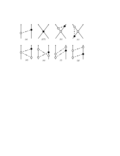
Figure 1: Time-ordered diagrams contributing to the PV potential (only a single time ordering is shown). Nucleons and pions are denoted by solid and dashed lines, respectively. The open (solid) circle represents a PC (PV) vertex.

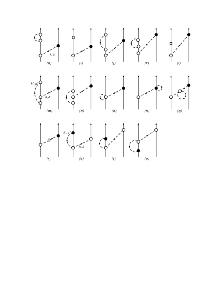
Figure 2: Diagrams contributing to the OPE potential up to order $Q^{2}$ (notation as in Fig. 1). Only a subset of the possible time-ordered diagrams is shown.

Diagrams contributing to the PV potential are shown in Figs. 1 and 2—the diagrams reported in this latter figure contribute to the renormalization of the LEC $h^{1}_{\pi}$. An analysis of the $\pi NN$ vertex corrections was already carried out in Ref. Zhu01 (in that paper the choice $\alpha=1/6$ in Eq. (1) was adopted), and we have verified that we obtain identical expressions to those reported in that work. Contributions given by the various diagrams are reported in Appendix G. In this section, we only list the final expression for the PV potential $V^{(CM)}_{PV}$ as (the dependence on the momenta ${\bm{k}}$ and ${\bm{K}}$ is understood)

$$V^{(CM)}_{PV} = V^{({\rm OPE})}_{PV}+V^{({\rm TPE})}_{PV}$$ (94)

$$+ V^{({\rm RC})}_{PV}+V^{({\rm CT})}_{PV}\ ,$$

namely as a sum of terms due to one-pion exchange (OPE), two-pion exchange (TPE), relativistic corrections (RC), and contact contributions (CT). Following the discussion reported in Appendix G, the OPE term collects i) the non-relativistic (NR) LO contribution $V^{(-1)}({\rm NR})$ of diagram (a) in Fig. 1, namely

$$V^{(-1)}({\rm NR})={g_{A}h^{1}_{\pi}\over 2\sqrt{2}f_{\pi}}\,(\vec{\tau}_{1}\times\vec{\tau}_{2})_{z}\;{i\,{\bm{k}}\cdot({\bm{\sigma}}_{1}+{\bm{\sigma}}_{2})\over\omega_{k}^{2}}\ ,$$ (95)

where $\omega_{k}^{2}=k^{2}+m_{\pi}^{2}$, ii) part of the contribution due to the order $Q^{2}$ pion-nucleon interactions given in Eq. (262) (the term proportional to $V^{(-1)}({\rm NR})$), and iii) the various contributions coming from the diagrams shown in Fig. 2, explicitly

$$V^{({\rm OPE})}_{PV} = V^{(-1)}({\rm NR})\biggl{[}1+{2\,m_{\pi}^{2}\over g_{A}}\,(2\,d_{16}-d_{18})$$ (96)

$$-{8\sqrt{2}\,m^{2}_{\pi}\over h^{1}_{\pi}f_{\pi}^{2}}\,(h^{1}_{2}-h^{1}_{3})-{2\over 3}{g^{2}_{A}\over f^{2}_{\pi}}J_{13}$$

$$-{20\,\alpha-1\over 4f_{\pi}^{2}}J_{01}-2\,\ell_{4}{m^{2}_{\pi}\over f^{2}_{\pi}}$$

$$-{1-10\,\alpha\over 2f_{\pi}^{2}}J_{01}+{1\over 4f_{\pi}^{2}}J_{01}\biggr{]}\ ,$$

where the (infinite) constants $J_{nm}$ are

$$J_{mn}=\int\frac{{\rm d}{\bm{k}}}{(2\pi)^{3}}\,{k^{2m}\over\omega_{k}^{n}}\ .$$ (97)

In the expression above there is a term proportional to $(m_{\pi}/M)^{2}$ coming from $V^{(1)}({\rm RC})$ which we ignore for simplicity—see Appendix G and Eq. (261) for more details on its origin. Note the cancellation of the terms proportional to $J_{01}$, which removes the dependence on $\alpha$. The renormalized OPE potential reads

$$V^{({\rm OPE})}_{PV}={\overline{g}_{A}\overline{h}^{1}_{\pi}\over 2\sqrt{2}\;\overline{f}_{\pi}}(\vec{\tau}_{1}\times\vec{\tau}_{2})_{z}\;{i\,{\bm{k}}\cdot({\bm{\sigma}}_{1}+{\bm{\sigma}}_{2})\over\omega_{k}^{2}}$$ (98)

where

$${\overline{g}_{A}\overline{h}^{1}_{\pi}\over 2\sqrt{2}\;\overline{f}_{\pi}} = {g_{A}h^{1}_{\pi}\over 2\sqrt{2}f_{\pi}}\biggl{[}1+{2\,m_{\pi}^{2}\over g_{A}}(2\,d_{16}-d_{18})$$ (99)

$$-{8\sqrt{2}\,m^{2}_{\pi}\over h^{1}_{\pi}f_{\pi}^{2}}(h^{1}_{2}-h^{1}_{3})-{2\over 3}{g^{2}_{A}\over f^{2}_{\pi}}J_{13}$$

$$-2\,\ell_{4}{m^{2}_{\pi}\over f^{2}_{\pi}}\biggr{]}\ .$$

Here the overlined quantities are the renormalized coupling constants (up to corrections of order $Q^{2}$). Performing a similar analysis for the PC OPE potential, we find (see also Ref. Epel03 ):

$$V^{({\rm OPE})}_{PC} = V^{({\rm OPE},0)}_{PC}\biggl{[}1-{2\over 3}{g^{2}_{A}\over f^{2}_{\pi}}J_{13}$$ (100)

$$+{4\,m_{\pi}^{2}\over g_{A}}(2\,d_{16}-d_{18})-2\,\ell_{4}{m_{\pi}^{2}\over f_{\pi}^{2}}\biggr{]}\ ,$$

where

$$V^{({\rm OPE},0)}_{PC}=-{g^{2}_{A}\over 4f^{2}_{\pi}}\vec{\tau}_{1}\cdot\vec{\tau}_{2}\,{{\bm{\sigma}}_{1}\cdot{\bm{k}}\,\,{\bm{\sigma}}_{2}\cdot{\bm{k}}\over\omega_{k}^{2}}\ ,$$ (101)

is the PC OPE potential at order $Q^{0}$. As usual Epel03 , the singular part coming from $J_{13}$ is absorbed by the LEC’s $d_{16}$ and $\ell_{4}$. The LEC $d_{18}$ is assumed to have only a finite part fixed by the Goldberger-Treiman anomaly. In summary, the PC OPE potential up to order $Q^{2}$ is written as

$$V^{({\rm OPE})}_{PC} = -{\overline{g}_{A}^{2}\over 4\,\overline{f}^{2}_{\pi}}\left(1-{4\,m_{\pi}^{2}\,d_{18}\over g_{A}}\right)$$ (102)

$$\times\,\vec{\tau}_{1}\cdot\vec{\tau}_{2}\,{{\bm{\sigma}}_{1}\cdot{\bm{k}}\ \,\,{\bm{\sigma}}_{2}\cdot{\bm{k}}\over\omega_{k}^{2}}\ ,$$

where the renormalized ratio $\overline{g}_{A}/\overline{f}_{\pi}$ is given by

$${\overline{g}_{A}\over\overline{f}_{\pi}} = {g_{A}\over f_{\pi}}\biggl{(}1-{1\over 3}{g^{2}_{A}\over f^{2}_{\pi}}J_{13}+{4\,m_{\pi}^{2}\over g_{A}}d_{16}-\ell_{4}{m_{\pi}^{2}\over f_{\pi}^{2}}\biggr{)}\ .$$ (103)

In the right-hand side of Eqs. (99), (102) and (103), $g_{A}$ and $f_{\pi}$ can be replaced by the renormalized (physical) values $\overline{g}_{A}$ and $\overline{f}_{\pi}$, which is correct at this order. The constant $J_{13}$ is given in dimensional regularization in Eq. (B38) of Ref. Pastore09 ,

$$J_{13}={3m^{2}_{\pi}\over 8\pi^{2}}(d_{\epsilon}+1)\ ,\quad d_{\epsilon}=-{2\over\epsilon}+\gamma-\ln 4\pi+\ln\left({m^{2}_{\pi}\over\mu^{2}}\right)-{4\over 3}\ ,$$ (104)

where $\gamma\approx 0.5772\cdots$, $\epsilon=3-d$, $d$ being the number of dimensions ($d\rightarrow 3$), and $\mu$ a renormalization scale. Absorbing $d_{\epsilon}$ in both $d_{16}$ and $\ell_{4}$, we have

$${\overline{g}_{A}\over\overline{f}_{\pi}}={g_{A}\over f_{\pi}}\biggl{(}1-{g_{A}^{2}\over f^{2}_{\pi}}\,{m_{\pi}^{2}\over 8\,\pi^{2}}+{4\,m_{\pi}^{2}\over g_{A}}\,\overline{d}_{16}-\overline{\ell}_{4}\,{m_{\pi}^{2}\over f_{\pi}^{2}}\biggr{)}\ ,$$ (105)

where $\overline{d}_{16}$ and $\overline{\ell}_{4}$ are the finite parts of the two corresponding LEC’s. This expression coincides with Eq. (2.44) of Ref. Epel03 , but for a factor 2 in the second term on the r.h.s. of the above equation. However, this difference is of no import, since the final result depends on quantities absorbed in the LEC’s $d_{16}$ and $\ell_{4}$ (namely, on the definition of $d_{\epsilon}$).

Using Eq. (103) for the renormalized (at order $Q^{2}$) ratio $\overline{g}_{A}/\overline{f}_{\pi}$, we can extract from Eq. (99) the expression of the renormalized coupling constant $h^{1}_{\pi}$:

$$\overline{h}^{1}_{\pi} = h^{1}_{\pi}\biggl{[}1-{1\over 3}{g^{2}_{A}\over f^{2}_{\pi}}J_{13}-{2\,m_{\pi}^{2}\over g_{A}}d_{18}-\ell_{4}{m_{\pi}^{2}\over f_{\pi}^{2}}$$ (106)

$$-{8\sqrt{2}\,m^{2}_{\pi}\over h^{1}_{\pi}f_{\pi}^{2}}(h^{1}_{2}-h^{1}_{3})\biggr{]}\ ,$$

and the infinite part coming from $J_{13}$ can be reabsorbed by $\ell_{4}$, $h^{1}_{2}$, and $h^{1}_{3}$.

The potential $V^{({\rm TPE})}_{PV}$ comes from the regular contributions of panels (d)-(g) of Fig. 1 reported in Eqs. (264) and  (269),

$$V^{({\rm TPE})}_{PV}\! = \!-{g_{A}h^{1}_{\pi}\over 2\sqrt{2}f_{\pi}\Lambda_{\chi}^{2}}(\vec{\tau}_{1}\times\vec{\tau}_{2})_{z}\,i\,{\bm{k}}\cdot({\bm{\sigma}}_{1}+{\bm{\sigma}}_{2})\;L(k)$$ (107)

$$-{g_{A}h^{1}_{\pi}\over 2\sqrt{2}f_{\pi}}\,{g_{A}^{2}\over\Lambda_{\chi}^{2}}\biggl{[}4\,\left(\tau_{1z}+\tau_{2z}\right)\,i\,{\bm{k}}\cdot({\bm{\sigma}}_{1}\times{\bm{\sigma}}_{2})\;L(k)$$

$$\qquad\qquad+(\vec{\tau}_{1}\times\vec{\tau}_{2})_{z}\,i\,{\bm{k}}\cdot({\bm{\sigma}}_{1}+{\bm{\sigma}}_{2})$$

$$\qquad\qquad\times\bigl{[}H(k)-3\,L(k)\bigr{]}\biggr{]}\ ,$$

where the loop functions $L(k)$ and $H(k)$ are defined in Eqs. (265) and (270). The TPE potential reported above is in agreement with the expression derived in Refs. Zhu05 ; Liu07 ; Desp08 ; Vries13 . In this and following ${\rm N2LO}$ terms of the potential, the coupling constants $g_{A}$, $f_{\pi}$, and $h^{1}_{\pi}$ can be replaced by the corresponding physical (renormalized) values.

The potential $V^{({\rm RC})}_{PV}$ coincides, except for the term proportional to $k^{2}$ which is reabsorbed in the OPE (as discussed above) and CT (see below) parts, with the quantity $V^{(1)}({\rm RC})$ given in Eq. (261), namely

$$V^{({\rm RC})}_{PV} = {g_{A}h^{1}_{\pi}\over 2\sqrt{2}f_{\pi}}\,{1\over 4\,M^{2}}(\vec{\tau}_{1}\times\vec{\tau}_{2})_{z}\;{1\over\omega_{k}^{2}}$$ (108)

$$\times\,\bigl{[}-4\,i\,K^{2}\,{\bm{k}}\cdot({\bm{\sigma}}_{1}+{\bm{\sigma}}_{2})$$

$$\quad+\,{\bm{k}}\cdot{\bm{\sigma}}_{1}\;({\bm{k}}\times{\bm{K}})\cdot{\bm{\sigma}}_{2}$$

$$\quad+\,{\bm{k}}\cdot{\bm{\sigma}}_{2}\;({\bm{k}}\times{\bm{K}})\cdot{\bm{\sigma}}_{1}\bigr{]}\ .$$

Lastly, the potential $V^{({\rm CT})}_{PV}$, derived from the $4N$ contact diagrams (CT) of Fig. 1, reads

$$V^{({\rm CT})}_{PV} = \frac{1}{\Lambda_{\chi}^{2}f_{\pi}}\Bigl{[}C_{1}\,i\,({\bm{\sigma}}_{1}\times{\bm{\sigma}}_{2})\cdot{\bm{k}}$$ (109)

$$+C_{2}\,\vec{\tau}_{1}\cdot\vec{\tau}_{2}\,i\,({\bm{\sigma}}_{1}\times{\bm{\sigma}}_{2})\cdot{\bm{k}}$$

$$+\overline{C_{3}}\,(\vec{\tau}_{1}\times\vec{\tau}_{2})_{z}\,i\,({\bm{\sigma}}_{1}+{\bm{\sigma}}_{2})\cdot{\bm{k}}$$

$$+\overline{C_{4}}\,(\tau_{1z}+\tau_{2z})\,i\,({\bm{\sigma}}_{1}\times{\bm{\sigma}}_{2})\cdot{\bm{k}}$$

$$+C_{5}\,{\cal I}^{ab}\,\tau_{1a}\,\tau_{2b}\,i\,({\bm{\sigma}}_{1}\times{\bm{\sigma}}_{2})\cdot{\bm{k}}\Bigr{]}\ ,$$

where the $\overline{C_{i}}$ are the renormalized LEC’s, in which the infinite constants coming from the evaluation (in dimensional regularization) of the TPE diagrams—the terms given in Eqs. (266) and (271)—as well as the contribution proportional to $\omega_{k}^{2}$ in Eq. (261) and the contribution proportional to $h^{1}_{12}$ in Eq. (262) have been reabsorbed (see Appendix G.2 for more details).

In the applications discussed in Sec. IV, the configuration-space version of the potential is needed. This formally follows from

$$\!\!\!\!\!\!\!\!\!\!\!\!\langle{\bm{r}}_{1}^{\prime}{\bm{r}}_{2}^{\prime}|V|{\bm{r}}_{1}{\bm{r}}_{2}\rangle = \delta({\bm{R}}-{\bm{R}}^{\prime})\int{d^{3}k\over(2\pi)^{3}}{d^{3}K\over(2\pi)^{3}}$$ (110)

$$\times e^{i({\bm{K}}+{\bm{k}}/2)\cdot{\bm{r}}^{\prime}}V({\bm{k}},{\bm{K}})e^{-i({\bm{K}}-{\bm{k}}/2)\cdot{\bm{r}}}\ ,$$

where ${\bm{r}}={\bm{r}}_{1}-{\bm{r}}_{2}$ and ${\bm{R}}=({\bm{r}}_{1}+{\bm{r}}_{2})/2$, and similarly for the primed variables. In order to carry out the Fourier transforms above, the integrand is regularized by including a cutoff of the form

$$C_{\Lambda}(k)={\rm e}^{-(k/\Lambda)^{4}}\ ,$$ (111)

where the cutoff parameter $\Lambda$ is taken in the range 500–600 MeV. With such a choice the OPE, TPE, and CT components of the resulting potential are local, i.e., $\langle{\bm{r}}_{1}^{\prime}{\bm{r}}_{2}^{\prime}|V|{\bm{r}}_{1}{\bm{r}}_{2}\rangle=\delta({\bm{R}}-{\bm{R}}^{\prime})\,\delta({\bm{r}}-{\bm{r}}^{\prime})V({\bm{r}})$, while the RC component contains mild non-localities associated with linear and quadratic terms in the relative momentum operator $-i{\bm{\nabla}}$. Explicit expressions for all these components are listed in Appendix H.

IV Results

In this section, we report results for PV observables in the $A$=2–4 systems. The $A$=2 calculations are based on the (weak interaction) PV $NN$ potential derived in the previous section (and summarized in Appendix H) and on the (strong interaction) PC $NN$ potential obtained by Entem and Machleidt EM03 ; ME11 at next-to-next-to-next-to-leading order (N3LO). This potential is regularized with a cutoff function depending on a parameter $\Lambda$—its functional form, however, is different from that adopted here for $V_{PV}$. Below we consider the two versions corresponding to $\Lambda$=500 MeV and $\Lambda$=600 MeV, labeled N3LO-500 and N3LO-600, respectively. The $A$=3 and 4 calculations also include a (strong interaction) PC three-nucleon ($NNN$) potential derived in $\chi$EFT at ${\rm N2LO}$ Eea02 . It too depends on a cutoff parameter $\Lambda$, and here we use values for it which are consistent with those in the PC and PV $NN$ potentials. These three-nucleon potentials, labeled, respectively, N2LO-500 and N2LO-600, depend in addition on two unknown LEC’s, denoted as $c_{D}$ and $c_{E}$. In this work, they have been determined by reproducing the $A$=3 binding energies and the Gamow-Teller matrix element in tritium $\beta$-decay Gazit ; Mea12 . Their values are listed in Table 1.

Table 1: The $NN$ and $NNN$ chiral potentials used in this work. In columns 2–4 the values for the cutoff parameter $\Lambda$ (in MeV) and adimensional coefficients $c_{D}$ and $c_{E}$ in the $NNN$ potential are listed. In the last column the binding energies predicted for ${{}^{4}{\rm He}}$ are reported corresponding to the two sets.

PC interactions	$\Lambda$	$c_{D}$	$c_{E}$	B$({{}^{4}{\rm He}})$
	[MeV]			[MeV]
N3LO/N2LO-500	$500$	$-0.12$	$-0.196$	$28.49$
N3LO/N2LO-600	$600$	$-0.26$	$-0.846$	$28.64$

The final expression of the potential is given in Eq. (277). The component $V^{({\rm OPE})}$ is the LO term (of order $Q^{-1}$), although the coupling constants contain also contributions from the N2LO (order $Q^{1}$) vertex corrections, while the components RC, TPE, and CT are N2LO terms. In the following, the values $\overline{g}_{A}=1.267$ and $\overline{f}_{\pi}=92.4$ MeV are adopted.

This section is organized as follows. In Sec. IV.1, we provide estimates for the renormalized LEC’s $h^{1}_{\pi}$ and $C_{i}$ (with the overline omitted for brevity) entering the PV potential, using a resonance saturation model, in practice by exploiting what is known about the DDH parameters DDH . In Sec. IV.2, we provide constraints for some of the LEC’s by fitting currently available measurements of the $\vec{p}$-$p$ longitudinal asymmetry. In Secs. IV.3 and IV.4 we present a study of, respectively, spin-rotation effects in $n$-$p$ and $n$-$d$ scattering, and of the longitudinal asymmetry in the ³He($\vec{n},p$)³H reaction.

IV.1 Estimates of the LEC’s

In Ref. DDH the pion-nucleon PV coupling constant $h^{1}_{\pi}$ was estimated to vary in the “reasonable range” $0\leq h_{\pi}^{1}\leq 11.4\times 10^{-7}$ with the “best value” $h_{\pi}^{1}=4.56\times 10^{-7}$. More recently, a lattice calculation has estimated $h_{\pi}^{1}\approx 1\times 10^{-7}$ Wasem2012 . Therefore, in the following we perform calculations for three values of $h^{1}_{\pi}$:

1. $h_{\pi}^{1}=1\times 10^{-7}$ (lattice estimate);

2. $h_{\pi}^{1}=4.56\times 10^{-7}$ (DDH “best value”);

3. $h_{\pi}^{1}=11.4\times 10^{-7}$ (maximum value allowed in the DDH “reasonable range”).

In order to estimate the LEC’s $C_{i}$ in $V^{({\rm CT})}_{PV}$, we match the components of the DDH potential mediated by $\rho$ and $\omega$ exchanges to those of $V^{({\rm CT})}_{PV}$, and obtain in the limit $k\ll m_{\rho}$, $m_{\omega}$:

$$C^{({\rm DDH})}_{1} = -{3\over 2}g_{\rho}h^{0}_{\rho}D_{\rho}-{3\over 2}g_{\omega}h^{0}_{\omega}D_{\omega}\ ,$$ (112)

$$C^{({\rm DDH})}_{2} = -g_{\rho}h^{0}_{\rho}\left({1\over 2}+\kappa_{\rho}\right)D_{\rho}-{1\over 2}g_{\omega}h^{0}_{\omega}D_{\omega}\ ,$$ (113)

$$C^{({\rm DDH})}_{3} = -{1\over 2}g_{\rho}(h^{1^{\prime}}_{\rho}-h^{1}_{\rho})D_{\rho}-{1\over 2}g_{\omega}h^{1}_{\omega}D_{\omega}$$ (114)

$$C^{({\rm DDH})}_{4} = -{1\over 2}g_{\rho}h^{1}_{\rho}(2+\kappa_{\rho})D_{\rho}-g_{\omega}h^{1}_{\omega}D_{\omega}\ ,$$ (115)

$$C^{({\rm DDH})}_{5} = -{1\over 2\sqrt{6}}g_{\rho}h^{2}_{\rho}(2+\kappa_{\rho})D_{\rho}\ ,$$ (116)

where $g_{\rho}$, $\kappa_{\rho}$, $g_{\omega}$, $h^{0,1,2,1^{\prime}}_{\rho}$, and $h^{0,1}_{\omega}$ are the vector-meson coupling constants in the DDH potential, and

$$D_{\rho} = {\Lambda^{2}_{\chi}\over m^{2}_{\rho}}\,{f_{\pi}\over M}\left(1-{m_{\rho}^{2}\over\Lambda_{\rho}^{2}}\right)^{2}\ ,$$ (117)

$$D_{\omega} = {\Lambda^{2}_{\chi}\over m^{2}_{\omega}}\,{f_{\pi}\over M}\left(1-{m_{\omega}^{2}\over\Lambda_{\omega}^{2}}\right)^{2}\ .$$ (118)

The cutoff parameters $\Lambda_{\rho}$ and $\Lambda_{\omega}$ enter the vector-meson hadronic form factors used to regularize the behavior of the associated components of the DDH potential at large momenta (the values adopted here $\Lambda_{\rho}$=1.31 GeV and $\Lambda_{\omega}$=1.50 GeV are from the one-boson-exchange charge-dependent Bonn potential Machleidt01 ).

In the original work DDH “best values” and “reasonable ranges”, derived from a quark model and symmetry arguments, were proposed also for the DDH vector-meson PV coupling constants. In particular, the analysis of Ref. H81 suggested that the coupling constant $h^{1^{\prime}}_{\rho}$ is quite small. In subsequent years, there were several studies attempting to estimate the values of these coupling constants either from theoretical models DZ86 ; Feldman1991 or from comparisons between predictions for PV observables and available experimental data. For example, in Ref. Carlson02 constraints on the DDH PV vector-meson coupling constants were obtained by fitting data on the $\vec{p}\,$-$p$ longitudinal asymmetry (see below). In a later paper Schiavilla04 these constraints and “best value” estimates—in particular, the value $h^{1}_{\pi}=4.56\times 10^{-7}$ was assumed—resulted in a DDH model, denoted as “DDH-adj” Schiavilla04 . From the DDH-adj set of vector-meson PV coupling constants we find via Eqs. (112)–(116), in units of $10^{-7}$,

$$C^{({\rm DDH})}_{1}\approx 1\ ,\quad C^{({\rm DDH})}_{2}\approx+30\ ,\quad C^{({\rm DDH})}_{3}\approx-2\ ,$$

$$C^{({\rm DDH})}_{4}\approx 0\ ,\quad C^{({\rm DDH})}_{5}\approx+7\ .$$ (119)

The large value of $C^{({\rm DDH})}_{2}$ is due to the tensor coupling constant $\kappa_{\rho}$=6.1 of the $\rho$-meson to the nucleon in Ref. Machleidt01 . Clearly, these values should be taken only as indicative, since terms in the DDH vector-meson potential implicitly also account for TPE components, which in the $\chi$EFT PV potential are included explicitly.

IV.2 The $\vec{p}\,$-$p$ longitudinal asymmetry

There exist three accurate measurements of the angle-averaged $\vec{p}\,$-$p$ longitudinal asymmetry $\overline{A}^{\,pp}_{z}(E)$, obtained at different laboratory energies $E$ Eversheim91 ; Kistryn87 ; Berdoz03 :

$$\overline{A}_{z}^{\,pp}(13.6{\rm MeV})=(-0.97\pm 0.20)\times 10^{-7}\ ,$$

$$\overline{A}_{z}^{\,pp}(45{\rm MeV})=(-1.53\pm 0.21)\times 10^{-7}\ ,$$ (120)

$$\overline{A}_{z}^{\,pp}(221{\rm MeV})=(+0.84\pm 0.34)\times 10^{-7}\ .$$

These data points have been obtained by combining results from various measurements, as discussed in Sec. IV of Ref. Carlson02 . The errors reported above include both statistical and systematic errors added in quadrature. These experiments measure the asymmetry averaged over a range $(\theta_{1},\theta_{2})$ of (laboratory) scattering angles.

The calculation of this observable was carried out with the methods of Ref. Carlson02 . We have explicitly verified that the angular distribution of the longitudinal asymmetry $A_{z}(E,\theta)$ is approximately constant except at small angles $\lesssim 15$ deg, where Coulomb scattering dominates. In the following, we have computed the average asymmetry $\overline{A}^{\,pp}_{z}(E)$ using for $E=13.6$ MeV $(\theta_{1},\theta_{2})=(20,78)$ deg, for $E=45$ MeV $(\theta_{1},\theta_{2})=(23,52)$ deg, and for $E=221$ MeV $(\theta_{1},\theta_{2})=(5,90)$ deg.

For $pp$ scattering it is easily seen that the longitudinal asymmetry can be expressed as

$$\overline{A}_{z}^{\,pp}(E)=a^{(pp)}_{0}(E)\,h^{1}_{\pi}+a^{(pp)}_{1}(E)\,C\ ,$$ (121)

where

$$C=C_{1}+C_{2}+2\,(C_{4}+C_{5})\ ,$$ (122)

and $a^{(pp)}_{0}(E)$ and $a^{(pp)}_{1}(E)$ are numerical coefficients independent of the LEC values (however, they do depend on the cutoff $\Lambda$ in the PC and PV chiral potentials). The dependence of $\overline{A}^{\,pp}_{z}(E)$ on $h^{1}_{\pi}$ is due to TPE components in the PV potential. The coefficients calculated using the PC and PV $NN$ potentials for the two choices of cutoff parameters are reported in Table 2. As is well known, the values of $a^{(pp)}_{i}$ at low energy scale as $\sqrt{E}$, since the energy dependence of the longitudinal asymmetry in this energy range is driven by that of the S-wave (strong interaction) phase shift Carlson02 . Because of this scaling, the experimental points at $E$=13.6 MeV and 45 MeV do not provide independent constraints on the LEC’s $h^{1}_{\pi}$ and $C$.

$E$ [MeV]	$a^{(pp)}_{0}$	$a^{(pp)}_{1}$
$\Lambda=500$ MeV
$13.6$	${\phantom{-}}0.26992$	$-0.04159$
$45$	${\phantom{-}}0.55528$	$-0.07994$
$221$	$-0.24337$	${\phantom{-}}0.03134$
$\Lambda=600$ MeV
$13.6$	${\phantom{-}}0.25441$	$-0.03990$
$45$	${\phantom{-}}0.53438$	$-0.07841$
$221$	$-0.19341$	${\phantom{-}}0.02743$

Table 2: Values of the coefficients $a^{(pp)}_{i}(E)$ at the three energies corresponding to the experimental data points for the two choices of cutoff parameters $\Lambda$. The calculations include contributions up to $J_{\rm max}=6$ in the partial-wave expansion of the $pp$ scattering state.

If we assume $h^{1}_{\pi}$=4.56 $\times 10^{-7}$ and $\Lambda$=500 MeV, we obtain $C\approx 50\times 10^{-7}$ by fitting the experimental value at $E$=13.6 MeV, in agreement with the result of Ref. Vries13 (note that the operator proportional to the LEC $C$ used in that work has a minus sign relative to that defined here). In order to take into account experimental uncertainties, we have performed a $\chi^{2}$ analysis, and in Fig. 3 we report the $h^{1}_{\pi}$ and $C$ values for which $\chi^{2}=2$ when the cutoff in the PC and PV chiral potentials is fixed at either $\Lambda$=500 or $\Lambda$=600 MeV. The resulting two elliptic regions almost coincide, and there appears to be a strong correlation between $h^{1}_{\pi}$ and $C$. The range of allowed $h^{1}_{\pi}$ values is rather large $-1\times 10^{-6}<h^{1}_{\pi}<2\times 10^{-6}$, containing the whole DDH “reasonable range”. Note that the two ellipses are rather narrow and almost coincident with a straight line. These conclusions are the same as those derived in a similar analysis by the authors of Ref. Vries13 .

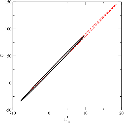
Figure 3: (color online). Contours of $h^{1}_{\pi}$ and $C$ values (in units of $10^{-7}$) corresponding to which $\chi^{2}=2$ for the $\vec{p}\,$-$p$ longitudinal asymmetry. The black solid (red dashed) contour is relative to $\Lambda$=500 (600) MeV.

In Table 3, we report representative values of $C$, determined from Fig. 3, corresponding to the three choices of $h^{1}_{\pi}$ discussed in the previous section. These values are used in the following sections to provide estimates for PV observables in $A$=2–4 systems.

$\Lambda$ [MeV]	$\qquad h_{\pi}^{1}\quad$	$\quad C\qquad$
	$1\phantom{.00}$	$26.7$
500	$4.56$	$51.5$
	$11.4$	$99.2$
	$1\phantom{.00}$	$27.6$
600	$4.56$	$51.4$
	$11.4$	$97.2$

Table 3: Values for $C$ corresponding to different values of $h^{1}_{\pi}$ (both in units of $10^{-7}$) and $\Lambda$, as determined from Fig. 3. The $C$ values are those lying on the major axis of the elliptical contours.

IV.3 $\vec{n}$-$p$ and $\vec{n}$-$d$ spin rotations

The rotation of the neutron spin in a plane transverse to the beam direction induced by PV components in the $NN$ potential is given by

$$\frac{{\rm d}\phi^{(nX)}}{{\rm d}z} = \frac{2\pi\rho}{(2S_{X}+1)\,v_{\rm rel}}{\rm Re}\!\sum_{m_{n}m_{X}}\epsilon_{m_{n}}$$ (123)

$$\times \!{}^{(-)}\langle p\hat{\bf z};m_{n},m_{X}|V_{PV}|p\hat{\bf z};m_{n},m_{X}\rangle^{(+)}\ ,$$

where $\rho$ is the density of hydrogen or deuterium nuclei for $X$=$p$ or $d$, $V_{PV}$ denotes the PV potential, $\mid\!p\hat{\bf z};m_{n},m_{X}\rangle^{(\pm)}$ are the $n$-$X$ scattering states with outgoing-wave $(+)$ and incoming-wave $(-)$ boundary conditions and relative momentum ${\bf p}=p\,\hat{\bf z}$ taken along the spin-quantization axis (the $\hat{\bf z}$-axis), $S_{X}$ is the $X$ spin, and $v_{\rm rel}=p/\mu$ is the magnitude of the relative velocity, $\mu$ being the $n$-$X$ reduced mass. The expression above is averaged over the spin projections $m_{X}$; however, the phase factor $\epsilon_{m_{n}}=(-)^{1/2-m_{n}}$ is $\pm 1$ depending on whether the neutron has $m_{n}=\pm 1/2$.

We consider the $\vec{n}$-$p$ and $\vec{n}$-$d$ spin rotations for vanishing incident neutron energy (measurements of this observable are performed using ultra-cold neutron beams). In the following, we assume $\rho=0.4\times 10^{23}$ cm^-3. The $n$-$d$ wave functions have been obtained with the hyperspherical-harmonics (HH) method Kea08 ; Mea09 from the Hamiltonians N3LO/N2LO-500 and N3LO/N2LO-600 of Sec. IV. Details of the calculation of ${\rm d}\phi/{\rm d}z$ for $\vec{n}$-$p$ and $\vec{n}$-$d$ can be found in Refs. Schiavilla04 and Schiavilla08 ; Song11 , respectively. In general, the rotation angle depends linearly on the PV LEC’s:

$$\frac{{\rm d}\phi^{(nX)}}{{\rm d}z} = h^{1}_{\pi}\,b_{0}^{(nX)}+C_{1}\,b_{1}^{(nX)}+C_{2}\,b_{2}^{(nX)}$$ (124)

$$+\,C_{3}\,b_{3}^{(nX)}+C_{4}\,b_{4}^{(nX)}+C_{5}\,b_{5}^{(nX)}\ ,$$

where the $b_{i}^{(nX)}$ for $i=0,\ldots,5$ are numerical coefficients. Their calculated values for the two choices of cutoff $\Lambda$ are listed in Table 4.

$\vec{n}$-$p$ scattering
$\Lambda$ [MeV]	$b^{(np)}_{0}$	$b^{(np)}_{1}$	$b^{(np)}_{2}$	$b^{(np)}_{3}$	$b^{(np)}_{4}$	$b^{(np)}_{5}$
500	$1.35997$	$0.24399$	$0.17390$	$0.10537$	$0.00000$	$-0.90585$
600	$1.26392$	$0.23540$	$0.15839$	$0.08483$	$0.00000$	$-0.86459$
$\vec{n}$-$d$ scattering
$\Lambda$ [MeV]	$b^{(nd)}_{0}$	$b^{(nd)}_{1}$	$b^{(nd)}_{2}$	$b^{(nd)}_{3}$	$b^{(nd)}_{4}$	$b^{(nd)}_{5}$
500	$2.17913$	$-0.01046$	$-0.15997$	$0.19117$	$0.06367$	$0.00032$
600	$2.22165$	$-0.00684$	$-0.18226$	$0.18232$	$0.06750$	$0.00030$

Table 4: Values of the coefficients $b^{(nX)}_{i}$ in units of Rad m^-1 for the $\vec{n}$-$p$ and $\vec{n}$-$d$ spin rotations calculated for the two choices of cutoff $\Lambda$ at vanishing neutron beam energy.

The coefficient $b^{(nX)}_{0}$ receives contributions from the OPE, TPE, and RC components of the PV potential, see Eq. (94). For example, for $\vec{n}$-$p$ scattering and the N3LO-500 PC potential we find $b^{(np)}_{0}=1.23759({\rm OPE})+0.13441({\rm TPE})-0.01202({\rm RC})=1.35997$ Rad m^-1, so the TPE (RC) contribution is about 10 (1)% of the OPE. Inspection of Table 4 also shows that the $\vec{n}$-$p$ spin rotation is sensitive to all LEC’s except $C_{4}$ (proportional to $\tau_{1z}+\tau_{2z}$); in particular, there is a large sensitivity to $C_{5}$, which multiplies the isotensor term of the PV potential.

The $\vec{n}$-$p$ spin rotation was already studied in Ref. Liu07 using the same PV potential as in the present work but the Argonne $v_{18}$ (AV18) PC potential AV18 . The results obtained in this work cannot be directly compared with those reported in Ref. Liu07 because of differences in the definition of the LEC’s, in the value of the cutoff, and in the presentation of the results themselves. In Ref. Liu07 the CT component of the PV potential has a redundant parametrization in terms of 10 LEC’s. By expressing the 5 CT operators depending on ${\bm{K}}$ in terms of those which only depend on ${\bm{k}}$ via Eqs. (25), (26) and (29) of Ref. Liu07 , we obtain (in units of Rad m^-1)

$$\frac{{\rm d}\phi^{(np)}}{{\rm d}z}|_{\rm Liu} \approx \Bigl{[}1.15\,(h^{1}_{\pi})_{\rm OPE}-0.13\,(h^{1}_{\pi})_{\rm TPE}$$ (125)

$$+0.15\,C_{1}+0.12\,C_{2}$$

$$+0.08\,C_{3}-0.56\,C_{5}\Bigr{]}\ .$$

The coefficients multiplying the various LEC’s can be compared with the $b^{(np)}_{i}$ reported in Table 4. There is qualitative agreement, given that the coefficients above correspond to the AV18 model as well as to a larger cutoff $\Lambda$ in the PV potential than adopted here. In Eq. (125), the factors multiplying $(h^{1}_{\pi})_{\rm OPE}$ and $(h^{1}_{\pi})_{\rm TPE}$ are the contributions to $b_{0}^{(np)}$ from the OPE and TPE components (of the PV potential), respectively. These should be compared to the OPE and TPE results, obtained here (see above): 1.23759 Rad m^-1 and 0.13441 Rad m^-1. In the present case, the TPE contribution is positive and increases $b^{(np)}_{0}$. We have verified that this contribution is very sensitive to the cutoff parameter $\Lambda$. For example, using $\Lambda=1.3$ GeV as in Ref. Liu07 , we find that the TPE contribution becomes negative.

	$\Lambda=500$ MeV			$\Lambda=600$ MeV
LEC	I	II	III	I	II	III
$h_{\pi}^{1}$	$\phantom{0}1.0$	$\phantom{0}4.56$	$11.4$	$\phantom{0}1.0$	$\phantom{0}4.56$	$11.4$
$C_{2}$	$13.7$	$28.5\phantom{0}$	$56.2$	$14.6$	$28.4\phantom{0}$	$54.2$
$C_{5}$	$\phantom{0}5.0$	$10.0\phantom{0}$	$20.0$	$\phantom{0}5.0$	$10.0\phantom{0}$	$20.0$

Table 5: Values for the LEC’s $h_{\pi}^{1}$, $C_{2}$, and $C_{5}$ correspoding to sets I, II, and III (see text). The remaining LEC’s are taken to have the values $C_{1}=1$, $C_{3}=-1$, and $C_{4}=1$ in each set. All LEC’s are in units of $10^{-7}$.

In reference to the $\vec{n}$-$d$ spin rotation, we note the large sensitivity to $h^{1}_{\pi}$ (this fact is well known Schiavilla08 ; Song11 ), and to the LEC’s $C_{2}$ and $C_{3}$. A measurement of this observable could be very useful in constraining their values.

In order to provide an estimate for the magnitude of the $\vec{n}$-$p$ and $\vec{n}$-$d$ spin rotations, we proceed as follows. We set $C_{1}=1$, $C_{3}=-1$, and $C_{4}=1$, since estimates from Eq. (119) indicate that they are much smaller (in magnitude) than $C_{2}$ and $C_{5}$. For each set of $h^{1}_{\pi}$ and $\Lambda$ values, the corresponding value of the LEC $C_{5}$ is as reported in Table 5. Finally, the value of the LEC $C_{2}$ is fixed so that the parameter $C$ in Eq. (122) is as given in Table 3. All the LEC values are reported in Table 5. The three sets are denoted hereafter as I, II, and III.

The cumulative contributions to ${\rm d}\phi^{(nX)}/{\rm d}z$ using the LEC’s in Table 5 are reported in Table 6. There is a large sensitivity to $h^{1}_{\pi}$. However, the dependence of the results on $\Lambda$ is also significant, especially in the $\vec{n}-p$ case, presumably due to the fact that the LEC’s $C_{1,3,4,5}$ have been taken to have the same values for the two choices of $\Lambda$. In general, we expect the values of these LEC’s to vary as $\Lambda$ changes. The effect of the RC term in the PV potential is tiny. For the $\vec{n}$-$d$ spin rotation angle, we note that the TPE contribution is at few % level for $\Lambda$=500 MeV, but negligible for $\Lambda$=600 MeV.

	$\Lambda=500$ MeV			$\Lambda=600$ MeV
$\vec{n}$-$p$ spin rotation
	I	II	III	I	II	III
OPE	${\phantom{-}}1.24$	$5.64$	$14.11$	${\phantom{-}}1.19$	$5.42$	$13.56$
TPE	${\phantom{-}}1.37$	$6.26$	$15.64$	${\phantom{-}}1.27$	$5.80$	$14.50$
RC	${\phantom{-}}1.36$	$6.20$	$15.50$	${\phantom{-}}1.26$	$5.76$	$14.41$
CT	$-0.65$	$2.24$	$\phantom{0}7.30$	$-0.60$	$1.77$	$\phantom{0}5.85$
$\vec{n}$-$d$ spin rotation
OPE	${\phantom{-}}2.25$	$10.27$	$25.67$	${\phantom{-}}2.25$	$10.25$	$25.62$
TPE	${\phantom{-}}2.21$	$10.06$	$25.15$	${\phantom{-}}2.25$	$10.26$	$25.64$
RC	${\phantom{-}}2.18$	$\phantom{0}9.94$	$24.84$	${\phantom{-}}2.22$	$10.13$	$25.33$
CT	$-0.15$	$\phantom{0}5.24$	$15.72$	$-0.56$	$\phantom{0}4.84$	$15.33$

Table 6: Cumulative contributions to the $\vec{n}$-$p$ and $\vec{n}$-$d$ spin rotations in units of $10^{-7}$ Rad m^-1, corresponding to sets I, II, and III of LEC’s as specified in Table 5.

IV.4 The ³He($\vec{n},p$)³H longitudinal asymmetry

For ultracold neutrons the longitudinal asymmetry $A_{z}$ for the reaction ³He($\vec{n},p$)³H is given by $A_{z}=a_{z}\,{\rm cos}\,\theta$ Viviani10 , where $\theta$ is the angle between the outgoing proton momentum and the neutron beam direction. The coefficient $a_{z}$ can be expressed in terms of products of $T$-matrix elements involving three PC and three PV transitions (see Ref. Viviani10 for details). These $T$-matrix elements are calculated by means of the HH method Kea08 ; Mea09 , using the PC and PV chiral potentials of the previous sections.

$\Lambda$ [MeV]	$a_{0}$	$a_{1}$	$a_{2}$	$a_{3}$	$a_{4}$	$a_{5}$
500	$-0.1444$	$0.0061$	$0.0226$	$-0.0199$	$-0.0174$	$-0.0005$
600	$-0.1293$	$0.0081$	$0.0320$	$-0.0161$	$-0.0156$	$-0.0001$

Table 7: Values of the coefficients $a_{i}$ entering the ³He($\vec{n},p$)³H longitudinal asymmetry calculated at vanishing neutron beam energy and for two choices of the cutoff parameter $\Lambda$. The calculations are performed summing four-body states up to $J_{\rm max}=1$, namely including S–waves in the incident channel.

The coefficient $a_{z}$ is expressed as

$$a_{z} = a_{0}\,h^{1}_{\pi}+a_{1}\,C_{1}+a_{2}\,C_{2}$$ (126)

$$+a_{3}\,C_{3}+a_{4}\,C_{4}+a_{5}\,C_{5}\ ,$$

and the calculated coefficients $a_{i}$ are listed in Table 7. The largest coefficient is $a_{0}$, while $a_{2}$, $a_{3}$ and $a_{4}$ are of similar magnitude and about a factor 5 smaller than $a_{0}$. The coefficients $a_{1}$ and $a_{5}$ are more than an order of magnitude smaller than the leading $a_{0}$. Naively, one would have expected the dominant contributions to come from the isoscalar terms (proportional to the LEC’s $C_{1}$ and $C_{2}$), since at the low energies of interest here the reaction proceeds mainly through the (close) $0^{+}$ and $0^{-}$ resonances in the ${{}^{4}{\rm He}}$ spectrum, having total isospin $T$=0 TWH92 . However, the Coulomb interaction in the final state induces significant isospin mixing, and the isovector terms in the PV potential end up giving unexpectedly large contributions. In any case, the “isoscalar” coefficient $a_{2}$ when multiplied by $C_{2}$, which is expected to be large, leads to a contribution of similar magnitude as that of $a_{0}\,h^{1}_{\pi}$, but of opposite sign. The destructive interference between these two contributions makes the longitudinal asymmetry rather sensitive to short-range physics and, in particular, to the cutoff $\Lambda$ (see Table 8 below).

	$\Lambda=500$ MeV			$\Lambda=600$ MeV
	I	II	III	I	II	III
OPE	$-0.118$	$-0.537$	$-1.34$	$-0.099$	$-0.453$	$-1.13$
TPE	$-0.147$	$-0.669$	$-1.67$	$-0.131$	$-0.597$	$-1.49$
RC	$-0.144$	$-0.658$	$-1.65$	$-0.129$	$-0.589$	$-1.47$
CT	$\phantom{0}0.171$	$-0.012$	$-0.38$	$\phantom{0}0.346$	$\phantom{0}0.326$	$\phantom{0}0.27$

Table 8: Cumulative contributions to the coefficient $a_{z}$ (in units of $10^{-7}$), describing the ³He($\vec{n},p$)³H longitudinal asymmetry at vanishing neutron beam energy, corresponding to sets I, II, and III of LEC’s as specified in Table 5.

In Table 8 we report cumulatively the contributions of the OPE, TPE, RC, CT components of the PV potential to the parameter $a_{z}$. These predictions for $a_{z}$ correspond to sets I, II, and III of LEC’s, as specified in Table 5. The RC contribution is tiny (at the 1% level), while the TPE contribution is about 30% of the OPE one. Upon including the CT contribution, we observe a large cancellation, particularly effective for small values of $h^{1}_{\pi}$. As already noted, this cancelation comes mostly from the term proportional to the LEC $C_{2}$.

V Conclusions

In this paper we have studied the $\chi$EFT Lagrangian describing PV interactions of nucleons and pions up to order $Q^{2}$. This Lagrangian has been used to derive the PV $NN$ potential at ${\rm N2LO}$. We have also discussed subleading contributions to the OPE component, and carried out the renormalization of the pion-nucleon PV coupling constant $h^{1}_{\pi}$. Finally, we have investigated PV effects in a number of reactions involving few-nucleon systems. We find that (i) the $\vec{p}\,$-$p$ longitudinal asymmetry is sensitive to $h^{1}_{\pi}$ (via the TPE component of the PV potential) and to the combination of LEC’s $C=C_{1}+C_{2}+2\,C_{4}+2\,C_{5}$; (ii) the $\vec{n}$-$p$ spin rotation is sensitive to all LEC’s but $C_{4}$, while the $\vec{n}$-$d$ spin rotation is sensitive to $h^{1}_{\pi}$, $C_{2}$, and $C_{3}$; and (iii) the $n$-${{}^{3}{\rm He}}$ longitudinal asymmetry is sensitive to $h^{1}_{\pi}$, $C_{2}$, $C_{3}$, and $C_{4}$.

At the SNS facility at Oak Ridge National Laboratory a measurement of the PV asymmetry $a_{\gamma}$ in the ¹H$(\vec{n},\gamma)^{2}$H radiative capture is in progress (the NPDGAMMA experiment). This observable is mainly sensitive to $h^{1}_{\pi}$ Desp08 . It is expected that this measurement will provide tight constraints on its value. Once $h^{1}_{\pi}$ is known, measurements of the $\vec{n}$-$p$ and $\vec{n}$-$d$ spin rotations, and of the $\vec{n}-$${{}^{3}{\rm He}}$ longitudinal asymmetry, would provide constraints on the LEC’s $C_{i}$. It would also be very valuable to have new and more precise measurements of the $\vec{p}\,$-$p$ longitudinal asymmetry at different proton energies.

An experiment to measure the $\vec{n}$-${{}^{3}{\rm He}}$ $A_{z}$ asymmetry has already been approved at the SNS facility, and the experimental apparatus is in an advanced stage of construction. The experiment should start taking data after the conclusion of NPDGAMMA. An accurate measurement of $A_{z}$ could lead to a precise determination of $C_{2}$. At the present time, experiments to measure $\vec{n}$-$p$ and $\vec{n}$-$d$ spin rotation angles are not planned, but could provide useful information on $C_{5}$ and $C_{3}$, respectively. The only other experiment in progress we are aware of is a measurement of the $\vec{n}$-${{}^{4}{\rm He}}$ spin rotation at NIST Bass09 .

In the future, we plan to use the $\chi$EFT Lagrangians of order $Q^{2}$ we have derived here to study PV couplings to the electromagnetic field and, in particular, to provide estimates for PV observables in the $np$ and $nd$ radiative captures.

Appendix A Chiral transformation properties of $D_{\mu}X^{a}_{L/R}$

The transformation properties of the quantities $X^{a}_{L/R}$, as already given in Eq. (15), are

$$X^{a}_{R}\to h\;u^{\dagger}\;R^{\dagger}\tau_{a}R\;u\;h^{\dagger}\ ,\quad X^{a}_{L}\to h\;u\;L^{\dagger}\tau_{a}L\;u^{\dagger}\;h^{\dagger}\ ,$$ (127)

i.e., $X^{a}_{R}\to h\bigl{(}X^{a}_{R}\bigr{)}^{({\rm constructed\ with\ }R^{\dagger}\tau_{a}R)}h^{\dagger}$ and similarly for $X^{a}_{L}$. For local transformations, the $SU(2)$ matrices $L$ and $R$ depend on the space-time coordinate $x$, and care must be taken when considering four-gradients of $X^{a}_{L/R}$, since under chiral transformations they contain terms like $h\,u^{\dagger}R^{\dagger}\tau_{a}(\partial_{\mu}R)\,u\,h^{\dagger}$, which transform differently from $X^{a}_{L/R}$. It is convenient to define the following quantities

$$\left(X^{a}_{R}\right)_{\mu} = \left[D_{\mu}+i\,u^{\dagger}r_{\mu}u\,,\,X^{a}_{R}\right]\ ,$$ (128)

$$\left(X^{a}_{L}\right)_{\mu} = \left[D_{\mu}+i\,u\,\ell_{\mu}u^{\dagger}\,,\,X^{a}_{L}\right]\ ,$$ (129)

which explicitly read

$$\!\!\!\!\!\!\!\!\!\!\!\!\left(X^{a}_{R}\right)_{\mu} = \partial_{\mu}(u^{\dagger}\tau_{a}u)+\left[\Gamma_{\mu}\,,\,u^{\dagger}\tau_{a}u\right]+iu^{\dagger}\left[r_{\mu}\,,\,\tau_{a}\right]u\ ,$$ (130)

$$\!\!\!\!\!\!\!\!\!\!\!\!\left(X^{a}_{L}\right)_{\mu} = \partial_{\mu}(u\,\tau_{a}u^{\dagger})+\left[\Gamma_{\mu}\,,\,u\,\tau_{a}u^{\dagger}\right]+iu\,\left[l_{\mu}\,,\,\tau_{a}\right]u^{\dagger}\ .$$ (131)

Then, under chiral transformation it is easily seen that

$$\left(X^{a}_{R}\right)_{\mu} \to h\Bigl{[}(\partial_{\mu}u^{\dagger})R^{\dagger}\tau_{a}R\,u+u^{\dagger}R^{\dagger}\tau_{a}R(\partial_{\mu}u)\Bigr{]}h^{\dagger}$$ (132)

$$+h\left[\Gamma_{\mu}\,,\,u^{\dagger}R^{\dagger}\tau_{a}R\,u\right]h^{\dagger}+ih\,u^{\dagger}[r_{\mu}\,,\,R^{\dagger}\tau_{a}R]u\,h^{\dagger}\ ,$$

$$= h\left(X^{a}_{R}\right)_{\mu}^{({\rm constructed\ with\ }R^{\dagger}\tau_{a}R)}h^{\dagger}\ ,$$

and similarly

$$\left(X^{a}_{L}\right)_{\mu}\to h\left(X^{a}_{L}\right)_{\mu}^{({\rm constructed\ with\ }L^{\dagger}\tau_{a}L)}h^{\dagger}\ .$$ (133)

Therefore, the quantities $(X^{a}_{L/R})_{\mu}$ transform consistently as $X^{a}_{L/R}$. After inserting the definition of $\Gamma_{\mu}$ into Eqs. (130)–(131), straightforward manipulations allow one to express $(X^{a}_{L/R})_{\mu}$ in a more compact form as

$$\left(X^{a}_{R}\right)_{\mu}={i\over 2}\left[u_{\mu}\,,\,X^{a}_{R}\right]\ ,\qquad\left(X^{a}_{L}\right)_{\mu}=-{i\over 2}\left[u_{\mu}\,,\,X^{a}_{L}\right]\ .$$ (134)

These identities are used in Appendix C in order to reduce the number of terms entering the PV Lagrangian.

Appendix B Transformation properties of the various fields under $P$ and $C$

We list here the transformation properties of various fields and field combinations under hermitian conjugation ($H$), parity ($P$), and charge conjugation ($C$). The nucleon field $\psi$ transforms as

$$\psi\stackrel{{\scriptstyle P}}{{\longrightarrow}}\gamma^{0}\psi\ ,$$ (135)

$$\psi\stackrel{{\scriptstyle C}}{{\longrightarrow}}-i\,\gamma^{0}\gamma^{2}(\overline{\psi})^{T}\ ,$$ (136)

where $A^{T}$ denotes hereafter the transpose of a given quantity $A$.

For a generic combination $O$ of fields, one has

$$O^{\dagger} = s_{H}\,O\ ,$$

$$O_{\mu_{1}\,\mu_{2}\,\ldots} \stackrel{{\scriptstyle P}}{{\longrightarrow}} s_{P}\,\sigma_{\mu_{1}}\,\sigma_{\mu_{2}}\,\cdots O_{\mu_{1}\,\mu_{2}\,\ldots}\ ,$$ (137)

$$O \stackrel{{\scriptstyle C}}{{\longrightarrow}} s_{C}\,O^{T}\ ,$$

where $s_{H}$, $s_{P}$, and $s_{C}$ are $\pm 1$ phase factors, $\sigma_{\mu}$ is +1 when $\mu=0$ (time-like) and –1 when $\mu=1,2,3$ (space-like), and no summation is implied here over the repeated indices $\mu_{i}$. The phase factors $s_{H}$, $s_{P}$, and $s_{C}$ in the case of bilinears $O=\overline{\psi}\,\Gamma\psi$, where $\Gamma$ is one of the elements of the Clifford algebra, are listed in Table 9. When an operator also includes the Levi-Civita tensor $\epsilon^{\mu\nu\rho\sigma}$ as in $\epsilon^{\mu\nu\rho\sigma}O_{\mu\nu\rho\sigma}$, then $\epsilon^{\mu\nu\rho\sigma}O_{\mu\nu\rho\sigma}\stackrel{{\scriptstyle P}}{{\longrightarrow}}-s_{P}\,\epsilon^{\mu\nu\rho\sigma}O_{\mu\nu\rho\sigma}$ since the Lorentz indices $\mu$, $\nu$, $\rho$, and $\sigma$ must be all different, and hence $\epsilon_{\mu\nu\rho\sigma}$ may be considered odd under parity.

	1	$i\,\gamma_{5}$	$\gamma_{\mu}$	$\gamma_{\mu}\gamma_{5}$	$\sigma_{\mu\nu}$
$s_{H}$	+	+	+	+	+
$s_{P}$	+	–	+	–	+
$s_{C}$	+	+	–	+	–

Table 9: Transformation properties of fermion bilinears with different elements of the Clifford algebra under hermitian conjugation ($H$), parity ($P$), and charge conjugation ($C$).

In reference to combinations of pion fields, one has under parity

$$u\stackrel{{\scriptstyle P}}{{\longrightarrow}}u^{\dagger}\ ,\qquad u_{\mu}\stackrel{{\scriptstyle P}}{{\longrightarrow}}-\sigma_{\mu}u_{\mu}\ ,$$

and

$$F_{\mu\nu}^{R}\stackrel{{\scriptstyle P}}{{\longleftrightarrow}}F_{\mu\nu}^{L}\ ,\qquad X^{a}_{L}\stackrel{{\scriptstyle P}}{{\longleftrightarrow}}X^{a}_{R}\ ,\qquad\chi\stackrel{{\scriptstyle P}}{{\longrightarrow}}\chi^{\dagger}\ ,$$

and under charge conjugation

$$u\stackrel{{\scriptstyle C}}{{\longrightarrow}}u^{T}\ ,\qquad u_{\mu}\stackrel{{\scriptstyle C}}{{\longrightarrow}}u_{\mu}^{T}\ ,$$ (138)

$$X^{2}_{L}\stackrel{{\scriptstyle C}}{{\longrightarrow}}-(X^{2}_{R})^{T},\quad X^{2}_{R}\stackrel{{\scriptstyle C}}{{\longrightarrow}}-(X^{2}_{L})^{T}\ ,$$ (139)

$$X^{1,3}_{L}\stackrel{{\scriptstyle C}}{{\longrightarrow}}(X^{1,3}_{R})^{T},\quad X^{1,3}_{R}\stackrel{{\scriptstyle C}}{{\longrightarrow}}(X^{1,3}_{L})^{T}\ ,$$ (140)

since $(\tau_{2})^{T}=-\tau_{2}$. The transformation properties of other pion related quantities are summarized in Table 10. When considering terms involving $O$ and the covariant derivative $D_{\mu}$, it is convenient to introduce the combinations

$$\{D_{\mu}\,,\,O\}=D_{\mu}O+OD_{\mu}\ ,\qquad[D_{\mu}\,,\,O]=D_{\mu}O-OD_{\mu}\ ,$$ (141)

and determine how $\{D_{\mu}\,,\,\ldots\}$ and $[D_{\mu}\,,\,\ldots]$ transform under hermitian conjugation, $P$, and $C$ independently of $O$, as in Table 10. In particular, $C$-even terms must have an even (odd) number of nested anticommutator terms like $\{D_{\mu_{1}}\,,\,\{D_{\mu_{2}}\,,\,\ldots\{D_{\mu_{n}}\,,O\}\ldots\}\}$, when the field combination $O$ is $C$-even ($C$-odd).

	$u_{\mu}$	$\Gamma_{\mu}$	$\{D_{\mu}\,,\,\ldots\}$	$[D_{\mu}\,,\,\ldots]$	$X^{a}_{+}$	$X^{a}_{-}$
$s_{H}$	+	–	–	+	+	+
$s_{P}$	–	+	+	+	+	–
$s_{C}$	+	–	–	+	$(-)^{a+1}$	$-(-)^{a+1}$

Table 10: Transformation properties of the quantities $u_{\mu}$, $\Gamma_{\mu}$, $\{D_{\mu}\,,\,\ldots\}$, $[D_{\mu}\,,\,\ldots]$, and $X^{a}_{\pm}=X^{a}_{L}\pm X^{a}_{R}$ under hermitian conjugation ($H$), parity ($P$), and charge conjugation ($C$).

Finally, the transformation properties of quantities related to external fields are reported in Table 11. Note that the “external” quantities $r_{\mu}$, $\ell_{\mu}$, and $\chi$ are considered to transform under $C$ as

$$r_{\mu}\stackrel{{\scriptstyle C}}{{\longrightarrow}}-\ell_{\mu}^{T}\ ,\qquad\ell_{\mu}\stackrel{{\scriptstyle C}}{{\longrightarrow}}-r_{\mu}^{T}\ ,\qquad\chi\stackrel{{\scriptstyle C}}{{\longrightarrow}}\chi^{T}\ ,$$ (142)

	$\ \chi_{+}\$	$\ \chi_{-}\$	$\ F^{\mu\nu}_{+}\$	$\ F^{\mu\nu}_{-}\$
$s_{H}$	+	–	+	+
$s_{P}$	+	–	+	–
$s_{C}$	+	+	–	+

Table 11: Transformation properties of the quantities $\chi_{\pm}$ and $F^{\mu\nu}_{\pm}$ under hermitian conjugation ($H$), parity ($P$), and charge conjugation ($C$).

Appendix C Independent PV interaction terms of order $Q^{2}$

In this Appendix we discuss in detail the selection of independent PV $\pi$–$N$ interaction terms of order $Q^{2}$. The transformation properties of various quantities under hermitian conjugation ($H$), parity ($P$), and charge conjugation ($C$) are given in Appendix B. The following power counting is assumed

$$u_{\mu}\sim Q\ ,\qquad F^{\pm}_{\mu\nu}\sim Q^{2}\ ,\qquad\chi_{\pm}\sim Q^{2}\ .$$ (143)

The covariant derivative $D_{\mu}$ is taken as of order $Q$, except when it acts on a nucleon field, in which case it is of order $Q^{0}$ due to the presence of the heavy mass scale.

The (independent) isoscalar ($\Delta I$=0), isovector ($\Delta I$=1), and isotensor ($\Delta I$=2) interaction terms are constructed in the next three subsections. In each case, we begin our analysis by considering quantities constructed first with $\chi_{\pm}$ or $F_{\mu\nu}^{\pm}$ (already of order $Q^{2}$), then with products $u_{\mu}u_{\nu}$ (again of order $Q^{2}$), and lastly with a single $u_{\mu}$. For the sake of clarity, a summary of properties of $\gamma$ matrices used below is reported in Appendix D.

C.1 The $\Delta I=0$ sector

1. Terms with $\chi_{\pm}$ or $F^{\mu\nu}_{\pm}$: These are already of order $Q^{2}$, so the simplest $P$-odd and $C$-odd quantity is $\bar{\psi}\,F^{-}_{\mu\nu}\,\sigma^{\mu\nu}\psi$, listed as $O_{2}^{(0)}$ in Eq. (32). Additional terms must involve $\bar{\psi}\,\{D_{\mu}\,,\,\ldots\}\psi$, otherwise the four-gradient acting on a pion field would bring in an extra factor of $Q$. The $P$-odd and $C$-odd quantities are

   $$\bar{\psi}i\{D_{\mu}\,,\,\chi_{+}\}\gamma^{\mu}\gamma^{5}\psi\ ,$$

   $$\bar{\psi}i\{D_{\mu}\,,\,F^{+}_{\nu\alpha}\}\epsilon^{\mu\nu\alpha\beta}\gamma_{\beta}\psi\ ,$$

   $$\bar{\psi}i\{D_{\mu}\,,\,F^{-}_{\nu\alpha}\}\epsilon^{\mu\nu\alpha\beta}\gamma_{\beta}\gamma^{5}\psi\ ,$$

   which, however, turn out to be at least of order $Q^{3}$. For example, using the EOM in the first combination, we have

   $$\bar{\psi}\{D_{\mu}\,,\,\chi_{+}\}\gamma^{\mu}\gamma^{5}\psi=\bar{\psi}\Bigl{(}D\!\!\!\!/\chi_{+}\gamma^{5}-\chi_{+}\gamma^{5}D\!\!\!\!/\Bigr{)}\psi\sim Q^{3}\ .$$ (144)

   The last two combinations can be reduced similarly via the relations given in Appendix E (these too are derived from the EOM). Terms with additional $D_{\mu}$’s do not contribute.

2. Terms with $u_{\mu}$ and $u_{\nu}$: These are of order $Q^{2}$ too. The simplest combinations involve $\{u_{\mu}\,,\,u_{\nu}\}$ and $[u_{\mu}\,,\,u_{\nu}]$, which are both even under $P$; under $C$, however, the first is even and the second is odd. The only possibilities are

   $$\bar{\psi}\{u_{\mu}\,,\,u_{\nu}\}\sigma_{\alpha\beta}\epsilon^{\mu\nu\alpha\beta}\psi\ ,\qquad\bar{\psi}\,[u_{\mu}\,,\,u_{\nu}]g^{\mu\nu}i\gamma^{5}\psi\ ,$$ (145)

   but they vanish identically. Terms with a $D_{\mu}$ can again enter only as $\bar{\psi}\{D_{\mu}\,,\,\ldots\}\psi$, and the only possible combinations are

   $$\bar{\psi}i\{D_{\alpha}\,,\,\{u_{\mu}\,,\,u_{\nu}\}\}g^{\mu\nu}\gamma^{\alpha}\gamma^{5}\psi\ ,$$

   $$\bar{\psi}i\{D_{\alpha}\,,\,\{u_{\mu}\,,\,u_{\nu}\}\}g^{\alpha\mu}\gamma^{\nu}\gamma^{5}\psi\ ,$$ (146)

   $$\bar{\psi}i\{D_{\alpha}\,,\,i[u_{\mu}\,,\,u_{\nu}]\}\epsilon^{\mu\nu\alpha\beta}\gamma_{\beta}\psi\ .$$

   However, the first and third terms are of order ${\cal O}(Q^{3})$, as can be seen using the relations (179) and (183). In the second term, use of the Cayley-Hamilton relation in isospin space ($\{u_{\nu}\,,\,u_{\alpha}\}=\langle u_{\nu}u_{\alpha}\rangle$) allows one to express it as $\bar{\psi}\,\{D^{\mu}\,,\,\langle u_{\mu}u_{\nu}\rangle\}\gamma^{\nu}\gamma^{5}\,\psi\,$, listed as $O_{1}^{(0)}$ in Eq. (31). It can be shown that possible terms with two covariant derivatives would be at least of order $Q^{3}$.

3. Terms with a single $u_{\mu}$ plus one or more $D^{\mu}$’s: With a single $D^{\mu}$ we can form the combinations $\bar{\psi}\{D^{\mu}\,,\,u_{\mu}\}\psi$ and $\bar{\psi}[D_{\mu}\,,\,u_{\nu}]\sigma^{\mu\nu}\psi$. Using the EOM up to order $Q$—see Eq. (21)—the first expression can be reduced to a combination of $O^{(0)}_{0V}$ and $O^{(0)}_{2}$ (defined in Sec. II.1) by ignoring terms of order $Q^{3}$. The second expression is seen to be identical to $2\,O^{(0)}_{2}$ via Eq. (24). Terms with two or more $D^{\mu}$’s can be reduced using the EOM. In general, each $iD\!\!\!\!/\,\psi$ gives a term $M\psi$ plus terms of order $Q$ proportional to $u\!\!\!/$. Terms with the nucleon mass are found to be proportional to those without covariant derivatives, which have already been accounted for, while terms with the additional $u_{\mu}$ have been considered above. Therefore, at order $Q^{2}$, no new (independent) terms with a single $u_{\mu}$ and one or more $D^{\mu}$’s appear.

C.2 The $\Delta I=1$ sector

1. Terms with $\chi_{\pm}$ or $F_{\mu\nu}^{\pm}$: We can combine these quantities with $X^{3}_{\pm}$ to form the following $P$-odd and $C$-odd combinations

   $$\bar{\psi}\{\chi_{+}\,,\,X^{3}_{-}\}\psi\ ,\quad\bar{\psi}\,[\chi_{-}\,,\,X^{3}_{+}]\psi\ ,$$

   $$\bar{\psi}\,i\,[F^{\mu\nu}_{+}\,,\,X^{3}_{+}]\sigma^{\alpha\beta}\epsilon_{\mu\nu\alpha\beta}\,\psi\ ,\quad\bar{\psi}\{F^{\mu\nu}_{+}\,,\,X^{3}_{-}\}\sigma_{\mu\nu}\psi\ ,$$ (147)

   $$\bar{\psi}\{F^{\mu\nu}_{-}\,,\,X^{3}_{+}\}\sigma_{\mu\nu}\psi\ ,\quad\bar{\psi}\,i\,[F^{\mu\nu}_{-}\,,\,X^{3}_{-}]\sigma^{\alpha\beta}\epsilon_{\mu\nu\alpha\beta}\psi\ .$$

   As per the isospin structure, for each of these terms one needs to consider the following possibilities:

   $$\bar{\psi}_{t}A_{tt^{\prime}}B_{t^{\prime}t^{\prime\prime}}\psi_{t^{\prime\prime}}\ ,\quad\bar{\psi}_{t}A_{tt^{\prime}}B_{t^{\prime\prime}t^{\prime\prime}}\psi_{t^{\prime}}\ ,\quad\bar{\psi}_{t}A_{t^{\prime}t^{\prime}}B_{tt^{\prime\prime}}\psi_{t^{\prime\prime}}\ ,$$

   $$\bar{\psi}_{t}A_{t^{\prime}t^{\prime\prime}}B_{t^{\prime\prime}t^{\prime}}\psi_{t}\ ,\quad\bar{\psi}_{t}A_{t^{\prime}t^{\prime}}B_{t^{\prime\prime}t^{\prime\prime}}\psi_{t}\ ,$$

   where $A$ and $B$ denote schematically the various pairs of isospin matrices corresponding to $\chi_{+}X^{3}_{-}$ (or $X^{3}_{-}\chi_{+}$) and so on. Obviously, if both $A$ and $B$ are traceless, only the first and the fourth are non vanishing. Recall that $\langle u_{\mu}\rangle=\langle X^{a}_{\pm}\rangle=\langle\chi_{-}\rangle=\langle F^{\mu\nu}_{-}\rangle=0$. The other quantities ($\chi_{+}$, $F^{\mu\nu}_{+}$, and $D_{\mu}$) are conveniently written as $A=\hat{A}+\langle A\rangle\,I/2$ with $\hat{A}$ traceless. A number of manipulations allow one to express the terms in Eq. (147) as the 8 combinations $O^{(1)}_{1-3}$ and $O^{(1)}_{14-18}$ listed in subsection II.2. Combinations of $\chi_{\pm}$ or $F_{\mu\nu}^{\pm}$ with one or more $D_{\alpha}$’s (in the form $\{D_{\alpha}\,,\,\ldots\}$) can be eliminated using the EOM. For the terms with $F_{\mu\nu}^{\pm}$ it is necessary to use the relations reported in Appendix E.

   	$Y^{(1)}_{+,\mu\nu}$	$Y^{(2)}_{+,\mu\nu}$	$Y^{(3)}_{+,\mu\nu}$	$Y^{(4)}_{+,\mu\nu}$	$Y^{(5)}_{+,\mu\nu}$	$Y^{(6)}_{+,\mu\nu}$
   $s_{H}$	+	+	+	+	+	+
   $s_{P}$	+	+	+	+	+	+
   $s_{C}$	+	–	–	+	+	–
   	$Y^{(1)}_{-,\mu\nu}$	$Y^{(2)}_{-,\mu\nu}$	$Y^{(3)}_{-,\mu\nu}$	$Y^{(4)}_{-,\mu\nu}$	$Y^{(5)}_{-,\mu\nu}$	$Y^{(6)}_{-,\mu\nu}$
   $s_{H}$	+	+	+	+	+	+
   $s_{P}$	–	–	–	–	–	–
   $s_{C}$	–	+	+	–	–	+

   Table 12: Transformation properties under hermitian conjugation ($H$), parity $P$, and charge conjugation $C$ of the quantities $Y^{(i)}_{\pm,\mu\nu}$ defined in the text.

2. Terms with $u_{\mu}$ and $u_{\nu}$ and no $D_{\mu}\,$: Combined with a $X^{3}_{\pm}$ we can form the quantities

   $$u_{\mu}u_{\nu}X\ ,\qquad u_{\mu}Xu_{\nu}\ ,\qquad Xu_{\mu}u_{\nu}\ ,$$ (148)

   plus exchanges $\mu\longleftrightarrow\nu$, i.e., we can form 6 independent quantities. In order to have definite transformations under $H$, $P$, and $C$, we consider the following combinations:

   $$Y^{(1)}_{\pm,\mu\nu} = \{X^{3}_{\pm}\,,\,\{u_{\mu}\,,\,u_{\nu}\}\}\ ,$$

   $$Y^{(2)}_{\pm,\mu\nu} = \{X^{3}_{\pm}\,,\,i\,[u_{\mu}\,,\,u_{\nu}]\}\ ,$$

   $$Y^{(3)}_{\pm,\mu\nu} = i\,[X^{3}_{\pm}\,,\,\{u_{\mu}\,,\,u_{\nu}\}]\ ,$$

   $$Y^{(4)}_{\pm,\mu\nu} = [X^{3}_{\pm}\,,\,[u_{\mu}\,,\,u_{\nu}]]\ ,$$ (149)

   $$Y^{(5)}_{\pm,\mu\nu} = u_{\mu}X^{3}_{\pm}u_{\nu}+u_{\nu}X^{3}_{\pm}u_{\mu}\ ,$$

   $$Y^{(6)}_{\pm,\mu\nu} = i\Bigl{(}u_{\mu}X^{3}_{\pm}u_{\nu}-u_{\nu}X^{3}_{\pm}u_{\mu}\Bigr{)}\ .$$

   The properties under $P$ and $C$ of the $Y^{(n)}$’s are summarized in Table 12. However, $Y^{(3)}_{\pm,\mu\nu}=0$ because of the Cayley-Hamilton relation $\{u_{\mu}\,,\,u_{\nu}\}=\langle u_{\mu}u_{\nu}\rangle$. Similarly, $Y^{(6)}_{\pm,\mu\nu}$ is proportional to $Y^{(2)}_{\pm,\mu\nu}$, since $uX=(\{u\,,\,X\}+[u\,,\,X])/2$ and hence

   $$u_{\mu}Xu_{\nu}-u_{\nu}Xu_{\mu}={1\over 2}\langle X[u_{\nu},u_{\mu}]\rangle\ ,$$ (150)

   where we have used the relation $\{u_{\mu}\,,\,u_{\nu}\}X=\langle u_{\mu}u_{\nu}\rangle X=X\langle u_{\mu}u_{\nu}\rangle$, and so on. Therefore, we will not consider $Y^{(3)}_{\pm,\mu\nu}$ and $Y^{(6)}_{\pm,\mu\nu}$ in the following analysis. Since the pairs $Y^{(1)}_{\pm,\mu\nu}$, $Y^{(5)}_{\pm,\mu\nu}$ and $Y^{(2)}_{\pm,\mu\nu}$, $Y^{(4)}_{\pm,\mu\nu}$ are, respectively, symmetric and antisymmetric under the exchange $\mu\longleftrightarrow\nu$, the only allowed combinations are

   $$\bar{\psi}\,Y^{(4)}_{+,\mu\nu}\,\epsilon^{\mu\nu\alpha\beta}\sigma_{\alpha\beta}\,\psi\ ,\qquad\bar{\psi}\,Y^{(1)}_{-,\mu\nu}\,g^{\mu\nu}\psi\ ,$$

   $$\bar{\psi}\,Y^{(2)}_{-,\mu\nu}\,\sigma^{\mu\nu}\psi\ ,\qquad\bar{\psi}\,Y^{(5)}_{-,\mu\nu}\,g^{\mu\nu}\psi\ .$$ (151)

   In reference to isospin, we can again form different structures depending how we contract the isospin indices. However, by taking into account that $X^{3}_{\pm}$ and $u_{\mu}$ are traceless, we obtain the 4 combinations $O^{(1)}_{4-7}$ listed in Sec. II.2.

3. Terms with $u_{\mu}$ and $u_{\nu}$, and with a single $D_{\mu}\,$: Since $u_{\mu}u_{\nu}$ is already of order $Q^{2}$, we can consider only combinations like $\bar{\psi}\{D_{\alpha},Y^{(i)}_{\pm,\mu\nu}\}\psi$. The three Lorentz indices must be contracted with

   $$g^{\mu\nu}\gamma^{\alpha},\quad g^{\mu\nu}\gamma^{\alpha}\gamma^{5},\quad\epsilon^{\mu\nu\alpha\beta}\gamma_{\beta},\quad\epsilon^{\mu\nu\alpha\beta}\gamma_{\beta}\gamma^{5}\ .$$ (152)

   The $P$- and $C$-allowed combinations are:

   • $\bar{\psi}\{D_{\alpha},Y^{(1)}_{+,\mu\nu}\}g^{\mu\nu}\gamma^{\alpha}\gamma^{5}\psi$ or $\bar{\psi}\{D_{\alpha},Y^{(1)}_{+,\mu\nu}\}g^{\mu\alpha}\gamma^{\nu}\gamma^{5}\psi$: The first combination is of order $Q^{3}$ as can be seen from Eq. (179), while the second gives $O^{(1)}_{8}$ in Sec. II.2.

   • $\bar{\psi}\{D_{\alpha},Y^{(2)}_{+,\mu\nu}\}\epsilon^{\mu\nu\alpha\beta}\gamma_{\beta}\psi$: From Eq. (183) we see that it is of order $Q^{3}$. This also follows from the fact that $\beta$ must be 0 (otherwise $\bar{\psi}\,\gamma_{i}\,\psi\sim Q$) and hence, since $\alpha$ must be space-like, $D_{i}\psi\sim Q$.

   • $\bar{\psi}\{D_{\alpha},Y^{(4)}_{+,\mu\nu}\}g^{\mu\nu}\gamma^{\alpha}\gamma^{5}\psi$ or $\bar{\psi}\{D_{\alpha},Y^{(4)}_{+,\mu\nu}\}g^{\mu\alpha}\gamma^{\nu}\gamma^{5}\psi$: Since $Y^{(4)}_{+,\nu\mu}=-Y^{(4)}_{+,\mu\nu}$, the first combination vanishes, while, using Eq. (180), the second can be written as

     $$\bar{\psi}\{D_{\alpha},Y^{(4)}_{+,\mu\nu}\}g^{\mu\nu}\gamma^{\alpha}\gamma^{5}\psi\qquad\qquad\qquad$$ (153)

     $$= -{i\over 2}M\bar{\psi}Y^{(4)}_{+,\mu\nu}\epsilon^{\mu\nu\alpha\beta}\sigma_{\alpha\beta}\psi+\dots\ ,$$

     ignoring terms of order $Q^{3}$, and therefore has already been accounted for above.

   • $\bar{\psi}\{D_{\alpha},Y^{(5)}_{+,\mu\nu}\}g^{\mu\nu}\gamma^{\alpha}\gamma^{5}\psi$ or $\bar{\psi}\{D_{\alpha},Y^{(5)}_{+,\mu\nu}\}g^{\mu\alpha}\gamma^{\nu}\gamma^{5}\psi$: As for $Y^{(1)}_{+,\mu\nu}$, the first combination is of order $Q^{3}$, while the second gives $O^{(1)}_{9}$ in Sec. II.2.

   • $\bar{\psi}\{D_{\alpha},Y^{(1)}_{-,\mu\nu}\}g^{\mu\nu}\gamma^{\alpha}\psi$ or $\bar{\psi}\{D_{\alpha},Y^{(1)}_{-,\mu\nu}\}g^{\mu\alpha}\gamma^{\nu}\psi$: The first combination is of order $Q^{3}$, see Eq. (181), while the second gives $O^{(1)}_{10}$ in Sec. II.2.

   • $\bar{\psi}\{D_{\alpha},Y^{(2)}_{-,\mu\nu}\}\epsilon^{\mu\nu\alpha\beta}\gamma_{\beta}\gamma^{5}\psi$: Using Eq. (184), this combination is proportional to $\bar{\psi}Y^{(2)}_{-,\mu\nu}\sigma^{\mu\nu}\psi$ ignoring terms of order $Q^{3}$ and hence has already been considered.

   • $\bar{\psi}\{D_{\alpha},Y^{(4)}_{-,\mu\nu}\}g^{\mu\nu}\gamma^{\alpha}\psi$ or $\bar{\psi}\{D_{\alpha},Y^{(4)}_{-,\mu\nu}\}g^{\mu\alpha}\gamma^{\nu}\psi$: Since $Y^{(4)}_{-,\nu\mu}=-Y^{(4)}_{-,\mu\nu}$, both terms are of order $Q^{3}$, see Eqs.(181) and (182).

   • $\bar{\psi}\{D_{\alpha},Y^{(5)}_{-,\mu\nu}\}g^{\mu\nu}\gamma^{\alpha}\psi$ or $\bar{\psi}\{D_{\alpha},Y^{(5)}_{-,\mu\nu}\}g^{\mu\alpha}\gamma^{\nu}\psi$: As for $Y^{(1)}_{-,\mu\nu}$, the first combination is of order $Q^{3}$, while the second gives $O^{(1)}_{11}$ in Sec. II.2.

   As far as the isospin structure of these combinations is concerned, they consist of products of 4 $2\times 2$ matrices in the isospin space. Their isospin indices can be contracted in many different ways. However, all matrices (except $D_{\mu}$) are traceless and simplifications can be made via the Cayley-Hamilton relation. For example, the isospin structure of a term like $\bar{\psi}DX\{u_{\mu},u_{\nu}\}\psi$ leads to

   $$\bar{\psi}_{t}D_{tt^{\prime}}X_{t^{\prime}t^{\prime\prime}}\psi_{t^{\prime\prime}}\langle u_{\mu}u_{\nu}\rangle\,\,\,{\rm and}\,\,\,\bar{\psi}_{t}D_{tt^{\prime}}\psi_{t^{\prime}}\langle X\{u_{\mu},u_{\nu}\}\rangle\ ,$$ (154)

   but in the second combination $\{u_{\mu},u_{\nu}\}$ is proportional to the identity matrix (in isospin space) and hence $\langle X\{u_{\mu},u_{\nu}\}\rangle=\langle X\rangle\langle\{u_{\mu},u_{\nu}\}\rangle=0$. Combinations which do not include $\{u_{\mu},u_{\nu}\}$ are more complicated, since there are many ways to contract the isospin indices. In the following, we do not explicitly write down all possible combinations, but just report the simplest one. When using these operators to construct interaction vertices by expanding in powers of the pion field, all allowed possibilities should be considered. In summary, only 4 combinations, those with $Y^{(1)}_{\pm,\mu\nu}$ and $Y^{(5)}_{\pm,\mu\nu}$, are found to be independent, and give the interacton terms $O^{(1)}_{8-11}$ listed in Sec II.2. Additional terms with two or more covariant derivatives do not give additional independent terms.

4. Terms with a single $u_{\mu}$ and one or more $D_{\mu}$’s: First consider terms with the anticommutator of the type $\bar{\psi}\{D_{\mu},\{X^{3}_{\pm},u_{\nu}\}\}\ldots\psi$, which involve a $D_{\mu}$ acting on the nucleon fields $\bar{\psi}$ or $\psi$. These terms can always be reduced via the EOM to one of the terms of order $Q$ given in Eqs. (34)–(35) plus a term $\sim u_{\mu}u_{\nu}$, already considered at points 2. and 3. above. Next, we consider terms with the commutator of type $[D_{\mu},X^{3}_{L/R}]$ or $[D_{\mu},u_{\nu}]$. As discussed in the main text (see also Appendix A), combinations of $D_{\mu}$ with $X^{a}_{L/R}$ must be included via $(X^{a}_{L/R})_{\mu}$ defined in Eqs. (27)–(28). However, by using the identities (29), combinations with a single $u_{\mu}$ and a $(X^{a}_{R/L})_{\nu}$ reduce to terms $\propto u_{\mu}u_{\nu}X^{a}_{R/L}$, already discussed at points 2. and 3. above. Turning our attention to terms including a commutator $[D_{\mu},u_{\nu}]$, we note that, since $[D_{\mu},u_{\nu}]-[D_{\nu},u_{\mu}]=F^{-}_{\mu\nu}$ and we have already discussed the operators that can be constructed with $F^{-}_{\mu\nu}$ in point 1. above, we only need to consider operators involving $h_{\mu\nu}$, as defined in Eq. (25), which is odd under $P$ and even under $C$. In combination with $X^{3}_{\pm}$ we can form the 4 operators listed in Table 13, along with their transormation properties under $P$ and $C$. Note that $h_{\mu\nu}$ is of order ${\cal O}(Q^{2})$.

   	$\{h_{\mu\nu},X^{3}_{+}\}$	$i[h_{\mu\nu},X^{3}_{+}]$	$\{h_{\mu\nu},X^{3}_{-}\}$	$i[h_{\mu\nu},X^{3}_{-}]$
   $s_{H}$	+	+	+	+
   $s_{P}$	–	–	+	+
   $s_{C}$	+	–	–	+

   Table 13: Transformation properties under hermitian conjugation ($H$), parity ($P$), and charge conjugation ($C$) of quantities constructed in terms of $h_{\mu\nu}$.

   Since $h_{\mu\nu}=h_{\nu\mu}$, without any additional covariant derivatives we can construct the terms:

   $$\bar{\psi}i[h_{\mu\nu},X^{3}_{+}]g^{\mu\nu}\psi\ ,\qquad\bar{\psi}\{h_{\mu\nu},X^{3}_{-}\}g^{\mu\nu}\gamma^{5}\psi\ .$$ (155)

   However, using the pion EOM in Eq. (22), these terms are the same, up to additional terms of order ${\cal O}(Q^{4})$, as those constructed with $\chi_{-}$ (see point 1. above). Operators with $h_{\mu\nu}$ and an additional covariant derivative enter only in combinations with $\{D_{\mu},\ldots\}$. Possible ones are:

   $$\bar{\psi}\{D_{\alpha},i[h_{\mu\nu},X^{3}_{+}]\}g^{\alpha\mu}\gamma^{\nu}\psi\ ,$$

   $$\bar{\psi}\{D_{\alpha},i[h_{\mu\nu},X^{3}_{-}]\}g^{\alpha\mu}\gamma^{\nu}\gamma^{5}\psi\ ,$$

   where we have excluded terms like $h_{\mu\nu}g^{\mu\nu}=i\hat{\chi}_{-}+{\cal O}(Q^{4})$. They give the operators $O^{(1)}_{12-13}$ in Sec. II.2.

C.3 The $\Delta I=2$ sector

The $\Delta I=2$ operators have to be constructed as combinations ${\cal I}^{ab}(X^{a}_{R}\,O\,X^{b}_{R}\pm X^{a}_{L}\,O\,X^{b}_{L})$, with $O$ transforming under chiral transformations as $O\longrightarrow h\,O\,h^{\dagger}$. At order $Q^{2}$ we have:

1. Terms with $\chi_{\pm}$ or $F_{\mu\nu}^{\pm}$: We can form the following $P$-odd and $C$-odd combinations

   $${\cal I}_{ab}\bar{\psi}\Bigl{(}X^{a}_{R}\chi_{+}X^{b}_{R}-X^{a}_{L}\chi_{+}X^{b}_{L}\Bigr{)}\psi\ ,$$

   $${\cal I}_{ab}\bar{\psi}\Bigl{(}X^{a}_{R}\chi_{-}X^{b}_{R}-X^{a}_{L}\chi_{-}X^{b}_{L}\Bigr{)}i\gamma^{5}\psi\ ,$$

   $${\cal I}_{ab}\bar{\psi}\Bigl{(}X^{a}_{R}F_{+}^{\mu\nu}X^{b}_{R}-X^{a}_{L}F_{+}^{\mu\nu}X^{b}_{L}\Bigr{)}\sigma_{\mu\nu}\psi\ ,$$

   $${\cal I}_{ab}\bar{\psi}\Bigl{(}X^{a}_{R}F_{-}^{\mu\nu}X^{b}_{R}+X^{a}_{L}F_{-}^{\mu\nu}X^{b}_{L}\Bigr{)}\sigma_{\mu\nu}\psi\ .$$

   The second combination is of order $Q^{3}$, while the remaining three are the operators $O^{(2)}_{1}$ and $O^{(2)}_{7-8}$ reported in Sec. II.3. As for the $\Delta I=1$ case, combinations of $\chi_{\pm}$ or $F_{\mu\nu}^{\pm}$ with one or more operators $D_{\alpha}$ (in the form $\{D_{\alpha},\ldots\}$) can be eliminated using the EOM. For the terms with $F_{\mu\nu}^{\pm}$ it is necessary to use the relations reported in Appendix E.

2. Terms with $u_{\mu}$ and $u_{\nu}$ and no $D_{\mu}$: We can have the combinations $Xu\,uX$ or $uXuX\pm XuXu$. We observe that under $P$ and $C$

   $$X^{a}_{R}u_{\mu}u_{\nu}X^{a}_{R}\stackrel{{\scriptstyle P}}{{\longrightarrow}}X^{a}_{L}u_{\mu}u_{\nu}X^{a}_{L}\ ,$$ (156)

   $$X^{a}_{R}u_{\mu}u_{\nu}X^{a}_{R}\stackrel{{\scriptstyle C}}{{\longrightarrow}}\Bigl{(}X^{a}_{L}u_{\nu}u_{\mu}X^{a}_{L}\Bigr{)}^{T}\ ,$$ (157)

   and

   $$u_{\mu}X^{a}_{R}u_{\nu}X^{a}_{R}\stackrel{{\scriptstyle P}}{{\longrightarrow}}u_{\mu}X^{a}_{L}u_{\nu}X^{a}_{L}\ ,$$ (158)

   $$u_{\mu}X^{a}_{R}u_{\nu}X^{a}_{R}\stackrel{{\scriptstyle C}}{{\longrightarrow}}\Bigl{(}X^{a}_{L}u_{\nu}X^{a}_{L}u_{\mu}\Bigr{)}^{T}\ .$$ (159)

   and therefore we consider the combinations

   $$\overline{Y}^{(1)}_{\pm,\mu\nu} = {\cal I}_{ab}\Bigl{(}u_{\mu}X^{a}_{R}u_{\nu}X^{b}_{R}+X^{a}_{R}u_{\nu}X^{b}_{R}u_{\mu}$$ (160)

   $$\qquad+u_{\nu}X^{a}_{R}u_{\mu}X^{b}_{R}+X^{a}_{R}u_{\mu}X^{b}_{R}u_{\nu}\Bigr{)}$$

   $$\qquad\pm(L\longrightarrow R)\ ,$$

   $$\overline{Y}^{(2)}_{\pm,\mu\nu} = {\cal I}_{ab}\Bigl{(}u_{\mu}X^{a}_{R}u_{\nu}X^{b}_{R}+X^{a}_{R}u_{\nu}X^{b}_{R}u_{\mu}$$ (161)

   $$\qquad-u_{\nu}X^{a}_{R}u_{\mu}X^{b}_{R}-X^{a}_{R}u_{\mu}X^{b}_{R}u_{\nu}\Bigr{)}$$

   $$\qquad\pm(L\longrightarrow R)\ ,$$

   $$\overline{Y}^{(3)}_{\pm,\mu\nu} = i\,{\cal I}_{ab}\Bigl{(}u_{\mu}X^{a}_{R}u_{\nu}X^{b}_{R}-X^{a}_{R}u_{\nu}X^{b}_{R}u_{\mu}$$ (162)

   $$\qquad+u_{\nu}X^{a}_{R}u_{\mu}X^{b}_{R}-X^{a}_{R}u_{\mu}X^{b}_{R}u_{\nu}\Bigr{)}$$

   $$\qquad\pm(L\longrightarrow R)\ ,$$

   $$\overline{Y}^{(4)}_{\pm,\mu\nu} = i\,{\cal I}_{ab}\Bigl{(}u_{\mu}X^{a}_{R}u_{\nu}X^{b}_{R}-X^{a}_{R}u_{\nu}X^{b}_{R}u_{\mu}$$ (163)

   $$\qquad-u_{\nu}X^{a}_{R}u_{\mu}X^{b}_{R}+X^{a}_{R}u_{\mu}X^{b}_{R}u_{\nu}\Bigr{)}$$

   $$\qquad\pm(L\longrightarrow R)\ ,$$

   $$\overline{Y}^{(5)}_{\pm,\mu\nu} = {\cal I}_{ab}X^{a}_{R}\{u_{\mu},u_{\nu}\}X^{b}_{R}\pm(L\longrightarrow R)\ ,$$ (164)

   $$\overline{Y}^{(6)}_{\pm,\mu\nu} = i\,{\cal I}_{ab}X^{a}_{R}[u_{\mu},u_{\nu}]X^{b}_{R}\pm(L\longrightarrow R)\ ,$$ (165)

   with the transformation properties under $P$ and $C$ summarized in Table 14.

   	$\overline{Y}^{(1)}_{+,\mu\nu}$	$\overline{Y}^{(2)}_{+,\mu\nu}$	$\overline{Y}^{(3)}_{+,\mu\nu}$	$\overline{Y}^{(4)}_{+,\mu\nu}$	$\overline{Y}^{(5)}_{+,\mu\nu}$	$\overline{Y}^{(6)}_{+,\mu\nu}$
   $s_{H}$	+	+	+	+	+	+
   $s_{P}$	+	+	+	+	+	+
   $s_{C}$	+	+	–	–	+	–
   	$\overline{Y}^{(1)}_{-,\mu\nu}$	$\overline{Y}^{(2)}_{-,\mu\nu}$	$\overline{Y}^{(3)}_{-,\mu\nu}$	$\overline{Y}^{(4)}_{-,\mu\nu}$	$\overline{Y}^{(5)}_{-,\mu\nu}$	$\overline{Y}^{(6)}_{-,\mu\nu}$
   $s_{H}$	+	+	+	+	+	+
   $s_{P}$	–	–	–	–	–	–
   $s_{C}$	–	–	+	+	–	+

   Table 14: Transformation properties under hermitian conjugation ($H$), parity ($P$), and charge conjugation ($C$) of the quantities $\overline{Y}^{(i)}_{\pm,\mu\nu}$ defined in the text.

   We further note that

   $$u_{\mu}Xu_{\nu}X+Xu_{\nu}Xu_{\mu}\qquad\qquad\qquad$$

   $$= {1\over 2}\{u_{\mu},X\}\{u_{\nu},X\}+{1\over 4}[u_{\mu},X][u_{\nu},X]$$

   $$+{1\over 4}[u_{\nu},X][u_{\mu},X]\ ,$$

   where use has been made of the identity $\{u_{\mu},X\}[u_{\nu},X]+[X,u_{\nu}]\{X,u_{\mu}\}=0$ which follows from the Cayley-Hamilton relation $\{u_{\mu},X\}=\langle u_{\mu}X\rangle$ and the fact that $\langle u_{\mu}X\rangle$ commutes with $[u_{\nu},X]$. The final expression is symmetric under the exchange $\mu\longleftrightarrow\nu$ and hence $\overline{Y}^{(2)}_{\pm,\mu\nu}=0$. Similarly,

   $$\overline{Y}^{(5)}_{\pm,\mu\nu} = {\cal I}_{ab}\Bigl{[}X^{a}_{R}\langle u_{\mu}u_{\nu}\rangle X^{b}_{R}\pm(L\longrightarrow R)\Bigr{]}\ ,$$

   $$= {\cal I}_{ab}\Bigl{[}X^{a}_{R}X^{b}_{R}\pm(L\longrightarrow R)\Bigr{]}\langle u_{\mu}u_{\nu}\rangle=0\ ,$$

   and the combinations $\overline{Y}^{(2)}_{\pm,\mu\nu}$ and $\overline{Y}^{(5)}_{\pm,\mu\nu}$ can be disregarded in the analysis that follows. By taking into account that the pairs $\overline{Y}^{(1)}_{\pm,\mu\nu}$, $\overline{Y}^{(3)}_{\pm,\mu\nu}$ and $\overline{Y}^{(4)}_{\pm,\mu\nu}$, $\overline{Y}^{(6)}_{\pm,\mu\nu}$ are, respectively, symmetric and antisymmetric under the exchange $\mu\longleftrightarrow\nu$, the possible combinations are

   $$\bar{\psi}\overline{Y}^{(1)}_{-,\mu\nu}g^{\mu\nu}\psi\ ,\qquad\bar{\psi}\overline{Y}^{(4)}_{-,\mu\nu}\sigma^{\mu\nu}\psi\ ,\qquad\bar{\psi}\overline{Y}^{(6)}_{-,\mu\nu}\sigma^{\mu\nu}\psi\ .$$

   Note that allowed terms such as $\bar{\psi}Y^{(3)}_{+,\mu\nu}g^{\mu\nu}i\gamma^{5}\psi$ are of order $Q^{3}$. As per isospin, we can again form different structures depending on how the isospin indices are contracted. However, since the $X_{L/R}$ and $u_{\mu}$ are traceless, we arrive at the 3 operators $O^{(2)}_{2-4}$ listed in Sec. II.3.

3. Terms with $u_{\mu}$ and $u_{\nu}$ and a single $D_{\mu}$: Since $u_{\mu}u_{\nu}$ is already of order $Q^{2}$, we need consider only combinations like $\bar{\psi}\{D_{\mu},\overline{Y}^{(i)}_{\pm,\nu\alpha}\}\psi$. These quantities have three Lorentz indices, which must be contracted with the operators given in Eq. (152). Typical combinations are $\bar{\psi}\{D_{\alpha},\overline{Y}_{\mu\nu}\}g^{\mu\nu}\gamma^{\alpha}\gamma^{5}\psi$ or $\bar{\psi}\{D_{\alpha},\overline{Y}_{\mu\nu}\}g^{\alpha\mu}\gamma^{\nu}\gamma^{5}\psi$, where $\overline{Y}_{\mu\nu}$ may be one of the operators defined in Eqs. (160)–(165). The various terms can then be reduced by using the relations given in Eqs. (179)–(184). We can construct the following $P$-odd and $C$-odd quantities:

   • $\bar{\psi}\{D_{\alpha},\overline{Y}^{(1)}_{+,\mu\nu}\}g^{\mu\nu}\gamma^{\alpha}\gamma^{5}\psi$ or $\bar{\psi}\{D_{\alpha},\overline{Y}^{(1)}_{+,\mu\nu}\}g^{\alpha\mu}\gamma^{\nu}\gamma^{5}\psi$: The first combination is seen to be of order $Q^{3}$, while the second gives the operator $O^{(2)}_{5}$ listed in Sec. II.3.

   • $\bar{\psi}\{D_{\alpha},\overline{Y}^{(3)}_{+,\mu\nu}\}\epsilon^{\mu\nu\alpha\beta}\gamma_{\beta}\psi$ or $\bar{\psi}\{D_{\alpha},\overline{Y}^{(3)}_{-,\mu\nu}\}\epsilon^{\mu\nu\alpha\beta}\gamma_{\beta}\gamma^{5}\psi$: These combinations vanish since $\overline{Y}^{(3)}_{\pm,\mu\nu}$ is symmetric in the indices $\mu\nu$.

   • $\bar{\psi}\{D_{\alpha},\overline{Y}^{(4)}_{+,\mu\nu}\}\epsilon^{\mu\nu\alpha\beta}\gamma_{\beta}\psi$ or $\bar{\psi}\{D_{\alpha},\overline{Y}^{(6)}_{+,\mu\nu}\}\epsilon^{\mu\nu\alpha\beta}\gamma_{\beta}\psi$: These combinations are at least of order $Q^{3}$.

   • $\bar{\psi}\{D_{\alpha},\overline{Y}^{(1)}_{-,\mu\nu}\}g^{\mu\nu}\gamma^{\alpha}\psi$ or $\bar{\psi}\{D_{\alpha},\overline{Y}^{(1)}_{-,\mu\nu}\}g^{\alpha\mu}\gamma^{\nu}\psi$: Using Eq. (181) and ignoring terms of order $Q^{3}$, the first combination reduces to $-2iMO^{(2)}_{2}$, while the second gives the operator $O^{(2)}_{6}$ of Sec. II.3.

   • $\bar{\psi}\{D_{\alpha},\overline{Y}^{(4)}_{-,\mu\nu}\}\epsilon^{\mu\nu\alpha\beta}\gamma_{\beta}\gamma^{5}\psi$: Using Eq. (184) and ignoring terms of order $Q^{3}$, this combination reduces to $2iM\bar{\psi}\,\overline{Y}^{(4)}_{-,\mu\nu}\sigma^{\mu\nu}=2iMO^{(2)}_{3}$.

   • $\bar{\psi}\{D_{\alpha},\overline{Y}^{(6)}_{-,\mu\nu}\}\epsilon^{\mu\nu\alpha\beta}\gamma_{\beta}\gamma^{5}\psi$: As for $\overline{Y}^{(4)}_{-,\mu\nu}$, this combination can be disregarded.

4. Terms with a single $u_{\mu}$ and one or more $D_{\mu}$’s: First, we consider combinations with the anticommutator like $\bar{\psi}\,{\cal I}_{ab}\{D_{\mu},X^{a}_{R}u_{\nu}X^{b}_{R}\pm(L\longrightarrow R)\}\cdots\psi$, namely with $D_{\mu}$ acting on the nucleon fields $\bar{\psi}$ or $\psi$. Using the EOM, these can always be reduced to i) one of the order $Q$ terms given in Eqs. (54)–(55), ii) terms involving $u_{\mu}u_{\nu}$ which have already been considered at points 2. and 3. above, and iii) terms with the commutator of $D_{\mu}$, as shown below. For example, for

   $$O_{\nu} = {\cal I}_{ab}(X^{a}_{R}u_{\nu}X^{b}_{R}+X^{a}_{L}u_{\nu}X^{b}_{L})\ ,$$ (166)

   $$\overline{O}_{\nu} = {\cal I}_{ab}(X^{a}_{R}u_{\nu}X^{b}_{R}-X^{a}_{L}u_{\nu}X^{b}_{L})\ ,$$ (167)

   we have, respectively

   $$\bar{\psi}\{D_{\mu}\,,\,O_{\nu}\}g^{\mu\nu}\psi\qquad\qquad\qquad$$

   $$= -2iMO^{(2)}_{2V}+\bar{\psi}\Bigl{[}D_{\mu}\,,\,O_{\nu}\Bigr{]}i\sigma^{\mu\nu}\psi$$

   $$+({\rm terms\ with\ }u_{\mu},u_{\nu})\ ,$$

   $$\bar{\psi}\{D_{\mu}\,,\,\overline{O}_{\nu}\}\epsilon^{\mu\nu\alpha\beta}\sigma_{\alpha\beta}\psi\qquad\qquad\qquad$$

   $$= 4iMO^{(2)}_{2A}-2\bar{\psi}\Bigl{[}D_{\mu}\,,\,\overline{O}^{\mu}\Bigr{]}\psi$$

   $$+({\rm terms\ with\ }u_{\mu},u_{\nu})\ ,$$

   where the operators $O^{(2)}_{2V}$ and $O^{(2)}_{2A}$ are given in Eqs. (54) and (55), respectively.

   Next, we consider the terms with the commutator of type $[D_{\mu},X^{3}_{L/R}]$. As discussed in Appendix A, combinations of $D_{\mu}$ with $X^{a}_{L/R}$ must be included via $(X^{a}_{L/R})_{\mu}$. However, by using the identities (128) and (129), terms with a single $u_{\mu}$ and a $(X^{a}_{R/L})_{\nu}$ are $\propto u_{\mu}u_{\nu}X^{a}_{R/L}$, already discussed at points 2. and 3. above. Turning our attention to terms including a commutator $[D_{\mu},u_{\nu}]$, we note that, since $[D_{\mu},u^{\mu}]=(i/2)\hat{\chi}_{-}+{\cal O}(Q^{4})$ and $[D_{\mu},u_{\nu}]-[D_{\nu},u_{\mu}]=F^{-}_{\mu\nu}$ and we have already discussed the operators that can be constructed with $\chi_{-}$ and $F^{-}_{\mu\nu}$ in point 1. above, we need only consider operators involving $h_{\mu\nu}$. We can form two combinations:

   $$\bar{\psi}\,{\cal I}_{ab}\Bigl{(}X^{a}_{R}h_{\mu\nu}X^{b}_{R}+X^{a}_{L}h_{\mu\nu}X^{b}_{L}\Bigr{)}\sigma^{\mu\nu}\psi\ ,$$ (168)

   $$\bar{\psi}\,{\cal I}_{ab}\Bigl{(}X^{a}_{R}h_{\mu\nu}X^{b}_{R}-X^{a}_{L}h_{\mu\nu}X^{b}_{L}\Bigr{)}g^{\mu\nu}i\gamma^{5}\psi\ .$$ (169)

   They both can be disregarded: the first vanishes because of the symmetry of $h_{\mu\nu}$ and the second is of order $Q^{3}$ because of the $\gamma^{5}$ and the fact that $h_{\mu\nu}$ is already of order $Q^{2}$. Combinations with additional $D_{\alpha}$’s can only be of the form $\{D_{\alpha},\ldots h_{\mu\nu}\ldots\}$. However, the only $P$-odd and $C$-odd combinations that can be formed,

   $${\cal I}_{ab}\,\bar{\psi}\Bigl{\{}D_{\alpha}\,,\,X^{a}_{R}h_{\mu\nu}X^{b}_{R}+X^{a}_{L}h_{\mu\nu}X^{b}_{L}\Bigr{\}}$$

   $$\qquad\quad\times\epsilon^{\mu\nu\alpha\beta}\gamma_{\beta}\gamma^{5}\psi\ ,$$ (170)

   $${\cal I}_{ab}\,\bar{\psi}\Bigl{\{}D_{\alpha}\,,\,X^{a}_{R}h_{\mu\nu}X^{b}_{R}-X^{a}_{L}h_{\mu\nu}X^{b}_{L}\Bigr{\}}$$

   $$\qquad\quad\times\epsilon^{\mu\nu\alpha\beta}\gamma_{\beta}\psi\ ,$$ (171)

   vanish since $h_{\mu\nu}=h_{\nu\mu}$, and therefore there are no $\Delta I=2$ terms with $h_{\mu\nu}$.

Appendix D Properties of the $\gamma$ matrices

The $\gamma^{\mu}$ matrices are in the standard form as given, for example, in Ref. Gross93 . They satisfy the following identities:

$$\sigma^{\mu\nu} = {i\over 2}\,[\gamma^{\mu},\gamma^{\nu}]\ ,$$ (172)

$$\gamma^{5}\sigma^{\mu\nu} = {i\over 2}\,\epsilon^{\mu\nu\alpha\beta}\sigma_{\alpha\beta}\ ,$$ (173)

$$i\,\sigma^{\mu\nu} = g^{\mu\nu}-\gamma^{\mu}\gamma^{\nu}\ ,$$ (174)

$${1\over 2}\{\sigma^{\mu\nu},\gamma^{\alpha}\} = \epsilon^{\mu\nu\alpha\beta}\gamma^{5}\gamma_{\beta}\ ,$$ (175)

$${1\over 2}\,[\sigma^{\mu\nu},\gamma^{\alpha}] = -i\,g^{\mu\alpha}\gamma^{\nu}+i\,g^{\nu\alpha}\gamma^{\mu}\ ,$$ (176)

$$\sigma^{\mu\nu}\gamma^{\alpha} = \epsilon^{\mu\nu\alpha\beta}\gamma^{5}\gamma_{\beta}-i\,g^{\mu\alpha}\gamma^{\nu}+i\,g^{\nu\alpha}\gamma^{\mu}\ ,$$ (177)

$$\gamma^{\alpha}\sigma^{\mu\nu} = \epsilon^{\mu\nu\alpha\beta}\gamma^{5}\gamma_{\beta}+i\,g^{\mu\alpha}\gamma^{\nu}-i\,g^{\nu\alpha}\gamma^{\mu}\ .$$ (178)

Appendix E Useful relations

Let ${Y}_{\mu\nu}$ be a (pion field dependent) quantity of order $Q^{2}$. Using the EOM and the properties of the $\gamma$ matrices given in Eqs. (172)–(178), it follows that

$$\bar{\psi}\{D_{\alpha}\,,\,{Y}_{\mu\nu}\}g^{\mu\nu}\gamma^{\alpha}\gamma^{5}\psi\qquad\qquad\qquad$$ (179)

$$= -iM\bar{\psi}\Bigl{(}{Y}_{\mu\nu}g^{\mu\nu}\gamma^{5}-{Y}_{\mu\nu}g^{\mu\nu}\gamma^{5}\Bigr{)}\psi+{\cal O}(Q^{3})$$

$$= {\cal O}(Q^{3})\ ,$$

and

$$\bar{\psi}\{D_{\alpha}\,,\,{Y}_{\mu\nu}\}g^{\alpha\mu}\gamma^{\nu}\gamma^{5}\psi\qquad\qquad\qquad$$ (180)

$$= \bar{\psi}\Bigl{[}D_{\alpha}{Y}_{\mu\nu}(\gamma^{\alpha}\gamma^{\mu}+i\,\sigma^{\alpha\mu})\gamma^{\nu}\gamma^{5}$$

$$\qquad+{Y}_{\mu\nu}\gamma^{\nu}\gamma^{5}(\gamma^{\mu}\gamma^{\alpha}+i\,\sigma^{\mu\alpha})D_{\alpha}\Bigr{]}\psi$$

$$= -iM\bar{\psi}\Bigl{(}{Y}_{\mu\nu}\gamma^{\mu}\gamma^{\nu}\gamma^{5}+{Y}_{\mu\nu}\gamma^{\nu}\gamma^{5}\gamma^{\mu}\Bigr{)}\psi+{\cal O}(Q^{3})$$

$$\qquad+i\bar{\psi}\Bigl{(}D_{\alpha}{Y}_{\mu\nu}\sigma^{\alpha\mu}\gamma^{\nu}\gamma^{5}+{Y}_{\mu\nu}D_{\alpha}\gamma^{\nu}\gamma^{5}\sigma^{\mu\alpha}\Bigr{)}\psi$$

$$= -iM\bar{\psi}{Y}_{\mu\nu}\epsilon^{\mu\nu\alpha\beta}\sigma_{\alpha\beta}\psi+{\cal O}(Q^{3})$$

$$\qquad-i\bar{\psi}\Bigl{[}D_{\alpha}\,,\,{Y}_{\mu\nu}\Bigr{]}\epsilon^{\mu\nu\alpha\beta}\gamma_{\beta}\psi$$

$$\qquad+\bar{\psi}\{D_{\alpha}\,,\,{Y}_{\nu\mu}\}g^{\alpha\mu}\gamma^{\nu}\gamma^{5}\psi\ .$$

Note that in the last row we obtain the same starting expression, but with ${Y}_{\nu\mu}$ instead of ${Y}_{\mu\nu}$ and that $[D_{\alpha}\,,\,Y_{\mu\nu}]\sim{\cal O}(Q^{3})$, since the four-gradient now acts on the pion field. Similarly, one shows that

$$\bar{\psi}\{D_{\alpha}\,,\,{Y}_{\mu\nu}\}g^{\mu\nu}\gamma^{\alpha}\psi=$$ (181)

$$= -2iM\bar{\psi}{Y}_{\mu\nu}g^{\mu\nu}\psi+{\cal O}(Q^{3})\ ,$$

$$\bar{\psi}\{D_{\alpha}\,,\,{Y}_{\mu\nu}\}g^{\alpha\mu}\gamma^{\nu}\psi=$$ (182)

$$= \bar{\psi}\{D_{\alpha},{Y}_{\nu\mu}\}g^{\alpha\mu}\gamma^{\nu}\psi+{\cal O}(Q^{3})\ ,$$

$$\bar{\psi}\{D_{\alpha}\,,\,{Y}_{\mu\nu}\}\epsilon^{\mu\nu\alpha\beta}\gamma_{\beta}\psi=$$ (183)

$$= {\cal O}(Q^{3})\ ,$$

$$\bar{\psi}\{D_{\alpha}\,,\,{Y}_{\mu\nu}\}\epsilon^{\mu\nu\alpha\beta}\gamma_{\beta}\gamma^{5}\psi=$$ (184)

$$= 2iM\bar{\psi}{Y}_{\mu\nu}\sigma^{\mu\nu}\psi+{\cal O}(Q^{3})\ .$$

Appendix F Interaction vertices

The various building blocks, $u_{\mu}$, $\Gamma_{\mu}$, and so on, are expanded in powers of the pion field. It is convenient to decompose the interaction Hamiltonian $H_{I}$ as follows

$$H_{I}\!=\!H^{00}\!+\!H^{01}\!+\!H^{10}\!+\!H^{02}\!+\!H^{11}\!+\!H^{20}\!+\!\cdots\ ,$$ (185)

where $H^{nm}$ has $n$ creation and $m$ annihilation operators for the pion, and

$$H^{00} = {1\over\Omega}\sum_{\alpha_{1}^{\prime}\alpha_{1}\alpha_{2}^{\prime}\alpha_{2}}b^{{\dagger}}_{\alpha_{1}^{\prime}}b_{\alpha_{1}}b^{{\dagger}}_{\alpha_{2}^{\prime}}b_{\alpha_{2}}$$ (186)

$$\qquad\times M^{00}_{\alpha_{1}^{\prime}\alpha_{1}\alpha_{2}^{\prime}\alpha_{2}}\delta_{{\bm{p}}_{1}^{\prime}+{\bm{p}}_{2}^{\prime},{\bm{p}}_{1}+{\bm{p}}_{2}}\ ,$$

$$H^{01} = \frac{1}{\sqrt{\Omega}}\sum_{\alpha^{\prime}\alpha}\sum_{{\bm{q}}\,a}b^{{\dagger}}_{\alpha^{\prime}}b_{\alpha}a_{{\bm{q}}\,a}M^{01}_{\alpha^{\prime}\alpha,{\bm{q}}\,a}\delta_{{\bm{q}}+{\bm{p}},{\bm{p}}^{\prime}}\ ,$$ (187)

$$H^{10} = \frac{1}{\sqrt{\Omega}}\sum_{\alpha^{\prime}\alpha}\sum_{{\bm{q}}\,a}b^{{\dagger}}_{\alpha^{\prime}}b_{\alpha}a^{\dagger}_{{\bm{q}}\,a}M^{10}_{\alpha^{\prime}\alpha,{\bm{q}}\,a}\delta_{{\bm{q}}+{\bm{p}}^{\prime},{\bm{p}}}\ ,$$ (188)

$$H^{02} = \frac{1}{\Omega}\sum_{\alpha^{\prime}\alpha}\sum_{{\bm{q}}^{\prime}a^{\prime}\,{\bm{q}}\,a}b_{\alpha^{\prime}}^{{\dagger}}b_{\alpha}a_{{\bm{q}}^{\prime}a^{\prime}}a_{{\bm{q}}\,a}$$ (189)

$$\qquad\times M^{02}_{\alpha^{\prime}\alpha,{\bm{q}}^{\prime}a^{\prime}\,{\bm{q}}\,a}\delta_{{\bm{q}}+{\bm{q}}^{\prime}+{\bm{p}},{\bm{p}}^{\prime}}\ ,$$

$$H^{11} = \frac{1}{\Omega}\sum_{\alpha^{\prime}\alpha}\sum_{{\bm{q}}^{\prime}a^{\prime}\,{\bm{q}}\,a}b_{\alpha^{\prime}}^{{\dagger}}b_{\alpha}a^{\dagger}_{{\bm{q}}^{\prime}a^{\prime}}a_{{\bm{q}}\,a}$$ (190)

$$\qquad\times M^{11}_{\alpha^{\prime}\alpha,{\bm{q}}^{\prime}a^{\prime}{\bm{q}}\,a}\delta_{{\bm{q}}+{\bm{p}},{\bm{q}}^{\prime}+{\bm{p}}^{\prime}}\ ,$$

$$H^{20} = \frac{1}{\Omega}\sum_{\alpha^{\prime}\alpha}\sum_{{\bm{q}}^{\prime}a^{\prime}\,{\bm{q}}\,a}b_{\alpha^{\prime}}^{{\dagger}}b_{\alpha}a^{\dagger}_{{\bm{q}}^{\prime}a^{\prime}}a^{\dagger}_{{\bm{q}}\,a}$$ (191)

$$\qquad\times M^{20}_{\alpha^{\prime}\alpha,{\bm{q}}^{\prime}a^{\prime}\,{\bm{q}}\,a}\delta_{{\bm{p}},{\bm{q}}+{\bm{q}}^{\prime}+{\bm{p}}^{\prime}}\ .$$

Here $\alpha_{j}\equiv{\bm{p}}_{j},s_{j},t_{j}$ denotes the momentum, spin projection, isospin projection of nucleon $j$ with energy $E_{j}=\sqrt{p_{j}^{2}+M^{2}}$, ${\bm{q}}$ and $a$ denote the momentum and isospin projection of a pion with energy $\omega_{q}=\sqrt{{\bm{q}}^{2}+m_{\pi}^{2}}$, and $M^{nm}$ are the vertex functions listed below. The various momenta are discretized by assuming periodic boundary conditions in a box of volume $\Omega$. We note that in the expansion of the nucleon field $\psi$ we have only retained the nucleon degrees of freedom, since anti-nucleon contributions do not enter the PV $NN$ potential at the order $Q$ of interest here. We also note that in general the creation and annihilation operators are not normal-ordered. Of course, after normal-ordering them, tadpole-type contributions result, which can contribute to transition amplitudes and turn out to be relevant when discussing renormalization issues in Appendix G.

The vertex functions $M^{nm}$ involve bilinears

$${\overline{u}({\bm{p}}^{\prime},s^{\prime})\over\sqrt{2E_{{\bm{p}}^{\prime}}}}\Gamma{u({\bm{p}},s)\over\sqrt{2E_{{\bm{p}}}}}=\chi_{s^{\prime}}^{\dagger}B({\Gamma})_{\alpha^{\prime}\alpha}\chi_{s}\ ,$$ (192)

where $\Gamma$ denotes generically an element of the Clifford algebra and $\chi_{s}$, $\chi_{s^{\prime}}$ are spin states. These bilinears are expanded non-relativistically in powers of momenta, and terms up to order $Q^{3}$ are included. We obtain (subscripts are suppressed for brevity):

$$B({1}) = 1-{F^{(2)}(1)\over 4M^{2}}\ ,$$ (193)

$$B({i\gamma^{5}}) = -{i{\bm{\sigma}}\cdot{\bm{k}}\over 2M}+{F^{(3)}({\gamma^{5}})\over 16M^{3}}\ ,$$ (194)

$$B({\gamma^{0}}) = 1+{F^{(2)}({\gamma^{0}})\over 4M^{2}}\ ,$$ (195)

$${\bm{B}}({{\bm{\gamma}}}) = {2\,{\bm{K}}-i\,{\bm{k}}\times{\bm{\sigma}}\over 2M}-{{\bm{G}}^{(3)}({\bm{\gamma}})\over 16M^{3}}\ ,$$ (196)

$$B({\gamma^{0}\gamma^{5}}) = {{\bm{K}}\cdot{\bm{\sigma}}\over M}-{F^{(3)}({\gamma^{0}\gamma^{5}})\over 8M^{3}}\ ,$$ (197)

$${\bm{B}}({{\bm{\gamma}}\gamma^{5}}) = {\bm{\sigma}}+{{\bm{G}}^{(2)}({{\bm{\gamma}}\gamma^{5}})\over 4M^{2}}\ ,$$ (198)

$${\bm{B}}({\sigma^{0i}}) = -{i\,{\bm{k}}+2{\bm{K}}\times{\bm{\sigma}}\over 2M}+{{\bm{G}}^{(3)}({\sigma}^{0i})\over 16M^{3}}\ ,$$ (199)

$$B({\sigma^{ij}}) = \epsilon_{ijl}\Bigl{[}\sigma_{l}-{G^{(2)}_{l}(\sigma^{ij})\over 4M^{2}}\Bigr{]},$$ (200)

where $F^{(n)}(\Gamma)$ and $\bm{G}^{(n)}(\Gamma)$ are, respectively, scalar and vector quantities of order $Q^{n}$, explicitly given by

$$F^{(2)}({1}) = 2K^{2}+i({\bm{k}}\times{\bm{K}})\cdot{\bm{\sigma}}\ ,$$ (201)

$$F^{(3)}({\gamma^{5}}) = i\bigl{[}{\bm{\sigma}}\cdot{\bm{k}}\,(4K^{2}+k^{2})$$ (202)

$$\qquad\times+4\,{\bm{\sigma}}\cdot{\bm{K}}\,{\bm{k}}\cdot{\bm{K}}\bigr{]}\ ,$$

$$F^{(2)}({\gamma^{0}}) = -k^{2}/2+i({\bm{k}}\times{\bm{K}})\cdot{\bm{\sigma}}\ ,$$ (203)

$${\bm{G}}^{(3)}({\bm{\gamma}}) = \left(2{\bm{K}}-i{\bm{k}}\times{\bm{\sigma}}\right)\left(4K^{2}+k^{2}\right)$$ (204)

$$+2\left({\bm{k}}-2i{\bm{K}}\times{\bm{\sigma}}\right)\,{\bm{K}}\cdot{\bm{k}}\ ,$$

$$F^{(3)}({\gamma^{0}\gamma^{5}}) = {\bm{k}}\cdot{\bm{\sigma}}\,{\bm{k}}\cdot{\bm{K}}\,+{\bm{K}}\cdot{\bm{\sigma}}(4K^{2}+k^{2})\ ,$$ (205)

$${\bm{G}}^{(2)}({\bm{\gamma}}\gamma^{5}) = 2\,\left({\bm{K}}\cdot{\bm{\sigma}}\right)\,{\bm{K}}-\left({\bm{k}}\cdot{\bm{\sigma}}\right)\,{\bm{k}}/2$$ (206)

$$-2K^{2}{\bm{\sigma}}-i\,{\bm{k}}\times{\bm{K}}\ ,$$

$${\bm{G}}^{(3)}({\sigma}^{0i}) = \left(i{\bm{k}}+2{\bm{K}}\times{\bm{\sigma}}\right)\left(4K^{2}+k^{2}\right)$$ (207)

$$+2\left(2i{\bm{K}}+{\bm{k}}\times{\bm{\sigma}}\right)\,{\bm{K}}\cdot{\bm{k}}\ ,$$

$${\bm{G}}^{(2)}(\sigma^{ij}) = 2\,({\bm{K}}\cdot{\bm{\sigma}})\,{\bm{K}}-({\bm{k}}\cdot{\bm{\sigma}})\,{\bm{k}}/2+{\bm{\sigma}}\,k^{2}/2$$ (208)

$$-i\,{\bm{k}}\times{\bm{K}}\ ,$$

with the momenta ${\bm{K}}=({\bm{p}}^{\prime}+{\bm{p}})/2$ and ${\bm{k}}={\bm{p}}^{\prime}-{\bm{p}}$. We also expand $K^{0}$ and $K_{\mu}K^{\mu}$ as

$$K^{0} = \frac{E+E^{\prime}}{2}\rightarrow M\left(1+{2K^{2}+k^{2}/2\over 4M^{2}}\right)\ ,$$ (209)

$$K_{\mu}K^{\mu} = (K^{0})^{2}-K^{2}\rightarrow M^{2}\left(1+{k^{2}\over 4M^{2}}\right)\ .$$ (210)

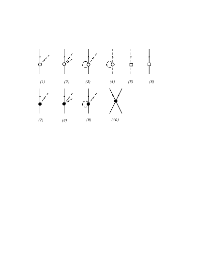
Figure 4: Vertices entering the PV potential at ${\rm N2LO}$. The solid (dash) lines represent nucleons (pions). The open (solid) symbols denote PC (PV) vertices. In diagrams (3) and (4) the vertices are tadpole contributions from the $3\pi NN$ and $4\pi$ interaction Hamiltonians, respectively. The open square on a pion line as in diagram (5) represents a $\pi\pi$ vertex coming from the $\ell_{3}$ and $\ell_{4}$ terms in ${\cal L}_{\pi\pi}^{(4)}$ and the $\delta m_{\pi}^{2}$ term. The open square on a nucleon line as in diagram (6) represents insertions from the $c_{1}$ term in ${\cal L}_{\pi N}^{(2)}$ and the $\delta M$ term.

The interaction vertices needed for the construction of the PV potential are summarized in Fig. 4. Note that in the power counting of these vertices below, we do not include the $1/\sqrt{\omega_{k}}$ normalization factors in the pion fields. We obtain:

1. $\pi NN$ vertices: The LO PC interaction term (of order $Q$) is

   $$H_{I}^{\pi NN}=\int{\rm d}^{3}x\;{g_{A}\over 2f_{\pi}}\overline{\psi}\gamma^{\mu}\gamma^{5}\vec{\tau}\cdot\partial_{\mu}\vec{\pi}\psi\ .$$ (211)

   giving the following vertex functions, see Eqs. (187) and (188),

   $${}^{PC}M^{01}_{\alpha^{\prime}\alpha,{\bm{q}}\,a} = -i{g_{A}\over 2f_{\pi}}{\xi_{t^{\prime}}^{\dagger}\tau_{a}\xi_{t}\over\sqrt{2\omega_{k}}}{\overline{u}_{\alpha^{\prime}}\over\sqrt{2E^{\prime}}}\,q\!\!\!/\,\gamma^{5}{u_{\alpha}\over\sqrt{2E}}\ ,$$ (212)

   $${}^{PC}M^{10}_{\alpha^{\prime}\alpha,{\bm{q}}\,a} = +i{g_{A}\over 2f_{\pi}}{\xi_{t^{\prime}}^{\dagger}\tau_{a}\xi_{t}\over\sqrt{2\omega_{k}}}{\overline{u}_{\alpha^{\prime}}\over\sqrt{2E^{\prime}}}\,q\!\!\!/\,\gamma^{5}{u_{\alpha}\over\sqrt{2E}}\ ,$$ (213)

   where $u_{\alpha}\equiv u({\bm{p}},s)$, etc., and $\xi_{t}$, $\xi_{t^{\prime}}$ are isospin states. The non-relativistic (NR) expansion of these amplitudes is needed up to order $Q^{2}$. Other PC $\pi NN$ vertices follow from the interactions terms in ${\cal L}_{N\pi}^{(3)}$ proportional to the LEC’s $d_{16}$ and $d_{18}$. Thus we find up to order $Q^{3}$ (spin-isospin states are suppressed for brevity):

   $${}^{PC}M^{\pi NN,01}_{\alpha^{\prime}\alpha,{\bm{q}}\,a} = {g_{A}\over 2f_{\pi}}{\tau_{a}\over\sqrt{2\omega_{q}}}\Bigl{[}i\,{\bm{q}}\cdot{\bm{\sigma}}-{i\over M}\omega_{q}\;{\bm{K}}\cdot{\bm{\sigma}}$$ (214)

   $$+ {i\over 4M^{2}}\Bigl{(}2{\bm{K}}\cdot{\bm{q}}\;{\bm{K}}\cdot{\bm{\sigma}}-2K^{2}\;{\bm{q}}\cdot{\bm{\sigma}}$$

   $$\qquad-{1\over 2}{\bm{k}}\cdot{\bm{\sigma}}\;{\bm{q}}\cdot{\bm{k}}\Bigr{)}\Bigr{]}$$

   $$+ {m_{\pi}^{2}\over f_{\pi}}(2d_{16}-d_{18}){\tau_{a}\over\sqrt{2\omega_{q}}}\;i{\bm{q}}\cdot{\bm{\sigma}}\ ,$$

   $${}^{PC}M^{\pi NN,10}_{\alpha^{\prime}\alpha,{\bm{q}}\,a} = -{}^{PC}M^{\pi NN,01}_{\alpha^{\prime}\alpha,{\bm{q}}\,a}.$$ (215)

   In diagrams, these PC vertex functions are represented as open circles. The PV $\pi NN$ vertices are due to interaction terms proportional to the LEC’s $h^{1}_{\pi}$, $h^{0}_{V}$, $h^{1}_{V}$, $h^{2}_{V}$, $h^{1}_{2}$, $h^{1}_{3}$, and $h^{1}_{12}$, and read up to order $Q^{2}$

   $${}^{PV}M^{\pi NN,01}_{\alpha^{\prime}\alpha,{\bm{q}}\,a} = -{h^{1}_{\pi}\over\sqrt{2}}{\epsilon_{3ab}\tau_{b}\over\sqrt{2\omega_{q}}}\Bigl{[}1-{2K^{2}+i({\bm{k}}\times{\bm{K}})\cdot{\bm{\sigma}}\over 4M^{2}}\Bigr{]}$$ (216)

   $$-{i\over f_{\pi}}\Bigl{(}{h^{0}_{V}\over 2}\tau_{a}+h^{1}_{V}\,\delta_{a,3}+{2\over 3}\,h^{2}_{V}\,{\cal I}^{ab}\,\tau_{b}\Bigr{)}$$

   $$\times{1\over\sqrt{2\omega_{q}}}\Bigl{(}\omega_{q}-{{\bm{q}}\cdot{\bm{K}}\over M}\Bigr{)}+{8\over f_{\pi}^{2}}{\epsilon_{3ab}\tau_{b}\over\sqrt{2\omega_{q}}}$$

   $$\times\Bigl{[}(h^{1}_{2}-h^{1}_{3})\,m_{\pi}^{2}-2h^{1}_{12}\,\omega_{q}^{2}\Bigr{]}\ ,$$

   $${}^{PV}M^{\pi NN,10}_{\alpha^{\prime}\alpha,{\bm{q}}\,a} = -{h^{1}_{\pi}\over\sqrt{2}}{\epsilon_{3ab}\tau_{b}\over\sqrt{2\omega_{q}}}\Bigl{[}1-{2K^{2}+i({\bm{k}}\times{\bm{K}})\cdot{\bm{\sigma}}\over 4M^{2}}\Bigr{]}$$ (217)

   $$+{i\over f_{\pi}}\Bigl{(}{h^{0}_{V}\over 2}\tau_{a}+h^{1}_{V}\,\delta_{a,3}+{2\over 3}\,h^{2}_{V}\,{\cal I}^{ab}\,\tau_{b}\Bigr{)}$$

   $$\times{1\over\sqrt{2\omega_{q}}}\Bigl{(}\omega_{q}-{{\bm{q}}\cdot{\bm{K}}\over M}\Bigr{)}+{8\over f_{\pi}^{2}}{\epsilon_{3ab}\tau_{b}\over\sqrt{2\omega_{q}}}$$

   $$\times\Bigl{[}(h^{1}_{2}-h^{1}_{3})\,m_{\pi}^{2}-2h^{1}_{12}\,\omega_{k}^{2}\Bigr{]}\ .$$

2. $\pi\pi NN$ vertices: The PC interaction is due to the Weinberg-Tomozawa term

   $$H_{I}^{\pi\pi NN}=\int{\rm d}^{3}x\;{1\over 4f_{\pi}^{2}}\overline{\psi}\,\gamma^{\mu}\vec{\tau}\cdot(\vec{\pi}\times\partial_{\mu}\vec{\pi})\,\psi\ ,$$ (218)

   and in the following only the LO in the NR expansion is needed at the order we are interested in. The corresponding vertex functions read

   $${}^{PC}M^{\pi\pi NN,02}_{\alpha^{\prime}\alpha,{\bm{q}}^{\prime}a^{\prime}\,{\bm{q}}\,a} = {i\over 8f_{\pi}^{2}}\epsilon_{aa^{\prime}b}\tau_{b}{\omega_{q}-\omega_{q^{\prime}}\over\sqrt{2\omega_{q}}\sqrt{2\omega_{q^{\prime}}}}\ ,$$ (219)

   $${}^{PC}M^{\pi\pi NN,11}_{\alpha^{\prime}\alpha,{\bm{q}}^{\prime}a^{\prime}\,{\bm{q}}\,a} = {i\over 4f_{\pi}^{2}}\epsilon_{aa^{\prime}b}\tau_{b}{\omega_{q}+\omega_{q^{\prime}}\over\sqrt{2\omega_{q}}\sqrt{2\omega_{q^{\prime}}}}\ ,$$ (220)

   $${}^{PC}M^{\pi\pi NN,20}_{\alpha^{\prime}\alpha,{\bm{q}}^{\prime}a^{\prime}\,{\bm{q}}\,a} = {i\over 8f_{\pi}^{2}}\epsilon_{aa^{\prime}b}\tau_{b}{\omega_{q^{\prime}}-\omega_{q}\over\sqrt{2\omega_{q}}\sqrt{2\omega_{q^{\prime}}}}\ ,$$ (221)

   and tadpole contributions vanish because of the isospin factor $\epsilon_{aa^{\prime}b}$. The PV vertices follow from the interaction terms proportional to $h^{1}_{A}$ and $h^{2}_{A}$, and are given by

   $${}^{PV}M^{\pi\pi NN,02}_{\alpha^{\prime}\alpha,{\bm{q}}^{\prime}a^{\prime}\,{\bm{q}}\,a} = {i\over 2f_{\pi}^{2}}{1\over\sqrt{2\omega_{q}}\sqrt{2\omega_{q^{\prime}}}}\Bigl{[}-h^{1}_{A}\,\epsilon_{3aa^{\prime}}({\bm{q}}-{\bm{q}}^{\prime})\cdot{\bm{\sigma}}$$ (222)

   $$-{1\over 3}h^{2}_{A}\,\epsilon_{aa^{\prime}b}\,I^{b}\,\tau_{b}\,({\bm{q}}-{\bm{q}}^{\prime})\cdot{\bm{\sigma}}$$

   $$+{1\over 3}h^{2}_{A}\,\epsilon_{aa^{\prime}b}\,\tau_{b}\,(I^{a}\,{\bm{q}}-I^{a^{\prime}}\,{\bm{q}}^{\prime})\cdot{\bm{\sigma}}\Bigr{]}\ ,$$

   $${}^{PV}M^{\pi\pi NN,11}_{\alpha^{\prime}\alpha,{\bm{q}}^{\prime}a^{\prime}\,{\bm{q}}\,a} = {i\over f_{\pi}^{2}}{1\over\sqrt{2\omega_{q}}\sqrt{2\omega_{q^{\prime}}}}\Bigl{[}-h^{1}_{A}\,\epsilon_{3aa^{\prime}}({\bm{q}}+{\bm{q}}^{\prime})\cdot{\bm{\sigma}}$$ (223)

   $$-{1\over 3}h^{2}_{A}\,\epsilon_{aa^{\prime}b}\,I^{b}\,\tau_{b}\,({\bm{q}}+{\bm{q}}^{\prime})\cdot{\bm{\sigma}}$$

   $$+{1\over 3}h^{2}_{A}\,\epsilon_{aa^{\prime}b}\,\tau_{b}\,(I^{a}\,{\bm{q}}+I^{a^{\prime}}\,{\bm{q}}^{\prime})\cdot{\bm{\sigma}}\Bigr{]}\ ,$$

   $${}^{PV}M^{\pi\pi NN,20}_{\alpha^{\prime}\alpha,{\bm{q}}^{\prime}a^{\prime}\,{\bm{q}}\,a} = {i\over 2f_{\pi}^{2}}{1\over\sqrt{2\omega_{q}}\sqrt{2\omega_{q^{\prime}}}}\Bigl{[}-h^{1}_{A}\,\epsilon_{3aa^{\prime}}\ ({\bm{q}}^{\prime}-{\bm{q}})\cdot{\bm{\sigma}}$$ (224)

   $$-{1\over 3}h^{2}_{A}\,\epsilon_{aa^{\prime}b}\,I^{b}\tau_{b}\,({\bm{q}}^{\prime}-{\bm{q}})\cdot{\bm{\sigma}}$$

   $$+{1\over 3}h^{2}_{A}\,\epsilon_{aa^{\prime}b}\,\tau_{b}\,(I^{a^{\prime}}\,{\bm{q}}^{\prime}-I^{a}\,{\bm{q}})\cdot{\bm{\sigma}}\Bigr{]}\ ,$$

   where the factor $I^{a}$ has been defined as $I^{a}=(-1,-1,2)$.

3. $3\pi NN$ vertices: We need consider the $3\pi NN$ interactions deriving from the expansion of the $U$ matrix given in Eq. (1) in both the PC and PV LO Lagrangians. The corresponding Hamiltonians read

   $$H_{I}^{3\pi NN} = -{g_{A}\over 2}\int{\rm d}^{3}x\;\overline{\psi}\Bigl{[}{4\alpha-1\over 2f_{\pi}^{3}}\gamma^{\mu}\gamma^{5}(\vec{\tau}\cdot\vec{\pi})(\vec{\pi}\cdot\partial_{\mu}\vec{\pi})$$ (226)

   $$\qquad\quad+{\alpha\over f_{\pi}^{3}}\gamma^{\mu}\gamma^{5}\,\vec{\pi}^{2}\,(\vec{\tau}\cdot\partial_{\mu}\vec{\pi})\Bigr{]}\psi$$

   $$+{h^{1}_{\pi}\over\sqrt{2}}{\alpha\over f_{\pi}^{2}}\int{\rm d}^{3}x\;\overline{\psi}\,\pi^{2}\,(\vec{\pi}\times\vec{\tau})_{3}\psi\ .$$

   Here we are interested only in tadpole contributions associated with these interactions. We denote them as $T^{3\pi NN}_{I}=T^{3\pi NN,01}+T^{3\pi NN,10}$, where

   $$T^{3\pi NN,01} = {1\over\sqrt{\Omega}}\sum_{\alpha^{\prime}\alpha}\sum_{{\bm{q}}\,a}b^{{\dagger}}_{\alpha^{\prime}}b_{\alpha}a_{{\bm{q}}\,a}\;M^{3\pi NN,01}_{\alpha^{\prime}\alpha,{\bm{q}}\,a}\delta_{{\bm{q}}+{\bm{p}},{\bm{p}}^{\prime}}\ ,$$

   $$T^{3\pi NN,10} = {1\over\sqrt{\Omega}}\sum_{\alpha^{\prime}\alpha}\sum_{{\bm{q}}\,a}b^{{\dagger}}_{\alpha^{\prime}}b_{\alpha}a^{\dagger}_{{\bm{q}}\,a}\;M^{3\pi NN,10}_{\alpha^{\prime}\alpha,{\bm{q}}\,a}\delta_{{\bm{q}}+{\bm{p}}^{\prime},{\bm{p}}}\ .$$

   The PC part is given by

   $${}^{PC}M^{3\pi NN,01}_{\alpha^{\prime}\alpha,{\bm{q}}\,a} = -i\,{g_{A}\over 8f_{\pi}^{3}}(10\,\alpha-1){\tau_{a}\over\sqrt{2\omega_{q}}}\,{\bm{\sigma}}\cdot{\bm{q}}\,J_{01}\ ,$$

   $${}^{PC}M^{3\pi NN,10}_{\alpha^{\prime}\alpha,{\bm{q}}\,a} = i\,{g_{A}\over 8f_{\pi}^{3}}(10\,\alpha-1){\tau_{a}\over\sqrt{2\omega_{q}}}\,{\bm{\sigma}}\cdot{\bm{q}}\,J_{01}\ ,$$

   where the (infinite) constants $J_{mn}$ have been defined as

   $$J_{mn}={1\over\Omega}\sum_{\bm{k}}{k^{2m}\over\omega_{k}^{n}}\ .$$ (227)

   The PV part reads

   $${}^{PV}\!M^{3\pi NN,01}_{\alpha^{\prime}\alpha,{\bm{q}}\,a}={}^{PV}\!M^{3\pi NN,10}_{\alpha^{\prime}\alpha,{\bm{q}}\,a}={5\over 2}{h^{1}_{\pi}\over\sqrt{2}}{\alpha\over f_{\pi}^{2}}{\epsilon_{3ab}\tau_{b}\over\sqrt{2\omega_{q}}}J_{01}\ .$$ (228)

4. $4\pi$ vertices: The relevant interaction Hamiltonian follows from the PC Lagrangian ${\cal L}^{(2)}_{\pi\pi}$ (there is no a PV contribution in this case), and is given by

   $$H_{I}^{4\pi} = \int d^{3}x\;\Bigl{[}-{1-4\alpha\over 2f_{\pi}^{2}}(\vec{\pi}\cdot\partial_{\mu}\vec{\pi})(\vec{\pi}\cdot\partial^{\mu}\vec{\pi})$$ (229)

   $$+{\alpha\over f_{\pi}^{2}}\vec{\pi}^{2}(\partial^{\mu}\vec{\pi}\cdot\partial_{\mu}\vec{\pi})-{8\alpha-1\over 8f_{\pi}^{2}}m_{\pi}^{2}\vec{\pi}^{4}\Bigr{]}\ .$$

   The associated tadpole contributions read $T^{4\pi}_{I}=T^{4\pi,02}+T^{4\pi,11}+T^{4\pi,20}$ are:

   $$T^{4\pi,02} = \sum_{{\bm{q}}\,a}a_{{\bm{q}}\,a}a_{-{\bm{q}}\,a}\;M^{4\pi,02}_{{\bm{q}}}\ ,$$ (230)

   $$T^{4\pi,11} = \sum_{{\bm{q}}\,a}a_{{\bm{q}}\,a}^{\dagger}a_{{\bm{q}}\,a}\;M^{4\pi,11}_{{\bm{q}}}\ ,$$ (231)

   $$T^{4\pi,20} = \sum_{{\bm{q}}\,a}a_{{\bm{q}}\,a}^{\dagger}a_{-{\bm{q}}\,a}^{\dagger}\;M^{4\pi,20}_{{\bm{q}}}\ ,$$ (232)

   with

   $${}^{PC}M^{4\pi,02}_{{\bm{q}}} = {1-10\alpha\over 4f_{\pi}^{2}}\omega_{q}J_{01}+{16\alpha-3\over 4f_{\pi}^{2}}J_{00}$$ (233)

   $$+{m_{\pi}^{2}\over 16f_{\pi}^{2}}{1\over\omega_{q}}J_{01}\ ,$$

   $${}^{PC}M^{4\pi,11}_{{\bm{q}}} = {m_{\pi}^{2}\over 8f_{\pi}^{2}}{1\over\omega_{q}}J_{01}\ ,$$ (234)

   $${}^{PC}M^{4\pi,20}_{{\bm{q}}} = {1-10\alpha\over 4f_{\pi}^{2}}\omega_{q}J_{01}-{16\alpha-3\over 4f_{\pi}^{2}}J_{00}$$ (235)

   $$+{m_{\pi}^{2}\over 16f_{\pi}^{2}}{1\over\omega_{q}}J_{01}\ .$$

5. $\pi\pi$ contact interactions: These follow from the two terms in ${\cal L}^{(4)}_{\pi\pi}$ and the $\delta m_{\pi}^{2}$ counter-term, and are represented by an open square in diagram 5 of Fig. 4. They are given by $H^{\pi\pi}_{I}=H^{\pi\pi,02}+H^{\pi\pi,11}+H^{\pi\pi,20}$, where

   $$H^{\pi\pi,02} = \sum_{{\bm{q}}a}a_{{\bm{q}}\,a}a_{-{\bm{q}}\,a}\;M^{\pi\pi,02}_{{\bm{q}}}\ ,$$ (236)

   $$H^{\pi\pi,11} = \sum_{{\bm{q}}a}a_{{\bm{q}}\,a}^{\dagger}a_{{\bm{q}}\,a}\;M^{\pi\pi,11}_{{\bm{q}}}\ ,$$ (237)

   $$H^{\pi\pi,20} = \sum_{{\bm{q}}a}a_{{\bm{q}}\,a}^{\dagger}a_{-{\bm{q}}\,a}^{\dagger}\;M^{\pi\pi,20}_{{\bm{q}}}\ ,$$ (238)

   with

   $${}^{PC}M^{\pi\pi,02}_{{\bm{q}}} = \Bigl{[}\ell_{3}{m_{\pi}^{4}\over f_{\pi}^{2}}+{\delta m_{\pi}^{2}\over 2}\Bigr{]}{1\over 2\omega_{q}}+\ell_{4}{m_{\pi}^{2}\over f_{\pi}^{2}}\omega_{q}\ ,$$ (239)

   $${}^{PC}M^{\pi\pi,11}_{{\bm{q}}} = \Bigl{[}\ell_{3}{m_{\pi}^{4}\over f_{\pi}^{2}}+{\delta m_{\pi}^{2}\over 2}\Bigr{]}{1\over\omega_{q}}\ ,$$ (240)

   and ${}^{PC}M^{\pi\pi,20}_{{\bm{q}}}={}^{PC}M^{\pi\pi,02}_{{\bm{q}}}$.

6. $NN$ contact interactions: These follow from the $c_{1}$ term in ${\cal L}_{\pi N}^{(2)}$ and the $\delta M$ counter-term, and are represented by an open square on a nucleon line in diagram 6 of Fig. 4. They are given by

   $$H^{NN}=\sum_{\alpha}b^{\dagger}_{\alpha}b_{\alpha}M^{NN}_{\bm{p}}\ ,\qquad M^{NN}_{\bm{p}}=-4c_{1}m_{\pi}^{2}\ .$$ (241)

7. $4N$ contact interaction: The EFT Hamiltonian includes also the term given in Eq. (186) derived from a contact Lagrangian. We only need its PV part of order $Q$, arising from the five independent interaction terms discussed in Ref. Girlanda08 . At order $Q$, with a suitable choice of the LEC’s, the vertex function ${}^{PV}M^{00}$ can be written as

   $${}^{PV}M^{00}_{\alpha_{1}^{\prime}\alpha_{1}\alpha_{2}^{\prime}\alpha_{2}} = {1\over 2\Lambda_{\chi}^{2}f_{\pi}}\Bigl{[}C_{1}({\bm{\sigma}}_{1}\times{\bm{\sigma}}_{2})\cdot{\bm{k}}_{1}$$ (242)

   $$+ C_{2}\,\vec{\tau}_{1}\cdot\vec{\tau}_{2}\,({\bm{\sigma}}_{1}\times{\bm{\sigma}}_{2})\cdot{\bm{k}}_{1}\;$$

   $$+ C_{3}\,(\vec{\tau}_{1}\times\vec{\tau}_{2})_{z}\,({\bm{\sigma}}_{1}+{\bm{\sigma}}_{2})\cdot{\bm{k}}_{1}\;$$

   $$+ C_{4}\,(\tau_{1z}+\tau_{2z})\,({\bm{\sigma}}_{1}\times{\bm{\sigma}}_{2})\cdot{\bm{k}}_{1}\;$$

   $$+ C_{5}\,{\cal I}^{ab}\,\tau_{1a}\,\tau_{2b}\,({\bm{\sigma}}_{1}\times{\bm{\sigma}}_{2})\cdot{\bm{k}}_{1}\;\Bigr{]}\ ,$$

   where ${\bm{k}}_{1}={\bm{p}}_{1}^{\prime}-{\bm{p}}_{1}=-{\bm{p}}_{2}^{\prime}+{\bm{p}}_{2}$.

Appendix G The PV potential

In this Appendix we report on the derivation of the PV $NN$ potential. In Sec. G.1 we discuss the nucleon and pion propagators, and in Sec. G.2 provide explicit expressions for the contributions of various diagrams.

G.1 The nucleon and pion propagators

We begin by considering the propagation of an isolated nucleon. Diagrams contributing to the transition amplitude $\langle\alpha^{\prime}|T|\alpha\rangle=T\,\delta_{\alpha^{\prime}\,\alpha}$ are displayed in Fig. 5.

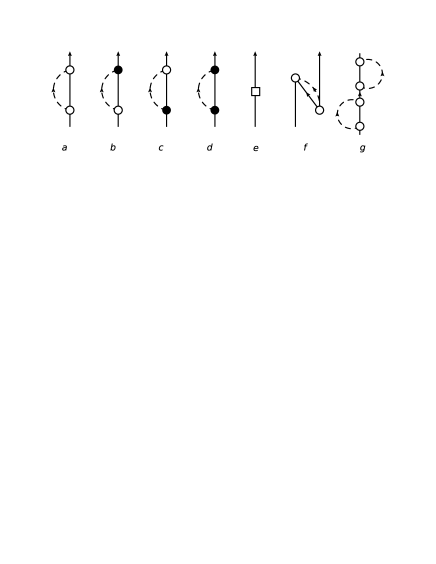
Figure 5: Diagrams describing the $N\rightarrow N$ transition amplitude. The open (solid) circles represent contributions due to PC (PV) $\pi NN$ vertices, while the open square represents the contribution from the $c_{1}$ term in ${\cal L}_{\pi N}^{(2)}$ and the $\delta M$ counterterm. The notation is as in Fig. 4.

Diagrams (a)-(d) are pion-loop contributions due to PC and PV $\pi NN$ vertices. The contribution of diagram (a) is of order $Q^{3}$, while those of diagrams (b) and (c) vanish, since the integrand is odd with respect to the loop momentum. The contribution of diagram (d) is ignored, since it contains two PV vertices. Diagram (e) represents the contribution from the two terms proportional to $\overline{\psi}\psi$ (namely, the $c_{1}$ term in ${\cal L}_{\pi N}^{(2)}$ of order $Q^{2}$ and the $\delta M$ counter-term), diagram (f) represents contributions associated with antinucleons, which enter first at order $Q^{4}$, and lastly diagram (g) is an example of a reducible two-loop contribution (of order $Q^{4}$). Contributions from reducible diagrams can be summed up analytically as shown below. Explicitly, the contribution of diagram (a) is

$$T({\rm a})={1\over\Omega}\sum_{\bm{k}}{3\,g^{2}_{A}\over 8\,f^{2}_{\pi}}\,{k^{2}\over\omega_{k}}{1\over E_{p}-E_{|{\bm{p}}-{\bm{k}}|}-\omega_{k}}\ ,$$ (243)

which to leading order $Q^{3}$ gives

$$T^{(3)}({\rm a})=-{1\over\Omega}\sum_{\bm{k}}{3\,g^{2}_{A}\over 8\,f^{2}_{\pi}}\,{k^{2}\over\omega_{k}^{2}}\ ,$$ (244)

while the contributions of diagrams (e) and (f) read, respectively,

$$T({\rm e}) = -4\,m^{2}_{\pi}\,c_{1}+\delta M\ ,$$ (245)

$$T^{(4)}({\rm f}) = {1\over\Omega}\sum_{\bm{k}}{3\,g^{2}_{A}\over 16\,f^{2}_{\pi}}\,{\omega_{k}\over M}\ ,$$ (246)

where only the leading order $Q^{4}$ has been retained in the case of diagram (f). We now set the $N\rightarrow N$ amplitude to zero order by order in the power counting by assuming

$$\delta M=\delta M^{(2)}+\delta M^{(3)}+\delta M^{(4)}+\cdots\ ,$$ (247)

where $\delta M^{(n)}$ is of order $Q^{n}$, and by determining $\delta M^{(n)}$ so that $T^{(n)}=0$. Up to order $Q^{4}$, we obtain

$$\delta M^{(2)} = 4\,m_{\pi}^{2}\,c_{1}\ ,\qquad\delta M^{(3)}=-T^{(3)}({\rm a})\ ,$$ (248)

$$\delta M^{(4)} = -T^{(4)}({\rm a})-T^{(4)}({\rm f})\ .$$ (249)

Figure 6: Parts of a general diagram with the propagation of nucleons only.

Next we consider the “dressing” of a nucleon line belonging to a more complicated diagram, see Fig. 6. Panel (a) on this figure represents a diagram in which one nucleon of momentum ${\bm{p}}$ is created at vertex 1 and annihilated at vertex 2 (shown by the two dots at the beginning and end of the nucleon line). The other nucleons have energies collectively denoted by $E_{r}$. Note that there are no pions in flight in the intermediate state. The energy denominator of the diagram in panel (a) is

$$P_{0}(E)={1\over E_{0}-(E_{p}+E_{r})+i\epsilon}={1\over E+i\epsilon}\ ,$$ (250)

where $E=E_{0}-E_{p}-E_{r}$ and $E_{0}$ is the initial energy (which depends on the particular process under consideration).

Panels (b) and (c) in Fig. 6 represent, respectively, the contribution in which nucleon 1 emits and reabsorbs a pion of momentum ${\bm{k}}$ and that in which a contact interaction occurs. These contributions are given by

$$S(E) = {1\over\Omega}\sum_{\bm{k}}{3\,g^{2}_{A}\over 8\,f^{2}_{\pi}}\,{k^{2}\over\omega_{k}}\,{1\over E+E_{p}-E_{|{\bm{p}}-{\bm{k}}|}-\omega_{k}}$$ (251)

$$-4\,m_{\pi}^{2}\,c_{1}+\delta M+\ldots\ ,$$

and $S(0)=0$ follows from the choice of $\delta M$ discussed previously for a single nucleon (of course, energy denominators in the diagrams of Figs. 5 and 6 are different, and $S(E)$ only vanishes for $E=0$).

By summing up repeated (b)- and (c)-type insertions, we obtain the well known result

$$P_{D}(E) = {1\over E+i\epsilon}+{1\over E+i\epsilon}S(E){1\over E+i\epsilon}+\cdots$$ (252)

$$= {1\over E-S(E)+i\epsilon}\ .$$

By expanding $S(E)$ in powers of $E$ ($E$ is assumed to be small) and by keeping only linear terms in $E$, we find

$$P_{D}(E) \simeq {1\over 1-S^{\prime}(0)}{1\over E+i\epsilon}={Z_{N}\over E+i\epsilon}\ ,$$ (253)

where $Z_{N}=1/[1-S^{\prime}(0)]$,

$$S^{\prime}(0)=-{1\over\Omega}\sum_{\bm{k}}{3\,g^{2}_{A}\over 8\,f^{2}_{\pi}}\,{k^{2}\over\omega_{k}^{3}}=-{3\,g^{2}_{A}\over 8\,f^{2}_{\pi}}\,J_{13}\ ,$$ (254)

and the (infinite) constant $J_{13}$ is defined in Eq. (97). Since $-E=E_{p}+E_{r}-E_{0}$ is the energy of the intermediate state relative to the initial energy, it is physically sensible that for $E\rightarrow 0$ the dressed operator should have the same form as the bare propagator $1/(E+i\epsilon)$ up to the (nucleon wave function) renormalization factor $Z_{N}$. In the following we adopt the common practice of attaching a $\sqrt{Z_{N}}$ at each of the two vertices of an internal nucleon line, and of multiplying by an extra $\sqrt{Z_{N}}$ each external nucleon line. The renormalization of nucleon lines when additional pions are present must be discussed case by case.

We now consider a diagram with an intermediate state involving a single pion of momentum ${\bm{k}}$ and energy $\omega_{k}$, and denote with $E_{0}$ the energy of the initial state and with $E_{r}$ the total energy of particles other than the pion present in this intermediate state. We assume that $|E_{0}-E_{r}|\ll\omega_{k}$. In Fig. 7, the various panels only show the (internal) pion line of this generic diagram.

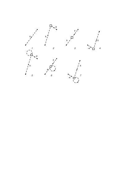
Figure 7: Propagation of a pion in the intermediate state of a generic diagram. Only the pion line is shown.

The energy denominator associated with a single pion propagation in panel (1) is $(E_{0}-\omega_{k}-E_{r}+i\epsilon)^{-1}\simeq-\omega_{k}^{-1}$. The two vertices at the beginning and end of the pion line each bring in a $(1/\sqrt{2\omega_{k}})$. Furthermore, there is factor $2$ coming from the two possible time orderings in the propagation of the pion (“left-to-right” and “right-to-left”). Thus the bare pion propagator is $-1/\omega_{k}^{2}$. By taking into account the remaining contributions from panels (2)-(7) in Fig. 7, we find the “dressed” propagator up to corrections of order $Q^{2}$ included to be given by

$$S_{\pi}({\bm{k}})\simeq-{1\over\omega_{k}^{2}}\left(1-{A_{\pi}\over\omega_{k}^{2}}+\delta Z_{\pi}\right)\ ,$$ (255)

where

$$A_{\pi} = {2\,\ell_{3}\,m^{4}_{\pi}\over f_{\pi}^{2}}+{m^{2}_{\pi}\over 4\,f_{\pi}^{2}}\,J_{01}+\delta m_{\pi}^{2}\ ,$$ (256)

$$\delta Z_{\pi} = -{2\,\ell_{4}\,m^{2}_{\pi}\over f_{\pi}^{2}}-{1-10\,\alpha\over 2\,f_{\pi}^{2}}\,J_{01}\ .$$ (257)

Note that $A_{\pi}/\omega_{k}^{2}$ and $\delta Z_{\pi}$ are both of order $Q^{2}$. The dressed propagator $S_{\pi}({\bm{k}})$ can also be written as

$$S_{\pi}({\bm{k}})\simeq-{1+\delta Z_{\pi}\over\omega_{k}^{2}+A_{\pi}}\ .$$ (258)

Here $Z_{\pi}=1+\delta Z_{\pi}$ represents the renormalization of the pion wave function, and again we attach a factor $\sqrt{Z_{\pi}}$ at each of the two ends of the pion line. Therefore this factor contributes to the renormalization of the coupling constants. The term $A_{\pi}$ represents the shift in the square of the pion mass, and in order to have $m^{2}_{\pi}$ be the physical pion mass, we choose $\delta m_{\pi}^{2}$ so that $A_{\pi}=0$. The expressions above for $A_{\pi}$ and $\delta Z_{\pi}$ are the same as those reported in Eq. (2.39) of Ref. Epel03 .

G.2 The PV $NN$ potential

Diagrams contributing to the PV $NN$ amplitude up to order $Q$ are shown in Figs. 1 and 2. The power counting is as follows: (i) a PC (PV) $\pi NN$ vertex is of order $Q$ ($Q^{0}$); (ii) a PC or PV $\pi\pi NN$ vertex is of order $Q^{1}$; (iii) a PC (PV) $NN$ contact vertex is of order $Q^{0}$ ($Q$); (iv) an energy denominator without (with one or more) pions is of order $Q^{-2}$ ($Q^{-1}$); (v) factors $Q^{-1}$ and $Q^{3}$ are associated with, respectively, each pion line and each loop integration. The momenta are defined as given below Eq. (91), and in what follows use is made of the fact that ${\bm{k}}\cdot{\bm{K}}$ vanishes in the CM frame.

The PV $NN$ potential is derived from the amplitudes in Figs. 1 and 2 via Eqs. (88)–(90). Up to order $Q$ included, we obtain for the OPE component in panel (a) of Fig. 1 :

$$V({\rm a})=V^{(-1)}({\rm NR})+V^{(1)}({\rm RC})+V^{(1)}({\rm LEC})\ ,$$ (259)

where

$$V^{(-1)}({\rm NR})\!\! = \!\!{g_{A}h^{1}_{\pi}\over 2\sqrt{2}f_{\pi}}(\vec{\tau}_{1}\times\vec{\tau}_{2})_{z}{i{\bm{k}}\cdot({\bm{\sigma}}_{1}\!+\!{\bm{\sigma}}_{2})\over\omega_{k}^{2}}\ ,$$ (260)

$$V^{(1)}({\rm RC})\!\! = \!\!{g_{A}h^{1}_{\pi}\over 2\sqrt{2}f_{\pi}}\,{1\over 4M^{2}}\,(\vec{\tau}_{1}\times\vec{\tau}_{2})_{z}\;{1\over\omega_{k}^{2}}$$ (261)

$$\times\biggl{[} -\frac{i}{2}\left(8K^{2}+k^{2}\right)\,{\bm{k}}\cdot({\bm{\sigma}}_{1}+{\bm{\sigma}}_{2})$$

$$+ \!{\bm{k}}\cdot{\bm{\sigma}}_{1}\,\,({\bm{k}}\times{\bm{K}})\!\cdot\!{\bm{\sigma}}_{2}$$

$$+ \!{\bm{k}}\!\cdot\!{\bm{\sigma}}_{2}\,\,({\bm{k}}\times{\bm{K}})\cdot{\bm{\sigma}}_{1}\biggr{]}\ ,\qquad\quad$$

$$V^{(1)}({\rm LEC}) = V^{(-1)}({\rm NR})\biggl{[}{2\,m_{\pi}^{2}\over g_{A}}\,(2\,d_{16}-d_{18})$$ (262)

$$\qquad-{8\sqrt{2}\,m^{2}_{\pi}\over h^{1}_{\pi}\,f_{\pi}^{2}}(h^{1}_{2}-h^{1}_{3})\biggr{]}$$

$$+ {16\,h^{1}_{12}\over f_{\pi}^{2}}{g_{A}\over 2\,f_{\pi}}(\vec{\tau}_{1}\times\vec{\tau}_{2})_{z}\;i{\bm{k}}\cdot({\bm{\sigma}}_{1}\!+\!{\bm{\sigma}}_{2})\ .\qquad$$

The potential does not depend on the LEC’s $h^{0}_{V}$, $h^{1}_{V}$, and $h^{2}_{V}$, since the associated contributions cancel out when summing over the different time orderings. The factor $k^{2}=\omega_{k}^{2}-m_{\pi}^{2}$ in $V^{(1)}({\rm RC})$ leads to a piece that can be reabsorbed in the contact term proportional to $C_{3}$ in Eq. (109) and a piece proportional to $m_{\pi}^{2}$ that simply renormalizes the LEC $h^{1}_{\pi}$. Similarly, the piece in $V^{(1)}({\rm LEC})$ proportional to $V^{(-1)}({\rm NR})$ leads to renormalization of $h_{\pi}^{1}$ and the remaining term can be reabsorbed in $C_{3}$. We are then left with the components $V_{PV}^{\rm(OPE)}$ and $V_{PV}^{\rm(RC)}$ given in Eqs. (98) and (108).

The component of the PV potential due to the contact terms in panel CT of Fig. 1 derives directly from the vertex function ${}^{PV}M^{00}$ given in Eq. (242). The final expression has already been given in Eq. (109).

The panels (b) and (c) contain a combination of a contact interaction with the exchange of a pion. However, it can be shown that their contribution is at least of order $Q^{3}$.

Next we consider the TPE components in panels (d)-(g). The contribution from panel (d) reads

$$V^{(1)}({\rm d}) = {g_{A}h^{1}_{\pi}\over 8\sqrt{2}f_{\pi}^{3}}\,(\vec{\tau}_{1}\times\vec{\tau}_{2})_{z}\,i\,{\bm{k}}\cdot({\bm{\sigma}}_{1}+{\bm{\sigma}}_{2})$$ (263)

$$\int{{\rm d}^{3}q\over(2\pi)^{3}}\;{1\over\omega_{+}\omega_{-}(\omega_{+}+\omega_{-})}\ ,$$

where $\omega_{\pm}=\sqrt{({\bm{k}}\pm{\bm{q}})^{2}+4\,m_{\pi}^{2}}$. Use of dimensional regularization allows one to obtain the finite part as Pastore09

$$\overline{V}^{(1)}({\rm d})=-{g_{A}h^{1}_{\pi}\over 2\sqrt{2}f_{\pi}\Lambda_{\chi}^{2}}(\vec{\tau}_{1}\times\vec{\tau}_{2})_{z}\,i{\bm{k}}\cdot({\bm{\sigma}}_{1}+{\bm{\sigma}}_{2})\;L(k)\ ,$$ (264)

where $\Lambda_{\chi}=4\pi f_{\pi}$ and the loop function $L(k)$ is defined as

$$L(k)={1\over 2}{s\over k}\ln\left({s+k\over s-k}\right)\ ,\quad s=\sqrt{k^{2}+4\,m^{2}_{\pi}}\ .$$ (265)

The singular part is given by

$$V^{(1)}_{\infty}({\rm d})=-{g_{A}h^{1}_{\pi}\over 4\sqrt{2}f_{\pi}\Lambda_{\chi}^{2}}(\vec{\tau}_{1}\times\vec{\tau}_{2})_{z}i{\bm{k}}\cdot({\bm{\sigma}}_{1}+{\bm{\sigma}}_{2})\;(d^{\prime}_{\epsilon}-2)\ ,$$ (266)

where

$$d^{\prime}_{\epsilon}=-{2\over\epsilon}+\gamma-\ln\pi+\ln\left({m^{2}_{\pi}\over\mu^{2}}\right)\ ,$$ (267)

$\epsilon=3-d$, $d$ being the number of dimensions ($d\rightarrow 3$), and $\mu$ is a renormalization scale. This singular contribution is absorbed in the $V^{({\rm CT})}$ term proportional to $C_{3}$.

The contributions from panels (e), (f), and (g) in Fig. 1 are collectively denoted as “box” below, and the non-iterative pieces in reducible diagrams of type (g) are identified via Eq. (90)—elsewhere Pastore09 , they have been referred to as the “recoil corrections”. We obtain

$$V^{(1)}({\rm box})\! = \!\!{g_{A}h^{1}_{\pi}\over 2\sqrt{2}f_{\pi}}{g_{A}^{2}\over 4f_{\pi}^{2}}\int{{\rm d}^{3}q\over(2\pi)^{3}}\;{\omega_{+}^{2}+\omega_{+}\omega_{-}+\omega_{-}^{2}\over\omega_{+}^{3}\omega_{-}^{3}(\omega_{+}+\omega_{-})}\biggl{[}-2i\,(\tau_{1z}+\tau_{2z})\;\Bigl{[}{\bm{q}}\cdot{\bm{\sigma}}_{1}\,({\bm{q}}\times{\bm{k}})\cdot{\bm{\sigma}}_{2}$$ (268)

$$\!\!-{\bm{q}}\cdot{\bm{\sigma}}_{2}\,({\bm{q}}\times{\bm{k}})\cdot{\bm{\sigma}}_{1}\Bigr{]}\!-\!2i\,(\tau_{1z}-\tau_{2z})\,\Bigl{[}{\bm{q}}\cdot{\bm{\sigma}}_{1}\,\,({\bm{q}}\times{\bm{k}})\cdot{\bm{\sigma}}_{2}+{\bm{q}}\cdot{\bm{\sigma}}_{2}\,\,({\bm{q}}\times{\bm{k}})\cdot{\bm{\sigma}}_{1}\Bigr{]}$$

$$+i\,(\vec{\tau}_{1}\times\vec{\tau}_{2})_{z}\,(k^{2}-q^{2})\,\,{\bm{k}}\cdot({\bm{\sigma}}_{1}+{\bm{\sigma}}_{2})\biggr{]}\ ,$$

and, after dimensional regularization, the finite part reads

$$\overline{V}^{(1)}({\rm box})=\qquad\qquad\qquad\qquad$$ (269)

$$-{g_{A}^{3}\,h^{1}_{\pi}\over 2\sqrt{2}f_{\pi}\Lambda_{\chi}^{2}}\Bigl{[}4(\tau_{1z}+\tau_{2z})\;i{\bm{k}}\cdot({\bm{\sigma}}_{1}\times{\bm{\sigma}}_{2})L(k)$$

$$+(\vec{\tau}_{1}\times\vec{\tau}_{2})_{z}\,i{\bm{k}}\!\cdot\!({\bm{\sigma}}_{1}+{\bm{\sigma}}_{2})\bigl{[}H(k)-3\,L(k)\bigr{]}\Bigr{]}\ ,$$

where

$$H(k)={4\,m^{2}_{\pi}\over s^{2}}L(k)\ ,$$ (270)

while the singular part is given by

$$\overline{V}^{(1)}({\rm box})=\qquad\qquad\qquad$$ (271)

$$-{g_{A}^{3}\,h^{1}_{\pi}\over 2\sqrt{2}f_{\pi}\Lambda_{\chi}^{2}}\biggl{[}2\,(\tau_{1z}+\tau_{2z})\;i{\bm{k}}\cdot({\bm{\sigma}}_{1}\times{\bm{\sigma}}_{2})\;\Bigl{(}d^{\prime}_{\epsilon}-{4\over 3}\Bigr{)}$$

$$-(\vec{\tau}_{1}\times\vec{\tau}_{2})_{z}\,i{\bm{k}}\cdot({\bm{\sigma}}_{1}+{\bm{\sigma}}_{2})\;\Bigl{(}{3\over 2}d^{\prime}_{\epsilon}-1\Bigr{)}\biggr{]}\ .$$

The latter is absorbed in the $V^{({\rm CT})}$ terms proportional to $C_{3}$ and $C_{4}$.

We now turn our attention to the contributions from panels (h)-(u) in Fig. 2. Those from panels (h) and (i) represent the renormalization of nucleon external lines, discussed in subsection G.1, and cancel out due the choice of the mass counter-term $\delta M$. However, there is a factor of $\sqrt{Z_{N}}$ which needs to be included for each of the nucleon external lines. A correction of order $Q$ to the PV OPE potential follows given by

$$V^{(1)}({\rm h}\!+\!{\rm i}) = \Bigl{[}\Bigl{(}\sqrt{Z_{N}}\Bigl{)}^{4}-1\Bigl{]}\,\,V^{(-1)}({\rm NR})$$ (272)

$$= -{3\,g^{2}_{A}\over 4\,f^{2}_{\pi}}\,J_{13}\,\,V^{(-1)}({\rm NR})\ .$$

The contributions from panels (j), (k), and (l), which are of order $Q$, cancel out; in particular, diagrams of the (j)- and (k)-type, but where the PV $\pi NN$ vertex occurs in the pion loop, vanish (the integrand in the loop integration is odd). The contributions from panels (m) and (n) represent vertex corrections of order $Q$, given by

$$V^{(1)}({\rm m}\!+\!{\rm n})={g^{2}_{A}\over 12\,f^{2}_{\pi}}\,J_{13}\,\,V^{(-1)}({\rm NR})\ .$$ (273)

Note that hereafter we ignore factors of $\sqrt{Z_{N}}$, since they would lead to corrections of order higher than $Q$. The contributions from panels (o) and (p) are tadpoles originating from the interaction Hamiltonian $H^{3\pi NN}$,

$$V^{(1)}({\rm o}\!+\!{\rm p})=-{20\,\alpha-1\over 4f_{\pi}^{2}}\,J_{01}\,\,V^{(-1)}({\rm NR})\ .$$ (274)

The contributions from panels (q) and (r) represent renormalizations of the (internal) pion line (see Sec. G.1),

$$V^{(1)}({\rm q}\!+\!{\rm r})=\left(-{A_{\pi}\over\omega_{k}^{2}}+\delta Z_{\pi}\right)\,\,V^{(-1)}({\rm NR})\ ,$$ (275)

where $A_{\pi}$ and $\delta Z_{\pi}$ are the quantities defined in Eqs. (256) and (257); in particular, $A_{\pi}=0$ because of our choice to work with the physical pion mass, and $\delta Z_{\pi}$ contributes to the renormalization of the PC $\pi NN$ vertex. Finally, the contributions from panels (s), (t), and (u) represent vertex corrections. Those involving the PC $\pi\pi NN$ vertex read

$$V^{(1)}({\rm s}\!+\!{\rm t}\!+\!{\rm u})={1\over 4\,f_{\pi}^{2}}\,J_{01}\,\,V^{(-1)}({\rm NR})\ ,$$ (276)

However, contributions from diagrams involving the PV $\pi\pi NN$ vertex are at least of order $Q^{2}$.

We conclude by noting that an analysis of $\pi NN$ vertex corrections was also carried out in Ref. Zhu01 (in that paper the choice $\alpha=1/6$ in Eq. (1) was adopted). Our expressions are in agreement with those reported there.

Appendix H The potential in configuration space

In this Appendix, all the LEC’s are considered to be the renormalized ones (with the overlines omitted for simplicity). The configuration space expressions follow from Eq. (110) and read

$$V_{PV}({\bm{r}},{\bm{p}})=V^{({\rm OPE})}({\bm{r}})+V^{({\rm TPE})}({\bm{r}})+V^{({\rm RC})}({\bm{r}},{\bm{p}})+V^{({\rm CT})}({\bm{r}})\ ,$$ (277)

where ${\bm{p}}=-i{\bm{\nabla}}$ is the relative momentum operator and

$$V^{({\rm OPE})}({\bm{r}}) = {g_{A}h^{1}_{\pi}\over 2\sqrt{2}f_{\pi}}\,(\vec{\tau}_{1}\times\vec{\tau}_{2})_{z}\;({\bm{\sigma}}_{1}+{\bm{\sigma}}_{2})\cdot\hat{\bm{r}}\,g^{\prime}(r)\ ,$$ (278)

$$V^{({\rm TPE})}({\bm{r}}) = -{g_{A}h^{1}_{\pi}\over 2\sqrt{2}f_{\pi}}{m_{\pi}^{2}\over\Lambda_{\chi}^{2}}(\vec{\tau}_{1}\times\vec{\tau}_{2})_{z}({\bm{\sigma}}_{1}+{\bm{\sigma}}_{2})\cdot\hat{\bm{r}}\,L^{\prime}(r)$$ (279)

$$-{g_{A}h^{1}_{\pi}\over 2\sqrt{2}f_{\pi}}{g_{A}^{2}m_{\pi}^{2}\over\Lambda_{\chi}^{2}}\biggl{[}4\,(\tau_{1z}+\tau_{2z})\;({\bm{\sigma}}_{1}\times{\bm{\sigma}}_{2})\cdot\hat{\bm{r}}\,L^{\prime}(r)\;$$

$$+(\vec{\tau}_{1}\times\vec{\tau}_{2})_{z}({\bm{\sigma}}_{1}+{\bm{\sigma}}_{2})\cdot\hat{\bm{r}}\Bigl{[}H^{\prime}(r)-3L^{\prime}(r)\Bigr{]}\biggr{]}\ ,$$

$$V^{({\rm RC})}({\bm{r}},{\bm{p}}) = -{g_{A}h^{1}_{\pi}\over 2\sqrt{2}f_{\pi}4M^{2}}(\vec{\tau}_{1}\times\vec{\tau}_{2})_{z}$$ (280)

$$\biggl{[}\bigl{\{}p_{j}\,,\,\bigl{\{}p_{j}\,,\,({\bm{\sigma}}_{1}+{\bm{\sigma}}_{2})\cdot\hat{\bm{r}}\,g^{\prime}(r)\bigr{\}}\bigr{\}}$$

$$+ {\epsilon_{j\ell m}\over 2}\Bigl{(}\sigma_{1i}\,\sigma_{2j}+\sigma_{1j}\,\sigma_{2i}\Bigr{)}\,\Bigl{\{}p_{m}\,,\,\partial_{i}\,\partial_{\ell}g(r)\Bigr{\}}\biggr{]}\ ,$$

$$V^{({\rm CT})}({\bm{r}}) = {m_{\pi}^{2}\over\Lambda_{\chi}^{2}f_{\pi}}\Bigl{[}C_{1}({\bm{\sigma}}_{1}\times{\bm{\sigma}}_{2})\cdot\hat{\bm{r}}$$ (281)

$$\quad+C_{2}\,\vec{\tau}_{1}\cdot\vec{\tau}_{2}\,({\bm{\sigma}}_{1}\times{\bm{\sigma}}_{2})\cdot\hat{\bm{r}}\;$$

$$\quad+C_{3}\,(\vec{\tau}_{1}\times\vec{\tau}_{2})_{z}\,({\bm{\sigma}}_{1}+{\bm{\sigma}}_{2})\cdot\hat{\bm{r}}\;$$

$$\quad+C_{4}\,(\tau_{1z}+\tau_{2z})\,({\bm{\sigma}}_{1}\times{\bm{\sigma}}_{2})\cdot\hat{\bm{r}}\;$$

$$\quad+C_{5}\,{\cal I}^{ab}\,\tau_{1a}\,\tau_{2b}\,({\bm{\sigma}}_{1}\times{\bm{\sigma}}_{2})\cdot\hat{\bm{r}}\;\Bigr{]}Z^{\prime}(r)\ ,$$

with

$$g(r) = \int{{\rm d}^{3}k\over(2\pi)^{3}}\;{C_{\Lambda}(k)\over k^{2}+m_{\pi}^{2}}\,e^{i{\bm{k}}\cdot{\bm{r}}}\ ,$$ (282)

$$L(r) = \int{{\rm d}^{3}k\over(2\pi)^{3}}\;{C_{\Lambda}(k)\over m_{\pi}^{2}}L(k)\,e^{i{\bm{k}}\cdot{\bm{r}}}\ ,$$ (283)

$$H(r) = \int{{\rm d}^{3}k\over(2\pi)^{3}}\;{C_{\Lambda}(k)\over m_{\pi}^{2}}H(k)\,e^{i{\bm{k}}\cdot{\bm{r}}}\ ,$$ (284)

$$Z(r) = \int{{\rm d}^{3}k\over(2\pi)^{3}}\;{C_{\Lambda}(k)\over m_{\pi}^{2}}\,e^{i{\bm{k}}\cdot{\bm{r}}}\ .$$ (285)

Note that

$$\bigl{\{}p_{j}\,,\,\bigl{\{}p_{j}\,,\,O\bigr{\}}\bigr{\}} = -\left({\bm{\nabla}}^{2}O\right)$$ (286)

$$-4\,\left[\left({\bm{\nabla}}O\right)\cdot{\bm{\nabla}}+4\,O{\bm{\nabla}}^{2}\right]\ ,$$

and

$${\bm{\nabla}}^{2}({\bm{\sigma}}_{1}+{\bm{\sigma}}_{2})\cdot\hat{\bm{r}}\,g^{\prime}(r)\qquad\qquad\qquad\$$ (287)

$$= ({\bm{\sigma}}_{1}+{\bm{\sigma}}_{2})\cdot\hat{\bm{r}}\,\Bigl{[}g^{\prime\prime\prime}(r)+2\,{g^{\prime\prime}(r)\over r}-2\,{g^{\prime}(r)\over r^{2}}\Bigr{]}\ ,$$

$$\partial_{j}({\bm{\sigma}}_{1}+{\bm{\sigma}}_{2})\cdot\hat{\bm{r}}\,g^{\prime}(r)=(\sigma_{1j}+\sigma_{2j})\,{g^{\prime}(r)\over r}\qquad\qquad\qquad\$$ (288)

$$+({\bm{\sigma}}_{1}+{\bm{\sigma}}_{2})\cdot\hat{\bm{r}}\,\Bigl{[}{g^{\prime\prime}(r)\over r}-{g^{\prime}(r)\over r^{2}}\Bigr{]}\,{r_{j}\over r}\ ,$$

It is convenient to define the operators

$$S_{r}^{\pm} = ({\bm{\sigma}}_{1}\pm{\bm{\sigma}}_{2})\cdot\hat{\bm{r}}\ ,$$ (289)

$$S_{p}^{\pm} = ({\bm{\sigma}}_{1}\pm{\bm{\sigma}}_{2})\cdot{\bm{p}}\ ,$$ (290)

$$S_{r}^{\times} = ({\bm{\sigma}}_{1}\times{\bm{\sigma}}_{2})\cdot\hat{\bm{r}}\ ,$$ (291)

$$S_{L} = {\bm{\sigma}}_{1}\cdot\hat{\bm{r}}\,\,{\bm{\sigma}}_{2}\cdot\hat{{\bm{L}}}+{\bm{\sigma}}_{2}\cdot\hat{\bm{r}}\,\,{\bm{\sigma}}_{1}\cdot\hat{\bm{L}}\ ,$$ (292)

where $\hat{\bm{L}}=\hat{\bm{r}}\times{\bm{p}}$ is the “reduced” orbital angular momentum operator. In terms of these, $V^{({\rm RC})}({\bm{r}},{\bm{p}})$ can be written as

$$V^{({\rm RC})}({\bm{r}},{\bm{p}})={g_{A}h^{1}_{\pi}\over 4\sqrt{2}F_{\pi}M^{2}}(\vec{\tau}_{1}\times\vec{\tau}_{2})_{z}\qquad\qquad\qquad$$ (293)

$$\Biggl{[}\Bigl{[}g^{\prime\prime\prime}(r)+2{g^{\prime\prime}(r)\over r}-2{g^{\prime}(r)\over r^{2}}\Bigr{]}S^{+}_{r}$$

$$\ \ +4\,i\biggl{[}{g^{\prime}(r)\over r}\,S^{+}_{p}+\Bigl{[}g^{\prime\prime}(r)-{g^{\prime}(r)\over r}\Bigr{]}\,S_{r}^{+}\,\hat{\bm{r}}\cdot{\bm{p}}\biggr{]}$$

$$\ \ -4\,g^{\prime}(r)\;S^{+}_{r}\;{\bm{p}}^{2}\;-\Bigl{[}g^{\prime\prime}(r)-{g^{\prime}(r)\over r}\Bigr{]}\,S_{L}\Biggr{]}\ .$$

The functions $g(r)$, $L(r)$, $H(r)$, and $Z(r)$ are calculated numerically by standard quadrature techniques. It is easily seen that $g^{\prime\prime}(r)-g^{\prime}(r)/r$ and $g^{\prime\prime\prime}(r)+2\,g^{\prime\prime}(r)/r-2\,g^{\prime}(r)/r^{2}$ are well-behaved as $r\rightarrow 0$.

References

- (1) M.J. Ramsey-Musolf and S.A. Page, Ann. Rev. Nucl. Part. Sci. 56, 1 (2006) (arXiv:0601127 [hep-ph]).
- (2) W.C. Haxton and B.R. Holstein, Prog. Part. Nucl. Phys., 71, 185 (2013) (arXiv:1303.4132 [nucl-th]).
- (3) M.R. Schindler and R.P. Springer, Prog. Part. Nucl. Phys., 72, 1 (2013) (arXiv:1305.4190 [nucl-th]).
- (4) B. Desplanques, J.F. Donoghue, and B.R. Holstein, Ann. Phys. (N.Y.) 124, 449 (1980).
- (5) S. Weinberg, Phys. Lett. B 251, 288 (1990); Nucl. Phys. B 363, 3 (1991); Phys. Lett. B 295, 114 (1992).
- (6) C. Ordonez, L. Ray, and U. van Kolck, Phys. Rev. C 53, 2086 (1996).
- (7) E. Epelbaum, H.W. Hammer, and U.-G. Meissner, Rev. Mod. Phys. 81, 1773 (2009).
- (8) R. Machleidt and D.R. Entem, Phys. Rep. 503, 1 (2011).
- (9) S. Weinberg, Phys. Rev. Lett. 17, 616 (1966); Phys. Rev. 166, 1568 (1968); Physica A 96, 327 (1979).
- (10) C. Callan, S. Coleman, J. Wess, and B. Zumino, Phys. Rev. 177, 2247 (1969).
- (11) V. Bernard, N. Kaiser, and U.-G. Meissner, Int. J. Mod. Phys. E 4, 193 (1995).
- (12) T.-S. Park, D.-P. Min, and M. Rho, Nucl. Phys. A 596, 515 (1996); Y.-H. Song, R. Lazauskas, and T.-S. Park, Phys. Rev. C 79, 064002 (2009).
- (13) T.-S. Park et al., Phys. Rev. C 67, 055206 (2003).
- (14) S. Kölling, E. Epelbaum, H. Krebs, and U.-G. Meissner, Phys. Rev. C 80, 045502 (2009).
- (15) S. Pastore, L. Girlanda, R. Schiavilla, M. Viviani, and R.B. Wiringa Phys. Rev. C 80, 034004 (2009).
- (16) S. Kölling, E. Epelbaum, H. Krebs, and U.-G. Meissner, Phys. Rev. C 84, 054008 (2011).
- (17) S. Pastore, L. Girlanda, R. Schiavilla, and M. Viviani, Phys. Rev. C 84, 024001 (2011).
- (18) M. Piarulli et al., Phys. Rev. C 87, 014006 (2013).
- (19) J. Carlson and R. Schiavilla, Rev. Mod. Phys. 70, 743 (1998).
- (20) D.B. Kaplan and M.J. Savage, Nucl. Phys. A 556, 653 (1993); Erratum ibid. A 570, 833 (1994); Erratum ibid. A 580, 679 (1994).
- (21) J. Wasem, Phys. Rev. C 85, 022501 (2012).
- (22) S.L. Zhu, C.M. Maekawa, B.R. Holstein, M.J. Ramsey-Musolf, and U. van Kolck, Nucl. Phys. A 748, 435 (2005).
- (23) S.L. Zhu, S.J. Puglia, B.R. Holstein, and M.J. Ramsey-Musolf, Phys. Rev. D 62, 033008 (2000).
- (24) S.L. Zhu, S.J. Puglia, B.R. Holstein, and M.J. Ramsey-Musolf, Phys. Rev. D 63, 033006 (2001).
- (25) L. Girlanda, Phys. Rev. C 77, 067001 (2008).
- (26) G.S. Danilov, Phys. Lett. 18, 40 (1965).
- (27) J. de Vries, U.-G. Meissner, E. Epelbaum, and N. Kaiser, arXiv:1309.4711 [nucl-th].
- (28) B. Desplanques, C.H. Hyun, S. Ando, and C.-P. Liu, Phys. Rev. C 77, 064002 (2008).
- (29) C.-P. Liu, Phys. Rev. C 75, 065501 (2007).
- (30) C.H. Hyun, S. Ando, and B. Desplanques, Phys. Lett. B 651, 257 (2007).
- (31) C.H. Hyun, B. Desplanques, S. Ando, and C.-P. Liu, Mod. Phys. Lett. A 23, 2293 (2008).
- (32) J. de Vries, E. Mereghetti, R.G.E. Timmermans, and U. van Kolck, Annals Phys. 338, 50 (2013).
- (33) R. Balzer et al., Phys. Rev. Lett. 44, 699 (1980).
- (34) V. Yuan et al., Phys. Rev. Lett. 57, 1680 (1986).
- (35) P.D. Eversheim et al., Phys. Lett. B 256, 11 (1991).
- (36) S. Kistryn et al., Phys. Rev. Lett. 58, 1616 (1987).
- (37) A.R. Berdoz et al., Phys. Rev. C 68, 034004 (2003).
- (38) J. Lang et al., Phys. Rev. Lett. 54, 170 (1985).
- (39) J.F. Cavaignac, B. Vignon, and R. Wilson, Phys. Lett. B 67, 148 (1977).
- (40) M.T. Gericke et al., Nucl. Inst. Meth. A 611, 239 (2009).
- (41) V.A. Knyaz’kov et al., Nucl. Phys. A 417, 209 (1994).
- (42) W.M. Snow, Nucl. Inst. Meth. A 611, 248 (2009).
- (43) C.D. Bass et al., Nucl. Inst. Meth. A 612, 69 (2009).
- (44) D.M. Markoff, private communication.
- (45) J.D. Bowman (PI), C.B. Crawford (PI), M.T. Gericke (PI) et al., A Measurement of the Parity Violating Proton Asymmetry in the Capture of Polarized Cold Neutrons on 3He, proposal submitted to the SNS FNPB PRAC T, 2007-11-25.
- (46) R. Schiavilla, J. Carlson, and M. Paris, Phys. Rev. C 70, 044007 (2004).
- (47) R. Schiavilla, M. Viviani, L. Girlanda, A. Kievsky, and L.E. Marcucci, Phys. Rev. C 78, 014002 (2008); Erratum ibid. C 83, 029902 (2011).
- (48) M. Viviani, R. Schiavilla, L. Girlanda, A. Kievsky, and L.E. Marcucci, Phys. Rev. C 82, 044001 (2010).
- (49) V. Gudkov, Phys. Rev. C 82, 065502 (2010).
- (50) Y.-Ho Song, R. Lazauskas, and V. Gudkov, Phys. Rev. C 83, 015501 (2011).
- (51) Y.-Ho Song, R. Lazauskas, and V. Gudkov, Phys. Rev. C 86, 045502 (2012).
- (52) D.R. Phillips, M.R. Schindler, and R.P. Springer, Nucl. Phys. A 822, 1 (2009).
- (53) M.R. Schindler and R.P. Springer, Nucl. Phys. A 846, 51 (2010).
- (54) H.W. Griesshammer, M.R. Schindler, and R.P. Springer, Eur. Phys. J. A 48, 7 (2012).
- (55) J. Gasser and H. Leutwyler, Ann. of Phys. 158, 142 (1984).
- (56) N. Fettes et al., Ann. of Phys. 283, 273 (2000).
- (57) L. Girlanda, S. Pastore, R. Schiavilla, and M. Viviani, Phys. Rev. C 81, 034005 (2010).
- (58) E. Epelbaum, U.-G. Meissner, and W. Glöckle, Nucl. Phys. A 714, 535 (2003).
- (59) D.R. Entem and R. Machleidt, Phys. Rev. C 68, 041001 (2003).
- (60) E. Epelbaum, A. Nogga, W. Glöckle, H. Kamada, U.-G. Meissner, and H. Witala, Phys. Rev. C 66, 064001 (2002).
- (61) A. Gårdestig and D.R. Phillips, Phys. Rev. Lett. 96, 232301 (2006); D. Gazit, S. Quaglioni, and P. Navrátil, ibid. 103, 102502 (2009).
- (62) L.E. Marcucci, A. Kievsky, S. Rosati, R. Schiavilla, and M. Viviani, Phys. Rev. Lett. 108, 052502 (2012).
- (63) R. Machleidt, Phys. Rev. C 63, 024001 (2001).
- (64) B.R. Holstein, Phys. Rev. D 23, 1618 (1981).
- (65) V.M. Dubovik and S.V. Zenkin, Ann. Phys. (N.Y.) 172, 100 (1986).
- (66) G.B. Feldman, G.A. Crawford, J. Dubach, and B.R. Holstein, Phys. Rev. C 43, 863 (1991).
- (67) J. Carlson, R. Schiavilla, V.R. Brown, and B.F. Gibson, Phys. Rev. C 65, 035502 (2002).
- (68) A. Kievsky, S. Rosati, M. Viviani, L.E. Marcucci, and L. Girlanda, J. Phys. G: Nucl. Part. Phys. 35, 063101 (2008).
- (69) L. E. Marcucci, A. Kievsky, L. Girlanda, S. Rosati, and M. Viviani Phys. Rev. C 80, 034003 (2009).
- (70) R.B. Wiringa, V.G.J. Stoks, and R. Schiavilla, Phys. Rev. C 51, 38 (1995).
- (71) D.R. Tilley, H.R. Weller, and G.M. Hale, Nucl. Phys. A 451, 1 (1992).
- (72) F. Gross, Relativistic Quantum Mechanics and Field Theory (Wiley, New York, 1993).