The galactic habitable zone of the Milky Way and M31 from chemical evolution models with gas radial flows

Abstract

The galactic habitable zone is defined as the region with sufficient abundance of heavy elements to form planetary systems in which Earth-like planets could be born and might be capable of sustaining life, after surviving to close supernova explosion events. Galactic chemical evolution models can be useful for studying the galactic habitable zones in different systems. We apply detailed chemical evolution models including radial gas flows to study the galactic habitable zones in our Galaxy and M31. We compare the results to the relative galactic habitable zones found with “classical” (independent ring) models, where no gas inflows were included. For both the Milky Way and Andromeda, the main effect of the gas radial inflows is to enhance the number of stars hosting a habitable planet with respect to the “classical” model results, in the region of maximum probability for this occurrence, relative to the classical model results. These results are obtained by taking into account the supernova destruction processes. In particular, we find that in the Milky Way the maximum number of stars hosting habitable planets is at 8 kpc from the Galactic center, and the model with radial flows predicts a number which is 38% larger than what predicted by the classical model. For Andromeda we find that the maximum number of stars with habitable planets is at 16 kpc from the center and that in the case of radial flows this number is larger by 10 % relative to the stars predicted by the classical model.

1 Introduction

The Circumstellar Habitable Zone (CHZ) has generally been defined to be that region around a star where liquid water can exist on the surface of a terrestrial (i.e., Earth-like) planet for an extended period of time (Huang 1959, Shklovsky & Sagan 1966, Hart 1979). Kasting et al. (1993) presented the first one-dimensional climate model for the calculation of the width of the CHZ around the Sun and other main sequence stars. Later on, several authors improved that model: Underwood et al. (2003) computed the evolution of the CHZ during the evolution of the host star. Moreover, Selsis et al. (2007) considered the case of low mass stars, and Tarter et al. (2007) asserted that M dwarf stars can host planets in which the origin and evolution of life can occur. Recently, Vladilo et al. (2013) applied a one-dimensional energy balance model to investigate the surface habitability of planets with an Earth-like atmospheric composition but different levels of surface pressure.

However what is most relevant to our paper is that it exists a well-established correlation between metallicity of the stars and the presence of giant planets: the host stars are more metallic than a normal sample ones (Gonzalez, 1997; Gonzalez et al., 2001; Santos et al., 2001, 2004; Fischer & Valenti, 2005; Udry et al., 2006; Udry & Santos, 2007). In particular, Fisher & Valenti (2005) and Sousa at al. (2011) presented the probabilities of the formation of giant planets as a function of [Fe/H] values of the host star. In Sozzetti et al. 2009, Mortier et al. (2013a,b) these probabilities are reported for different samples of stars.

The galactic chemical evolution can substantially influence the creation of habitable planets. In fact, the model of Johnson & Li (2012) showed that the first Earth-like planets likely formed from circumstellar disks with metallicities $Z\geq 0.1Z_{\odot}$. Moreover, Buchhave et al. (2012), analyzing the mission Kepler, found that the frequencies of the planets with earth-like sizes are almost independent of the metallicity, at least up to [Fe/H] values $\sim$ 0.6 dex. This is it was confirmed by Sousa et al. (2011) from the radial velocity data. Data from Kepler and from surveys of radial velocities from earth show that the frequencies of planets with masses and radii not so different from the Earth, and with habitable conditions are high: $\sim 20\%$ for stars like the Sun (Petigura et al. 2013), between the 15 % (Dressing & Charbonneau 2013) and 50 % for M dwarf stars (Bonfils et al. 2013).

Habitability on a larger scale was considered for the first time by Gonzalez et al. ( 2001), who introduced the concept of the galactic habitable zone (GHZ).

The GHZ is defined as the region with sufficient abundance of heavy elements to form planetary systems in which Earth- like planets could be found and might be capable of sustaining life. Therefore, a minimum metallicity is needed for planetary formation, which would include the formation of a planet with Earth-like characteristics (Gonzalez et al. 2001, Lineweaver 2001, Prantzos 2008).

Gonzalez et al. (2001) estimated, very approximately, that a metallicity at least half that of the Sun is required to build a habitable terrestrial planet and the mass of a terrestrial planet has important consequences for interior heat loss, volatile inventory, and loss of atmosphere.

On the other hand, various physical processes may favor the destruction of life on planets. For instance, the risk of a supernova (SN) explosion sufficiently close represents a serious risk for the life (Lineweaver et al. 2004, Prantzos 2008, Carigi et al. 2013).

Lineweaver et al. (2004), following the prescription of Lineweaver et al. (2001) for the probability of earth-like planet formation, discussed the GHZ of our Galaxy. They modeled the evolution of the Milky Way in order to trace the distribution in space and time of four prerequisites for complex life: the presence of a host star, enough heavy elements to form terrestrial planets, sufficient time for biological evolution, and an environment free of life-extinguishing supernovae. They identified the GHZ as an annular region between 7 and 9 kpc from the Galactic center that widens with time.

Prantzos (2008) discussed the GHZ for the Milky Way. The role of metallicity of the protostellar nebula in the formation and presence of Earth-like planets around solar-mass stars was treated with a new formulation, and a new probability of having Earths as a function of [Fe/H] was introduced.

In particular, Prantzos (2008) criticized the modeling of GHZ based on the idea of destroying life permanently by SN explosions.

Recently, Carigi et al. (2013) presented a model for the GHZ of M31. They found that the most probable GHZ is located between 3 and 7 kpc from the center of M31 for planets with ages between 6 and 7 Gyr. However, the highest number of stars with habitable planets was found to be located in a ring between 12 and 14 kpc with a mean age of 7 Gyr. 11% and 6.5% of all the formed stars in M31 may have planets capable of hosting basic and complex life, respectively. However, Carigi at al. (2013) results are obtained using a simple chemical evolution model built with the instantaneous recycling approximation which does not allow to follow the evolution of Fe, and where no inflows of gas are taken into account.

In this work we investigate for the first time the effects of radial flows of gas on the galactic habitable zone for both our Galaxy and M31, using detailed chemical evolution models in which is relaxed the instantaneous recycle approximation, and the core collapse and Type Ia SN rates are computed in detail. For the GHZ calculations we use the Prantzos (2008) probability to have life around a star and the Carigi et al (2013) SN destruction effect prescriptions.

In this work we do not take into account the possibility of stellar migration (Minchev et al. 2013, and Kybrik at al. 2013) and this will be considered in a forthcoming paper.

The paper is organized as follows: in Sect. 2 we present our galactic habitable zone model, in Sect. 3 we describe our “classical” chemical evolution models for our Galaxy and M31, in Sects. 4 the reference chemical evolution models in presence of radial flows are shown. The results of the galactic habitable zones for the “classical” models are presented in Section. 5, whereas the ones in presence of radial gas flows in Section 6. Finally, our conclusions are summarized in Section 7.

2 The galactic habitable zone model

Figure 1: Upper panel: The probabilities of forming Earths $P_{FE}$, and forming gas giant planets $P_{GGP}$ are reported. Lower panel: Following Prantzos (2008) the probability of having Earths $P_{E}$, obtained from the two previous ones.

Following the assumptions of Prantzos et al. (2008) we define $P_{FE}$ as the probability of forming Earth-like planets which is a function of the Fe abundance: the $P_{FE}$ ($FE$ means forming earths)value is 0.4 for [Fe/H] $\geq$ -1 dex, otherwise $P_{FE}=0$ for smaller values of [Fe/H]. This assumption is totally in agreement with the recent results about the observed metallicities of Earth-like planets presented in the Introduction (Petigura et al. 2013, Dressing & Charbonneau 2013, Bonfilis et al. 2013).

Figure 2: Left panel: Observed radial stellar density profile for the Milky Way is drawn with solid black lines, the prediction of our “classical” model S2IT is shown with the blue dashed line, whereas the model with radial gas flows with the red dotted line. Right panel: Velocity pattern for the radial inflows of gas for The Milky Way model RD (dashed line) and for the M31 model M31B one (solid line).

Fischer & Valenti (2005) studied the probability of formation of a gaseous giant planet which is a function of metallicity. In particular they found the following relation for FGK type stars and in the metallicity range -0.5 $<$ [Fe/H] $<$ 0.5:

$$P_{GGP}\left(\mbox{[Fe/H}]\right)=0.03\times 10^{2.0\mbox{[Fe/H]}},$$ (1)

where $GGP$ stands for gas giant planets. The $P_{FE}$, and $P_{GGP}$ probabilities vs [Fe/H] used in this work are reported in the upper panel of Fig. 1.

Prantzos (2008) identified $P_{GGP}$ (eq. 1) from Fisher & Valenti (2005) with the probability of the formation of hot jupiters, althought this assumption could be questionable. In fact this probability should be related to the formation of giant gas planets in general. However, Carigi et al. (2013) computed the GHZ for M31 testing different probabilities of terrestrial planet formation taken by Lineweaver et al. (2004), Prantzos (2008) and the one from The Extrasolar Planets Encyclopaedia on March 2013. As it can be seen from their Fig.8, the choice of different probabilities does not modify in a substantial way the GHZ.

In the lower panel of Fig. 1 the probability of having stars with Earth like planets but not gas giant planets which destroy them, is reported as $P_{E}$. This quantity is simply given by:

$$P_{E}=P_{FE}\times(1-P_{GGP}).$$ (2)

We define $P_{GHZ}(R,t)$ as the fraction of all stars having Earths (but no gas giant planets) which survived supernova explosions as a function of the galactic radius and time:

$$P_{GHZ}(R,t)=\frac{\int_{0}^{t}SFR(R,t^{\prime})P_{E}(R,t^{\prime})P_{SN}(R,t^{\prime})dt^{\prime}}{\int_{0}^{t}SFR(R,t^{\prime})dt^{\prime}}$$ (3)

This quantity must be interpreted as the relative probability to have complex life around one star at a given position, as suggested by Prantzos (2008).

In eq. (3) $SFR(R,t^{\prime})$ is the star formation rate (SFR) at the time $t^{\prime}$ and galactocentric distance $R$, $P_{SN}(R,t^{\prime})$ is the probability of surviving supernova explosion.

For this quantity we refer to the work of Carigi et al. (2013). The authors explored different cases for the life annihilation on formed planets by SN explosions. Among those they assumed that the SN destruction is effective if the SN rate at any time and at any radius has been higher than the average SN rate in the solar neighborhood during the last 4.5 Gyr of the Milky Way’s life (we call it $<RSN_{SV}>$).

Throughout our paper we refer to this condition as “case 1)”.

Because of the uncertainties about the real effects of SNe on life destruction, we also tested a case in which the annihilation is effective if the SN rate is higher than $2\times<RSN_{SV}>$, and we call it “case 2)”. This condition is almost the same as that used by Carigi et al. (2013) to describe their best models. They imposed that, since life on Earth has proven to be highly resistant, there is no life if the rate of SN during the last 4.5 Gyr of the planet life is higher than twice the actual SN rate averaged over the last 4.5 Gyr ($2\times<RSN_{SV}>$).

We associate the following probabilities $P_{SN}(R,t)$ at the cases 1) and 2), respectively:

• Case 1): if the SN rate is larger than $<RSN_{SV}>$ then $P_{SN}(R,t)$ = 0 else $P_{SN}(R,t)$ = 1;

• Case 2): if the SN rate is larger than $2\times<RSN_{SV}>$ then $P_{SN}(R,t)$ = 0 else $P_{SN}(R,t)$ = 1.

Table 1: Chemical evolution models for the Milky Way

Models	Infall type	$\tau_{d}$	$\tau_{H}$	$\nu$	Threshold	$\sigma_{H}(R)$	Radial inflow
		[Gyr]	[Gyr]	[Gyr-1]	[M⊙pc-2]	[M⊙pc-2]	[km s-1]
S2IT	2 infall	1.033 R[kpc]-1.27	0.8	1	7 (thin disc)	17	/
Spitoni & Matteucci (2011)					4 (halo-thick disk)
RD	2 infall	1.033 R[kpc]-1.27	0.8	1	/	17 if $R\leq 8$ kpc	velocity pattern III
Mott et al. (2013)						0.01 if $R\geq 10$ kpc	Mott et al. (2013)

Table 2: Chemical evolution models for M31

Models	Infall type	$\tau$	$\nu$	Threshold	Radial inflow
		[Gyr]	[Gyr-1]	[M⊙pc-2]	[km s-1]
M31B	1 infall	0.62 R[kpc] +1.62	24/(R[kpc])-1.5	5	/
Spitoni et al. (2013)
M31R	1 infall	0.62 R[kpc] +1.62	2	/	$v_{R}$ = 0.05 R[kpc] + 0.45
Spitoni et al. (2013)

For $<RSN_{SV}>$ we adopt the value of 0.01356 Gyr^-1 pc^-2 using the results of the S2IT model of Spitoni & Matteucci (2011). Some details of this model will be provided in Section 3.1. Here, we just recall that in this model the Galaxy is assumed to have formed by means of two main infall episodes: the first formed the halo and the thick disk, and the second the thin disk.

In Carigi et al. (2013) work it was considered for $<RSN_{SV}>$ a value of 0.2 Gyr^-1 pc^-2, we believe it is a just a typo and all their results are obtained with the correct value for $<RSN_{SV}>$.

We consider also the case where the effects of SN explosions are not taken into account, and with this assumption eq. (3) simply becomes:

$$P_{GHZ}(R,t)=\frac{\int_{0}^{t}SFR(R,t^{\prime})P_{E}(R,t^{\prime})dt^{\prime}}{\int_{0}^{t}SFR(R,t^{\prime})dt^{\prime}}$$ (4)

Detailed chemical evolution models can be an useful tool to estimate the GHZ for different galactic systems. In the next two Sections we present the models for our Galaxy and for M31. We will call “classical” the models in which no radial inflow of gas was considered.

Finally, we define the total number of stars formed at a certain time $t$ and galactocentric distance $R$ hosting Earth-like planet with life $N_{\star\,life}(R,t)$, as:

$$N_{\star\,life}(R,t)=P_{GHZ}(R,t)\times N_{\star tot}(R,t),$$ (5)

where $N_{\star tot}(R,t)$ is the total number of stars created up to time $t$ at the galactocentric distance $R$.

3 The “classical” chemical evolution models

In this section we present the best “classical” chemical evolution models we will use in this work. For the Milky Way our reference classical model is the “S2IT” of Spitoni & Matteucci (2011), whereas for M31 we refer to the model “M31B” we proposed in Spitoni et al. (2013).

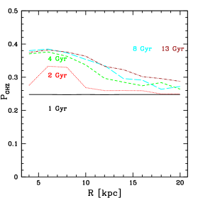
Figure 3: The probability $P_{GHZ}(R,t)$ as a function of the galactocentric distance of having Earths where the effects of SN explosions are not considered for the classical model S2IT at 1, 2, 4, 8, 13 Gyr.

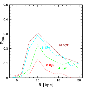
Figure 4: The probability $P_{GHZ}(R,t)$ as a function of the galactocentric distance of having Earths where the case 2) of SN explosions are considered for the classical model S2IT at 1, 2, 4, 8, 13 Gyr.

Figure 5: A comparison between the SN rate histories at 8 and 20 kpc for the model S2IT.

3.1 The Milky Way (S2IT model)

To follow the chemical evolution of the Milky Way without radial flows of gas, we adopt the model S2IT of Spitoni & Matteucci (2011) which is an updated version of the two infall model Chiappini et al. (1997) model. This model assumes that the halo-thick disk forms out of an infall episode independent of that which formed the disk. In particular, the assumed infall law is

$$A(r,t)=a(r)e^{-t/\tau_{H}}+b(r)e^{-(t-t_{max})/\tau_{D}(r)},$$ (6)

where $\tau_{H}$ is the typical timescale for the formation of the halo and thick disk is 0.8 Gyr, while $t_{max}$ = 1 Gyr is the time for the maximum infall on the thin disk. The coefficients $a(r)$ and $b(r)$ are obtained by imposing a fit to the observed current total surface mass density in the thin disk as a function of galactocentric distance given by:

$$\Sigma(r)=\Sigma_{0}e^{-R/R_{D}},$$ (7)

where $\Sigma_{0}$ = 531 M pc^-2 is the central total surface mass density and $R_{D}$ = 3.5 kpc is the scale length.

Moreover, the formation timescale of the thin disk is assumed to be a function of the Galactocentric distance, leading to an inside-out scenario for the Galaxy disk build-up. The Galactic thin disk is approximated by several independent rings, 2 kpc wide, without exchange of matter between them.

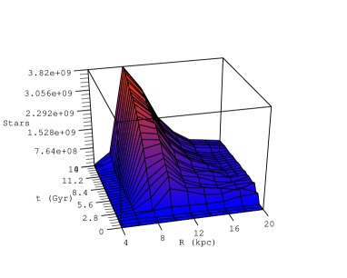
Figure 6: The total number of stars having Earths ($N_{\star life}$) as a function of the Galactocentric distance and the Galactic time where the case 2) of SN explosions are considered for the classical model S2IT. The ($N_{\star life}$) values are computed within concentric rings, 2 kpc wide.

A threshold gas density of 7 M_⊙ pc^-2 in the SF process (Kennicutt 1989, 1998; Martin & Kennicutt 2001; Schaye 2004) is also adopted for the disk. The halo has a constant surface mass density as a function of the galactocentric distance at the present time equal to 17 M_⊙ pc^-2 and a threshold for the star formation in the halo phase of 4 M_⊙ pc^-2, as assumed for the model B of Chiappini et al. (2001).

The assumed IMF is the one of Scalo (1986), which is assumed constant in time and space. The adopted law for the SFR is a Schmidt (1958) like one:

$$\Psi\propto\nu\Sigma^{k}_{gas}(r,t),$$ (8)

where $\Sigma_{gas}(r,t)$ is the surface gas density with the exponent $k$ equal to 1.5 (see Kennicutt 1998; and Chiappini et al. 1997). The quantity $\nu$ is the efficiency of the star formation process, and it is constant and fixed to be equal to 1 Gyr ^-1.

In Table 1 the principal characteristics of the S2IT model are reported: in the second column the infall type is reported, in the third and forth ones the time scale $\tau_{d}$ of the thin disk formation, and the time scale $\tau_{H}$ of the halo formation are drawn. The dependence of $\tau_{d}$ on the Galactocentric distance $R$, as required by the inside-out formation scenario, is expressed in the following relation:

$$\tau_{d}=1.033R\mbox{[kpc]}-1.27\mbox{ [Gyr]}.$$ (9)

is in column 5. The adopted threshold in the surface gas density for the star formation, and total surface mass density for the halo are reported in column 6 and 7, respectively.

In the left panel of Fig. 2 the surface density profile for the stars as predicted by the model S2IT is reported. Observational data are the ones used by Chiappini et al. (2001).

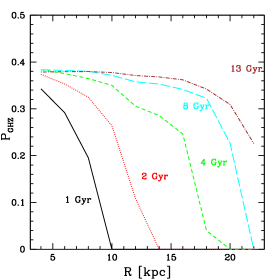
Figure 7: The probability $P_{GHZ}(R,t)$ as a function of the galactocentric distance of having Earths where the effects of SN explosions are not considered for the classical model M31B at 1, 2, 4, 8, 13 Gyr.

3.2 M31 (M31B model)

To reproduce the chemical evolution of M31, we adopt the best model M31B of Spitoni et al. (2013). The surface mass density distribution is assumed to be exponential with the scale-length radius $R_{D}=5.4$ kpc and central surface density $\Sigma_{0}=460M_{\odot}pc^{-2}$, as suggested by Geehan et al. (2006). It is a one infall model with inside-out formation, in other words we consider only the formation of the disk. The time scale for the infalling gas is a function of the Galactocentric radius: $\tau(R)=0.62R+1.62$. The disk is divided in several shells 2 kpc wide as for the Milky Way.

In order to reproduce the gas distribution they adopted for the model M31B the SFR of eq. (8) with the following star formation efficiency: $\nu(R)=24/R-1.5$, until it reaches a minimum value of 0.5 Gyr^-1 and then is assumed to be constant. Finally, a threshold in gas density for star formation of 5 $M_{\odot}/pc^{2}$ is considered, as suggested in Braun et al. (2009). The model parameters for the time scale of the infalling gas, for the star formation efficiency, and for the threshold are summarized in Table 2. The assumed IMF is the one of Kroupa et al. (1993).

Our reference model of M31 overestimates the present-day SFR data. In fact, our “classical” model is similar to that of Marcon-Uchida et al. (2010). The same model, however, well reproduces the oxygen abundance along the M31 disk. We think that more uncertainties are present in the derivation of the star formation rate than in the abundances.

4 The chemical evolution models with radial flows of gas

In this section we present the best models in presence of radial gas flows we will use in this work. For the Milky Way our reference radial gas flow model is the “RD” of Mott et al. (2013), whereas for M31 we refer to the model “M31R” we proposed in Spitoni et al. (2013).

4.1 The Milky Way (RD model)

We consider here the best model RD presented by Mott et al. (2013) to describe the chemical evolution of the Galactic disk in presence of radial flows. From Table 1 we see that this model shows the same prescriptions of the S2IT model for the inside-out formation and for the SFR efficiency fixed at 1 Gyr^-1. On the other hand the RD model has not a threshold in the SF and a different modeling of the surface density for the halo was used: the total surface mass density in the halo $\sigma_{H}(R)$ becoming very small for distances $\geq$ 10 kpc, a more realistic situation than that in model S2IT.

The radial flow velocity pattern is shown in Fig. 2 labeled as “pattern III”. The range of velocities span between 0 and 3.6 km s^-1.

We recall here that in the implementation of the radial inflow of gas in the Milky Way, presented by Mott et al. (2013), only the gas that resides inside the Galactic disk within the radius of 20 kpc can move inward by radial inflow, and as a boundary condition we impose that there is no flow of gas from regions outside the ring centered at 20 kpc.

In the left panel of Fig. 2 the surface density profile for the stars predicted by the model RD is reported. Observational data are the ones used by Chiappini et al. (2001).

4.2 M31 (M31R model)

M31R is the best model for M31 in presence of radial flows presented by Spitoni et al. (2013). It assumes a constant star formation efficiency, fixed at the value of 2 Gyr^-1 and, it does not include a star formation threshold.

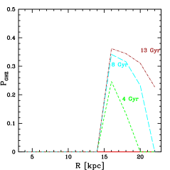
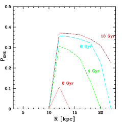
Figure 8: The probability $P_{GHZ}(R,t)$ as a function of the galactocentric distance of having Earth-like planets for the classical model M31B at 1, 2, 4, 8, 13 Gyr including the case 1) SN explosions effects in the left panel. The results for the same model but with the case 2) prescription for the SN destruction are drawn in the right panel.

At variance with the RD model, where the radial flows was applied to a two-infall model, for the M31R model it was possible to find a linear velocity pattern as a function of the galactocentric distance.

The radial inflow velocity pattern requested to reproduce the data follows this linear relation:

$$v_{R}=0.05R[\mbox{kpc}]+0.45\mbox{ }[\mbox{km s}^{-1}],$$ (10)

and spans the range of velocities between 1.55 and 0.65 km s^-1 as shown in Fig. 2.

Therefore in the external regions the velocity inflow for the Milky Way model is higher than the M31 velocity flows as shown in Fig. 2. At 20 kpc the ratio between the inflow velocities is $v_{RD}/v_{M31R}\simeq 2.5$.

The model M31R fits the O abundance gradient in the disk of M31 very well. The other model parameters are reported in Table 2.

We recall here that in the implementation of the radial inflow of gas in M31 presented by Spitoni et al. (2013), only the gas that resides inside the Galactic disk within the radius of 22 kpc can move inward by radial inflow, and as boundary condition we impose that there is no flow of gas from regions outside the ring centered at 22 kpc, as already discussed for the Milky Way.

5 The Classical model GHZ results

In this section we report our results concerning the GHZ using “classical” chemical evolution models.

5.1 The Milky Way model results

We start to present the Milky Way results for the models without any radial flow of gas. In Fig. 3 the probability $P_{GHZ}(R,t)$ for the model S2IT of our Galaxy without the effects of SN are reported, at 1, 2, 4, 8, 13 Gyr. We recall that S2IT is a two infall model. Comparing Table 1 with Table 2 we notice another important difference between the S2IT and M31B models. For the Milky Way the star formation efficiency $\nu$ is constant and taken equal to 1 Gyr^-1 whereas for M31 is $\nu$= 24/(R[kpc])-1.5. This is the reason why our results are different from the Prantzos (2008) ones. In fact the reference chemical evolution model for the Milky Way in Prantzos (2008) is the one described in Boissier & Prantzos (1999), where the SFR is $\propto R^{-1}$. Hence at variance with the Prantzos (2008) GHZ results, the probability that a star has a planet with life is high also in the external regions at the early times. At 1 Gyr we notice that the $P_{GHZ}$ values are constant along the disk. The reason for that resides in the fact that in the first Gyr the SFR is the same at all radii, since it reflects the SF in the halo (see Fig.1 of Spitoni et al. 2009).

For our Galaxy we just show the results of the SN case 2) model reported in Fig. 4. This is our best model for the Milky Way considering our SN rate history. With this model the region with the highest probability that a formed star can host a Earth-like planet with life is between 8 and 12 kpc, and the maximum located at 10 kpc.

The Milky Way outer parts are affected by the SN destruction: in fact, the predicted SN rate using Galaxy evolution as time goes by can overcome the value fixed by the case 2): $2\times<RSN_{SV}>$, and consequently $P_{GHZ}$ drops down.

This is shown in Fig. 5 where the SN rates at 8 and 20 kpc are reported for our Galaxy.

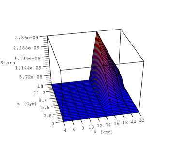
Figure 9: The total number of stars having Earths ($N_{\star life}$) as a function of the galactocentric distance and the galactic time including the effects of SN explosions described by the case 1) prescription for the classical model M31B. The ($N_{\star life}$) values are computed within concentric rings, 2 kpc wide.

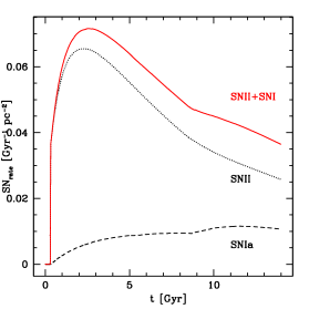
Figure 10: The Type Ia and II SN rates expressed in pc^-2 Gyr^-1 as a function of the galactic time (Gyr), as predicted by the classical model M31B for Andromeda of Spitoni et al. (2013) at 8 kpc.

In Fig. 4 it is shown that the probability $P_{GHZ}$ increases in the outer regions as time goes by, in agreement with the previous works of of Lineweaver et al. (2004) and Prantzos (2008). In both works it was also found that the peak of the maximum probability moves outwards with time. With our chemical evolution model such an effect is not present, and the peak is always located at the 10 kpc from the Galactic center. This effect is probably due to the balance of the destruction by SNe and SFR occurring at this distance.

In Fig. 6 we present our results concerning the quantity $N_{\star life}$, i.e. total number of stars as a function of the Galactic time and the Galactocentric distance for the model S2IT in presence of the SN destruction effect (case 2). As found by Prantzos (2008) the GHZ, expressed in terms of the total number of host stars peaks at galactocentric distances smaller than in the case in which are considered the fraction of stars (eq. 3). This is due to the fact that in the external regions the number of stars formed at any time is smaller than in the inner regions. In fact, the maximum numbers of host stars peaks at 8 kpc whereas the maximum fraction of stars peaks at 10 kpc (see Fig. 4). Our results are in perfect agreement with Lineweaver et al. (2004) who identified for the Milky Way the GHZ as an annular region between 7 and 9 kpc from the Galactic center that widens with time.

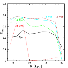
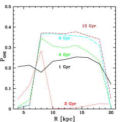
Figure 11: Left panel: The probability $P_{GHZ}(R,t)$ as a function of the galactocentric distance of having Earths where the effects of SN explosions are not considered for the Milky Way model RD with radial gas flows at 1, 2, 4, 8, 13 Gyr. Right panel: The probability $P_{GHZ}(R,t)$ as a function of the galactocentric distance of having Earths including the effects of SN explosions of the case 2) prescription for The Milky Way model RD with radial gas flows at 1, 2, 4, 8, 13 Gyr.

5.2 M31 model results

In Fig. 7 we show the probability $P_{GHZ}(R,t)$ as a function of the galactocentric distance of having Earths where the effects of SN explosions are not considered, for the classical model M31B at 1, 2, 4, 8, 13 Gyr.

The shape and evolution in time of the $P_{GHZ}(R,t)$ for M31 is similar to the one found by Prantzos (2008) for the Milky Way.

The similar behavior is due to the choice of similar prescriptions for the SFR. In fact for M31, as it can be inferred in Table 2, we have a similar law for the SFR, in fact our SF efficiency is a function of the galactocentric distance with the following law: $\nu$= 24/(R[kpc])-1.5.

In Fig. 7 we can see that as time goes by non-negligible $P_{GHZ}$ values extend to the external parts of Galaxy. Early on, at 1 Gyr non zero values of $P_{GHZ}$ can be found just in the inner regions for distances smaller than 10 kpc from the galactic center. In this plot, it can be visualized the gradual extension of the fraction of stars with habitable planets up to the outer regions, during the galactic time evolution.

The GHZ for the classical model of M31 taking into account case 1) for the SN destruction effects, is reported in the left panel of Fig. 8.

Comparing our results with the ones of Carigi et al. (2013) with the same prescriptions for the SN destruction effect (their Fig. 6, first upper panels), we find that substantial differences in the inner regions (R $\leq$ 14 kpc): at variance with that paper we have a high enough SN rate to annihilate the life on formed planets. In Fig. 9, where the total number of stars having Earths ($N_{\star life}$) is reported, it is clearly shown that the region with no host stars spans all galactocentric distances smaller or equal than 14 kpc during the entire galactic evolution. On the other hand, the two model are in very good agreement for the external regions.

We have to remind that at variance with our models, the Carigi et al. (2013) one is not able to follow the evolution of [Fe/H], because they did not consider Type Ia SN explosions.

In the total budget of the SN rate they did not consider the SN Type Ia. In Fig. 10 we show the contribution of Type Ia SN rate expressed in Gyr^-1 pc^-2 for the M31B model at 8 kpc. We note that it is not negligible and it must be taken into account for a correct description of the chemical evolution of the galaxy.

It is fair to recall here that our model M31B overestimates the present-day SFR. Therefore, we are aware that in recent time there could have been favorable conditions for the growth of the life as found in Carigi et al. (2013) work also in regions at Galactocentric distances $R\leq 14$. Anyway, as stated by Renda (2005) and Yin et al. (2009), the Andromeda galaxy had an overall higher star formation efficiency than the Milky Way. Hence, during the galactic history the higher SFR had probably led to not favorable condition for the life.

The case 2) model is reported in the right panel of Fig. 8. As expected, the habitable zone region increases in the inner regions, reaching non-zero values for radius $>10$ kpc.

At variance with case 2) for S2IT model, we see that the external regions are not affected by the SN destruction. In fact, the SF efficiency is lower in the external regions when compared with those of the Milky Way. Moreover, the SN rates from the galaxy evolution of M31 are always below the value fixed by the case 2): $2\times<RSN_{SV}>$, and consequently $P_{GHZ}$ does not change.

6 Radial flows GHZ results

We pass now to analyze our results concerning both M31 and our Galaxy in presence of radial flow of gas.

6.1 The Milky Way model results in presence of radial flows

In the left panel of Fig. 11 the RD model results without SN destruction are presented. Although the RD model does not include any threshold in the SF, at 20 kpc we note a deep drop in the probability $P_{GHZ}(R,t)$, at variance with what we have shown for the “classical” model S2IT without SN effects (Fig. 3).

Figure 12: Left: Upper panel: [Fe/H] as a function of the Galactic time for the model RD at 20 kpc. The lower limit in the [Fe/H] is fixed at -1 dex. Below this values the probability of forming Earth-like planets ($P_{FE}$) is zero. Lower panel: Star formation rate history for the Galaxy for the model RD at 20 kpc. Right: the same quantities are plotted for the S2IT model at 20 kpc.

The explanation can be found in Fig. 2: in the outer parts of the Galaxy the inflow velocities are roughly 2.5 times larger than the M31 ones, creating a tremendous drop in the SF. In Fig. 12 we report the SFR and [Fe/H] histories at 20 kpc for RD and S2IT models respectively. For the [Fe/H] plot we fixed the lower limit at -1 dex, because this is the threshold for the creation of habitable planets.

Figure 13: Upper panel: [Fe/H] as a function of the Galactic time for the model RD at 10 kpc. The lower limit in the [Fe/H] is fixed at -1 dex. Below this values the probability of forming Earth-like planets ($P_{FE}$) is zero. Lower panel: Star formation rate history for the Galaxy for the model RD at 10 kpc.

Concerning the RD model the high inflow velocity has the effect of removing a not negligible amount of gas from the shell centered at 20 kpc (the outermost shell for the Milky Way model). In the left lower panel of Fig. 12 we see that the maximum value of the SFR for the RD model is 0.01 M_⊙ pc^-2 Gyr^-1. It is important also to recall here that in the RD model for Galactocentric distances $\geq$ 10 kpc a constant surface mass density of $\sigma_{H}$ 0.01 M_⊙ pc^-2 Gyr^-1 is considered for the halo, at variance with the model S2IT where it has been fixed at 17 M_⊙ pc^-2 Gyr^-1.

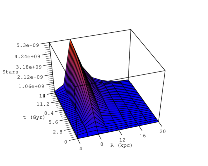
Figure 14: The total number of stars having Earths ($N_{\star life}$) as a function of the Galactocentric distance and the Galactic time including the effects of SN explosions described by the case 2) prescription for the Milky Way model with gas radial flows (RD model). The ($N_{\star life}$) values are computed within concentric rings, 2 kpc wide.

The $P_{GHZ}$ value depends on the product of the [Fe/H] and SFR quantities. Because the RD model at 20 kpc shows [Fe/H] $>$ -1 in small ranges of time ($0.6<t<1$ Gyr and $t>10.3$ Gyr), we find very small values for $P_{GHZ}$ during the whole Galactic history.

In the right side of Fig. 12 the different behavior of the model S2IT at 20 kpc is reported. In this case even if there is a threshold in the star formation we have [Fe/H] $>$ -1 dex at all times, and the SFR when is not zero is also 800 times higher than in the RD model. This is why in Fig. 3 the model S2IT shows higher values of $P_{GHZ}$ at 20 kpc.

We discuss now the probability $P_{GHZ}(R,t)$ at 2 Gyr in the model RD. It drops almost to zero for galactocentric distances $\geq$ 10 kpc. In Fig. 13 we report the SFR and [Fe/H] histories for the model RD at 10 kpc. We recall that in the model RD the halo surface density is really small for $R\geq 10$ kpc (0.01 M_⊙ pc^-2 Gyr^-1).

We can estimate the $P_{GHZ}$(10 kpc, 2 Gyr) value obtained with eq. (4) using simple approximated analytical calculations. For the numerator we note that in the interval of time between 0 and 2 Gyr, [Fe/H] $>$ -1 dex only approximately in the range 0.5, 1 Gyr, where $P_{E}$=0.4. In the lower panel of Fig. 13 it is shown that for this interval the SFR value. is roughly constant and $\simeq 4\times 10^{-4}$ M_⊙ pc^-2 Gyr^-1.

Hence, we can approximate the numerator integral as:

$$N\,\! = \!\,\int_{0}^{2Gyr}SFR\times P_{E}\,\,dt^{\prime}$$ (11)

$$\simeq \!\,\int_{0.5Gyr}^{1Gyr}4\times 10^{-3}\times 0.4\,\,dt^{\prime}=0.8\times 10^{-3}.$$

The denominator of eq. (4) is

$$D=\int_{0}^{2Gyr}SFR\times P_{E}\,\,dt^{\prime}.$$ (12)

The integral of the SFR is negligible in the first Gyr compared with the one computed in the interval between 1 and 2 Gyr. A lower limit estimate of D is given by:

$$D\simeq\int_{1Gyr}^{2Gyr}SFR\times P_{E}\,\,dt^{\prime}\geq(1.36)\times 0.5=0.9,$$ (13)

where a linear growth of the SFR from 0 to 1.35 M_⊙ pc^-2 Gyr^-1 in the interval 1-2 Gyr was considered in reference of the Fig. 13.

Finally, the approximated $P_{GHZ}$(10 kpc, 2 Gyr) value is:

$$\frac{N}{D}\simeq 0.9\times 10^{-3}.$$ (14)

Our numerical result is in perfect agreement with this lower limit approximation, in fact numerically we obtain $P_{GHZ}$(10 kpc, 2 Gyr)= 1.12609298 $\times 10^{-3}$.

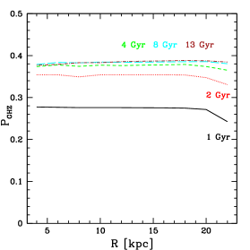
Figure 15: The probability $P_{GHZ}(R,t)$ as a function of the galactocentric distance of having Earths where the effects of SN explosions are not considered for the model M31R with radial gas flows at 1, 2, 4, 8, 13 Gyr.

Here again, as done for the Milky Way “classical” model, we report the results for the best model in presence of SN destruction which is capable to predict the existence of stars hosting Earth-like planets in the solar neighborhood. The SN destruction case 2) gives again the best results (see Fig. 11). We notice that the external regions are not affected from the SN destruction at variance with what we have seen above for the “classical” model S2IT.

Comparing the “classical” model of Fig. 4 with the right panel of Fig. 11 we see that for the Milky Way the main effect of a radial inflow of gas is to enhance the probability $P_{GHZ}$ in outer regions when the supernova destruction are also taken into account.

In Fig. 14 the quantity $N_{\star life}$ is drawn for the RD model. We see that the region with the maximum number of host stars centers at 8 kpc, and that this number decreases toward the external regions of the Galaxy. The reason for this is shown in the right panel of Fig. 2: in the RD model the radial inflow of gas is strong enough in the external parts of the Milky Way to lower the number of stars formed. Hence, although the probability $P_{GHZ}$ is still high in at large Galactocentric distances, the total number of the stars formed is smaller during the entire Galactic history compared to the internal Galactic regions. At the present time, at 8 kpc the total number of host stars is increased by 38 % compared to the S2IT model results.

6.2 M31 model results in presence of radial flows

The last results are related to the GHZ of M31 in presence of radial flows of gas. In Fig. 15 we report the probability $P_{GHZ}(R,t)$ of having Earths without the effects of SN explosions for the model M31R at 1, 2, 4, 8, 13 Gyr. The main effect of the gas radial inflow with the velocity pattern of eq. (10), is to enhance at anytime the probability to find a planet with life around a star in outer regions of the galaxy compared to the classical result reported in Fig. 7 also when the destruction effect of SN is not taken into account.

This behavior is due to two main reasons: 1) the M31R model has a constant SFR efficiency as a function of the galactocentric distances, this means higher SFR in the external regions; 2) the radial inflow velocities are small in the outer part of M31 compared to the one used for the Milky Way model RD (see Fig. 2), therefore the gas removed from the outer shell in the M31R model (the one centered at 22 kpc) is very small. In fact, in Fig. 15 the drop in the $P_{GHZ}(R,t)$ quantity at 22 kpc is almost negligible if compared to the one reported in Fig. 11 for the RD model of the Milky Way, described in the Section 6.1.

For the M31R model with radial flows we will show just the results with the case 1) with SN destruction.

In Fig. 16 the effects of the case 1) SN destruction on the M31R model are shown. The external regions for galactocentric distances $\geq$ 16 kpc are not affected by SNe, on the other hand for radii $<$ 14 kpc due to the higher SNR relative to $<RSN_{SV}>$, there are not the condition to create Earth-like planets at during whole the galactic time. In Fig. 17 the total number of host stars $N_{\star life}$ are shown. Also in this case, in the external parts the total number of stars formed and consequently the ones hosting habitable planets are small compared to the inner regions. The galactocentric distance with the maximum number of host stars is 16 kpc. Presently, at this distance the total number of host stars $N_{\star life}$ is increased by 10 % compared to the M31B model results.

Comparing Fig. 17 with Fig. 9 we note that at variance with the Milky Way results the $N_{\star life}$ value for the M31R model is always higher compared to the M31B results. This is due to the slower inflow of gas and the constant star formation efficiency which favor the formation of more stars.

For the case 2), we just mention that as expected the GHZ is wider than the case 1) described above and for radii $<$ 12 kpc, there are not the condition to create Earth-like planets at during whole the galactic time.

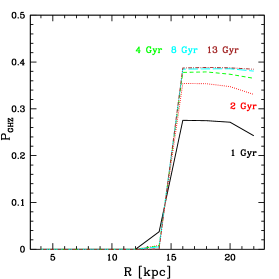
Figure 16: The probability $P_{GHZ}(R,t)$ as a function of the galactocentric distance of having Earths including the effects of SN explosions of the case 1) prescription for the model M31R with radial gas flows at 1, 2, 4, 8, 13 Gyr.

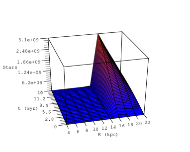
Figure 17: The total number of stars having Earths ($N_{\star life}$) as a function of the galactocentric distance and the galactic time including the effects of SN explosions described by the case 1) prescription for the model M31R with gas radial flows. The ($N_{\star life}$) values are computed within concentric rings, 2 kpc wide.

7 Conclusions

In this paper we computed the habitable zones (GHZs) for our Galaxy and M31 systems, taking into account “classical” models and models with radial gas inflows. We summarize here our main results presented in the previous Sections. Concerning the “classical” models we obtained:

• The Milky Way model which is in agreement with the work of Lineweaver et al. (2004) assumes the case 2) for the SN destruction (the SN destruction is effective if the SN rate at any time and at any radius is higher than two times the average SN rate in the solar neighborhood during the last 4.5 Gyr of the Milky Way’s life). With this assumption, we find that the Galactic region with the highest number of host stars of an Earth-like planet is between 7 and 9 kpc with the maximum localized at 8 kpc.

• For Andromeda, comparing our results with the ones of Carigi et al. (2013), with the same prescriptions for the SN destruction effects, we find substantial differences in the inner regions (R $\leq$ 14 kpc). In particular, in this region there is a high enough SN rate to annihilate life on formed planets at variance with Carigi et al. (2013). Nevertheless, we are in agreement for the external regions. It is important to stress the most important limit of the Carigi et al. (2013) model: Type Ia SN explosions were not considered. We have shown instead, that this quantity is important both for Andromeda and for the Galaxy.

In this work for the first time the effects of radial flows of gas were tested on the GHZ evolution, in the framework of chemical evolution models.

• Concerning the models with radial gas flows both for the Milky Way and M31 the effect of the gas radial inflows is to enhance the number of stars hosting a habitable planet with respect to the “classical” model results in the region of maximum probability for this occurrence, relative to the classical model results.

  In more details we found that:

• At the present time, for the Milky Way if we treat the SN destruction effect following the case 2) criteria, the total number of host stars as a function of the Galactic time and Galactocentric distance tell us that the maximum number of stars is centered at 8 kpc, and the total number of host stars is increased by 38 % compared to the “classical” model results.

• In M31 the main effect of the gas radial inflow is to enhance at anytime the fraction of stars with habitable planets, described by the probability $P_{GHZ}$, in outer regions compared to the classical model results also for the models without SN destruction. This is due to the fact that: i) the M31R model has a fixed SFR efficiency throughout all the galactocentric distances, this means that in the external regions there is a higher SFR compared to the “classical” M31B model; ii) the radial inflow velocities are smaller in the outer part of the galaxy compared to the ones used for the Milky Way model RD, therefore not so much gas is removed from the outer shell. The galactocentric distance with the maximum number of host stars is 16 kpc. Presently, at this distance the total number of host stars is increased by 10 % compared to the M31B model results. These values for the M31R model are always higher than the M31B ones.

  In spite of the fact that in in the future it will be very unlikely to observe habitable planets in M31, that could confirm these model results about the GHZ, our aim here was to test how GHZ models change in accordance with different types of spiral galaxies, and different chemical evolution prescriptions.

References

- Boissier (1999) Boissier S., Prantzos N., 1999, MNRAS, 307, 857
- Bonfils (2013) Bonfils, X., Lo Curto, G., Correia, A. C. M., Laskar, J., Udry, S., Delfosse, X., Forveille, T., Astudillo-Defru, N., Benz, W., Bouchy, F., et al., 2013, A&A, 556, A110
- Braun (2009) Braun, R., Thilker, D. A., Walterbos, R. A. M., & Corbelli, E. 2009, ApJ, 695, 937
- Buchhave (2012) Buchhave, L. A., Latham, D. W., Johansen, A., Bizzarro, M., Torres, G., Rowe, J. F., Batalha, N. M., Borucki, W. J., Brugamyer, E., Caldwell, C., et al., 2012, Nature, 486, 375
- Carigi (2013) Carigi, L., Garcia-Rojas, J., Meneses-Goytia, S., 2013, RMAA, 49, 253
- Chiappini (1997) Chiappini, C., Matteucci, F., & Gratton, R. 1997, ApJ, 477, 765
- Chiappini (2001) Chiappini, C., Matteucci, F., & Romano, D. 2001, ApJ, 554, 1044
- Dressing (2013) Dressing, C. D., Charbonneau, D., 2013, ApJ, 767,95
- Fischer (2005) Fischer, D., A., Valenti, J., 2005, ApJ, 622,1102
- Geehan (2006) Geehan, J. J., Fardal, M. A., Babul, A., & Guhathakurta, P. 2006, MNRAS, 366, 996
- Scalo (1986) Gonzalez, G. 1997, MNRAS, 285, 403
- Gonzalez (2001) Gonzalez, G., Brownlee, D., Ward, P. 2001, Icarus, 152, 185
- Hart (1979) Hart, M. H. 1979, Icarus 37, 351-357.
- Huang (1959) Huang, S.-S. 1959, American Scientist 47, 397-402.
- Johnson (2012) Johnson, J. L., Li, H., 2012, ApJ, 751, 81
- Kasting (1993) Kasting, J. F., Whitmire, D. P., Reynolds, R. T., 1993, Icarus, 101,108
- Kennicutt (1989) Kennicutt, R. C., Jr. 1989, ApJ, 344, 685
- Kennicutt (1998) Kennicutt, R. C., Jr. 1998, ApJ, 498, 541
- Kroupa (1993) Kroupa, P., Tout, C. A., & Gilmore, G. 1993, MNRAS, 262, 545
- Kubryk (2013) Kubryk, M., Prantzos, N., Athanassoula, E., 2013, MNRAS, 436, 1479
- Lineweaver (2001) Lineweaver, C. H., 2001, Icarus, 151, 307
- Lineweaver (2004) Lineweaver, C. H., Fenner, Y., Gibson, B. K., 2004, Science, 303, 59
- Marcon (2010) Marcon-Uchida, M. M., Matteucci, F., Costa, R. D. D., 2010, A&A, 520, A35
- Martin (2001) Martin, C. L., & Kennicutt, R. C., Jr. 2001, ApJ, 555, 301
- McMahon (2013) McMahon, S., O’Malley-James, J., Parnell, J., 2013, P&SS, 85, 312
- Minchev (2013) Minchev, I., Chiappini, C., Martig, M., 2013, A&A, 558, A9
- Mortier (2013a) Mortier, A., Santos, N. C., Sousa, S. G., Fernandes, J. M., Adibekyan, V. Zh., Delgado Mena, E., Montalto, M., Israelian, G., 2013a, 558, A106
- Mortier (2013b) Mortier, A.; Santos, N. C.; Sousa, S.; Israelian, G.; Mayor, M.; Udry, S., 2013b, 557, A70
- Mott (2013) Mott, A., Spitoni, E., Matteucci, F., 2013, MNRAS, 435, 2918,
- Petigura (2013) Petigura, E. A., Howard, A. W., Marcy, G. W., 2013, PNAS, 110, 19175
- Prantzos (2008) Prantzos, N. 2008, Space Sci. Rev., 135, 313
- Renda (2005) Renda, A., Kawata, D., Fenner, Y., Gibson, B. K. 2005, MNRAS, 356, 1071
- santos (2001) Santos, N. C., Israelian, G., & Mayor, M. 2001, A&A, 373, 1019
- santos (2004) Santos, N. C., Israelian, G., & Mayor, M. 2004, A&A, 415, 1153
- Scalo (1986) Scalo, J. M. 1986, FCPh, 11, 1
- Schaye (2004) Schaye, J. 2004, ApJ, 609, 667
- Selsis (2007) Selsis, F., Kasting, J. F., Levrard, B., Paillet, J., Ribas, I., Delfosse, X., 2007, A&A, 467, 1373
- Shklovski (1966) Shklovski, I. S., and Sagan, C., 1966, Intelligent Life in the Universe, San Francisco: Holden-Day
- Sousa (2011) Sousa, S. G., Santos, Israelian, G., Mayor, M., Udry, S., 2011, A&A, 533, A141
- Sozzetti (2009) Sozzetti, A., Torres, G., Latham, David W., Stefanik, R. P., Korzennik, S. G., Boss, A. P., Carney, B. W., Laird, J. B., 2009, ApJ, 697,544
- Spitoni (2011) Spitoni, E., & Matteucci, F. 2011, A&A, 531, A72
- Spitoni (2011) Spitoni, E., Matteucci, F., Marcon-Uchida, M. M., 2013, A&A, 551, A123
- Spitoni (2009) Spitoni, E., Matteucci, F., Recchi, S., Cescutti, G., Pipino, A. 2009, A&A, 504, 87
- Tarter (2007) Tarter, J. C., Backus, P. R., Mancinelli, R. L., Aurnou, J. M., Backman, D. E., Basri, G. S., Boss, A. P., Clarke, A., Deming, D., Doyle, L. R., et al., 2007, AsBio, 7 ,30
- udry (2006) Udry, S., Mayor, M., Benz, W., et al. 2006, A&A, 447, 361
- Udry (2007) Udry, S. & Santos, N. C. 2007, ARA&A, 45, 397
- Underwood (2003) Underwood, D. R., Jones, B. W., Sleep, P. N., 2003, IJAsb, 2, 289
- Vladilo (2013) Vladilo G., Murante G., Silva L., Provenzale A., Ferri G., Ragazzini G., 2013, ApJ, 767, 65
- Yin (2009) Yin, J., Hou, J. L., Prantzos, N., Boissier, S., Chang, R. X., Shen, S. Y., Zhang, B., 2009, A&A, 505, 508