Chiral selection and frequency response of spiral waves in reaction-diffusion systems under a chiral electric field

Abstract

Chirality is one of the most fundamental properties of many physical, chemical and biological systems. However, the mechanisms underlying the onset and control of chiral symmetry are largely understudied. We investigate possibility of chirality control in a chemical excitable system (the BZ reaction) by application of a chiral (rotating) electric field using the Oregonator model. We find that unlike previous findings, we can achieve the chirality control not only in the field rotation direction, but also opposite to it, depending on the field rotation frequency. To unravel the mechanism, we further develop a comprehensive theory of frequency synchronization based on the response function approach. We find that this problem can be described by the Adler equation and show phase-locking phenomena, known as the Arnold tongue. Our theoretical predictions are in good quantitative agreement with the numerical simulations and provide a solid basis for chirality control in excitable media.

I Introduction

Chirality is a significant property of asymmetry that has been found in several branches of science with notorious examples in fields ranging from particle physics to biological systems wagniere . In the context of pattern formation, a typical self-organized wave pattern bearing chirality is a spiral wave, as it has topological charge (either -1 or +1) that is related to the sense of rotation, e.g., clockwise (CW) or counterclockwise (CCW). Spiral waves have been found in a wide variety of chemical, physical and biological systems. For instance, they occur in the classical Belousov-Zhabotinsky (BZ) reaction win72 ; ouy96 ; van01 , on platinum surfaces during the process of catalytic oxidation of carbon monoxide jak90 , in the liquid crystal frisch , during aggregation of Dictyostelium discoideum amoebae lee96 , in the chicken retina yu12 and in cardiac tissue where they are thought to lead to life-threatening cardiac arrhythmias dav92 .

To date, much attention has been paid to spiral dynamics as they respond to various external fields such as dc and ac electric fields agladze_elc_jpc ; steinbock_elc_prl ; krinsky_elc_prl ; taboada ; schmidt ; munuzuri94 , periodic forcing steibocknat ; Braunecpl ; mantelpre ; linprl ; zhangprl , mechanical deformation munuzuri_elc_pre ; sasha ; daniel , and heterogeneity zoupre93 ; hans ; biktashevprl10 ; bwlicol ; alonsoprl ; defauw . As reaction-diffusion (RD) systems exhibit mirror symmetry, CCW and CW spiral waves are physically identical and the response of spiral waves with opposite chirality to achiral fields is identical up to mirror symmetry. For example, the sense of drift perpendicular to a constant electric field will change for a spiral wave of opposite chirality agladze_elc_jpc ; steinbock_elc_prl ; krinsky_elc_prl . The chiral property of spiral waves causes some interesting behaviors, in particular as they respond to a chiral field nicolis_pnas ; miglerprl ; knam ; ecke_sci . However this issue to our best knowledge remains to be comparatively less addressed over last decades. Recently, a circularly polarized electric field (CPEF) that possesses chirality was theoretically proposed chenjcp1 and was implemented in the BZ experiment jipre , which allows us to study the response of spiral waves to a chiral electric field in RD systems. Indeed, it has been shown that the CPEF has some pronounce effects on spiral waves chenjcp2 ; caimc ; bwli13 that were not observed in RD systems subject to achiral fields such as a dc or ac electric field.

Possibly, one of the most interesting results caused by chiral fields or forces is chiral symmetry breaking, an ubiquitously observed scenario in nature ecke_sci ; miglerprl ; nicolis_pnas ; carmichael ; ricci ; ribo ; noorduin ; toyoda . Over the past decades, chiral symmetry breaking induced by such chiral fields has received considerable interests from many scientific disciplines ecke_sci ; miglerprl ; nicolis_pnas ; ribo ; noorduin ; toyoda . Different from spontaneous chiral symmetry breaking where the chiral selection is unpredicted, it was demonstrated that chiral fields not only cause the breaking of chirality but also could select a desired chiralityecke_sci ; miglerprl ; nicolis_pnas ; ribo ; noorduin ; toyoda , which is closely related with that of the applied field. As an example, the chirality of a supramolecular structure can be selected by the vortex motion and depends on the chirality of the vortex ribo . In Rayleigh-Bénard convection, chiral symmetry breaking in spiral-defect populations was observed when the system rotated along the vertical axis, and the chirality of the dominant spirals relies on the rotation sense of the system ecke_sci . By subjecting a RD system to the CPEF bwli13 , we recently found that the zero-rotation chiral symmetry between CW and CCW spiral defects breaks and that ordered spiral waves with preferred chirality arise from the spiral turbulence state. Here too, the preferred chirality was only determined by the chirality of the CPEF bwli13 .

On the other hand, due to the presence of chiral terms, the frequency response of spiral waves with opposite chirality is different. For example, in the complex Ginzburg-Laudau equation (CGLE) with a broken chiral symmetry breaking term, Nam et al. knam showed that this chiral term would cause a shift in the frequency of spiral waves and the sign of this shift depends on the chirality of the spiral waves. In our recent work bwli13 , such chirality-dependent frequency response was also observed in RD systems coupled to the CPEF. However, a quantitative description of the chirality-dependent frequency response to the CPEF in such RD systems is still lacking.

In this work, we study the competition of a spiral pair in the Oregonator model for the BZ medium coupled to a CPEF and find that the chirality of the dominant spiral pattern can be changed by tuning the frequency, without altering the CPEF chirality. This finding differs from the previous results where a close relationship between the chirality of the applied filed and that of the selected entity exists. In order to explain this result, we develop a theory for chirality-dependent frequency response using the response functions approach. The theory predicts phase locking phenomena described by Adler equation. These theoretical predictions are in good quantitative agreement with the numerical results.

II Model and Methods

II.1 Reaction-diffusion model

Experimentally, electric fields are commonly implemented in the BZ chemical reaction to study their effects on spiral waves agladze_elc_jpc ; steinbock_elc_prl . Most observations can be well reproduced numerically by a Oregonator model that has been modified to take into account the existence of an electric field. Although the Oregonator model had originally three variables, it can be reduced under some situations (e.g., existence of large time scales between chemical species) to a two-variable model taboada ; schmidt . Previous studies suggested that in the presence of an electric field, computation results based on the two-component version are coincident with the those on the three-variable version taboada ; schmidt , but with significant savings in computational time. Due to these considerations, in this work we use the following two-component dimensionless Oregonator model for the BZ medium schmidt ; zykovepl :

$$\frac{\partial u}{\partial t} = \varepsilon^{-1}\left[u-u^{2}-(fv+\varphi)\frac{u-q}{u+q}\right]+M_{u}\vec{E}\cdot\vec{\nabla}u+D_{u}\Delta u,$$ (1)

$$\frac{\partial v}{\partial t} = u-v+M_{v}\vec{E}\cdot\vec{\nabla}v+D_{v}\Delta v,$$ (2)

where fast variable $u$ and slow variable $v$ respectively represent the concentrations of the autocatalytic species HBrO₂ and the catalyst of the reaction. The small dimensionless parameter $\varepsilon$ represents the ratio of time scales of the dynamics of the fast and slow variables; $f$ is the stoichiometric parameter and the parameter $q$ is a ratio of chemical reaction rates. The parameter $\varphi$ controls the local excitability of the system. $D_{u}$ and $D_{v}$ stand for the diffusion coefficients of HBrO₂ and the catalyst. In what follows, we only consider the diffusion of $u$, as we assume that the reaction takes place in a gel which immobilizes the catalyst, i.e., $D_{v}=0$. The effects of an external electric field are considered through the terms $M_{u}\vec{E}\cdot\vec{\nabla}u$ and $M_{v}\vec{E}\cdot\vec{\nabla}v$ where $M_{u}$ and $M_{v}$ denotes the mobility of the ions under an electric field. We furthermore assume $M_{u}$ and $M_{v}$ to be proportional to $D_{u}$ and $D_{v}$, implying $M_{v}=0$. Thus, the applied electric field only affects the fast variable $u$ in our case.

The driving force for chiral selection is implemented as the CPEF $\vec{E}=E\cos(\omega_{f}t)\textbf{i}+E\cos(\omega_{f}t+\Delta\gamma)\textbf{j}$, where $\textbf{i},\textbf{j}$ are orthogonal basis vectors in the plane. Such CPEF can be generated experimentally by applying two ac electric fields perpendicular to each other and tuning the phase difference $\Delta\gamma$; $\Delta\gamma=3\pi/2$ ($\Delta\gamma=\pi/2$) corresponds to a CCW (CW) CPEF. For more details on the experimental setup, please refer to Ref. jipre .

II.2 Numerical methods

We numerically integrated Eqs.(1-2) using the explicit Euler method with a spatial step $\Delta x=\Delta y=0.20$ s.u. and a time step $\Delta t=0.002$ t.u.. Through our work, we fix $q=0.002$, $\varepsilon=0.1$, $f=2.0$, and $\varphi=0.01$, as in Ref. zykovepl , such that the system is in an excitable regime that supports a rigidly rotating spiral wave. The spiral tip is defined by the intersection point of the isolines of $u=0.20$ and $v=0.05$; the rotation frequency of a spiral wave is calculated via $\omega_{s}=2\pi/T$ where $T$ is the arithmetic mean of the time intervals between two successive maximal values of $u$ in a given point of the medium. In the absence of an electric field, the period of the spiral wave was measured to be $T_{0}=7.382$, corresponding to a natural rotation frequency $\omega_{0}=0.851$.

III Numerical results

III.1 Chiral selection of a spiral pair

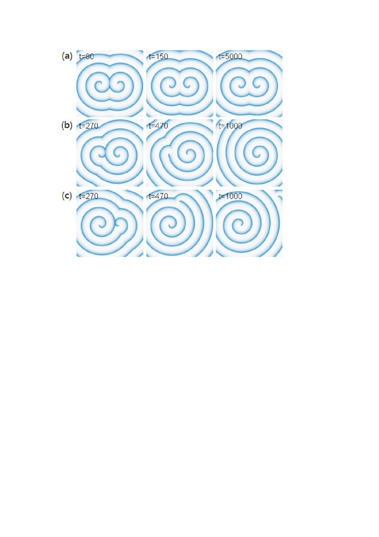
Figure 1: (color online). Chiral symmetry breaking and selection of a spiral pair under a CCW CPEF. (a) $E=0$, a spiral pair stably rotates. (b) $E=0.05$ and $\omega_{f}=0.87>\omega_{0}$, chiral symmetry breaking occurs, and chirality of the dominant spiral is CCW, the same as that of the CPEF. (c) similar to (b), but with $\omega_{f}=0.83<\omega_{0}$, the dominant spiral is CW, opposite to that of the CPEF. Numbers shown in each plot indicate the time. We show the $v$ variable in each snapshot. The system is composed of $1024\times 1024$ grid points.

In this section we investigate the behavior of a spiral pair under a CPEF. To this end, we first initiate a pair of two counter-rotating spiral waves as shown in Fig. 1(a); such pair is invariant under mirror symmetry. We note that dynamics of a spiral pair has been studied by many authors aranson ; villarreal_pre ; villarreal_prl ; schebesch ; aranson_prl96 . For instance, in the framework of CGLE, a spiral pair undergoes a symmetry breaking instability. Such kind of breaking has been further reported experimentally in the BZ system villarreal_pre ; brandtstadter and numerically in the three-component RD systems schebesch ; aranson_prl96 . In our case such kind of instability does not occur without the electric terms in Eqs. (1-2). Figure 1(b) shows a process of the chiral symmetry instability of the spiral pair after switching on the CCW CPEF with $E=0.05$ and $\omega_{f}=0.87$, slightly larger than the rotation frequency $\omega_{0}$ of a free spiral. In less than 36 rotations, chiral symmetry is clearly lost [refer to t=270 t.u. in Fig. 1(b)], and then the CCW spiral with the same chirality as the CPEF starts to dominate (refer to t=470 t.u.). Later, the CW spiral is pushed to the boundary and only the CCW spiral wave survives in the system (t=1000 t.u.). Note that in this case the external field selects a spiral with the same chirality as its own, which is consistent with the chiral selection controlled by chiral fields in other systems ecke_sci ; miglerprl ; nicolis_pnas ; ribo ; noorduin ; toyoda .

Figure 2: (color online). Chiral selection in a multiple-spiral state caused by a CCW CPEF. (a) $E=0.0$, stable multiple-spiral state. (b) $E=0.05$, $\omega_{f}=0.87$, CCW spiral waves dominate at $t=5000$ t.u.. (c) $E=0.05$, $\omega_{f}=0.83$, CW spiral waves dominate CCW at $t=3000$ t.u..The same system size and parameters as in Fig. 1 were used.

However, the opposite chirality (CW) spiral wave can also be selected without changing the chirality of the CPEF. This scenario is illustrated in Fig. 1(c) where we keep the same chirality for the CPEF as in Fig. 1(b), but lower the forcing frequency $\omega_{f}$ to $0.83<\omega_{0}$. In contrast to Fig. 1(b), we observe the CW spiral develops and the other one is reduced to a bare core. Thus, the spiral with the opposite chirality to the CPEF is eventually selected. This scenario is quite different from the previous studies on the chiral symmetry breaking caused by chiral fields, where reversal of the chiral field chirality seems necessary if one needs to select the opposite chiral entity. ecke_sci ; miglerprl ; nicolis_pnas ; ribo ; noorduin ; toyoda .

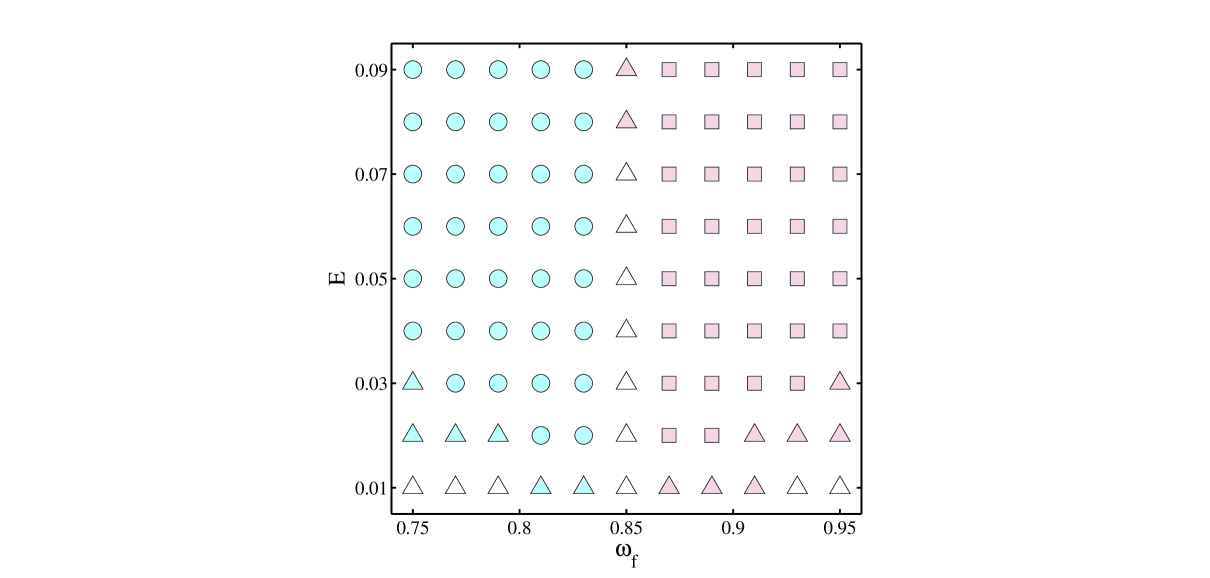
Figure 3: (color online). Phase diagram of chiral selection controlled by the CCW CPEF. Shaded circles and squares denote the CW and CCW dominant spiral waves, respectively; shaded triangles mean that the CCW and CW spiral still coexist but chiral symmetry breaking can be observed. Open triangle denotes the coexistence of the CCW and the CW spiral waves without obvious chiral symmetry breaking at the end of the simulation time $t_{tot}=1000$ t.u.. To compute this diagram, we use the same system size as in Fig. 1.

III.2 Chiral selection of multi-spiral states

The present findings also differ from the spontaneous symmetry breaking of spiral pairs found previously where chiral selection of the dominant spiral is unpredictable which is sensitive to the many factors such as the initial distance between the spiral corearanson ; villarreal_pre ; villarreal_prl ; schebesch ; aranson_prl96 ; brandtstadter . However, the forced chiral symmetry breaking caused by the CPEF presented in this work [both in Fig. 1(b) and (c)] is quite robust and almost insensitive to the initial orientation or inter-spiral distance. For example, the chiral symmetry breaking observed above is not only limited to a spiral pair and it can also occur in a state with multiple spiral waves, as illustrated in Fig. 2. Similar to the interaction of a spiral pair, we find CCW spiral waves would dominate CW spiral waves when we apply CCW CPEF with $\omega_{f}=0.87>\omega_{0}$ and CW spirals finally dominate CCW ones as we change the forcing frequency to $\omega_{f}=0.83<\omega_{0}$.

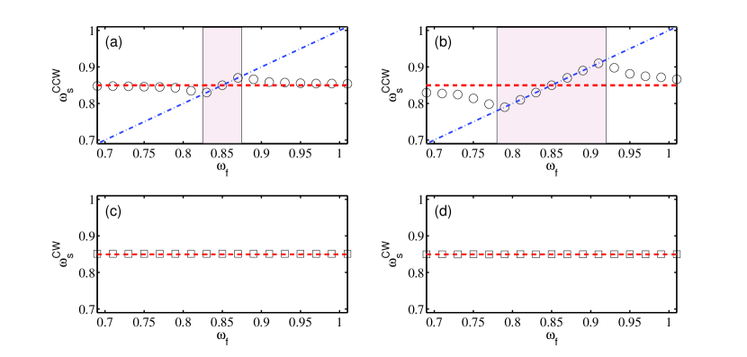
Figure 4: (color online). Spiral frequency response to the CCW CPEF. (a-b) The frequency of a CCW spiral wave as a function of the forcing frequency $\omega_{f}$ for $E=0.02$ and $E=0.05$, respectively. (c-d) The frequency of a CW spiral as a function of $\omega_{f}$ for $E=0.02$ and $E=0.05$, respectively. The red dashed lines represent $\omega_{0}=0.851$. In (a-b), the shaded region denotes the synchronized region and the blue dots lines mean $\omega_{s}=\omega_{f}$. To calculate the frequency (period), we use the system with $256\times 256$ grid points.

III.3 Phase diagram for chiral selection

A systematic study shows that such chiral symmetry breaking and pattern selection can be achieved in a broad parameter range. We summarize the results in the phase diagram of $E$ versus $\omega_{f}$ in Fig. 3. After a spiral pair is created ($t=40$ t.u.), the CPEF is switched on and the evolution is followed until the simulation was ended ($t=t_{e}=1040$ t.u.). Different final states are coded with different markers in Fig. 3. First, when no obvious chiral breaking is noticed, open triangles are drawn. This happened near resonance ($\omega_{f}\approx\omega_{0}$) and at the lower corners of the diagram where $|\omega_{f}-\omega_{0}|/E$ is large. Secondly, we drew shaded circles (squares) when a single dominant CW (CCW) spiral pattern survived. As in Fig. 1(a-b), these regions correspond to where $\omega_{f}$ is slightly smaller (bigger) than $\omega_{0}$. Third, between the fully selective and non-selective regions of the phase diagram, a border zone exists (colored triangles), where chiral symmetry was broken at $t=t_{e}$, without achieving a selection of single-chirality spiral waves.

III.4 Frequency response of spiral waves to a CPEF

The time-averaged spiral frequency $\omega_{s}$ is measured (refer to the section of the numerical method) and its dependence on the forcing frequency $\omega_{f}$ for two intensities $E$ is plotted in Fig. 4 (a-b) for the CCW spiral and Fig. 4(c-d) for the CW one. From these plots, we find that there is a chirality-dependent frequency response of spiral waves to the CPEF. Specifically, the CCW spiral with the same chirality as the CPEF, is able to keep the pace with the CPEF, which is particularly obvious if the frequency mismatch between $\omega_{f}$ and $\omega_{0}$, denoted by $\Delta\omega=\omega_{f}-\omega_{0}$, is small. Once this happens, $\omega^{CCW}_{s}$ would be altered to keep the same value as $\omega_{f}$ and frequency synchronization, also known as phase-locking, is observed. The synchronization region (color shaded) is extended as we increase the strength of the CPEF [compared Fig. 4(a) to 4(b)]. However, rotation frequency of the spiral waves with opposite chirality to the CPEF, seems to be hardly affected by the frequency and the intensity of the CPEF. The rotation frequency of CW spirals stays close to $\omega_{0}$, as seen from Figs. 4(c-d).

IV Mechanism for chiral selection and frequency synchronization

IV.1 Selection of spiral waves by frequency shift

The chirality-dependent frequency response to the CPEF is the underlying cause for the chiral selection observed in Figs. (1-3) as we explain below from the viewpoint of the wave competition. When we apply a CCW CPEF with the frequency that is quite close to but a little larger than $\omega_{0}$, i.e., $\omega_{f}>\omega_{0}$, from Fig. 4 we know the rotation frequency of the CCW spiral with the same chirality as the CPEF would be increased due to synchronization: i.e., $\omega^{CCW}_{s}=\omega_{f}$; while for the CW spiral, its frequency $\omega^{CW}_{s}$ seems not changed and thus $\omega^{CW}\approx\omega_{0}$. This causes a frequency shift between CCW and CW spiral waves when a spiral pair is affected by the CPEF. Due to the competition rule that in excitable media the faster one always win the slower one, we find at the end the CCW spiral dominates the CW one in Fig. 1(b). E.g. the faster source may push its wave tail closer to the other spiral’s core, which is eventually directly exposed to the spiral wave of the higher frequency. As a result the slower rotating wave will drift, and may be annihilated at the medium boundary. The scenario is also very similar if we apply the CPEF with $\omega_{f}<\omega_{0}$, e.g., see Fig. 1(c). This competition also explains the scenarios witnessed in Figs. (2-3).

When we apply $\omega_{f}$ that is almost equal to $\omega_{0}$, we will get $\omega^{CCW}_{s}\approx\omega^{CW}_{s}$, and under this situation, a spiral pair will still be stable as the case without the CPEF. If the frequency shift between spiral waves caused by the CPEF is extremely small, we need a much longer time to observe chiral symmetry breaking, which explains the narrow zone at $\omega_{f}\approx\omega_{0}$ in Fig. 3 where chiral symmetry was intact at the end of simulation time.

IV.2 Theoretical description of frequency synchronization using response function theory

In order to look into the nature and origin of the chirality-dependent frequency response, especially frequency synchronization, in further detail, we below derive a phase equation based on the based on the singular perturbation theory biktashev94 ; biktashevapre03 ; biktashevapre09 ; biktashevapre10 ; dxspiral ; dierckx2 ; keener86 ; henrypre02 ; mikhailov94 around an unperturbed spiral wave, employing critical adjoint eigenfunctions which are also known as response functions biktashev94 ; biktashevapre03 ; biktashevapre09 ; biktashevapre10 ; dxspiral ; dierckx2 . From this phase equation, we analytically find the conditions under which a spiral wave will synchronize with the CPEF, as we now proceed to show.

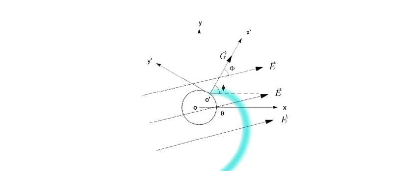
Figure 5: (color online). A scheme of defining references and angles for our derivation. $xoy$ is fixed in the lab reference, while $x^{\prime}o^{\prime}y^{\prime}$ co-rotates with the spiral at the instantaneous frequency $\omega$. $o^{\prime}x^{\prime}$ is chosen as parallel with the vector $\vec{G}=\vec{\nabla}u/||\vec{\nabla}u||$ at the spiral tip. For then, $\Phi=\phi(t)-\theta(t)$ where $\theta(t)=\theta_{0}+\omega_{f}t$ and $\phi(t)=\phi_{0}+\omega_{0}t+\tilde{\phi}(t)$ denote the rotation phases of the electric field and the spiral wave. The shaded region denotes the shape of the spiral wave.

We start our derivation of the phase-locking equation by rewriting Eqs.(1-2) in a matrix form,

$$\partial_{t}\textbf{u}=\hat{\textbf{D}}\triangle\textbf{u}+\textbf{F(u)}+\textbf{h},$$ (3)

where in our case $\textbf{u}=(u,v)^{T}$, $\textbf{F}=(\varepsilon^{-1}(u-u^{2}-(fv+\varphi)(u-q)/(u+q)),u-v)^{T}$ and $\textbf{h}=\vec{E}\cdot\hat{\textbf{M}}\vec{\nabla}\textbf{u}$ is assumed to be a small perturbation. Furthermore, $\hat{\textbf{D}}$ and $\hat{\textbf{M}}$ are constant diffusion and mobility matrices, given by

$$\hat{\textbf{D}} =\left(\begin{array}[]{cc}D_{u}&0\\ 0&D_{v}\end{array}\right), \hat{\textbf{M}} =\left(\begin{array}[]{cc}M_{u}&0\\ 0&M_{v}\end{array}\right).$$ (8)

Next, we introduce two frames of reference as shown in Fig. 5. The laboratory frame is denoted by $(x,y,t)$, while the spiral frame that co-rotates with the spiral wave at the instantaneous frequency $\omega$ is denoted by $(x^{\prime},y^{\prime},t^{\prime})$. To measure the spiral’s rotation phase, we introduce the reference vector $\vec{G}=\vec{\nabla}u/||\vec{\nabla}u||$ at the spiral tip. The phase $\phi$ is then the oriented angle between the $X$-direction and $\vec{G}$. We will choose the co-rotating frame such that $\vec{G}$ is aligned with the positive X’-axis at all times.

Furthermore, we denote by $\sigma$ the chirality of the spiral wave: $\sigma=+1$ for CCW and $\sigma=-1$ for CW rotation. (As before, we assume the rotation of the CPEF is always CCW, i.e., $\omega_{f}>0$.)

According to the response function theory used in Refs. biktashev94 ; biktashevapre03 ; biktashevapre09 ; biktashevapre10 ; dxspiral ; dierckx2 , a small perturbation h acts on a robust spiral pattern by causing a translational and rotational shift. In particular, the phase angle will evolve as $\phi(t)=\phi_{0}+\sigma\omega_{0}t+\tilde{\phi}(t)$ with phase correction $\tilde{\phi}(t)$. Hence, the instantaneous rotation frequency changes to $\dot{\phi}(t)=\sigma\omega_{0}+\tilde{\omega}(t)$ where $\tilde{\omega}(t)=\dot{\tilde{\phi}}(t)$ is a convolution of h with the so-called rotational response function dierckx2 , i.e.,

$$\tilde{\omega} = \int_{\mathbb{R}^{2}}{\textbf{W}^{(0)}(x^{\prime},y^{\prime})^{H}\textbf{h}(x^{\prime},y^{\prime},t^{\prime})dx^{\prime}dy^{\prime}.}$$ (9)

Here $(.)^{H}$ denotes Hermitian conjugation of a column vector of state-variables and $\textbf{W}^{(0)}$ is the rotational response function. Mathematically, it is the adjoint zero mode to the linearized operator associated to Eq. (3) keener86 ; biktashevapre09 ; dierckx2 . We use the normalization as in Ref. biktashevapre09 such that

$$\int_{\mathbb{R}^{2}}\textbf{W}^{(0)}(X,Y)^{H}\partial_{\Theta}\textbf{u}_{0}(X,Y)dXdY=-1,$$ (10)

to avoid the appearance of a minus sign in Eq. (9). Here, $\textbf{u}_{0}(X,Y)$ is the time-independent unperturbed spiral wave solution to Eq. (3) in the co-rotating frame with polar coordinate $\Theta$. For a given RD model with differentiable reaction kinetics, $\textbf{W}^{(0)}$ can be numerically computed, see e.g. Refs.henrypre02 ; biktashevapre09 . In the present case, the perturbation is the CPEF, i.e., $\textbf{h}=\vec{E}\cdot\hat{\textbf{M}}\vec{\nabla}\textbf{u}$, which can be expressed in the spiral frame ($x^{\prime}o^{\prime}y^{\prime}$) as

h $$= E^{x^{\prime}}\hat{\textbf{M}}\partial_{x^{\prime}}\textbf{u}+E^{y^{\prime}}\hat{\textbf{M}}\partial_{y^{\prime}}\textbf{u}=E^{x^{\prime}}\hat{\textbf{M}}\partial_{x^{\prime}}\textbf{u}_{0}+E^{y^{\prime}}\hat{\textbf{P}}\partial_{y^{\prime}}\textbf{u}_{0}+O(E^{2}).$$ (11)

Here $E^{x^{\prime}}$ ($E^{y^{\prime}}$) is the component of the electric field $\vec{E}$ along $x^{\prime}$ ($y^{\prime}$) and a first approximation is made, i.e., $\textbf{u}(x^{\prime},y^{\prime},t^{\prime})=\textbf{u}_{0}(x^{\prime},y^{\prime})+\tilde{\textbf{u}}(x^{\prime},y^{\prime},t^{\prime}),$ where $\tilde{\textbf{u}}$ is of the same order as $E$. Substituting Eq. (11) to Eq. (9), we have,

$$\tilde{\omega} = \dot{\tilde{\phi}}=E^{x^{\prime}}M_{x^{\prime}}^{0}+E^{y^{\prime}}M_{y^{\prime}}^{0}+O(E^{2}),$$ (12)

where $M_{x^{\prime}}^{0}$ and $M_{y^{\prime}}^{0}$ are time-independent constants given by the overlap integrals

$$M_{x^{\prime}}^{0}=\int_{\mathbb{R}^{2}}{\textbf{W}^{(0)}(x^{\prime},y^{\prime})^{H}\hat{\textbf{M}}\partial_{x^{\prime}}\textbf{u}_{0}(x^{\prime},y^{\prime})dx^{\prime}dy^{\prime}},M_{y^{\prime}}^{0}=\int_{\mathbb{R}^{2}}{\textbf{W}^{(0)}(x^{\prime},y^{\prime})^{H}\hat{\textbf{M}}\partial_{y^{\prime}}\textbf{u}_{0}(x^{\prime},y^{\prime})dx^{\prime}dy^{\prime}}.$$ (13)

Let us now denote the experimentally accessible angle of $\vec{G}$ relative to the electric field as $\Phi(t)=\phi(t)-\theta(t)$, which yields $E^{x^{\prime}}=E\cos\Phi$ and $E^{y^{\prime}}=-E\sin\Phi$. If we further define $M_{x^{\prime}}^{0}=A\cos\alpha$ and $M_{y^{\prime}}^{0}=A\sin\alpha$ such that

$$A =\sqrt{(M_{x^{\prime}}^{0})^{2}+(M_{y^{\prime}}^{0})^{2}}, \tan\alpha =M_{y^{\prime}}^{0}/M_{x^{\prime}}^{0},$$ (14)

Eq. (12) can be written as

$$\dot{\tilde{\omega}}=\dot{\tilde{\phi}}=EA\cos(\Phi+\alpha)+O(E^{2}).$$ (15)

Recalling that $\Phi(t)=\phi(t)-\theta(t)$, we note that $\dot{\Phi}=(\sigma\omega_{0}-\omega_{f})+\dot{\tilde{\phi}}$, which finally produces the phase equation, up to linear order in the field intensity $E$:

$$\dot{\Phi}(t)=-\Delta\omega+EA\cos(\Phi+\alpha),$$ (16)

where $\Delta\omega=\omega_{f}-\sigma\omega_{0}$.

Interestingly, we note that Eq. (16) has the same form as with phase synchronization of oscillators driven by a small periodic force kuramoto ; pikovsky where it is often called the Adler equation adler . This equation is served to study phase-locking phenomena in diverse natural or engineered systemsadler ; kuramoto . Furthermore, the coefficients $A$ and $\alpha$ can be found from numerical computation, as we will proceed to show.

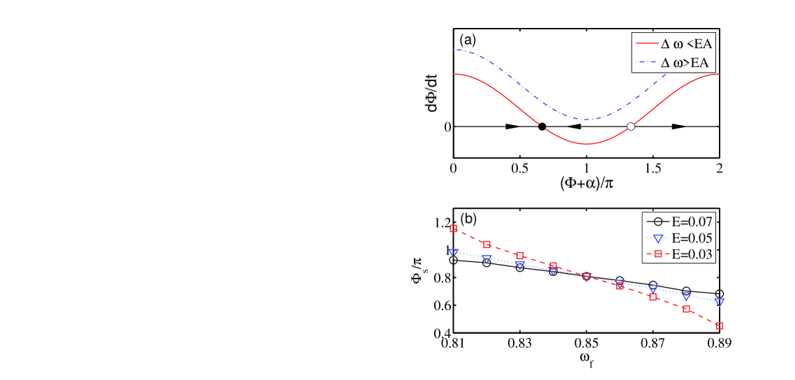
Figure 6: (color online). (a) Plot of $\dot{\Phi}$ versus $(\Phi+\alpha)$. The solid black dot represents the stable solution (fixed point) while the open circle denotes the unstable one. Arrows denote the flow direction. (b) Dependence of numerically measured $\Phi_{s}$ on $\omega_{f}$ for three different intensities of the electric field.

Let us first, however, discuss how frequency synchronization follows from Eq. (16). Since $|\cos(x)|\leq 1$ for all real-valued arguments $x$, in the case of the same rotation between spiral waves and the CPEF the one-dimensional dynamical system Eq. (16) possesses two equilibrium points $\Phi_{\pm}=-\alpha\pm\arccos\left(\frac{\Delta\omega}{EA}\right)$ whenever $|\omega_{0}-\omega_{f}|<EA$. From Fig. 6(a), it is observed that only the equilibrium point which has $0<\Phi+\alpha<\pi$ is stable; we will denote it as

$$\Phi_{s}=-\alpha+\arccos\left(\frac{\Delta\omega}{EA}\right).$$ (17)

Hence, a unique phase-locked spiral state exists as long as

$$E>E_{*}=\frac{\left|\omega_{0}-\omega_{f}\right|}{A}.$$ (18)

Such phase-locking region is known as an Arnold tongue; for the current system and order of calculation in $E$, it has a triangular shape.

If the spiral wave and the CPEF rotate in an opposite way, the phase equation can be written explicitly as $\dot{\Phi}=-(\omega_{0}+\omega_{f})+EA\cos(\Phi+\alpha)$. Since we work in the regime of $EA<<(\omega_{0}+\omega_{f})$, we expect no synchronization in this case, which is consistent with the observation in Fig. 4(c-d).

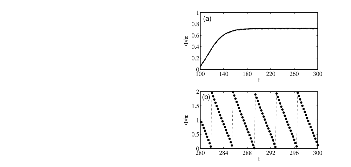
Figure 7: (a) $\Phi$ changes as time for $E=0.05$ and $\omega_{f}=0.87$ showing the phase locking for large $t$. Both the spiral and the CPEF are CCW. (b) Same as (a) but for the opposite chirality, e.g., CW spiral and CCW CPEF.

IV.3 Quantitative results using response functions

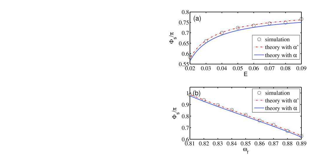
Figure 8: (color online). A comparison of theory with numerical simulations. (a) $\Phi_{s}$ as a function of $E$ for $\omega_{f}=0.87$; (b) $\Phi_{s}$ as a function of $\omega_{f}$ for $E=0.05$. Theoretical predictions from Eq. (17) with $\alpha^{\prime}=-0.9722$ [calculated from Eq. (17) and Fig. 6(b)] and $\alpha=-0.9334$ (calculated from the response functions) are used. The same system size as in Fig. 4 is used to compute these plots.

Finally, we will quantitatively compare the theory and numerical experiments for the value of the phase-locked angle and the width of the Arnold tongue. These quantities only depend on the parameters $A$ and $\alpha$, which are fully determined by the parameters of the RD system without the electric field. They can be directly calculated with response functions by using the freely available software dxspiral biktashevapre09 ; biktashevapre10 ; dxspiral , to which we added reaction kinetics for the Oregonator model. With the parameters used in our paper and a polar grid of radius $R=10$ with $N_{r}=240,N_{\theta}=256$, we find $A=1.505$. In the frame where $x^{\prime}$ is aligned with $\vec{G}$, we find $M^{\theta}_{x^{\prime}}=0.8955$, $M^{\theta}_{y^{\prime}}=-1.2094$, such that $\alpha=-0.9334=-53.5^{\circ}$.

To compare our theory and simulations, we first note that at resonance ($\Delta\omega=0$), the relation Eq. (17) predicts that the phase-locked angle found between $\vec{E}$, $\vec{G}$ should equal $\Phi_{s}(\Delta\omega=0)=-\alpha+\pi/2.$ In our numerical experiment, $\Phi_{s}(\Delta\omega=0)$ was measured to be $145.7^{\circ}$, as seen in Fig. 6(b) where we plot $\Phi_{s}$ as function of $\omega_{f}$, yielding $\alpha^{\prime}=-0.9722=-55.70^{\circ}$. (We here use $\alpha^{\prime}$ to distinguish from the value of $\alpha$ that is directly calculated from the response functions.) This value $\alpha^{\prime}$ is closely matched by our response function calculation above (i.e., $\alpha$), with an error about $2.2^{\circ}$.

Figure 7 shows the typical evolution for $\Phi$, the spiral phase relative to the electric field, in the case of phase-locking [Fig. 7(a)] or no phase-locking [Fig. 7(b)]. Panel 7(a) shows the change of $\Phi$ as time elapses for the CCW spiral in the presence of the CCW CPEF with $E=0.05$ and $\omega_{f}=0.87$. One observes that $\Phi$ eventually reaches a constant, indicating frequency synchronization (i.e., phase-locking). In Fig. 7(b) with the same parameters but with CW spiral waves, however, $\Phi$ changes periodically with period close to $2\pi/(\omega_{f}+\omega_{0})$. The system behavior in both panels is consistent with Eq. (16).

In the synchronization case, $\Phi_{s}$ is determined by Eq. (17), implying that both $\Delta\omega$ and $E$ affect the phase-locked angle $\Phi_{s}$. In Fig. 8(a), we predict the dependence of $\Phi_{s}$ on $E$ given $\omega_{f}=0.87$ (i.e., $\Delta\omega=0.02$) using Eq. (17) with $A$ and above mentioned values of $\alpha$ (and $\alpha^{\prime}$). One observes that the simulation results agree well with the theoretical prediction from Eq. (17). Similarly, the graph in Fig. 8(b) of $\Phi_{s}$ as a function of $\omega_{f}$ given $E=0.05$ also shows a nice correspondence between simulations and theory. Note that a linear dependency of $\Phi_{s}$ on $\omega_{f}$ is found since $\arccos(x)\approx\pi/2-x$ in the frequency synchronization regime shown here.

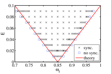
Figure 9: (color online). Arnold synchronized tongue. The crosses and square denote the numerical simulations where synchronization and unsynchronization behaviors are observed; the red line shows the boundary derived from Eq. (16) with $A=1.505$ (without free parameters). To compute this plot, we use the same system size as in Fig. 4.

To give a complete comparison between these predictions and numerical results, we present in Fig. 9 the Arnold tongue for synchronization in the parameter space of $\omega_{f}$ and $E$. In this figure, crosses denote the numerical results of the synchronization. For each value of $E$ shown, we started simulations in the synchronization zone and increased or decreased $\omega_{f}$ until synchronization could no longer be established. The couples ($E,\omega_{f}$) where synchronization failed are represented by the blue squares in Fig. 9. For comparison, the red line denotes the synchronization boundary that is derived from Eq. (18). We find that a good agreement is achieved for the small $E$. Note that, for $E>0.05$ deviations are visible which may be captured by extending our linear theory to high orders in $E$ in the future.

Finally, it is noted that synchronous mechanism plays an important role in the chiral selection shown in Figs. (1-2), however, such kind of chiral symmetry breaking is not only limited to the synchronous region as seen by comparing the Arnold tongue (Fig. 9) with the phase diagram (Fig. 3). This is because even in the not fully synchronized region, the CPEF can also cause a chirality-dependent frequency response as illustrated in Fig. 4 (outside the shaded region). For example, in the unsynchronized regime but still close to synchronous regime, the spiral frequency would be still larger (smaller) than $\omega_{0}$ if we apply the CPEF with $\omega_{f}$ larger (smaller) than $\omega_{0}$. Therefore even in the non-synchronous region, we could also observe chiral symmetry breaking and pattern selection.

V Discussion

By studying the instability of spiral pairs in the Oregonator model subject to the CPEF, we demonstrated and quantitatively analyzed the chiral selection of spiral pairs controlled by a chiral electric field. Our results are different from the previous findings. On one hand, prior to our work, most of works showed that the chirality of the dominant pattern seemed fully determined by that of the applied field, however, our work showed another possibility in chemical media that the dominant spiral pattern could be the same as or opposite to the chirality of the CPEF. On the other hand, in previous work, chirality-dependent frequency response, especially frequency synchronization between spiral waves and the applied CPEF was only discussed in the phenomenological level and the dynamical mechanism was unclear. In the present work, based on the response function theory, we found the coupling of spiral waves and the applied CPEF can be transformed to a phase equation that governs the evolution of the angle of spiral orientation relative to the electrical field. From this equation, we could make several quantitative predications that were validated by our numerical simulations. It is worth noting that our findings were quite robust and insensitive to the specific models. For example, we also checked the main results in Barkley’s model barkley91 and found similar results. From this point of view, our present work allows us to understand better about the interaction between spiral waves and the CPEF and provides a solid basis for chirality control in excitable media.

We would like to point out that the proposed theory for frequency synchronization is applicable for the rigidly rotating spiral waves only. However, previous work showed that such CPEF induced frequency synchronization or phase-locking also occurs for the meandering spiral waves chenjcp2 . It would be important to extend our theory in future to describe such phase locking phenomenon for the meandering case.

Finally, the findings present in this work can be directly tested in chemical experiments, since the CPEF has been recently realized in the BZ system jipre . Compared to the spiral turbulence state jipre , we believe that it is easier to observe chiral symmetry breaking and pattern selection by considering a stable spiral pair under the CPEF. For, to observe chiral symmetry breaking in the spiral turbulence state, in addition to consider the wave competition between spiral waves, we also need to consider the issue of stabilization of the unstable spirals. This would take longer time and require stronger intensity of the CPEF. The latter factor is quite important in the implementation of the CPEF in the laboratory because the stronger intensity of the CPEF could cause increased heat production which leads to some serious problems (e.g., higher or uncontrollable excitability) for the experimental set-upjipre .

VI Conclusion

In summary, we have investigated chiral symmetry breaking and pattern selection in RD systems (Oregonator model) coupled to the CPEF. We have shown that the chirality of dominant pattern can be well controlled by the applied electric field in the synchronous (or unsynchronous) regime. More interestingly, we showed that we can select an opposite chiral pattern by tuning the forcing frequency instead of changing the chirality of the CPEF. We attribute this scenario to the chirality-dependent frequency response to the CPEF, which can be quantitatively described by the Adler equation that we have originally derived using response function theory. Our predictions agree well with the numerical results. Finally, considering the recent realization of the CPEF in the BZ system and that our results are robust throughout numerical simulations, we believe that our findings presented here are highly likely to be observed in the laboratory.

References

- (1) G. H. Wagniere, On Chirality and the Universal Asymmetry (Wiley-VCH, Zurich, Weinheim, 2007).
- (2) A. T. Winfree, Science 175, 634 (1972).
- (3) Q. Ouyang and J. M. Flesselles, Nature (London) 379, 143 (1996).
- (4) V. K. Vanag and I. R. Epstein, Science 294, 835 (2001).
- (5) S. Jakubith, H. H. Rotermund, W. Engel, A. von Oertzen, and G. Ertl, Phys. Rev. Lett. 65, 3013 (1990); S. Nettesheim, A. von Oertzen, H. H. Rotermund, and G. Ertl, J. Chem. Phys. 98, 9977 (1993).
- (6) T. Frisch, S. Rica, P. Coullet, and J. M. Gilli, Phys. Rev. Lett. 72, 1471 (1994).
- (7) K. J. Lee, E. C. Cox, and R. E. Goldstein, Phys. Rev. Lett. 76, 1174 (1996); S. Sawai, P. A. Thomason, and E. C. Cox, Nature (London) 433, 323 (2005).
- (8) Y. Yu et al., Proc. Natl. Acad. Sci. U.S.A. 109, 2585 (2012).
- (9) J. M. Davidenko, A. V. Pertsov, R. Salomonsz, W. Baxter, and J. Jalife, Nature (London) 355, 349 (1992).
- (10) J. Schütze, O. Steinbock, and S. C. Müller, Nature (London) 356, 45 (1992); O. Steinbock, J. Schütze, and S. C. Müller, Phys. Rev. Lett. 68, 248 (1992).
- (11) K. I. Agladze and P. De Kepper, J. Phys. Chem. 96, 5239 (1992).
- (12) V. Krinsky, E. Hamm, and V. Voignier, Phys. Rev. Lett. 76, 3854 (1996).
- (13) A. P. Muñuzuri, M. Gómez-Gesteira, V. Pérez-Muñuzuri, V. I. Krinsky, and V. Pérez-Villar, Phys. Rev. E 50, 4258 (1994).
- (14) J. J. Taboada, A. P. Muñuzuri, V. Pérez-Muñuzuri, M. Gómez-Gesteira, and V. Pérez-Villar, Chaos 4, 519 (1994).
- (15) B. Schmidt and S. C. Müller, Phys. Rev. E 55, 4390 (1997).
- (16) O. Steinbock, V. Zykov, and S. C. Müller, Nature 366, 322 (1993); V. S. Zykov, O. Steinbock, and S. C. Müller, Chaos 4, 509 (1994).
- (17) M. Braune, A. Schrader, and H. Engle, Chem. Phys. Lett. 222, 358 (1994).
- (18) R. M. Mantel and D. Barkley, Phys. Rev. E 54, 4791 (1996).
- (19) A. L. Lin, M. Bertram, K. Martinez, and H. L. Swinney, A. Ardelea, and G. F. Carey Phys. Rev. Lett. 84, 4240 (2000); A. L. Lin, A. Hagberg, E. Meron, and H. L. Swinney, Phys. Rev. E 69, 066217 (2004).
- (20) H. Zhang, Z. Cao, N. J. Wu, H. P. Ying, and G. Hu, Phys. Rev. Lett. 94, 188301 (2005).
- (21) A. P. Muñuzuri, C. Innocenti, J.-M. Flesselles, J.-M. Gilli, K. I. Agladze, and V. I. Krinsky, Phys. Rev. E 50, R667 (1994).
- (22) A. V. Panfilov, R. H. Keldermann, and M. P. Nash, Proc. Natl. Acad. Sci. U.S.A. 104,7922 (2007).
- (23) L. D. Weise and A. V. Panfilov, Phys. Rev. Lett. 108, 228104 (2012).
- (24) X. Zou, H. Levine, and D. A. Kessler, Phys. Rev. E 47, R800 (1993).
- (25) V. N. Biktashev, D. Barkley, and I. V. Biktasheva, Phys. Rev. Lett. 104, 058302 (2010).
- (26) B. W. Li, H. Zhang, H. P. Ying, and G. Hu, Phys. Rev. E 79, 026220 (2009); B. W. Li, H. Zhang, H. P. Ying, W. Q. Chen, and G. Hu, Phys. Rev. E 77, 056207 (2008); T. C. Li and B. W. Li, Chaos 23 , 033130 (2013).
- (27) S. Alonso, K. John, and M. Bär, J. Chem. Phys. 134, 094117 (2011); S. Alonso and M. Bär, Phys. Rev. Lett. 110, 158101 (2013).
- (28) H. Dierckx, E. Brisard, H. Verschelde, and A. V. Panfilov, Phys. Rev. E 88, 012908 (2013).
- (29) A. Defauw, P. Dawyndt, and A. V. Panfilov, Phys. Rev. E 88, 062703 (2013).
- (30) G. Nicolis and I. Prigogine, Proc. Natl. Acad. Sci. U.S.A. 78, 659 (1981).
- (31) K. B. Migler and R. B. Meryer, Physica D 71, 412 (1994).
- (32) R. E. Ecke, Y. Hu, R. Mainieri, and G. Ahlers, Science 269, 1704 (1995).
- (33) K. Nam, E. Ott, M. Gabbay, and P. N. Guzdar, Physica D, 118, 69 (1998).
- (34) J. X. Chen, H. Zhang, and Y. Q. Li, J. Chem. Phys. 124, 014505 (2006).
- (35) L. Ji, Y. Zhou, Q. Li, C. Qiao, and Q. Ouyang, Phys. Rev. E 88, 042919 (2013).
- (36) J. X. Chen, H. Zhang, and Y. Q. Li, J. Chem. Phys. 130, 124510 (2009).
- (37) M. C. Cai, J. T. Pan, and H. Zhang, Phys. Rev. E 86, 016208 (2012).
- (38) B. W. Li, L. Y. Deng, and H. Zhang, Phys. Rev. E 87, 042905 (2013).
- (39) S. P. Carmichael and M. S. Shella, J. Chem. Phys. 139, 164705 (2013).
- (40) F. Ricci, F. H. Stillinger, and P. G. Debenedetti, J. Chem. Phys. 139, 174503 (2013).
- (41) J. M. Ribo, J. Crusats, F. Sagués, J. Claret, and R. Rubires, Science 292, 2063 (2001).
- (42) W. L. Noorduin et al., Nature Chem. 1, 729 (2009).
- (43) K. Toyoda, K. Miyamoto, N. Aoki, R. Morita, T. Omatsu. Nano Lett. 12, 3645 (2012).
- (44) S. Zykov, V. S. Zykov, and V. Davydov, EPL 73, 335 (2006).
- (45) I. Aranson, L. Kramer, and A. Weber, Physica D 53, 376 (1991); Phys. Rev. E. 48, R9 (1993).
- (46) M. Ruiz-Villarreal, M. Gómez-Gesteira, C. Souto, A. P. Muñuzuri, and V. Pérez-Villar, Phys. Rev. E 54, 2999 (1996).
- (47) M. Ruiz-Villarreal, M. Gómez-Gesteira, and V. Pérez-Villar, Phys. Rev. Lett. 78, 779 (1997).
- (48) I. Aranson, H. Levine, and L. Tsimring, Phys. Rev. Lett. 76, 1170 (1996)
- (49) I. Schebesch and H. Engel, Phys. Rev. E 60, 6429 (1999).
- (50) H. Brandtstädter, M. Braune, I. Schebesch, and H. Engel, Phys. Rev. E 323, 145 (2000).
- (51) I. V. Biktasheva, D. Barkley, V. N. Biktashev, G.V. Bordyugov, and A. J. Foulkes, Phys. Rev. E, 79, 056702 (2009).
- (52) I. V. Biktasheva, D. Barkley, V. N. Biktashev, and A. J. Foulkes, Phys. Rev. E 81, 066202 (2010).
- (53) D. Barkley, V. N. Biktashev, I. V. Biktasheva, G. V. Bordyugov, and A. J. Foulkes, “DXSPIRAL: code for studying spiral waves on a disk,” [http://cgi.csc.liv.ac.uk/~ivb/SOFTware/DXSpiral.html] (2008–2010), version 1.0.
- (54) I. V. Biktasheva and V. N. Biktashev, Phys. Rev. E 67, 026221 (2003).
- (55) J. P. Keener, SIAM J. Appl. Math. 46, 1039 (1986).
- (56) A. S. Mikhailov, V. A. Davydov, and V. S. Zykov, Physica D 70, 1 (1994).
- (57) H. Henry and V. Hakim, Phys. Rev. E 65, 046235 (2002).
- (58) V. N. Biktashev, A. V. Holden, and H. Zhang, Phil. Trans. R. Soc. London A 347, 611 (1994).
- (59) H. Dierckx and H. Verschelde, Phys. Rev. E 88, 062907 (2013).
- (60) Y. Kuramoto, Chemical Oscillations, Waves and Turbulence, (Springer,Berlin, 1984).
- (61) A. S. Pikovsky, M. Rosenblum, and J. Kurths, Synchronization: A Universal Concept in Nonlinear Sciences (Cambridge University Press, Cambridge, UK, 2001).
- (62) R. Adler, Proceedings of the IRE 34, 351 (1946).
- (63) D. Barkley, Physica D 49, 61 (1991).