Automated Fixing of
Programs with Contracts

Abstract

This paper describes AutoFix, an automatic debugging technique that can fix faults in general-purpose software. To provide high-quality fix suggestions and to enable automation of the whole debugging process, AutoFix relies on the presence of simple specification elements in the form of contracts (such as pre- and postconditions). Using contracts enhances the precision of dynamic analysis techniques for fault detection and localization, and for validating fixes. The only required user input to the AutoFix supporting tool is then a faulty program annotated with contracts; the tool produces a collection of validated fixes for the fault ranked according to an estimate of their suitability.

In an extensive experimental evaluation, we applied AutoFix to over 200 faults in four code bases of different maturity and quality (of implementation and of contracts). AutoFix successfully fixed 42% of the faults, producing, in the majority of cases, corrections of quality comparable to those competent programmers would write; the used computational resources were modest, with an average time per fix below 20 minutes on commodity hardware. These figures compare favorably to the state of the art in automated program fixing, and demonstrate that the AutoFix approach is successfully applicable to reduce the debugging burden in real-world scenarios.

1 Introduction

Theprogrammer’s ever recommencing fight against errors involves two tasks: finding faults; and correcting them. Both are in dire need of at least partial automation.

Techniques to detect errors automatically are becoming increasingly available and slowly making their way into industrial practice [14, 34, 77]. In contrast, automating the whole debugging process—in particular, the synthesis of suitable fixes—is still a challenging problem, and only recently have usable techniques (reviewed in Section 6) started to appear.

AutoFix, described in this paper, is a technique and supporting tool that can generate corrections for faults of general-purpose software completely automatically. AutoFix targets programs annotated with contracts—simple specification elements in the form of preconditions, postconditions, and class invariants. Contracts provide a specification of correct behavior that can be used not only to detect faults automatically [61] but also to suggest corrections. The current implementation of AutoFix is integrated in the open-source Eiffel Verification Environment [33]—the research branch of the EiffelStudio IDE—and works on programs written in Eiffel; its concepts and techniques are, however, applicable to any programming language supporting some form of annotations (such as JML for Java or the .NET CodeContracts libraries).

AutoFix combines various program analysis techniques—such as dynamic invariant inference, simple static analysis, and fault localization—and produces a collection of suggested fixes, ranked according to a heuristic measurement of relevance. The dynamic analysis for each fault is driven by a set of test cases that exercise the routine (method) where the fault occurs. While the AutoFix techniques are independent of how these test cases have been obtained, all our experiments so far have relied on the AutoTest random-testing framework to generate the test cases, using the contracts as oracles. This makes for a completely automatic debugging process that goes from detecting a fault to suggesting a patch for it. The only user input is a program annotated with the same contracts that programmers using a contract-equipped language normally write [80, 32].

In previous work, we presented the basic algorithms behind AutoFix and demonstrated them on some preliminary examples [91, 76]. The present paper discusses the latest AutoFix implementation, which combines and integrates the previous approaches to improve the flexibility and generality of the overall fixing technique. The paper also includes, in Section 5, an extensive experimental evaluation that applied AutoFix to over 200 faults in four code bases, including both open-source software developed by professionals and student projects of various quality. AutoFix successfully fixed 86 (or 42%) of the faults; inspection shows that 51 of these fixes are genuine corrections of quality comparable to those competent programmers would write. The other 35 fixes are not as satisfactory—because they may change the intended program behavior—but are still useful patches that pass all available regression tests; hence, they avoid program failure and can be used as suggestions for further debugging. AutoFix required only limited computational resources to produce the fixes, with an average time per fix below 20 minutes on commodity hardware (about half of the time is used to generate the test cases that expose the fault). These results provide strong evidence that AutoFix is a promising technique that can correct many faults found in real programs completely automatically, often with high reliability and modest computational resources.

In the rest of the paper, Section 2 gives an overview of AutoFix from a user’s perspective, presenting a fault fixed automatically; the fault is included in the evaluation (Section 5) and is used as running example. Section 3 introduces some concepts and notation repeatedly used in the rest of the paper, such as the semantics of contracts and the program expressions manipulated by AutoFix. Section 4 presents the AutoFix algorithm in detail through its successive stages: program state abstraction, fault localization, synthesis of fix actions, generation of candidate fixes, validation of candidates, and ranking heuristics. Section 5 discusses the experimental evaluation, including a detailed statistical analysis of numerous important measures. Section 6 presents related work and compares it with our contribution. Finally, Section 7 includes a summary and concluding remarks.

2 AutoFix in action

We begin with a concise demonstration of how AutoFix, as seen from a user’s perspective, fixes faults completely automatically.

2.1 Moving items in sorted sets

Class TWO_WAY_SORTED_SET is the standard Eiffel implementation of sets using a doubly-linked list. Figure 2 outlines features (members) of the class, some annotated with their pre- (require) and postconditions (ensure). As pictured in Figure 1, the integer attribute index is an internal cursor useful to navigate the content of the set: the set elements occupy positions 1 to count (another integer attribute, storing the total number of elements in the set), whereas the indexes 0 and count + 1 correspond to the positions before the first element and after the last. before and after are also Boolean argumentless queries (member functions) that return True when the cursor is in the corresponding boundary positions.

Figure 1: A doubly-linked list implementing TWO_WAY_SORTED_SET. The cursor index is on position 2. The elements are stored in positions 1 to 4, whereas positions 0 (before) and 5 (after) mark the list’s boundaries. count denotes the number of stored elements (i.e., four).

⬇

1 index: INTEGER – Position of internal cursor.

2

3 count: INTEGER – Number of elements in the set.

4

5 before: BOOLEAN – Is index = 0 ?

6 do Result := (index = 0) end

7

8 after: BOOLEAN – Is index = count + 1 ?

9

10 off: BOOLEAN – Is cursor before or after ?

11

12 item: G – Item at current cursor position.

13 require not off

14

15 forth – Move cursor forward by one.

16 require not after

17 ensure index = old index + 1

18

19 has (v: G): BOOLEAN – Does the set contain v ?

20 ensure Result implies count $\neq$  0

21

22 go_i_th (i: INTEGER) – Move cursor to position i.

23 require 0 $\!\leq$ i $\!\leq$ count + 1

24

25 put_left (v: G) – Insert v to the left of cursor.

26 require not before

27

28 move_item (v : G) – Move v to the left of cursor.

29 require

30 v $\neq$ Void

31 has (v)

32 local idx: INTEGER ; found: BOOLEAN

33 do

34 idx := index

35 from start until found or after loop

36 found := (v = item)

37 if not found then forth end

38 end

39 check found and not after end

40 remove

41 go_i_th (idx)

42 put_left (v)

43 end

Figure 2: Some features of class TWO_WAY_SORTED_SET.

Figure 2 also shows the complete implementation of routine move_item, which moves an element v (passed as argument) from its current (unique) position in the set to the immediate left of the internal cursor index. For example, if the list contains $\langle a,b,c,d\rangle$ and index is 2 upon invocation (as in Figure 1), move_item (d) changes the list to $\langle a,d,b,c\rangle$. move_item’s precondition requires that the actual argument v be a valid reference (not Void, that is not null) to an element already stored in the set (has(v)). After saving the cursor position as the local variable idx, the loop in lines 35–38 performs a linear search for the element v using the internal cursor: when the loop terminates, index denotes v’s position in the set. The three routine calls on lines 40–42 complete the work: remove takes v out of the set; go_i_th restores index to its original value saved in idx; put_left puts v back in the set to the left of the position index.

2.2 An error in move_item

Running AutoTest on class TWO_WAY_SORTED_SET for only a few minutes exposes, completely automatically, an error in the implementation of move_item.

The error is due to the property that calling remove decrements the count of elements in the set by one. AutoTest produces a test that calls move_item when index equals count + 1; after v is removed, this value is not a valid position because it exceeds the new value of count by two, while a valid cursor ranges between 0 and count + 1. The test violates go_i_th’s precondition (line 23), which enforces the consistency constraint on index, when move_item calls it on line 41.

This fault is quite subtle, and the failing test represents only a special case of a more general faulty behavior that occurs whenever v appears in the set in a position to the left of the initial value of index: even if index $\!\leq$ count initially, put_left will insert v in the wrong position as a result of remove decrementing count—which indirectly shifts the index of every element after index to the left by one. For example, if index is 3 initially, calling move_item (d) on $\langle a,d,b,c\rangle$ changes the set to $\langle a,b,d,c\rangle$, but the correct behavior is leaving it unchanged. Such additional inputs leading to erroneous behavior go undetected by AutoTest because the developers of TWO_WAY_SORTED_SET provided an incomplete postcondition; the class lacks a query to characterize the fault condition in general terms.

2.3 Automatic correction of the error in move_item

AutoFix collects the test cases generated by AutoTest that exercise routine move_item. Based on them, and on other information gathered by dynamic and static analysis, it produces, after running only a few minutes on commodity hardware without any user input, up to 10 suggestions of fixes for the error discussed. The suggestions include only valid fixes: fixes that pass all available tests targeting move_item. Among them, we find the “proper” fix in Figure 3, which completely corrects the error in a way that makes us confident enough to deploy it in the program.

⬇

43 if idx $>$ index then

44 idx := idx - 1

45 end

Figure 3: Correction of the error in move_item automatically generated by AutoFix.

The correction consists of inserting the lines 43–45 in Figure 3 before the call to go_i_th on line 41 in Figure 2. The condition idx $>$ index holds precisely when v was initially in a position to the left of index ; in this case, we must decrement idx by one to accommodate the decreased value of count after the call to remove. This fix completely corrects the error beyond the specific case reported by AutoTest, even though move_item has no postcondition that formalizes its intended behavior.

3 Preliminaries: contracts, tests, and predicates

To identify faults, distinguish between correct and faulty input, and abstract the state of objects at runtime, AutoFix relies on basic concepts which will now be summarized.

3.1 Contracts and correctness

AutoFix works on Eiffel classes equipped with contracts [60]. Contracts define the specification of a class and consist of assertions: preconditions (require), postconditions (ensure), intermediate assertions (check), and class invariants (translated for simplicity of presentation into additional pre- and postconditions in the examples of this paper). Each assertion consists of one or more clauses, implicitly conjoined and usually displayed on different lines; for example, move_item’s precondition has two clauses: v $\neq$ Void on line 30 and has(v) on line 31.

Contracts provide a criterion to determine the correctness of a routine: every execution of a routine starting in a state satisfying the precondition (and the class invariant) must terminate in a state satisfying the postcondition (and the class invariant); every intermediate assertion must hold in any execution that reaches it; every call to another routine must occur in a state satisfying the callee’s precondition. Whenever one of these conditions is violated, we have a fault, uniquely identified by a location in the routine where the violation occurred and by the specific contract clause that is violated. For example, the fault discussed in Section 2 occurs on line 42 in routine move_item and violates the single precondition clause of put_left.

3.2 Tests and correctness

In this work, a test case $t$ is a sequence of object creations and routine invocations on the objects; if $r$ is the last routine called in $t$, we say that $t$ is a test case for $r$. A test case is passing if it terminates without violating any contract and failing otherwise.

Every session of automated program fixing takes as input a set $T$ of test cases, partitioned into sets $P$ (passing) and $F$ (failing). Each session targets a single specific fault—identified by some failing location $f$ in some routine $r$ and by a violated contract clause $c$. When we want to make the targeted fault explicit, we write $T_{r}$, $P_{r}$, and $F_{r}^{f,c}$. For example, ${{F^{{\ref{ln:putleft},\text{\mbox{\leavevmode\lstinline{{\lst@@@set@language\lst@@@set@numbers\lst@@@set@frame\lst@@@set@rulecolor\lst@@@set@numbers\lst@@@set@language{\@listingGroup{ltx_lst_keyword}{\color[rgb]{0,0,0}not}}{\@listingGroup{ltx_lst_space}{ }}{\@listingGroup{ltx_lst_identifier}{\color[rgb]{0,0,0}before}}}}}}}}}_{{\text{\mbox{\leavevmode\lstinline{{\lst@@@set@language\lst@@@set@numbers\lst@@@set@frame\lst@@@set@rulecolor\lst@@@set@numbers\lst@@@set@language{\@listingGroup{ltx_lst_identifier}{\color[rgb]{0,0,0}move\textunderscore item}}}}}}}}}$ denotes a set of test cases all violating put_left’s precondition at line 42 in move_item.

The fixing algorithm described in Section 4 is independent of whether the test cases $T$ are generated automatically or written manually. The experiments discussed in Section 5 all use the random testing framework AutoTest [61] developed in our previous work. Relying on AutoTest makes the whole process, from fault detection to fixing, completely automatic; our experiments show that even short AutoTest sessions are sufficient to produce suitable test cases that AutoFix can use for generating good-quality fixes.

3.3 Expressions and predicates

AutoFix understands the causes of faults and builds fixes by constructing and analyzing a number of abstractions of the program states. Such abstractions are based on Boolean predicates that AutoFix collects from three basic sources:

• argumentless Boolean queries;

• expressions appearing in the program text or in contracts;

• Boolean combinations of basic predicates (previous two items).

3.3.1 Argumentless Boolean queries

Classes are usually equipped with a set of argumentless Boolean-valued functions (called Boolean queries from now on), defining key properties of the object state: a list is empty or not, the cursor is on boundary positions or before the first element (off and before in Figure 2), a checking account is overdrawn or not. For a routine $r$, $Q_{r}$ denotes the set of all calls to public Boolean queries on objects visible in $r$’s body or contracts.

Boolean queries characterize fundamental object properties. Hence, they are good candidates to provide useful characterizations of object states: being argumentless, they describe the object state absolutely, as opposed to in relation with some given arguments; they usually do not have preconditions, and hence are always defined; they are widely used in object-oriented design, which suggests that they model important properties of classes. Some of our previous work [52, 23] showed the effectiveness of Boolean queries as a guide to partitioning the state space for testing and other applications.

3.3.2 Program expressions

In addition to programmer-written Boolean queries, it is useful to build additional predicates by combining expressions extracted from the program text of failing routines and from failing contract clauses. For a routine $r$ and a contract clause $c$, the set $E_{r,c}$ denotes all expressions (of any type) that appear in $r$’s body or in $c$. We normally compute the set $E_{r,c}$ for a clause $c$ that fails in some execution of $r$; for illustrative purposes, however, consider the simple case of the routine before and the contract clause index $>$ 1 in Figure 2: ${E_{{\text{\mbox{\leavevmode\lstinline{{\lst@@@set@language\lst@@@set@numbers\lst@@@set@frame\lst@@@set@rulecolor\lst@@@set@numbers\lst@@@set@language{\@listingGroup{ltx_lst_identifier}{\color[rgb]{0,0,0}before}},{\@listingGroup{ltx_lst_space}{ }}{\@listingGroup{ltx_lst_identifier}{\color[rgb]{0,0,0}index}}{\@listingGroup{ltx_lst_space}{ }}\@listingLiterate{{$>$}}{\@listingGroup{ltx_lst_space}{ }}1}}}}}}}$ consists of the expressions Result, index, index = 0, index $>$ 1, 0, 1.

Then, with the goal of collecting additional expressions that are applicable in the context of a routine $r$ for describing program state, the set $\mathbb{E}_{r,c}$ extends $E_{r,c}$ by unfolding [80]: $\mathbb{E}_{r,c}$ includes all elements in $E_{r,c}$ and, for every $e\in E_{r,c}$ of reference type $t$ and for every argumentless query $q$ applicable to objects of type $t$, $\mathbb{E}_{r,c}$ also includes the expression e.q (a call of $q$ on target $e$). In the example, ${{{{\mathbb{E}_{{{\text{\mbox{\leavevmode\lstinline{{\lst@@@set@language\lst@@@set@numbers\lst@@@set@frame\lst@@@set@rulecolor\lst@@@set@numbers\lst@@@set@language{\@listingGroup{ltx_lst_identifier}{\color[rgb]{0,0,0}before}}}}}}}},{\text{\mbox{\leavevmode\lstinline{{\lst@@@set@language\lst@@@set@numbers\lst@@@set@frame\lst@@@set@rulecolor\lst@@@set@numbers\lst@@@set@language{\@listingGroup{ltx_lst_identifier}{\color[rgb]{0,0,0}index}}{\@listingGroup{ltx_lst_space}{ }}\@listingLiterate{{$>$}}{\@listingGroup{ltx_lst_space}{ }}1}}}}}}}}=E_{{{\text{\mbox{\leavevmode\lstinline{{\lst@@@set@language\lst@@@set@numbers\lst@@@set@frame\lst@@@set@rulecolor\lst@@@set@numbers\lst@@@set@language{\@listingGroup{ltx_lst_identifier}{\color[rgb]{0,0,0}before}}}}}}}},{\text{\mbox{\leavevmode\lstinline{{\lst@@@set@language\lst@@@set@numbers\lst@@@set@frame\lst@@@set@rulecolor\lst@@@set@numbers\lst@@@set@language{\@listingGroup{ltx_lst_identifier}{\color[rgb]{0,0,0}index}}{\@listingGroup{ltx_lst_space}{ }}\@listingLiterate{{$>$}}{\@listingGroup{ltx_lst_space}{ }}1}}}}}}}}$ because all the expressions in ${{E_{{{\text{\mbox{\leavevmode\lstinline{{\lst@@@set@language\lst@@@set@numbers\lst@@@set@frame\lst@@@set@rulecolor\lst@@@set@numbers\lst@@@set@language{\@listingGroup{ltx_lst_identifier}{\color[rgb]{0,0,0}before}}}}}}}},{\text{\mbox{\leavevmode\lstinline{{\lst@@@set@language\lst@@@set@numbers\lst@@@set@frame\lst@@@set@rulecolor\lst@@@set@numbers\lst@@@set@language{\@listingGroup{ltx_lst_identifier}{\color[rgb]{0,0,0}index}}{\@listingGroup{ltx_lst_space}{ }}\@listingLiterate{{$>$}}{\@listingGroup{ltx_lst_space}{ }}1}}}}}}}}$ are of primitive type (integer or Boolean), but this will no longer be the case for assertions involving references.

Finally, we combine the expressions in $\mathbb{E}_{r,c}$ to form Boolean predicates; the resulting set is denoted $B_{r,c}$. The set $B_{r,c}$ contains all predicates built according to the following rules:

• $b$, for every Boolean $b\in\mathbb{E}_{r,c}$ of Boolean type (including, in particular, the Boolean queries $Q_{r}$ defined in Section 3.3.1);

• e = Void, for every $e\in\mathbb{E}_{r,c}$ of reference type;

• $e\sim e^{\prime}$, for every $e\in\mathbb{E}_{r,c}$ of integer type, every $e^{\prime}\in\mathbb{E}_{r,c}\setminus\{e\}\cup\{0\}$ also of integer type, and every comparison operator $\sim$ in $\{=,<,\leq\}$;

• not p, for every $p\in B_{r,c}$.

In the example, ${{B_{{{\text{\mbox{\leavevmode\lstinline{{\lst@@@set@language\lst@@@set@numbers\lst@@@set@frame\lst@@@set@rulecolor\lst@@@set@numbers\lst@@@set@language{\@listingGroup{ltx_lst_identifier}{\color[rgb]{0,0,0}before}}}}}}}},{\text{\mbox{\leavevmode\lstinline{{\lst@@@set@language\lst@@@set@numbers\lst@@@set@frame\lst@@@set@rulecolor\lst@@@set@numbers\lst@@@set@language{\@listingGroup{ltx_lst_identifier}{\color[rgb]{0,0,0}index}}{\@listingGroup{ltx_lst_space}{ }}\@listingLiterate{{$>$}}{\@listingGroup{ltx_lst_space}{ }}1}}}}}}}}$ contains Result and not Result, since Result has Boolean type; the comparisons index $<$ 0, index $\!\leq$ 0, index = 0, index $\neq$ 0, index $\geq\,$ 0, and index $>$ 0; and the same comparisons between index and the constant 1.

⬇

class SET

…

end

Test cases

⬇

forth ; move  ✓

back ; move   ✗

Suspicioussnapshots

⬇

2. line 41: idx $>$ index

Fix actions

⬇

1. forth

2. idx := 1

Candidate fixes

⬇

1. line 42:

$>$ if before then forth

2. line 41:

$>$ if idx $>$ index then idx := 1

Valid fixes

⬇

line 42:

$>$ if before then forth ✓

Figure 4: How AutoFix works. Given an Eiffel program with contracts (Section 3.1), we generate passing and failing test cases that target a faulty routine (Section 3.2). By comparing the program state during passing and failing runs, AutoFix identifies suspicious snapshots (Sections 4.1–4.2) that denote likely locations and causes of failures. For each suspicious snapshot, AutoFix generates fix actions (Section 4.3) that can change the program state of the snapshot. Injecting fix actions into the original program determines a collection of candidate fixes (Section 4.4). The candidates that pass the regression test suite are valid (Section 4.5) and output to the user.

3.3.3 Combinations of basic predicates

One final source of predicates comes from the observation that the values of Boolean expressions describing object states are often correlated. For example, off always returns True on an empty set (Figure 2); thus, the implication count = 0 implies off describes a correlation between two predicates that partially characterizes the semantics of routine off.

Considering all possible implications between predicates is impractical and leads to a huge number of often irrelevant predicates. Instead, we define the set $\mathbb{P}_{r,c}$ as the superset of $B_{r,c}$ that also includes:

• All implications appearing in $c$, in contracts of $r$, or in contracts of any routine appearing in $B_{r,c}$;

• For every implication a implies b collected from contracts, its mutations not a implies b, a implies not b, b implies a obtained by negating the antecedent $a$, the consequent $b$, or both.

These implications are often helpful in capturing the object state in faulty runs.

The collection of implications and their mutations may contain redundancies in the form of implications that are co-implied (they are always both true or both false). Redundancies increase the size of the predicate set without providing additional information. To prune redundancies, we use the automated theorem prover Z3 [25]: we iteratively remove redundant implications until we reach a fixpoint. In the remainder, we assume $\mathbb{P}_{r,c}$ has pruned out redundant implications using this procedure.

4 How AutoFix works

Figure 4 summarizes the steps of AutoFix processing, from failure to fix. The following subsections give the details.

AutoFix starts with a set of test cases, some passing and some failing, that expose a specific fault. The fault being fixed is characterized by a program location $f$ and by a violated contract clause $c$ (Section 3.2); the presentation in this section leaves $f$ and $c$ implicit whenever clear from the context. The notion of snapshot (described in Section 4.1) is the fundamental abstraction for characterizing and understanding the behavior of the program in the passing or failing test cases; AutoFix uses snapshots to model correct and incorrect behavior. Fixing a fault requires finding a suitable location where to modify the program to remove the source of the error. Since each snapshot refers to a specific program location, fault localization (described in Section 4.2) boils down to ranking snapshots according to a combination of static and dynamic analyses that search for the origins of faults.

Once AutoFix has decided where to modify the program, it builds a code snippet that changes the program behavior at the chosen location. AutoFix synthesizes such fix actions, described in Section 4.3, by combining the information in snapshots with heuristics and behavioral abstractions that amend common sources of programming errors.

AutoFix injects fix actions at program locations according to simple conditional schema; the result is a collection of candidate fixes (Section 4.4). The following validation phase (Section 4.5) determines which candidate fixes pass all available test cases and can thus be retained.

In general, AutoFix builds several valid fixes for the same fault; the valid fixes are ranked according to heuristic measures of “quality” (Section 4.6), so that the best fixes are likely to emerge in top positions.

The latest implementation of AutoFix combines two approaches developed in previous work: model-based techniques [91] and code-based techniques [76].

4.1 Program state abstraction: snapshots

The first phase of the fixing algorithm constructs abstractions of the passing and failing runs that assess the program behavior in different conditions. These abstractions rely on the notion of snapshot: a triple

$$\left\langle\ell,p,v\right\rangle,$$

consisting of a program location $\ell$, a Boolean predicate $p$, and a Boolean value $v$. A snapshot abstracts one or more program executions that reach location $\ell$ with $p$ evaluating to $v$. For example, ${{\langle\ref{ln:pre:has},\text{\mbox{\leavevmode\lstinline{{\lst@@@set@language\lst@@@set@numbers\lst@@@set@frame\lst@@@set@rulecolor\lst@@@set@numbers\lst@@@set@language{\@listingGroup{ltx_lst_identifier}{\color[rgb]{0,0,0}v}}{\@listingGroup{ltx_lst_space}{ }}={\@listingGroup{ltx_lst_space}{ }}{\@listingGroup{ltx_lst_keyword}{\color[rgb]{0,0,0}Void}}}}}}},\text{\mbox{\leavevmode\lstinline{{\lst@@@set@language\lst@@@set@numbers\lst@@@set@frame\lst@@@set@rulecolor\lst@@@set@numbers\lst@@@set@language{\@listingGroup{ltx_lst_keyword}{\color[rgb]{0,0,0}False}}}}}}}\rangle$ describes that the predicate v = Void evalutes to False in an execution reaching line 31.

Consider a routine $r$ failing at some location $f$ by violating a contract clause $c$. Given a set $T_{r}$ of test cases for this fault, partitioned into passing $P_{r}$ and failing $F_{r}^{f,c}$ as described in Section 3.2, AutoFix constructs a set $\mathsf{snap}(T_{r})$ of snapshots. The snapshots come from two sources: invariant analysis (described in Section 4.1.1) and enumeration (Section 4.1.2).

We introduce some notation to define snapshots. A test case $t\in T_{r}$ describes a sequence $\mathsf{loc}({t})=\ell_{1},\ell_{2},\ldots$ of executed program locations. For an expression $e$ and a location $\ell\in\mathsf{loc}({t})$, $[\![{e}]\!]_{t}^{\ell}$ is the value of $e$ at $\ell$ in $t$, if $e$ can be evaluated at $\ell$ (otherwise, $[\![{e}]\!]_{t}^{\ell}$ is undefined).

4.1.1 Invariant analysis

An invariant at a program location $\ell$ with respect to a set of test cases is a collection of predicates that all hold at $\ell$ in every run of the tests. AutoFix uses Daikon [30] to infer invariants that characterize the passing and failing runs; their difference determine some snapshots that highlight possible failure causes.

For each location $\ell$ reached by some tests in $T_{r}$, we compute the passing invariant $\pi_{\ell}$ as the collection of predicates that hold in all passing tests $P_{r}\subset T_{r}$; and the failing invariant $\phi_{\ell}$ as the collection of predicates that hold in all failing tests in $F_{r}^{f,c}\subseteq T_{r}$. AutoFix uses only invariants built out of publicly visible predicates in $\mathbb{P}_{r,c}$. The predicates in $\Pi=\{p\mid p\in\phi_{\ell}\text{ and }\neg p\in\pi_{\ell}\}$ characterize potential causes of errors, as $\Pi$ contains predicates that hold in failing runs but not in passing runs. Correspondingly, the set $\mathsf{snap}(T_{r})$ includes all components

$${\left\langle\ell,\bigwedge_{p\in\overline{\Pi}}p,\text{\mbox{\leavevmode\lstinline{{\lst@@@set@language\lst@@@set@numbers\lst@@@set@frame\lst@@@set@rulecolor\lst@@@set@numbers\lst@@@set@language{\@listingGroup{ltx_lst_keyword}{\color[rgb]{0,0,0}True}}}}}}}\right\rangle,$$

for every non-empty subset $\overline{\Pi}$ of $\Pi$ that profiles potential error causes.

The rationale for considering differences of sets of predicates is similar to the ideas behind the predicate elimination strategies in “cooperative bug isolation” techniques [50]. The dynamic analysis described in Section 4.2.2 would assign the highest dynamic score to snapshots whose predicates correspond to the deterministic bug predictors in cooperative bug isolation.

4.1.2 Enumeration

For each test $t\in T_{r}$, each predicate $p\in\mathbb{P}_{r,c}$, and each location $\ell\in\mathsf{loc}({t})$ reached in $t$’s execution where the value of $p$ is defined, the set $\mathsf{snap}(T_{r})$ of snapshots includes

$$\langle\ell,p,[\![{p}]\!]_{t}^{\ell}\rangle\,,$$

where $p$ is evaluated at $\ell$ in $t$.

In the case of the fault of routine move_item (discussed in Section 2), the snapshots include, among many others, ${{\langle\ref{ln:begin},\text{\mbox{\leavevmode\lstinline{{\lst@@@set@language\lst@@@set@numbers\lst@@@set@frame\lst@@@set@rulecolor\lst@@@set@numbers\lst@@@set@language{\@listingGroup{ltx_lst_identifier}{\color[rgb]{0,0,0}v}}{\@listingGroup{ltx_lst_space}{ }}={\@listingGroup{ltx_lst_space}{ }}{\@listingGroup{ltx_lst_keyword}{\color[rgb]{0,0,0}Void}}}}}}},\text{\mbox{\leavevmode\lstinline{{\lst@@@set@language\lst@@@set@numbers\lst@@@set@frame\lst@@@set@rulecolor\lst@@@set@numbers\lst@@@set@language{\@listingGroup{ltx_lst_keyword}{\color[rgb]{0,0,0}False}}}}}}}\rangle$ (every execution has v $\neq$ Void when it reaches line 34) and ${{\langle\ref{ln:goith},\text{\mbox{\leavevmode\lstinline{{\lst@@@set@language\lst@@@set@numbers\lst@@@set@frame\lst@@@set@rulecolor\lst@@@set@numbers\lst@@@set@language{\@listingGroup{ltx_lst_identifier}{\color[rgb]{0,0,0}idx}}{\@listingGroup{ltx_lst_space}{ }}\@listingLiterate{{$>$}}{\@listingGroup{ltx_lst_space}{ }}{\@listingGroup{ltx_lst_identifier}{\color[rgb]{0,0,0}index}}}}}}},\text{\mbox{\leavevmode\lstinline{{\lst@@@set@language\lst@@@set@numbers\lst@@@set@frame\lst@@@set@rulecolor\lst@@@set@numbers\lst@@@set@language{\@listingGroup{ltx_lst_keyword}{\color[rgb]{0,0,0}True}}}}}}}\rangle$ (executions failing at line 41 have idx $>$ index).

Only considering snapshots corresponding to actual test executions avoids a blow-up in the size of $\mathsf{snap}(T_{r})$. In our experiments (Section 5), the number of snapshots enumerated for each fault ranged from about a dozen to few hundreds; those achieving a high suspiciousness score (hence actually used to build fixes, as explained in Section 4.2.3) typically targeted only one or two locations $\ell$ with different predicates $p$.

4.2 Fault localization

The goal of the fault localization phase is to determine which snapshots in $\mathsf{snap}(T_{r})$ are reliable characterizations of the reasons for the fault under analysis. Fault localization in AutoFix computes a number of heuristic measures for each snapshot, described in the following subsections; these include simple syntactic measures such as the distance between program statements (Section 4.2.1) and metrics based on the runtime behavior of the program in the passing and failing tests (Section 4.2.2).

The various measures are combined in a ranking of the snapshots (Section 4.2.3) to estimate their “suspiciousness”: each triple $\langle\ell,p,v\rangle$ is assigned a score $\mathsf{susp}{\langle\ell,p,v\rangle}$ which assesses how suspicious the snapshot is. A high ranking for a snapshot $\langle\ell,p,v\rangle$ indicates that the fault is likely to originate at location $\ell$ when predicate $p$ evaluates to $v$. The following phases of the fixing algorithm only target snapshots achieving a high score in the ranking.

4.2.1 Static analysis

The static analysis performed by AutoFix is based on simple measures of proximity and similarity: control dependence measures the distance, in terms of number of instructions, between two program locations; expression dependence measures the syntactic similarity between two predicates. Both measures are variants of standard notions used in compiler construction [4, 62]. AutoFix uses control dependence to estimate the proximity of a location to where a contract violation is triggered; the algorithm then differentiates further among expressions evaluated at nearby program locations according to syntactic similarity between each expression and the violated contract clause. Static analysis provides coarse-grained measures that are only useful when combined with the more accurate dynamic analysis (Section 4.2.2) as described in Section 4.2.3.

Control dependence.

AutoFix uses control dependence to rank locations (in snapshots) according to proximity to the location of failure. For two program locations $\ell_{1},\ell_{2}$, write $\ell_{1}\leadsto\ell_{2}$ if $\ell_{1}$ and $\ell_{2}$ belong to the same routine and there exists a directed path from $\ell_{1}$ to $\ell_{2}$ on the control-flow graph of the routine’s body; otherwise, $\ell_{1}\not\leadsto\ell_{2}$. The control distance $\mathsf{cdist}({\ell_{1}},{\ell_{2}})$ of two program locations is the length of the shortest directed path from $\ell_{1}$ to $\ell_{2}$ on the control-flow graph if $\ell_{1}\leadsto\ell_{2}$, and $\infty$ if $\ell_{1}\not\leadsto\ell_{2}$. For example, $\mathsf{cdist}({\ref{ln:remove}},{\ref{ln:putleft}})=2$ in Figure 2.

Correspondingly, when $\ell\leadsto\jmath$, the control dependence $\mathsf{cdep}({\ell},{\jmath})$ is the normalized score:

$$\mathsf{cdep}({\ell},{\jmath})=1-\frac{\mathsf{cdist}({\ell},{\jmath})}{\max\{\mathsf{cdist}({\lambda},{\jmath})\mid\lambda\in r\text{ and }\lambda\leadsto\jmath\}}\,,$$

where $\lambda$ ranges over all locations in routine $r$ (where $\ell$ and $\jmath$ also appear); otherwise, $\ell\not\leadsto\jmath$ and $\mathsf{cdep}({\ell},{\jmath})=0$.

Ignoring whether a path in the control-flow graph is feasible when computing control-dependence scores does not affect the overall precision of AutoFix’s heuristics: Section 4.2.3 shows how static analysis scores are combined with a score obtained by dynamic analysis; when the latter is zero (the case for unfeasible paths, which no test can exercise), the overall score is also zero regardless of static analysis scores.

Expression dependence.

AutoFix uses expression dependence to rank expressions (in snapshots) according to similarity to the contract clause violated in a failure. Expression dependence is meaningful for expressions evaluated in the same local environment (that is, with strong control dependence), where the same syntax is likely to refer to identical program elements. Considering only syntactic similarity is sufficient because AutoFix will be able to affect the value of any assignable expressions (see Section 4.3). For an expression $e$, define the set $\mathsf{sub}(e)$ of its sub-expressions as follows:

• $e\in\mathsf{sub}(e)$;

• if $e^{\prime}\in\mathsf{sub}(e)$ is a query call of the form $t.q\,(a_{1},\ldots,a_{m})$ for $m\geq 0$, then $t\in\mathsf{sub}(e)$ and $a_{i}\in\mathsf{sub}(e)$ for all $1\leq i\leq m$.

This definition also accommodates infix operators (such as Boolean connectives and arithmetic operators), which are just syntactic sugar for query calls; for example $a$ and $b$ are both sub-expressions of $a+b$, a shorthand for a.plus (b). Unqualified query calls are treated as qualified call on the implicit target Current.

The expression proximity $\mathsf{eprox}({e_{1}},{e_{2}})$ of two expressions $e_{1},e_{2}$ measures how similar $e_{1}$ and $e_{2}$ are in terms of shared sub-expressions; namely, $\mathsf{eprox}({e_{1}},{e_{2}})=\left|\mathsf{sub}(e_{1})\cap\mathsf{sub}(e_{2})\right|.$ For example, ${{\mathsf{eprox}({\text{\mbox{\leavevmode\lstinline{{\lst@@@set@language\lst@@@set@numbers\lst@@@set@frame\lst@@@set@rulecolor\lst@@@set@numbers\lst@@@set@language{\@listingGroup{ltx_lst_identifier}{\color[rgb]{0,0,0}i}}{\@listingGroup{ltx_lst_space}{ }}\@listingLiterate{{$\!\leq$}}{\@listingGroup{ltx_lst_space}{ }}{\@listingGroup{ltx_lst_identifier}{\color[rgb]{0,0,0}count}}}}}}}},{\text{\mbox{\leavevmode\lstinline{{\lst@@@set@language\lst@@@set@numbers\lst@@@set@frame\lst@@@set@rulecolor\lst@@@set@numbers\lst@@@set@language 0{\@listingGroup{ltx_lst_space}{ }}\@listingLiterate{{$\!\leq$}}{\@listingGroup{ltx_lst_space}{ }}{\@listingGroup{ltx_lst_identifier}{\color[rgb]{0,0,0}i}}{\@listingGroup{ltx_lst_space}{ }}\@listingLiterate{{$\!\leq$}}{\@listingGroup{ltx_lst_space}{ }}{\@listingGroup{ltx_lst_identifier}{\color[rgb]{0,0,0}count}}{\@listingGroup{ltx_lst_space}{ }}+{\@listingGroup{ltx_lst_space}{ }}1}}}}}})$ is $2$, corresponding to the shared sub-expressions i and count. The larger the expression proximity between two expressions is, the more similar they are.

Correspondingly, the expression dependence $\mathsf{edep}({p},{c})$ is the normalized score:

$$\mathsf{edep}({p},{c})\ =\ \frac{\mathsf{eprox}({p},{c})}{\max\{\mathsf{eprox}({\pi},{c})\mid{\pi\in\mathbb{P}_{r,c}}\}}\,,$$

measuring the amount of evidence that $p$ and $c$ are syntactically similar. In routine before in Figure 2, for example, ${{\mathsf{edep}({\text{\mbox{\leavevmode\lstinline{{\lst@@@set@language\lst@@@set@numbers\lst@@@set@frame\lst@@@set@rulecolor\lst@@@set@numbers\lst@@@set@language{\@listingGroup{ltx_lst_identifier}{\color[rgb]{0,0,0}index}}}}}}}},{\text{\mbox{\leavevmode\lstinline{{\lst@@@set@language\lst@@@set@numbers\lst@@@set@frame\lst@@@set@rulecolor\lst@@@set@numbers\lst@@@set@language{\@listingGroup{ltx_lst_identifier}{\color[rgb]{0,0,0}index}}{\@listingGroup{ltx_lst_space}{ }}={\@listingGroup{ltx_lst_space}{ }}0}}}}}})$ is $1/3$ because ${{\mathsf{eprox}({\text{\mbox{\leavevmode\lstinline{{\lst@@@set@language\lst@@@set@numbers\lst@@@set@frame\lst@@@set@rulecolor\lst@@@set@numbers\lst@@@set@language{\@listingGroup{ltx_lst_identifier}{\color[rgb]{0,0,0}index}}}}}}}},{\text{\mbox{\leavevmode\lstinline{{\lst@@@set@language\lst@@@set@numbers\lst@@@set@frame\lst@@@set@rulecolor\lst@@@set@numbers\lst@@@set@language{\@listingGroup{ltx_lst_identifier}{\color[rgb]{0,0,0}index}}{\@listingGroup{ltx_lst_space}{ }}={\@listingGroup{ltx_lst_space}{ }}0}}}}}})=1$ and index = 0 itself has the maximum expression proximity to index = 0.

4.2.2 Dynamic analysis

Our dynamic analysis borrows techniques from generic fault localization [96] to determine which locations are likely to host the cause of failure. Each snapshot receives a dynamic score $\mathsf{dyn}{\langle\ell,p,v\rangle}$, roughly measuring how often it appears in failing runs as opposed to passing runs. A high dynamic score is empirical evidence that the snapshot characterizes the fault and suggests what has to be changed; we use static analysis (Section 4.2.1) to differentiate further among snapshots that receive similar dynamic scores.

Principles for computing the dynamic score.

Consider a failure violating the contract clause $c$ at location $f$ in some routine $r$. For a test case $t\in T_{r}$ and a snapshot $\langle\ell,p,v\rangle$ such that $\ell$ is a location in $r$’s body, write $\langle\ell,p,v\rangle\in t$ if $t$ reaches location $\ell$ at least once and $p$ evaluates to $v$ there:

$$\langle\ell,p,v\rangle\in t\quad\text{ iff }\quad\exists\ell_{i}\in\mathsf{loc}({t}),\ell=\ell_{i},\text{ and }v=[\![{p}]\!]_{t}^{\ell_{i}}\,.$$

For every test case $t\in T_{r}$ such that $\langle\ell,p,v\rangle\in t$, $\sigma(t)$ describes $t$’s contribution to the dynamic score of $\langle\ell,p,v\rangle$: a large $\sigma(t)$ should denote evidence that $\langle\ell,p,v\rangle$ is a likely “source” of error if $t$ is a failing test case, and evidence against it if $t$ is passing. We choose a $\sigma$ that meets the following requirements:

1. If there is at least one failing test case $t$ such that $\langle\ell,p,v\rangle\in t$, the overall score assigned to $\langle\ell,p,v\rangle$ must be positive: the evidence provided by failing test cases cannot be canceled out completely.

2. The magnitude of each failing (resp. passing) test case’s contribution $\sigma(t)$ to the dynamic score assigned to $\langle\ell,p,v\rangle$ decreases as more failing (resp. passing) test cases for that snapshot are available: the evidence provided by the first few test cases is crucial, while repeated outcomes carry a lower weight.

3. The evidence provided by one failing test case alone is stronger than the evidence provided by one passing test case.

The first two principles correspond to “Heuristic III” of Wong et al. [96], whose experiments yielded better fault localization accuracy than most alternative approaches. According to these principles, snapshots appearing only in failing test cases are more likely to be fault causes.

AutoFix’s dynamic analysis assigns scores starting from the same basic principles as Wong et al.’s, but with differences suggested by the ultimate goal of automatic fixing: our dynamic score ranks snapshots rather than just program locations, and assigns weight to test cases differently. Contracts help find the location responsible for a fault: in many cases, it is close to where the contract violation occurred; on the other hand, automatic fixing requires gathering information not only about the location but also about the state “responsible” for the fault. This observation led to the application of fault localization principles on snapshots in AutoFix. It is also consistent with recent experimental evidence [84] suggesting that the behavior of existing fault localization techniques on the standard benchmarks used to evaluate them is not always a good predictor of their performance in the context of automated program repair; hence the necessity of adapting to the specific needs of automated fixing.

Dynamic score.

Assume an arbitrary order on the test cases and let $\sigma(t)$ be $\alpha^{i}$ for the $i$-th failing test case $t$ and $\beta\alpha^{i}$ for the $i$-th passing test case. Selecting $0<\alpha<1$ decreases the contribution of each test case exponentially, which meets principle (b); then, selecting $0<\beta<1$ fulfills principle (c).

The evidence provided by each test case adds up:

$$\mathsf{dyn}{\langle\ell,p,v\rangle}\!=\gamma+\sum\!\left\{\sigma(u)\!\mid\!{u\in F_{r}^{f,c}}\right\}-\sum\left\{\sigma(v)\mid{v\in P_{r}}\right\},$$

for some $\gamma\geq 0$; the chosen ordering is immaterial. We compute the score with the closed form of geometric progressions:

$$\#\mathsf{p}{\langle\ell,p,v\rangle} \quad=\quad\left|\left\{t\in P_{r}\mid\langle\ell,p,v\rangle\in t\right\}\right|\,,$$

$$\#\mathsf{f}{\langle\ell,p,v\rangle} \quad=\quad\left|\left\{t\in F_{r}^{f,c}\mid\langle\ell,p,v\rangle\in t\right\}\right|\,,$$

$$\mathsf{dyn}{\langle\ell,p,v\rangle} \quad=\quad\gamma+\frac{\alpha}{1-\alpha}\left(1-\beta+\beta\alpha^{\#\mathsf{p}{\langle\ell,p,v\rangle}}-\alpha^{\#\mathsf{f}{\langle\ell,p,v\rangle}}\right),$$

where $\#\mathsf{p}{\langle\ell,p,v\rangle}$ and $\#\mathsf{f}{\langle\ell,p,v\rangle}$ are the number of passing and failing test cases that determine the snapshot $\langle\ell,p,v\rangle$. It is straightforward to prove that $\mathsf{dyn}{\langle\ell,p,v\rangle}$ is positive if $\#\mathsf{f}{\langle\ell,p,v\rangle}\geq 1$, for every nonnegative $\alpha,\beta,\gamma$ such that $0<\alpha+\beta<1$; hence the score meets principle (a) as well.

Since the dynamic score $\mathsf{dyn}{}$ varies exponentially only with the number of passing and failing test cases, the overall success rate of the AutoFix algorithm is affected mainly by the number of tests but not significantly by variations in the values of $\alpha$ and $\beta$. A small empirical trial involving a sample of the faults used in the evaluation of Section 5 confirmed this expectation of robustness; it also suggested selecting the values $\alpha=1/3$, $\beta=2/3$, and $\gamma=1$ as defaults in the current implementation of AutoFix, which tend to produce slightly shorter running times on average (up to 10% improvement). With these values, one can check that $2/3<\mathsf{dyn}{\langle\ell,p,v\rangle}<3/2$, and $1<\mathsf{dyn}{\langle\ell,p,v\rangle}<3/2$ if at least one failing test exercises the snapshot.

4.2.3 Overall score

AutoFix combines the various metrics into an overall score $\mathsf{susp}{\langle\ell,p,v\rangle}$. The score puts together static and dynamic metrics with the idea that the latter give the primary source of evidence, whereas the less precise evidence provided by static analysis is useful to discriminate among snapshots with similar dynamic behavior.

Since the static measures are normalized ratios, and the dynamic score is also fractional, we may combine them by harmonic mean [18]:

$$\mathsf{susp}{\langle\ell,p,v\rangle}=\frac{3}{\mathsf{edep}({p},{c})^{-1}\!+\!\mathsf{cdep}({\ell},{f})^{-1}\!+\!\mathsf{dyn}{\langle\ell,p,v\rangle}^{-1}}\,.$$

Our current choice of parameters for the dynamic score (Section 4.2.2) makes it dominant in determining the overall score $\mathsf{susp}{\langle\ell,p,v\rangle}$: while expression and control dependence vary between $0$ and $1$, the dynamic score has minimum $1$ (for at least one failing test case and indefinitely many passing). This range difference is consistent with the principle that dynamic analysis is the principal source of evidence.

For the fault of Figure 2, the snapshot ${{\langle\ref{ln:goith},\text{\mbox{\leavevmode\lstinline{{\lst@@@set@language\lst@@@set@numbers\lst@@@set@frame\lst@@@set@rulecolor\lst@@@set@numbers\lst@@@set@language{\@listingGroup{ltx_lst_identifier}{\color[rgb]{0,0,0}idx}}{\@listingGroup{ltx_lst_space}{ }}\@listingLiterate{{$>$}}{\@listingGroup{ltx_lst_space}{ }}{\@listingGroup{ltx_lst_identifier}{\color[rgb]{0,0,0}index}}}}}}},\text{\mbox{\leavevmode\lstinline{{\lst@@@set@language\lst@@@set@numbers\lst@@@set@frame\lst@@@set@rulecolor\lst@@@set@numbers\lst@@@set@language{\@listingGroup{ltx_lst_keyword}{\color[rgb]{0,0,0}True}}}}}}}\rangle$ receives a high overall score. AutoFix targets snapshots such as this in the fix action phase.

4.3 Fix action synthesis

A snapshot $\langle\ell,p,v\rangle$ in $\mathsf{snap}(T_{r})$ with a high score $\mathsf{susp}{\langle\ell,p,v\rangle}$ suggests that the “cause” of the fault under analysis is that expression $p$ takes value $v$ when the execution reaches $\ell$. Correspondingly, AutoFix tries to build fixing actions (snippets of instructions) that modify the value of $p$ at $\ell$, so that the execution can hopefully continue without triggering the fault. This view reduces fixing to a program synthesis problem: find an action snip that satisfies the specification:

⬇

require p = v do snip ensure p $\neq$ v end .

AutoFix uses two basic strategies for generating fixing actions: setting and replacement. Setting (described in Section 4.3.1) consists of modifying the value of variables or objects through assignments or routine calls. Replacement (described in Section 4.3.2) consists of modifying the value of expressions directly where they are used in the program. Three simple heuristics, with increasing specificity, help prevent the combinatorial explosion in the generation of fixing actions:

1. Since the majority of program fixes are short and simple [24, 56], we only generate fixing actions that consist of simple instructions;

2. We select the instructions in the actions according to context (the location that we are fixing) and common patterns, and based on behavioral models of the classes (Section 4.3.3);

3. For integer expressions, we also deploy constraint solving techniques to build suitable derived expressions (Section 4.3.4).

We now describe actions by setting and replacements, which are the basic mechanisms AutoFix uses to synthesize actions, as well as the usage of behavioral models and constraint solving. To limit the number of candidates, AutoFix uses no more than one basic action in each candidate fix.

4.3.1 Actions by setting

One way to change the value of a predicate is to modify the value of its constituent expressions by assigning new values to them or by calling modifier routines on them. For example, calling routine forth on the current object has the indirect effect of setting predicate before to False.

Not all expressions are directly modifiable by setting; an expression $e$ is modifiable at a location $\ell$ if: $e$ is of reference type (hence we can use $e$ as target of routine calls); or $e$ is of integer type and the assignment e := 0 can be executed at $\ell$; or $e$ is of Boolean type and the assignment e := True can be executed at $\ell$. For example, index is modifiable everywhere in routine move_item because it is an attribute of the enclosing class; the argument i of routine go_i_th, instead, is not modifiable within its scope because arguments are read-only in Eiffel.

Since the Boolean predicates of snapshots may not be directly modifiable, we also consider sub-expressions of any type. The definition of sub-expression (introduced in Section 4.2.1) induces a partial order $\preceq$: $e_{1}\preceq e_{2}$ iff $e_{1}\in\mathsf{sub}(e_{2})$ that is $e_{1}$ is a sub-expression of $e_{2}$; correspondingly, we define the largest expressions in a set as those that are only sub-expressions of themselves. For example, the largest expressions of integer type in ${\mathsf{sub}(\text{\mbox{\leavevmode\lstinline{{\lst@@@set@language\lst@@@set@numbers\lst@@@set@frame\lst@@@set@rulecolor\lst@@@set@numbers\lst@@@set@language{\@listingGroup{ltx_lst_identifier}{\color[rgb]{0,0,0}idx}}{\@listingGroup{ltx_lst_space}{ }}\@listingLiterate{{$<$}}{\@listingGroup{ltx_lst_space}{ }}{\@listingGroup{ltx_lst_identifier}{\color[rgb]{0,0,0}index}}{\@listingGroup{ltx_lst_space}{ }}{\@listingGroup{ltx_lst_keyword}{\color[rgb]{0,0,0}or}}{\@listingGroup{ltx_lst_space}{ }}{\@listingGroup{ltx_lst_identifier}{\color[rgb]{0,0,0}after}}}}}}})$ are idx and index.

A snapshot $\langle\ell,p,v\rangle$ induces a set of target expressions that are modifiable in the context given by the snapshot. For each type (Boolean, integer, and reference), the set $\mathsf{targ}{\langle\ell,p\rangle}$ of target expressions includes the largest expressions of that type among $p$’s sub-expressions $\mathsf{sub}(p)$ that are modifiable at $\ell$. For example, ${\mathsf{targ}{\langle\ref{ln:goith},\text{\mbox{\leavevmode\lstinline{{\lst@@@set@language\lst@@@set@numbers\lst@@@set@frame\lst@@@set@rulecolor\lst@@@set@numbers\lst@@@set@language{\@listingGroup{ltx_lst_identifier}{\color[rgb]{0,0,0}idx}}{\@listingGroup{ltx_lst_space}{ }}\@listingLiterate{{$>$}}{\@listingGroup{ltx_lst_space}{ }}{\@listingGroup{ltx_lst_keyword}{\color[rgb]{0,0,0}Current}}.{\@listingGroup{ltx_lst_identifier}{\color[rgb]{0,0,0}index}}}}}}}\rangle}$ in Figure 2 includes the reference expression Current, the integer expressions Current.index and idx, but no Boolean expressions (idx $>$ Current.index is not modifiable because it is not a valid L-value of an assignment).

Finally, the algorithm constructs the set $\mathsf{set}{\langle\ell,p\rangle}$ of settings induced by a snapshot $\langle\ell,p,v\rangle$ according to the target types as follows; these include elementary assignments, as well as the available routine calls.

Boolean targets.

For $e\in\mathsf{targ}{\langle\ell,p\rangle}$ of Boolean type, $\mathsf{set}{\langle\ell,p\rangle}$ includes the assignments $e:=d$ for $d$ equal to the constants True and False and to the complement expression not e.

Integer targets.

For $e\in\mathsf{targ}{\langle\ell,p\rangle}$ of integer type, $\mathsf{set}{\langle\ell,p\rangle}$ includes the assignments $e:=d$ for $d$ equal to the constants $0$, $1$, and $-1$, the “shifted” expressions $e+1$ and $e-1$, and the expressions deriving from integer constraint solving (discussed in Section 4.3.4).

Reference targets.

For $e\in\mathsf{targ}{\langle\ell,p\rangle}$ of reference type, if $e.c\,(a_{1},\ldots,a_{n})$ is a call to a command (procedure) $c$ executable at $\ell$, include $e.c\,(a_{1},\ldots,a_{n})$ in $\mathsf{set}{\langle\ell,p\rangle}$. (Section 4.3.3 discusses how behavioral models help select executable calls at $\ell$ with chances of affecting the program state indicated by the snapshot.)

In the example of Section 2, the fault’s snapshot ${{\langle\ref{ln:goith},\text{\mbox{\leavevmode\lstinline{{\lst@@@set@language\lst@@@set@numbers\lst@@@set@frame\lst@@@set@rulecolor\lst@@@set@numbers\lst@@@set@language{\@listingGroup{ltx_lst_identifier}{\color[rgb]{0,0,0}idx}}{\@listingGroup{ltx_lst_space}{ }}\@listingLiterate{{$>$}}{\@listingGroup{ltx_lst_space}{ }}{\@listingGroup{ltx_lst_identifier}{\color[rgb]{0,0,0}index}}}}}}},\linebreak\text{\mbox{\leavevmode\lstinline{{\lst@@@set@language\lst@@@set@numbers\lst@@@set@frame\lst@@@set@rulecolor\lst@@@set@numbers\lst@@@set@language{\@listingGroup{ltx_lst_keyword}{\color[rgb]{0,0,0}True}}}}}}}\rangle$ determines the settings ${\mathsf{set}{\langle\ref{ln:goith},\text{\mbox{\leavevmode\lstinline{{\lst@@@set@language\lst@@@set@numbers\lst@@@set@frame\lst@@@set@rulecolor\lst@@@set@numbers\lst@@@set@language{\@listingGroup{ltx_lst_identifier}{\color[rgb]{0,0,0}idx}}{\@listingGroup{ltx_lst_space}{ }}\@listingLiterate{{$>$}}{\@listingGroup{ltx_lst_space}{ }}{\@listingGroup{ltx_lst_identifier}{\color[rgb]{0,0,0}index}}}}}}}\rangle}$ that include assignments of $0$, $1$, and $-1$ to idx and index, and unit increments and decrements of the same variables.

4.3.2 Actions by replacement

In some cases, assigning new values to an expression is undesirable or infeasible. For example, expression $i$ in routine go_i_th of Figure 2 does not have any modifiable sub-expression. In such situations, replacement directly substitutes the usage of expressions in existing instructions. Replacing the argument idx with idx - 1 on line 41 modifies the effect of the call to go_i_th without directly changing any local or global variables.

Every location $\ell$ labels either a primitive instruction (an assignment or a routine call) or a Boolean condition (the branching condition of an if instruction or the exit condition of a loop). Correspondingly, we define the set $\mathsf{sub}(\ell)$ of sub-expressions of a location $\ell$ as follows:

• if $\ell$ labels a Boolean condition $b$ then $\mathsf{sub}(\ell)=\mathsf{sub}(b)$;

• if $\ell$ labels an assignment $v:=e$ then $\mathsf{sub}(\ell)=\mathsf{sub}(e)$;

• if $\ell$ labels a routine call $t.c\,(a_{1},\ldots,a_{n})$ then

  $$\mathsf{sub}(\ell)=\bigcup\{\mathsf{sub}(a_{i})\mid 1\leq i\leq n\,\}\,.$$

Then, a snapshot $\langle\ell,p,v\rangle$ determines a set $\mathsf{replace}{\langle\ell,p\rangle}$ of replacements: instructions obtained by replacing one of the sub-expressions of the instruction at $\ell$ according to the same simple heuristics used for setting. More precisely, we consider expressions $e$ among the largest ones of Boolean or integer type in $\mathsf{sub}(p)$ and we modify their occurrences in the instruction at $\ell$. Notice that if $\ell$ labels a conditional or loop, we replace $e$ only in the Boolean condition, not in the body of the compound instruction.

Boolean expressions.

For $e$ of Boolean type, $\mathsf{replace}{\langle\ell,p\rangle}$ includes the instructions obtained by replacing each occurrence of $e$ in $\ell$ by the constants True and False and by the complement expression not e.

Integer expressions.

For $e$ of integer type, $\mathsf{replace}{\langle\ell,p\rangle}$ includes the instructions obtained by replacing each occurrence of $e$ in $\ell$ by the constants $0$, $1$, and $-1$, by the “shifted” expressions $e+1$ and $e-1$, and by the expressions deriving from integer constraint solving (Section 4.3.4).

Continuing the example of the fault of Section 2, the snapshot ${{\langle\ref{ln:goith},\linebreak\text{\mbox{\leavevmode\lstinline{{\lst@@@set@language\lst@@@set@numbers\lst@@@set@frame\lst@@@set@rulecolor\lst@@@set@numbers\lst@@@set@language{\@listingGroup{ltx_lst_identifier}{\color[rgb]{0,0,0}idx}}{\@listingGroup{ltx_lst_space}{ }}\@listingLiterate{{$>$}}{\@listingGroup{ltx_lst_space}{ }}{\@listingGroup{ltx_lst_identifier}{\color[rgb]{0,0,0}index}}}}}}},\text{\mbox{\leavevmode\lstinline{{\lst@@@set@language\lst@@@set@numbers\lst@@@set@frame\lst@@@set@rulecolor\lst@@@set@numbers\lst@@@set@language{\@listingGroup{ltx_lst_keyword}{\color[rgb]{0,0,0}True}}}}}}}\rangle$ induces the replacement set ${\mathsf{replace}{\langle\ref{ln:goith},\text{\mbox{\leavevmode\lstinline{{\lst@@@set@language\lst@@@set@numbers\lst@@@set@frame\lst@@@set@rulecolor\lst@@@set@numbers\lst@@@set@language{\@listingGroup{ltx_lst_identifier}{\color[rgb]{0,0,0}idx}}{\@listingGroup{ltx_lst_space}{ }}\@listingLiterate{{$>$}}{\@listingGroup{ltx_lst_space}{ }}{\@listingGroup{ltx_lst_identifier}{\color[rgb]{0,0,0}index}}}}}}}\rangle}$ including go_i_th (idx - 1), go_i_th (idx + 1), as well as go_i_th (0), go_i_th (1), and go_i_th (-1).

4.3.3 Behavioral models

Some of the fixing actions generated by AutoFix try to modify the program state by calling routines on the current or other objects. This generation is not blind but targets operations applicable to the target objects that can modify the value of the predicate $p$ in the current snapshot $\langle\ell,p,v\rangle$. To this end, we exploit the finite-state behavioral model abstraction to quickly find out the most promising operations or operation sequences.

Figure 5: Behavioral model of routine forth.

Using techniques we previously developed for Pachika [23], AutoFix extracts a simple behavioral model from all passing runs of the class under consideration. The behavioral model represents a predicate abstraction of the class behavior. It is a finite-state automaton whose states are labeled with predicates that hold in that state, and transitions are labeled with routine names, connecting observed pre-state to observed post-states.

As an example, Figure 5 shows a partial behavioral model for the forth routine in Figure 2. This behavioral model shows, among other things, that not before always holds after calls to forth in any valid initial state. By combining this information with the snapshot ${{\langle\ref{ln:putleft},\text{\mbox{\leavevmode\lstinline{{\lst@@@set@language\lst@@@set@numbers\lst@@@set@frame\lst@@@set@rulecolor\lst@@@set@numbers\lst@@@set@language{\@listingGroup{ltx_lst_identifier}{\color[rgb]{0,0,0}before}}}}}}},\text{\mbox{\leavevmode\lstinline{{\lst@@@set@language\lst@@@set@numbers\lst@@@set@frame\lst@@@set@rulecolor\lst@@@set@numbers\lst@@@set@language{\@listingGroup{ltx_lst_keyword}{\color[rgb]{0,0,0}True}}}}}}}\rangle$, we can surmise that invoking forth on line 42 mutates the current object state so that it avoids the possible failure cause before = True.

In general, the built behavioral abstraction is neither complete nor sound because it is based on a finite number of test runs. Nonetheless, it is often sufficiently precise to reduce the generation of routine calls to those that are likely to affect the snapshot state in the few cases where enumerating all actions by setting (Section 4.3.1) is impractical.

4.3.4 Constraint solving

In contract-based development, numerous assertions take the form of Boolean combinations of linear inequalities over program variables and constants. The precondition of go_i_th on line 23 in Figure 2 is an example of such linearly constrained assertions (or linear assertions for short). Such precondition requires that the argument i denote a valid position inside the set.

When dealing with integer expressions extracted from linear assertions, we deploy specific techniques to generate fixing actions in addition to the basic heuristics discussed in the previous sections (such as trying out the “special” values $0$ and $1$). The basic idea is to solve linear assertions for extremal values compatible with the constraint. Given a snapshot $\langle\ell,\lambda,v\rangle$ such that $\lambda$ is a linear assertion, and an integer expression $j$ appearing in $\lambda$, AutoFix uses Mathematica to solve $\lambda$ for maximal and minimal values of $j$ as a function of the other parameters (numeric or symbolic) in $\lambda$. To increase the quality of the solution, we strengthen $\lambda$ with linear assertions from the class invariants that share identifiers with $\lambda$. In the example of go_i_th, the class invariant count $\geq\,$ 0 would be added to $\lambda$ when looking for extrema. The solution consists, in this case, of the extremal values 0 and count + 1, which are both used as replacements (Section 4.3.2) of variable i.

4.4 Candidate fix generation

Given a “suspicious” snapshot $\langle\ell,p,v\rangle$ in $\mathsf{snap}(T_{r})$, the previous section showed how to generate fix actions that can mutate the value of $p$ at location $\ell$. Injecting any such fix actions at location $\ell$ gives a modified program that is a candidate fix: a program where the faulty behavior may have been corrected. We inject fix actions in program in two phases. First, we select a fix schema—a template that abstracts common instruction patterns (Section 4.4.1). Then, we instantiate the fix schema with the snapshot’s predicate $p$ and some fixing action it induces (Section 4.4.2).

Whereas the space of all possible fixes generated with this approach is potentially huge, AutoFix only generates candidate fixes for the few most suspicious snapshots (15 most suspicious ones, in the current implementation). In our experiments, each snapshot determines at most 50 candidate fixes (on average, no more than 30), which can be validated in reasonable time (see Section 5.3.3).

4.4.1 Fix schemas

AutoFix uses a set of predefined templates called fix schemas. The four fix schemas currently supported are shown in Figure 4.4.1; they consist of conditional wrappers that apply the fix actions only in certain conditions (with the exception of schema a which is unconditional). In the schemas, fail is a placeholder for a predicate, snippet is a fixing action, and old_stmt are the statements in the original program where the fix is injected.

⬇ (a) snippet old_stmt (c) if not fail then old_stmt end

⬇ (b) if fail then snippet end old_stmt (d) if fail then snippet else old_stmt end

Figure 6: Fix schemas implemented in AutoFix.

4.4.2 Schema instantiation

For a state snapshot $\langle\ell,p,v\rangle$, we instantiate the schemas in Figure 4.4.1 as follows:

• becomes $p=v$, the snapshot’s predicate and value.

• becomes any fix action by setting ($\mathsf{set}{\langle\ell,p\rangle}$ in Section 4.3.1) or by replacement ($\mathsf{replace}{\langle\ell,p\rangle}$ in Section 4.3.2).

• is the instruction at location $\ell$ in the original program.

The instantiated schema replaces the instruction at position $\ell$ in the program being fixed; the modified program is a candidate fix.

For example, consider again the snapshot ${{\langle\ref{ln:goith},\text{\mbox{\leavevmode\lstinline{{\lst@@@set@language\lst@@@set@numbers\lst@@@set@frame\lst@@@set@rulecolor\lst@@@set@numbers\lst@@@set@language\lst@@@set@numbers{\@listingGroup{ltx_lst_identifier}{\color[rgb]{0,0,0}idx}}{\@listingGroup{ltx_lst_space}{ }}\@listingLiterate{{$>$}}{\@listingGroup{ltx_lst_space}{ }}{\@listingGroup{ltx_lst_identifier}{\color[rgb]{0,0,0}index}}}}}}},\text{\mbox{\leavevmode\lstinline{{\lst@@@set@language\lst@@@set@numbers\lst@@@set@frame\lst@@@set@rulecolor\lst@@@set@numbers\lst@@@set@language\lst@@@set@numbers{\@listingGroup{ltx_lst_keyword}{\color[rgb]{0,0,0}True}}}}}}}\rangle$, which receives a high “suspiciousness” score for the fault described in Section 2 and which induces, among others, the fix action consisting of decrementing idx. The corresponding instantiation of fix schema (b) in Figure 4.4.1 is then: fail becomes idx $>$ index = True, snippet becomes idx := idx - 1, and old_stmt is the instruction go_i_th (idx) on line 23 in Figure 2. Injecting the instantiated schema (replacing line 23) yields the candidate fix in Figure 3, already discussed in Section 2.

4.5 Fix validation

The generation of candidate fixes, described in the previous Sections 4.3 and 4.4, involves several heuristics and is “best effort”: there is no guarantee that the candidates actually correct the error (or even that they are executable programs). Each candidate fix must pass a validation phase which determines whether its deployment removes the erroneous behavior under consideration. The validation phase regressively runs each candidate fix through the full set $T_{r}$ of passing and failing test cases for the routine $r$ being fixed. A fix is validated (or valid) if it passes all the previously failing test cases $F_{r}^{f,c}$ and it still passes the original passing test cases $P_{r}$. AutoFix only reports valid fixes to users, ranked as described in Section 4.6.

The correctness of a program is defined relative to its specification; in the case of automated program fixing, this implies that the validated fixes are only as good as the available tests or, if these are generated automatically, as the available contracts. In other words, evidently incomplete or incorrect contracts may let inappropriate candidate fixes pass the validation phase.

To distinguish between fixes that merely pass the validation phase because they do not violate any of the available contracts and high-quality fixes that developers would confidently deploy, we introduce the notion of proper fix. Intuitively, a proper fix is one that removes a fault without introducing other faulty or unexpected behavior. More rigorously, assume we have the complete behavioral specification $\mathfrak{S}_{r}$ of a routine $r$; following our related work [81, 82], $\mathfrak{S}_{r}$ is a pre-/postcondition pair that characterizes the effects of executing $r$ on every query (attribute or function) of its enclosing class. A valid fix is proper if it satisfies $\mathfrak{S}_{r}$; conversely, it is improper if it is valid but not proper.

While we have demonstrated [82] that it is possible to formalize complete behavioral specifications in many interesting cases (in particular, for a large part of the EiffelBase library used in the experiments of Section 5), the line between proper and improper may be fuzzy under some circumstances when the notion of “reasonable” behavior is disputable or context-dependent. Conversely, there are cases—such as when building a proper fix is very complex or exceedingly expensive—where a valid but improper fix is still better than no fix at all because it removes a concrete failure and lets the program continue its execution.

In spite of these difficulties of principle, the experiments in Section 5 show that the simple contracts normally available in Eiffel programs are often good enough in many practical cases to enable AutoFix to suggest fixes that we can confidently classify as proper, as they meet the expectations of real programmers familiar with the code base under analysis.

4.6 Fix ranking

The AutoFix algorithm often finds several valid fixes for a given fault. While it is ultimately the programmer’s responsibility to select which one to deploy, flooding them with many fixes defeats the purpose of automated debugging, because understanding what the various fixes actually do and deciding which one is the most appropriate is tantamount to the effort of designing a fix in the first place.

To facilitate the selection, AutoFix ranks the valid fixes according to the “suspiciousness” score $\mathsf{susp}{\langle\ell,p,v\rangle}$ of the snapshot $\langle\ell,p,v\rangle$ that determined each fix. Since multiple fixing actions may determine valid fixes for the same snapshot, ties in the ranking are possible. The experiments in Section 5 demonstrate that high-quality proper fixes often rank in the top 10 positions among the valid ones; hence AutoFix users only have to inspect the top fixes to decide with good confidence if any of them is deployable.

5 Experimental evaluation

We performed an extensive experimental evaluation of the behavior and performance of AutoFix by applying it to over 200 faults found in various Eiffel programs. The experiments characterize the reproducible average behavior of AutoFix in a variety of conditions that are indicative of general usage. To ensure generalizable results, the evaluation follows stringent rules: the experimental protocol follows recommended guidelines [8] to achieve statistically significant results in the parts that involve randomization; the faults submitted to AutoFix come from four code bases of different quality and maturity; the experiments characterize usage with limited computational resources.

Two additional features distinguish this experimental evaluation from those of most related work (see Section 6). First, the experiments try to capture the usage of AutoFix as a fully automatic tool where user interaction is limited to selecting a project, pushing a button, and waiting for the results. The second feature of the evaluation is that it includes a detailed inspection of the quality of the automatically generated fixes, based on the distinction between valid and proper fixes introduced in Section 4.5.

5.1 Experimental questions and summary of findings

Based on the high-level goals just presented, the experimental evaluation addresses the following questions:

?

How many faults can AutoFix correct, and what are their characteristics?

?

What is the quality of the fixes produced by AutoFix?

?

What is the cost of fixing faults with AutoFix?

?

How robust is AutoFix’s performance in an “average” run?

The main findings of the evaluation are as follows:

• AutoFix produced valid fixes for 86 (or 42%) out of 204 randomly detected faults in various programs.

• Of the $86$ valid fixes produced by AutoFix, $51$ (or $59\%$) are proper, that is of quality comparable to those produced by professional programmers.

• AutoFix achieves its results with limited computational resources: AutoFix ran no more than $15$ minutes per fault in $93.1\%$ of the experiments; its median running time in all our experiments was $3$ minutes, with a standard deviation of $6.3$ minutes.

• AutoFix’s behavior is, to a large extent, robust with respect to variations in the test cases produced by AutoTest: 48 (or 56%) of the faults that AutoFix managed to fix at least once were fixed (with possibly different fixes) in over 95% of the sessions. If we ignore the empty sessions where AutoTest did not manage to reproduce a fault, AutoFix produced a valid fix 41% of all non-empty sessions—when AutoFix is successful, it is robustly so.

5.2 Experimental setup

All the experiments ran on the computing facilities of the Swiss National Supercomputing Centre consisting of Transtec Lynx CALLEO High-Performance Servers 2840 with 12 physical cores and 48 GB of RAM. Each experiment session used exclusively one physical core at 1.6 GHz and 4 GB of RAM, whose computing power is similar to that of a commodity personal computer. Therefore, the experiments reflect the performance of AutoFix in a standard programming environment.

We now describe the code bases and the faults targeted by the experiments (Section 5.2.1), then present the experimental protocol (Section 5.2.2).

5.2.1 Experimental subjects

The experiments targeted a total of $204$ contract-violation faults collected from four code bases of different quality and maturity. The following discussion analyzes whether such a setup provides a sufficiently varied collection of subjects that exercise AutoFix in different conditions.

Code bases.

The experiments targeted four code bases:

• Base is a data structure library. It consists of the standard data structure classes from the EiffelBase and Gobo projects, distributed with the EiffelStudio IDE and developed by professional programmers over many years.

• TxtLib is a library to manipulate text documents, developed at ETH Zurich by second-year bachelor’s students with some programming experience.

• Cards is an on-line card gaming system, developed as project for dose, a distributed software engineering course organized by ETH [66] for master’s students. Since this project is a collaborative effort involving groups in different countries, the students who developed Cards had heterogeneous, but generally limited, skills and experience with Eiffel programming and using contracts; their development process had to face the challenges of team distribution.

• ELearn is an application supporting e-learning, developed in another edition of dose.

Table 7: Size and other metrics of the code bases (the dot is the decimal mark; the comma is the thousands separator).

Code base	#C	#kLOC		#R	#Q	#Pre	#Post	#Inv
Base	11	26.	548	1,504	169	1,147	1,270	209
TxtLib	10	12.	126	780	48	97	134	11
Cards	32	20.	553	1,479	81	157	586	58
ELearn	27	13.	693	1,055	20	144	148	38
Total	80	72.	920	4,818	318	1,545	2,138	316

Table 7 gives an idea of the complexity of the programs selected for the experiments, in terms of number of classes (#C), thousands of lines of code (#kLOC), number of routines (#R), Boolean queries (#Q), and number of contract clauses in preconditions (#Pre), postconditions (#Post), and class invariants (#Inv).

The data suggests that Base classes are significantly more complex than the classes in other code bases, but they also offer a better interface with more Boolean queries that can be used by AutoFix (Section 3.3). The availability of contracts also varies significantly in the code bases, ranging from 0.76 precondition clauses per routine in Base down to only 0.11 precondition clauses per routine in Cards. This diversity in the quality of interfaces and contracts ensures that the experiments are representative of AutoFix’s behavior in different conditions; in particular, they demonstrate the performance also with software of low quality and with very few contracts, where fault localization can be imprecise and unacceptable behavior may be incorrectly classified as passing for lack of precise oracles (thus making it more difficult to satisfactorily fix the bugs that are exposed by other contracts).

Faults targeted by the experiments.

To select a collection of faults for our fixing experiments, we performed a preliminarily run of AutoTest [61] on the code bases and recorded information about all faults found that consisted of contract violations. These include violations of preconditions, postconditions, class invariants, and intermediate assertions (check instructions), but also violations of implicit contracts, such as dereferencing a void pointer and accessing an array element using an index that is out of bounds, and application-level memory and I/O errors such as a program terminating without closing an open file and buffer overruns. In contrast, we ignored lower-level errors such as disk failures or out-of-memory allocations, since these are only handled by the language runtime. Running AutoTest for two hours on each class in the code bases provided a total of $204$ unique contract-violation faults (identified as discussed in Section 3.2). Table 8 counts these unique faults for each code base (#Faults), and also shows the breakdown into void-dereferencing faults (#Void), precondition violations (#Pre), postcondition violations (#Post), class invariant violations (#Inv), and check violations (#Check), as well as the number of faults per kLOC ($\frac{\mathrm{\#F}}{\mathrm{kLOC}}$). The figures in the last column give a rough estimate of the quality of the code bases, confirming the expectation that software developed by professional programmers adheres to higher quality standards.

Table 8: Faults used in the fixing experiments.

Code base	#Faults	#Void	#Pre	#Post	#Inv	#Check	$\frac{\textbf{\#F}}{\textbf{kLOC}}$
Base	60	0	23	32	0	5	2.	3
TxtLib	31	12	14	1	0	4	2.	6
Cards	63	24	21	8	10	0	3.	1
ELearn	50	16	23	8	3	0	3.	7
Total	204	52	81	49	13	9	2.	8

The use of AutoTest for selecting faults has two principal consequences for this study:

• On the negative side, using AutoTest reduces the types of programs we can include in the experiments, as the random testing algorithm implemented in AutoTest has limited effectiveness with functionalities related to graphical user interfaces, networking, or persistence.

• On the positive side, using AutoTest guards against bias in the selection of faults in the testable classes, and makes the experiments representative of the primary intended usage of AutoFix: a completely automatic tool that can handle the whole debugging process autonomously.

To ensure that the faults found by AutoTest are “real”, we asked, in related work [82], some of the maintainers of Base to inspect 10 faults, randomly selected among the 60 faults in Base used in our experiments; their analysis confirmed all of them as real bugs requiring to be fixed. Since Eiffel developers write both programs and their contracts, it is generally safe to assume that a contract violation exposes a genuine fault, since a discrepancy between implementation and specification must be reconciled somehow; this assumption was confirmed in all our previous work with AutoTest.

5.2.2 Experimental protocol

The ultimate goal of the experiments is to determine the typical behavior of AutoFix in general usage conditions under constrained computational resources and a completely automatic process. Correspondingly, the experimental protocol involves a large number of repetitions, to ensure that the average results are statistically significant representatives of a typical run, and combines AutoTest and AutoFix sessions, to minimize the dependency of the quality of fixes produced by AutoFix on the choice of test cases, and to avoid requiring users to provide test cases.

For each unique fault $\mathfrak{f}$ identified as in Section 5.2.1, we ran 30 AutoTest sessions of 60 minutes each, with the faulty routine as primary target. Each session produces a sequence of test cases generated at different times. Given a fault $\mathfrak{f}$ in a routine $r$, we call $m$-minute series on $\mathfrak{f}$ any prefix of a testing sequence generated by AutoTest on $r$. A series may include both passing and failing test cases. In our analysis we considered series of $m=$ 5, 10, 15, 20, 30, 40, 50, and 60 minutes. The process determined 30 $m$-minute series (one per session) for every $m$ and for every fault $\mathfrak{f}$; each such series consists of a set $T=P\cup F$ of passing $P$ and failing $F$ test cases.

Since the AutoFix algorithms are deterministic, an $m$-minute series on some fault $\mathfrak{f}$ uniquely determines an AutoFix session using the tests in $T$ to fix the fault $\mathfrak{f}$. The remainder of the discussion talks of $m$-minute fixing session on $\mathfrak{f}$ to denote the unique AutoFix session run using some given $m$-minute series on $\mathfrak{f}$. In all, we recorded the fixes produced by 270 ($=9\times 30$) fixing sessions of various lengths on each fault; in each session, we analyzed at most 10 fixes—those ranked in the top 10 positions—and discarded the others (if any).

5.3 Experimental results

The experimental data were analyzed through statistical techniques. Section 5.3.1 discusses how many valid fixes AutoFix produced in the experiments, and Section 5.3.2 how many of these were proper fixes. Section 5.3.3 presents the average AutoFix running times. Section 5.3.4 analyzes the performance of AutoFix over multiple sessions to assess its average behavior and its robustness.

5.3.1 How many faults AutoFix can fix

It is important to know for how many faults AutoFix managed to construct valid fixes in some of the repeated experiments. The related questions of whether these results are sensitive to the testing time or depend on chance are discussed in the following sections.

Table 9: Number of faults fixed by AutoFix (valid fixes).

Code base	#Fixed		#Void		#Pre		#Post		#Inv		#Check
Base	26	(43%)	–	(–)	18	(78%)	7	(22%)	–	(–)	1	(20%)
TxtLib	14	(45%)	5	(42%)	5	(36%)	0	(0%)	–	(–)	4	(100%)
Cards	31	(49%)	14	(58%)	13	(62%)	4	(50%)	0	(0%)	–	(–)
ELearn	15	(30%)	4	(25%)	9	(39%)	2	(25%)	0	(0%)	–	(–)
Total	86	(42%)	23	(44%)	45	(56%)	13	(27%)	0	(0%)	5	(56%)

When AutoFix succeeds.

The second column of Table 9 lists the total number of unique faults for which AutoFix was able to build a valid fix and rank it among the top 10 during at least one of the 55080 (270 sessions for each of the 204 unique faults) fixing sessions, and the percentage relative to the total number of unique faults in each code base. The other columns give the breakdown into the same categories of fault as in Table 8. Overall, AutoFix succeeded in fixing 86 (or 42%) of the faults. Section 5.3.4 discusses related measures of success rate, that is the percentage of sessions that produced a valid fix.

The fixing process is in general non-monotonic; that is, there are faults $\mathfrak{f}$ on which there exists some successful $m$-minute fixing session but no successful $n$-minute fixing sessions for some $n>m$. The reason is the randomness of AutoTest: a short AutoTest run may produce better, if fewer, tests for fixing than a longer run, which would have more chances of generating spurious or redundant passing tests. Non-monotonic behavior is, however, very infrequent: we observed it only for two faults (one in Base and one in Cards) which were overly sensitive to the kinds of test cases generated. In both cases, the faults were fixed in all sessions but those corresponding to a single intermediate testing time (respectively, 15 and 20 minutes). This corroborates the idea that non-monotonicity is an ephemeral effect of randomness of test-case generation, and suggests that it is not a significant issue in practice.

When AutoFix fails.

To understand the limitations of our technique, we manually analyzed all the faults for which AutoFix always failed, and identified four scenarios that prevent success. Table 10 lists the number of faults not fixed (column #NotFixed) and the breakdown into the scenarios described next.

Table 10: Types of faults that AutoFix could not fix.

Code base	#NotFixed	#NoFail	#Complex	#Contract	#Design
Base	34	3	8	10	13
TxtLib	17	1	5	10	1
Cards	32	6	4	16	6
ELearn	35	0	13	14	8
Total	118	10	30	50	28

Faults hard to reproduce. A small portion of the faults identified during the preliminary 2-hour sessions (Section 5.2.1) could not be reproduced during the shorter AutoTest sessions used to provide input to AutoFix (Section 5.2.2). Without failing test cases the AutoFix algorithms cannot possibly be expected to work. Column #NoFail in Table 10 lists the faults that we could not reproduce, and hence could not fix, in the experiments.

Complex patches required. While a significant fraction of fixes are simple [24], some faults require complex changes to the implementation (for example, adding a loop or handling special cases differently). Such patches are currently out of the scope of AutoFix; column #Complex of Table 10 lists the faults that would require complex patches.

Incorrect or incomplete contracts. AutoFix assumes contracts are correct and tries to fix implementations based on them. In practice, however, contracts contain errors too; in such cases, AutoFix may be unable to satisfy an incorrect specification with changes to the code. A related problem occurs when contracts are missing some constraints—for example about the invocation order of routines—that are documented informally in the comments; faults generated by violating such informally-stated requisites are spurious, and AutoFix’s attempts thus become vain. Column #Contract of Table 10 lists the faults involving incorrect or incomplete contracts that AutoFix cannot fix. (In recent work [75], we developed a fixing technique that suggests changes to incorrect or inconsistent contracts to remove faults.)

Design flaws. The design of a piece of software may include inconsistencies and dependencies between components; as a consequence fixing some faults may require changing elements of the design—something currently beyond what AutoFix can do. The design flaws that AutoFix cannot correct often involve inheritance; for example, a class LINKED_SET in Base inherits from LINKED_LIST but does not uniformly changes its contracts to reflect the fact that a set does not have duplicates while a list may. Fixing errors such as this requires a substantial makeover of the inheritance hierarchy, of the interfaces, or both. Column #Design of Table 10 lists the faults due to design flaws that AutoFix cannot fix.

Which fix schemas are used.

Not all four schemas available to AutoFix (Section 4.4.1) are as successful at generating valid fixes. Table 11 shows the number of faults successfully fixed using each of the schemas a, b, c, and d in Figure 4.4.1. For reference, column #F shows the total number of faults in each code base; since two valid fixes for the same fault may use different schemas, the total number of faults fixed with any schema is larger than the numbers in column #F. Schemas b and d are the most successful ones, producing valid fixes for 79% and 75% of the 86 fixable faults; together, they can fix all the 86 faults. This means that the most effectively deployable fixing strategies are: “execute a repair action when a suspicious state holds” (schema b); and “execute an alternative action when a suspicious state holds, and proceed normally otherwise” (schema d).

Table 11: Number of faults fixed using each of the fix schemas in Figure 4.4.1.

Code base	#F	Schema (a)	Schema (b)	Schema (c)	Schema (d)
Base	26	9	18	18	23
TxtLib	14	0	12	0	6
Cards	31	0	27	6	25
ELearn	15	0	11	4	11
Total	86	9	68	28	65

In our experiments, AutoFix produced
valid fixes for 86 (42%) of 204 faults.

5.3.2 Quality of fixes

What is the quality of the valid fixes produced by AutoFix in our experiments? We manually inspected the valid fixes and determined how many of them can be considered proper, that is genuine corrections that remove the root of the error (see Section 4.5).

Since what constitutes correct behavior might be controversial in some corner cases, we tried to leverage as much information as possible to determine the likely intent of developers, using comments, inspecting client code, and consulting external documentation when available. In other words, we tried to classify a valid fix as proper only if it really meets the expectations of real programmers familiar with the code base under analysis. Whenever the notion of proper was still undetermined, we tried to be conservative as much as possible. While we cannot guarantee that the classification is indisputable, we are confident it is overall very reasonable and sets high standards of quality.

Table 12: Number of faults fixed by AutoFix (proper fixes).

Code base	#Fixed		#Void		#Pre		#Post		#Inv		#Check
Base	12	(20%)	–	(–)	12	(52%)	0	(0%)	–	(–)	0	(0%)
TxtLib	9	(29%)	4	(33%)	2	(14%)	0	(0%)	–	(–)	3	(75%)
Cards	18	(29%)	10	(42%)	8	(38%)	0	(0%)	0	(0%)	–	(–)
ELearn	12	(24%)	3	(19%)	7	(30%)	2	(25%)	0	(0%)	–	(–)
Total	51	(25%)	17	(33%)	29	(36%)	2	(4%)	0	(0%)	3	(33%)

The second column of Table 12 lists the total number of unique faults for which AutoFix was able to build a proper fix and rank it among the top 10 during at least one of the fixing sessions, and the percentage relative to the total number of faults in code base. The other columns give the breakdown into the same categories of fault as in Tables 8 and 9. Overall, AutoFix produces proper fixes in the majority (59% of 86 faults) of cases where it succeeds, corresponding to 25% of all unique faults considered in the experiments; these figures suggest that the quality of fixes produced by AutoFix is often high.

The quality bar for proper fixes is set quite high: many valid but non-proper fixes could still be usefully deployed, as they provide effective work-arounds that can at least avoid system crashes and allow executions to continue. Indeed, this kind of “first-aid” patches is the primary target of related approaches described in Section 6.3.

We did not analyze the ranking of proper fixes within the top 10 valid fixes reported by AutoFix. The ranking criteria (Section 4.6) are currently not precise enough to guarantee that proper fixes consistently rank higher than improper ones. Even if the schemas used by AutoFix lead to textually simple fixes, analyzing up to 10 fixes may introduce a significant overhead; nonetheless, especially for programmers familiar with the code bases, the time spent analyzing fixes is still likely to trade off favorably against the effort that would be required by a manual debugging process that starts from a single failing test case. Future work will empirically investigate the human effort required to evaluate and deploy fixes produced by AutoFix.

Which fix schemas are used.

The effectiveness of the various fix schemas becomes less evenly distributed when we look at proper fixes. Table 13 shows the number of faults with a proper fix using each of the schemas a, b, c, and d in Figure 4.4.1; it is the counterpart of Table 11 for proper fixes. schema a is used in no proper fix, whereas schema b is successful with 78% of the 51 faults for which AutoFix generates a proper fix; schemas b and d together can fix 44 out of those 51 faults. These figures demonstrate that unconditional fixes (schema a) were not useful for the faults in our experiments. Related empirical research on manually-written fixes [72] suggests, however, that there is a significant fraction of faults whose natural corrections consist of unconditionally adding an instruction; this indicates that schema a may still turn out to be applicable to code bases other than those used in our experiments (or that AutoFix’s fault localization based on Boolean conditions in snapshots naturally leads to conditional fixes).

Table 13: Number of faults with proper fixes using each of the fix schemas in Figure 4.4.1.

Code base	#F	Schema (a)	Schema (b)	Schema (c)	Schema (d)
Base	12	0	7	5	7
TxtLib	9	0	8	0	0
Cards	18	0	18	0	3
ELearn	12	0	7	4	3
Total	51	0	40	9	13

In our experiments, AutoFix produced proper fixes
(of quality comparable to programmer-written fixes)
for 51 (25%) of 204 faults.

5.3.3 Time cost of fixing

Two sets of measures quantify the cost of AutoFix in terms of running time. The first one is the average running time for AutoFix alone; the second one is the average total running time per fix produced, including both testing and fixing.

Fixing time per fault.

Figure 14 shows the distribution of running times for AutoFix (independent of the length of the preliminary AutoTest sessions) in all the experiments. A bar at position $x$ whose black component reaches height $y_{B}$, gray component reaches height $y_{G}\geq y_{B}$, and white component reaches height $y_{W}\geq y_{G}$ denotes that $y_{W}$ fixing sessions terminated in a time between $x-5$ and $x$ minutes; $y_{G}$ of them produced a valid fix; and $y_{B}$ of them produced a proper fix. The pictured data does not include the 11670 “empty” sessions where AutoTest failed to supply any failing test cases, which terminated immediately without producing any fix. The distribution is visibly skewed towards shorter running times, which demonstrates that AutoFix requires limited amounts of time in general.

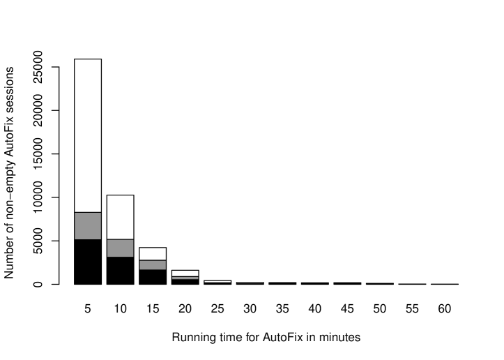
Figure 14: Distribution of running times for AutoFix, independent of the length of the preliminary AutoTest sessions (black bars: sessions with proper fixes; gray bars: sessions with valid fixes; white bars: all sessions).

Table 15 presents the same data about non-empty fixing sessions in a different form: for each amount of AutoFix running time (first column), it displays the number and percentage of sessions that terminated in that amount of time (#Sessions), the number and percentage of those that produced a valid fix (#Valid), and the number and percentage of those that produced a proper fix (#Proper).

Table 15: Distribution of running times for AutoFix.

min. Fixing			#Sessions		#Valid		#Proper
	$5$		25905	(59.7%)	8275	(31.9%)	5130	(19.8%)
	$10$		36164	(83.4%)	13449	(37.2%)	8246	(22.8%)
	$15$		40388	(93.1%)	16220	(40.2%)	9892	(24.5%)
	$20$		42003	(96.9%)	17114	(40.7%)	10432	(24.8%)
	$25$		42436	(97.9%)	17295	(40.8%)	10543	(24.8%)
	$30$		42650	(98.4%)	17371	(40.7%)	10607	(24.9%)
	$40$		43025	(99.2%)	17670	(41.1%)	10799	(25.1%)
	$50$		43318	(99.9%)	17918	(41.4%)	11013	(25.4%)
	$60$		43365	(100.0%)	17954	(41.4%)	11046	(25.5%)

Table 16 shows the minimum, maximum, mean, median, standard deviation, and skewness of the running times (in minutes) across: all fixing sessions, all non-empty sessions, all sessions that produced a valid fix, and all sessions that produced a proper fix.

Table 16: AutoFix running time statistics (times are in minutes).

	min	max	mean	median	stddev	skew
All	0.0	60	4.8	3.0	6.3	3.2
Non-empty	0.0	60	6.1	4.0	6.5	3.2
Valid	0.5	60	7.8	5.5	7.6	2.8
Proper	0.5	60	8.1	5.4	8.3	2.9

Total time per fix.

The total running time of a fixing session also depends on the time spent generating input test cases; the session will then produce a variable number of valid fixes ranging between zero and ten (remember that we ignore fixes not ranked within the top 10). To have a finer-grained measure of the running time based on these factors, we define the unit fixing time of a combined session that runs AutoTest for $t_{1}$ and AutoFix for $t_{2}$ and produces $v>0$ valid fixes as $(t_{1}+t_{2})/v$. Figure 17 shows the distribution of unit fixing times in the experiments: a bar at position $x$ reaching height $y$ denotes that $y$ sessions produced at least one valid fix each, spending an average of $x$ minutes of testing and fixing on each. The distribution is strongly skewed towards short fixing times, showing that the vast majority of valid fixes is produced in 15 minutes or less. Table 19 shows the statistics of unit fixing times for all sessions producing valid fixes, and for all sessions producing proper fixes. Figure 18 shows the same distribution of unit fixing times as Figure 17 but for proper fixes. This distribution is also skewed towards shorted fixing times, but much less so than the one in Figure 17: while the majority of valid fixes can be produced in 35 minutes or less, proper fixes require more time on average, and there is a substantial fraction of proper fixes requiring longer times up to about 70 minutes.

Figure 17: Distribution of unit fixing times for valid fixes (which including the time spent in the preliminary AutoTest sessions).

Figure 18: Distribution of unit fixing times for proper fixes (including the time spent in the preliminary AutoTest sessions).

Table 19: Unit fixing times statistics (times are in minutes and include the time spent in the preliminary AutoTest sessions).

	min	max	mean	median	stddev	skew
Valid	0.7	98.6	10.8	6.9	12.1	2.9
Proper	1.0	101.1	23.5	17.9	17.9	1.1

The unit fixing time is undefined for sessions producing no fixes, but we can still account for the time spent by fruitless fixing sessions by defining the average unit fixing time of a group of sessions as the total time spent testing and fixing divided by the total number of valid fixes produced (assuming we get at least one valid fix). Table 20 shows, for each choice of testing time, the average unit fixing time for valid fixes (second column) and for proper fixes (third column); the last line reports the average unit fixing time over all sessions: 19.9 minutes for valid fixes and 74.2 minutes for proper fixes.

Table 20: Average unit fixing times for different testing times (times are in minutes).

min. Testing	min. Valid	min. Proper
$5$	6.0	22.0
$10$	8.9	32.5
$15$	11.9	43.7
$20$	14.6	54.0
$25$	17.7	65.3
$30$	20.4	76.7
$40$	26.1	97.3
$50$	31.9	121.6
$60$	37.3	143.5
All	19.9	74.2

Looking at the big picture, the fixing times are prevalently of moderate magnitude, suggesting that AutoFix (and its usage in combination with AutoTest) can make an efficient usage of computational time and quickly produce useful results in most cases. The experimental results also suggest practical guidelines to use AutoFix and AutoTest: as a rule of thumb, running AutoTest for five to ten minutes has a fair chance of producing test cases for AutoFix to correct an “average” fault.

In our experiments, AutoFix took on average less than
20 minutes per valid fix, including the time required
to generate suitable tests with AutoTest.

5.3.4 Robustness

The last part of the evaluation analyzes the robustness and repeatability of AutoFix sessions. The AutoFix algorithm is purely deterministic, given as input an annotated program and a set of passing and failing test cases exposing a fault in the program. In our experiments, however, all the tests come from AutoTest, which operates a randomized algorithm, so that different runs of AutoTest may produce test suites of different quality. We want to assess the robustness of AutoFix with respect to different choices of input test suites, that is how AutoFix’s output depends on the test cases supplied. Assessing robustness is important to demonstrate that our evaluation is indicative of average usage, and its results do not hinge on having used a particularly fortunate selection of tests.

Our experiments consisted of many repeated runs of AutoTest, each followed by AutoFix runs using the generated test as input. To assess robustness we fix the testing time, and we measure the percentage of AutoFix runs, on each of the repeated testing sessions terminating within the allotted testing time, that produced a valid fix. A high percentage shows that AutoFix was successful in most of the repeated testing runs, and hence largely independent of the specific performance of AutoTest; to put it differently, a random testing session followed by a fixing sessions has a high chance of producing a valid fix.

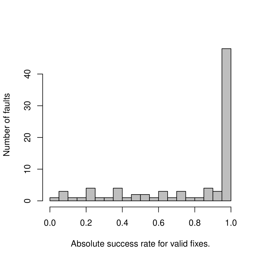
(a) Absolute success rate.

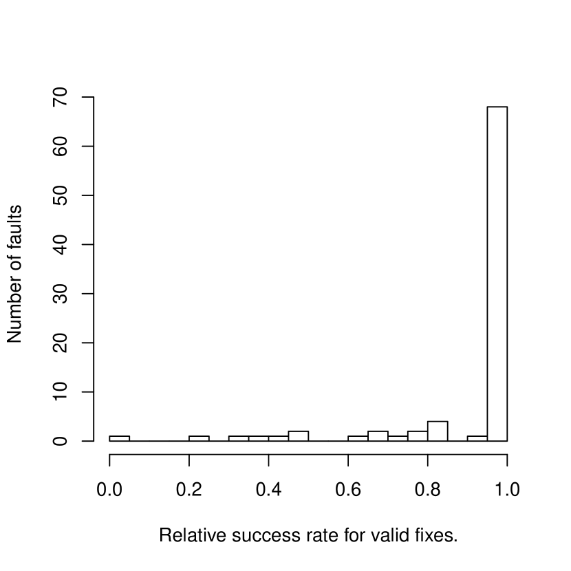
(b) Relative success rate.

Figure 21: Distribution of success rates for valid fixes.

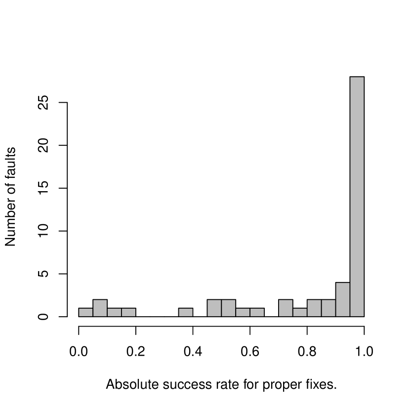
(a) Absolute success rate.

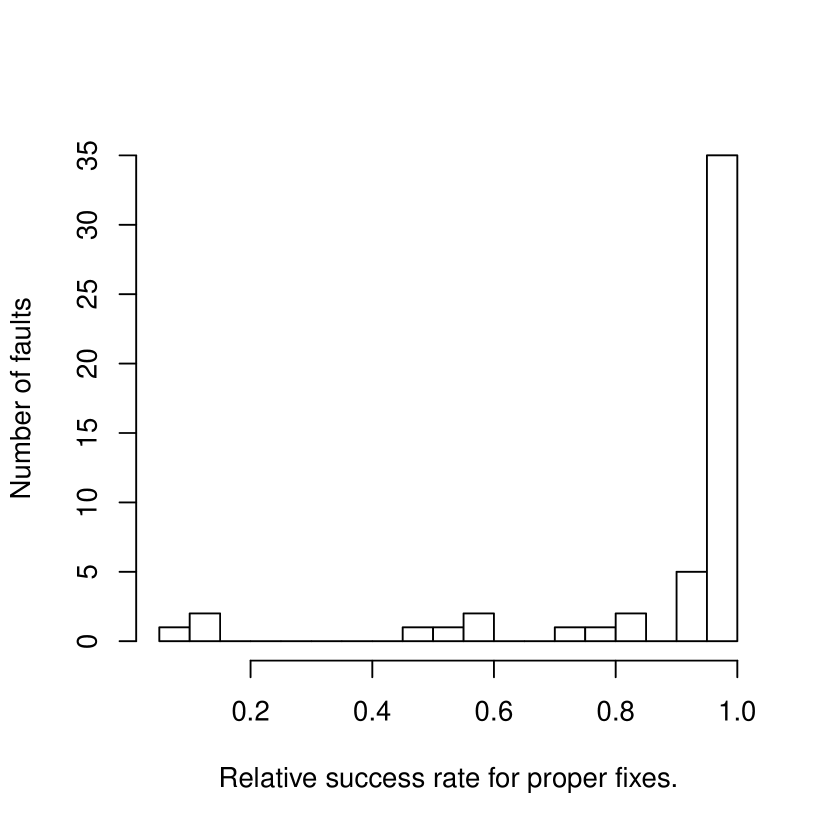
(b) Relative success rate.

Figure 22: Distribution of success rates for proper fixes.

Formally, to measure the robustness with respect to choice of test cases, we introduce the notion of success rate: given a fault $\mathfrak{f}$ and a testing time $m$, the $m$-minute absolute success rate on $\mathfrak{f}$ is defined as the percentage of $m$-minute fixing sessions on $\mathfrak{f}$ that produce at least one valid fix; the relative success rate is defined similarly but the percentage is relative only to non-empty fixing sessions (where AutoTest produced at least one failing test case). Figure 21 shows the distribution of the absolute (Figure 21(a)) and relative (Figure 21(b)) success rates for all “fixable” faults—for which AutoFix produced a valid fix at least once in our experiments—for any testing time $m$. The graphs demonstrate that AutoFix has repeatable behavior with a strong majority of faults, largely insensitive to the specific input test cases. The relative success rates, in particular, exclude the empty AutoTest sessions (which are concentrated on some “hard to reproduce faults” as discussed in Section 5.3.1) and thus characterize the robustness of AutoFix’s behavior on the “approachable” faults. (The fact that a classification into “approachable” and “hard” faults for AutoFix naturally emerges further indicates that the kinds of faults used in this evaluation are varied.)

To have a quantitative look at the same data, Table 23 displays, for each testing time $m$, the number of faults that were fixed successfully—producing a valid fix—in at least $X\%$ of the $m$-minute fixing sessions, for percentages $X=50,80,90,95$. Each table entry also shows, in parentheses, the percentage of the fixed faults, relative to the 86 fixable faults that AutoFix fixed at least once; the data is shown for both the relative and the absolute success rate. For example, AutoFix was successful at least 95% of the times with 56% of all fixable faults; or even with 79% of all fixable faults provided with at least one failing test case. The last line displays the statistics over all testing sessions of any length. The aggregated data over all fixing sessions for all faults is the following: 32% of all sessions and 41% of all non-empty sessions produced a valid fix. These success rates suggest a high repeatability of fixing.

Figure 22 and Table 24 display similar data about successful sessions that produced at least one proper fix, with percentages relative to all faults for which AutoFix produced a proper fix at least once in our experiments. The aggregated data over all fixing sessions for all faults is the following: 20% of all sessions and 25% of all non-empty sessions produced a proper fix; these percentages are quite close to the 25% of all faults for which AutoFix produces at least once a proper fix (Table 12). The data for proper fixes is overall quite similar to the one for valid fixes. The absolute figures are a bit smaller, given that the requirement of proper fixes is more demanding, but still support the hypothesis that AutoFix’s behavior is often robust and largely independent of the quality of provided test cases.

Table 23: Repeatability of AutoFix on faults that produced some valid fixes.

Success rate:	50%				80%				90%				95%
min. Testing	relative		absolute		relative		absolute		relative		absolute		relative		absolute
5	83	(97%)	58	(67%)	80	(93%)	49	(57%)	78	(91%)	46	(53%)	75	(87%)	40	(47%)
10	83	(97%)	62	(72%)	77	(90%)	56	(65%)	75	(87%)	51	(59%)	69	(80%)	45	(52%)
15	81	(94%)	65	(76%)	76	(88%)	58	(67%)	71	(83%)	52	(60%)	68	(79%)	48	(56%)
20	82	(95%)	68	(79%)	76	(88%)	58	(67%)	70	(81%)	54	(63%)	67	(78%)	51	(59%)
25	80	(93%)	68	(79%)	72	(84%)	58	(67%)	70	(81%)	56	(65%)	65	(76%)	51	(59%)
30	81	(94%)	69	(80%)	74	(86%)	59	(69%)	70	(81%)	56	(65%)	68	(79%)	53	(62%)
40	79	(92%)	69	(80%)	71	(83%)	61	(71%)	68	(79%)	58	(67%)	65	(76%)	55	(64%)
50	79	(92%)	70	(81%)	73	(85%)	62	(72%)	69	(80%)	59	(69%)	63	(73%)	53	(62%)
60	78	(91%)	71	(83%)	73	(85%)	61	(71%)	68	(79%)	59	(69%)	67	(78%)	57	(66%)
All	79	(92%)	67	(78%)	73	(85%)	56	(65%)	69	(80%)	51	(59%)	68	(79%)	48	(56%)

Table 24: Repeatability of AutoFix on faults that produced some proper fixes.

Success rate:	50%				80%				90%				95%
min. Testing	relative		absolute		relative		absolute		relative		absolute		relative		absolute
5	45	(88%)	35	(69%)	42	(82%)	31	(61%)	41	(80%)	41	(80%)	39	(76%)	24	(47%)
10	47	(92%)	41	(80%)	43	(84%)	35	(69%)	42	(82%)	42	(82%)	36	(71%)	27	(53%)
15	47	(92%)	41	(80%)	43	(84%)	37	(73%)	39	(76%)	39	(76%)	36	(71%)	29	(57%)
20	47	(92%)	43	(84%)	43	(84%)	37	(73%)	40	(78%)	40	(78%)	35	(69%)	27	(53%)
25	48	(94%)	44	(86%)	42	(82%)	37	(73%)	39	(76%)	39	(76%)	34	(67%)	28	(55%)
30	46	(90%)	43	(84%)	42	(82%)	37	(73%)	41	(80%)	41	(80%)	39	(76%)	32	(63%)
40	47	(92%)	45	(88%)	41	(80%)	39	(76%)	39	(76%)	39	(76%)	34	(67%)	32	(63%)
50	47	(92%)	45	(88%)	42	(82%)	39	(76%)	39	(76%)	39	(76%)	33	(65%)	31	(61%)
60	47	(92%)	45	(88%)	41	(80%)	39	(76%)	40	(78%)	40	(78%)	34	(67%)	31	(61%)
All	47	(92%)	43	(84%)	42	(82%)	36	(71%)	40	(78%)	40	(78%)	35	(69%)	28	(55%)

In our experiments, AutoFix produced valid fixes
in 41% of the sessions with valid input tests.

5.4 Limitations and threats to validity

Limitations.

AutoFix relies on a few assumptions, which may restrict its practical applicability.

Contracts or a similar form of annotation must be available in the source code. The simple contracts that programmers write [32] are sufficient for AutoFix; and having to write contracts can be traded off against not having to write test cases. Requiring contracts does not limit the applicability of our technique to Eiffel, given the increasing availability of support for contracts in mainstream programming languages. However, the software projects that use contracts in their development is still a small minority [32], which restricts broader applicability of AutoFix on the software that is currently available without additional annotation effort.

Whether writing contracts is a practice that can become part of mainstream software development is a long-standing question. Our previous experience is certainly encouraging, in that using contracts does not require highly-trained programmers, and involves efforts that can be traded off against other costs (e.g., maintenance [63]) and are comparable to those required by other more accepted practices. For example, EiffelBase’s contracts-to-code ratio is around 0.2 [82]; while detailed quantitative data about industrial experiences with a more accepted practice such as test-driven development is scarce, the few references that indicate quantitative measures [12, 64, 57] report test-LOC-to-application-LOC ratios between 0.4 and 1.0 for projects of size comparable to EiffelBase. More extensive assessments belong to future work beyond the scope of the present paper.

Functional faults are the primary target of AutoFix, given that contracts provide an effective specification of functional correctness. This excludes, for example, violation of liveness properties (e.g., termination) or low-level I/O runtime errors (Section 5.2.1). Nonetheless, the expressiveness of contracts is significant, and in fact we could identify various categories of contract-violation faults that AutoFix can or cannot fix (Section 5.3.1).

Correctness of contracts is assumed by AutoTest, which uses them as oracles, and by AutoFix, which fixes implementations accordingly. Since contracts have errors too, this may affect the behavior of AutoFix on certain faults (see Section 5.3.1). Anyway, the line for correctness must be drawn somewhere: test cases may also include incorrect usages or be incorrectly classified.

Types of fixes generated by AutoFix include only a subset of all possible actions (Section 4.3) and are limited to simple schema (Section 4.4). This limits the range of fixes that AutoFix can generate; at the same time, it helps reduce the search space of potential fixes, focusing on the few schema that cover the majority of cases [24, 56].

Threats to validity.

While we designed the evaluation of AutoFix targeting a broad scope and repeatable results, a few threats to generalizability remain.

Automatically generated test cases were used in all our experiments. This provides complete automation to the debugging process, but it also somewhat restricts the kinds of projects and the kinds of faults that we can try to those that we can test with AutoTest. We plan to experiment with manually-written test cases in future work.

Unit tests were used in all our experiments, as opposed to system tests. Unit tests are normally smaller, which helps with fault localization and, consequently, to reduce the search space of possible fixes. The fact that unit tests are produced as part of fairly widespread practices such as test-driven development [12] reflects positively on the likelihood that they be available for automated fixing.

Size and other characteristics (type of program, programming style, and so on) of the programs used in the evaluation were constrained by the fundamental choice of targeting object-oriented programs using contracts that can be tested with AutoTest. This implies that further experiments are needed to determine to what extent the algorithms used by AutoFix scale to much larger code bases—possibly with large-size modules and system-wide executions—and which design choices should be reconsidered in that context. To partly mitigate this threat to generalizability, we selected experimental subjects of non-trivial size exhibiting variety in terms of quality, maturity, and available contracts—within the constraints imposed by our fundamental design choices, as discussed in Section 5.2.1.

Variability of performance relative to different choices for the various heuristics used by AutoFix has not been exhaustively investigated. While most heuristics rely on well-defined notions, and we provided the rationale for the various design choices, there are a few parameters (such as $\alpha$, $\beta$, and $\gamma$ in Section 4.2.2) whose impact we have not investigated as thoroughly as other aspects of the AutoFix algorithm. As also discussed in Section 4.2.2, the overall principles behind the various heuristics are not affected by specific choices for these parameters; therefore, the impact of this threat to generalizability is arguably limited.

Limited computational resources were used in all our experiments; this is in contrast to other evaluations of fixing techniques [46]. Our motivation for this choice is that we conceived AutoFix as a tool integrated within a personal development environment, usable by individual programmers in their everyday activity. While using a different approach to automatic fixing could take advantage of massive computational resources, AutoFix was designed to be inexpensive and evaluated against this yardstick.

Classification of fixes into proper and improper was done manually by the first author. While this may have introduced a classification bias, it also ensured that the classification was done by someone familiar with the code bases, and hence in a good position to understand the global effects of suggested fixes. Future work will investigate this issue empirically, as done in recent related work [45].

Programmer-written contracts were used in all our experiments. This ensures that AutoFix works with the kinds of contracts that programmers tend to write. However, as future work, it will be interesting to experiment with stronger higher-quality contracts to see how AutoFix performance is affected. In recent work [82] we obtained good results with this approach applied to testing with AutoTest.

6 Related work on automated fixing

We present the related work on automated program fixing in three areas: techniques working on the source code (as AutoFix does); applications to specialized domains; and techniques that operate dynamically at runtime.

6.1 Source-code repairs

Techniques such as AutoFix target the source code to permanently remove the buggy behavior from a program.

Machine-learning techniques.

Machine-learning techniques can help search the space of candidate fixes efficiently and support heuristics to scale to large code bases.

Jeffrey et al. [41] present BugFix, a tool that summarizes existing fixes in the form of association rules. BugFix then tries to apply existing association rules to new bugs. The user can also provide feedback—in the form of new fixes or validations of fixes provided by the algorithm—thus ameliorating the performance of the algorithm over time.

Other authors applied genetic algorithms to generate suitable fixes. Arcuri and Yao [10, 7] use a co-evolutionary algorithm where an initially faulty program and some test cases compete to evolve the program into one that satisfies its formal specification.

Weimer et al. [95, 94] describe GenProg, a technique that uses genetic programming to mutate a faulty program into one that passes all given test cases. GenProg has been extensively evaluated [47, 46] with various open-source programs, showing that it provides a scalable technique, which can produce non-trivial corrections of subtle bugs, and which works without any user annotations (but it requires a regression test suite).

Kim et al. [45] describe Par, a technique that combines GenProg’s genetic programming with a rich predefined set of fix patterns (suggested by human-written patches). Most of the fix patterns supported by Par are covered by AutoFix’s synthesis strategies (Section 4.3); the few differences concern the usage of overloaded methods—a feature not available in the Eiffel language, and hence not covered by AutoFix. Par has also been extensively evaluated, with a focus on acceptability of patches: the programmers involved in the study tended to consider the patches generated by Par more acceptable than those generated by GenProg, and often as acceptable as human-written patches for the same bugs. The notion of acceptability addresses similar concerns to our notion of proper fix, since they both capture quality as perceived by human programmers beyond the objective yet weak notion of validity, although the two are not directly comparable.

Of the several approaches to source-code general-purpose program repair discussed in this section, GenProg and Par are the only ones that have undergone evaluations comparable with AutoFix’s: the other approaches have only been applied to seeded faults [37, 35, 7], to few benchmarks used for fault localization [41], or do not aim at complete automation [93].

GenProg can fix 52% of 105 bugs with the latest improvements [46]; Par fixes 23% of 119 bugs (GenProg fixes 13% of the same 119 bugs [45]). In our experiments in Section 5, we target almost twice as many bugs (204) and AutoFix fixes 42% of them. Whereas these quantitative results should not directly be compared because they involve different techniques and faults, they demonstrate that all three approaches produce interesting results and have been thoroughly evaluated. GenProg’s and Par’s evaluations have demonstrated their scalability to large programs: GenProg worked on 8 C programs totaling over 5 million lines of code; Par worked on 6 Java programs totaling nearly 500 thousand lines of code. AutoFix’s evaluation targeted a total of 72 thousand lines of Eiffel code; while lines of code is a coarse-grained measure of effort, more experiments are needed to conclusively evaluate AutoFix’s scalability on much larger programs. The test cases used in GenProg’s and Par’s evaluations (respectively, around 10 thousand and 25 thousand) do not seem to be directly comparable with those used by AutoFix: GenProg and Par use manually-written tests, which may include system tests as well as unit tests; AutoFix does not require user-written test cases (and uses fewer on average anyway) but uses automatically generated tests that normally exercise only a limited subset of the instructions in the whole program. The sensitivity of GenProg or Par about the input test suite have not been systematically investigated, and therefore we do not know if they could perform well with tests generated automatically. In contrast, our experiments show that AutoFix is robust with respect to the input tests, and in fact it works consistently well with tests randomly generated given the simple contracts available in Eiffel programs. Another advantage of leveraging contracts is that AutoFix can naturally target functional errors (such as those shown in Section 2).

Weimer et al.’s evaluation of fix quality has been carried out only for a sample of the bugs, and mostly in terms of induced runtime performance [47]. It is therefore hard to compare with AutoFix’s. Finally, AutoFix works with remarkably limited computational resources: using the same pricing scheme used in GenProg’s evaluation [46], AutoFix would require a mere $0.01 per valid fix (computed as $0.184\times\text{total fixing time in hours}\>/\>\text{total number of valid fixes}$) and $0.03 per proper fix; or $0.06 per valid and $0.23 per proper fix including the time to generate tests—two orders of magnitude less than GenProg’s $7.32 per valid fix.

Axiomatic reasoning.

He and Gupta [37] present a technique that compares two program states at a faulty location in the program. The comparison between the two program states illustrates the source of the error; a change to the program that reconciles the two states fixes the bug. Unlike our work, theirs compares states purely statically with modular weakest precondition reasoning. A disadvantage of this approach is that modular weakest precondition reasoning may require detailed postconditions (typically, full functional specifications in first-order logic) in the presence of routine calls: the effects of a call to foo within routine bar are limited to what foo’s postcondition specifies, which may be insufficient to reason about bar’s behavior. Even if the static analysis were done globally instead of modularly, it would still require detailed annotations to reason about calls to native routines, whose source code is not available. This may limit the applicability to small or simpler programs; AutoFix, in contrast, compares program states mostly dynamically, handling native calls and requiring only simple annotations for postconditions. Another limitation of He and Gupta’s work is that it builds fix actions by syntactically comparing the two program states; this restricts the fixes that can be automatically generated to changes in expressions (for example, in off-by-one errors). AutoFix uses instead a combination of heuristics and fix schemas, which makes for a flexible usage of a class’s public routines without making the search space of possible solutions intractably large.

Constraint-based techniques.

Gopinath et al. [35] present a framework that repairs errors due to value misuses in Java programs annotated with pre- and postconditions. A repairing process with the framework involves encoding programs as relational formulae, where some of the values used in “suspicious” statements are replaced by free variables. The conjunction of the formula representing a program with its pre- and postcondition is fed to a SAT solver, which suggests suitable instantiations for the free variables. The overall framework assumes an external fault localization scheme to provide a list of suspicious statements; if the localization does not select the proper statements, the repair will fail. Solutions using dynamic analysis, such as AutoFix, have a greater flexibility in this respect, because they can better integrate fault localization techniques—which are also typically based on dynamic analysis. As part of future work, however, we will investigate including SAT-based techniques within AutoFix.

Nguyen et al. [65] build on previous work [17] about detecting suspicious expressions to automatically synthesize possible replacements for such expression; their SemFix technique replaces or adds constants, variables, and operators to faulty expressions until all previously failing tests become passing. The major differences with respect to AutoFix are that SemFix’s fault localization is based on statements rather than snapshots, which gives a coarser granularity; and that the fixes produced by SemFix are restricted to changes of right-hand sides of assignments and Boolean conditionals, whereas AutoFix supports routine calls, more complex expression substitutions, and conditional schemas. This implies that AutoFix can produce fixes that are cumbersome or impossible to build using SemFix. For example, conditional fixes are very often used by AutoFix (Tables 11 and 13) but can be generated by SemFix only if a conditional already exists at the repair location; and supporting routine calls in fixes takes advantage of modules with a well-designed API.

Model-driven techniques.

Some automated fixing methods exploit finite-state abstractions to detect errors or to build patches. AutoFix also uses a form of finite-state abstraction as one way to synthesize suitable fixing actions (Section 4.3.3).

In previous work, we developed Pachika [23], a tool that automatically builds finite-state behavioral models from a set of passing and failing test cases of a Java program. Pachika also generates fix candidates by modifying the model of failing runs in a way which makes it compatible with the model of passing runs. The modifications can insert new transitions or delete existing transitions to change the behavior of the failing model; the changes in the model are then propagated back to the Java implementation. AutoFix exploits some of the techniques used in Pachika—such as finite-state models and state abstraction—in combination with other novel ones—such as snapshots, dynamic analysis for fault localization, fix actions and schema, contracts, and automatic test-case generation.

Weimer [93] presents an algorithm to produce patches of Java programs according to finite-state specifications of a class. The main differences with respect to AutoFix are the need for user-provided finite-state machine specifications, and the focus on security policies: patches may harm other functionalities of the program and “are not intended to be applied automatically” [93].

6.2 Domain-specific models

Automated debugging can be more tractable over restricted models of computations. A number of works deal with fixing finite-state programs, and normally assumes a specification given in some form of temporal logic [58, 43, 43].

Gorla et al. [16, 36] show how to patch web applications at runtime by exploiting the redundancy of services offered through their APIs; the patches are generated from a set of rewrite rules that record the relations between services. In more recent work [15], they support workarounds of general-purpose Java applications based on a repertoire of syntactically different library calls that achieve the same semantics.

Janjua and Mycroft [40] target atomicity violation errors in concurrent programs, which they fix by introducing synchronization statements automatically. More recently, Jin et al. [42] developed the tool AFix that targets the same type of concurrency errors.

Abraham and Erwig [1] develop automated correction techniques for spreadsheets, whose users may introduce erroneous formulae. Their technique is based on annotating cells with simple information about their “expected value”; whenever the computed value of a cell contradicts its expected value, the system suggests changes to the cell formula that would restore its value to within the expected range. The method can be combined with automated testing techniques to reduce the need for manual annotations [2].

Samimi et al. [87] show an approach to correct errors in print statements that output string literals in PHP applications. Given a test suite and using an HTML validator as oracle for acceptable output, executing each test and validating its output induces a partial constraint on the string literals. Whenever the combination of all generated constraints has a solution, it can be used to modify the string literals in the print statements to avoid generating incorrect output. Constraint satisfaction can be quite effective when applied to restricted domains such as PHP strings; along the same lines, AutoFix uses constraint-based techniques when dealing with linear combinations of integer variables (Section 4.3.4).

6.3 Dynamic patching

Some fixing techniques work dynamically, that is at runtime, with the goal of contrasting the adverse effects of some malfunctioning functionality and prolonging the up time of some piece of deployed software. Demsky et al. [26, 28] provide generic support for dynamic patching inside the Java language.

Data-structure repair.

Demsky and Rinard [27] show how to dynamically repair data structures that violate their consistency constraints. The programmer specifies the constraints, which are monitored at runtime, in a domain language based on sets and relations. The system reacts to violations of the constraints by running repair actions that try to restore the data structure in a consistent state.

Elkarablieh and Khurshid [29] develop the Juzi tool for Java programs. A user-defined repOk Boolean query checks whether the data structure is in a coherent state. Juzi monitors repOk at runtime and performs some repair action whenever the state is corrupted. The repair actions are determined by symbolic execution and by a systematic search through the object space. In follow-up work [54, 55], the same authors outline how the dynamic fixes generated by Juzi can be abstracted and propagated back to the source code.

Samimi et al.’s work [86] leverages specifications in the form of contracts to dynamically repair data structures and other applications. As in our work, an operation whose output violates its postcondition signals a fault. When this occurs, their Plan B technique uses constraint solving to generate a different output for the same operation that satisfies the postcondition and is consistent with the rest of the program state; in other words, they execute the specification as a replacement for executing a faulty implementation. Their prototype implementation for Java has been evaluated on a few data-structure faults similar to those targeted by Demsky and Rinard [27], as well as on other operations that are naturally expressed as constraint satisfaction problems.

Memory-error repair.

The ClearView framework [78] dynamically corrects buffer overflows and illegal control flow transfers in binaries. It exploits a variant of Daikon [31] to extract invariants in normal executions. When the inferred invariants are violated, the system tries to restore them by looking at the differences between the current state and the invariant state. ClearView can prevent the damaging effects of malicious code injections.

Exterminator [13, 67] is a framework to detect and correct buffer overflow and dangling pointer errors in C and C++ programs. The tool executes programs using a probabilistic memory allocator that assigns a memory area of variably larger size to each usage; an array of size $n$, for example, will be stored in an area with strictly more than $n$ cells. With this padded memory, dereferencing pointers outside the intended frame (as in an off-by-one overflow access) will not crash the program. Exterminator records all such harmless accesses outside the intended memory frame and abstracts them to produce patches that permanently change the memory layout; the patched layout accommodates the actual behavior of the program in a safe way.

7 Conclusions

In the past decade, automated debugging has made spectacular advances: first, we have seen methods to isolate failure causes automatically; then, methods that highlight likely failure locations. Recently, the slogan “automated debugging” has denoted techniques that truly deserve this name: we can actually generate workable fixes completely automatically.

The AutoFix approach, described in the paper, is an important contribution towards the ideal of automatic debugging. In experiments with over 200 faults in software of various quality, AutoFix generated fixes for 42% of the faults; inspection reveals 59% of them are not mere patches but real corrections of quality comparable to those programmers familiar with the faulty programs could write. AutoFix achieves these results with limited computational resources: running on standard hardware, it required an average time per fix under 20 minutes—where the average includes all failed fixing attempts and the automatic generation of test cases that profile the faults. One of the key ingredients used to achieve these encouraging results is the reliance on contracts to boost and automate all debugging steps. The kinds of contracts required by AutoFix are simple and normally available in Eiffel programs; the effort of writing them is, therefore, limited and comparable to other everyday programming activities.

With AutoFix, the programmer’s debugging effort could be reduced to almost zero in many cases. We write “almost zero”, as we still assume that a human should assess the generated fixes and keep authority over the code. One may also think of systems that generate and apply fixes automatically; the risk of undesired behavior may still be preferred to no behavior at all, and can be alleviated by more precise specifications expressed as contracts. In any case, we look forward to a future in which much of the debugging is taken over by automated tools, reducing risks in development and relieving programmers from a significant burden.

Availability. The AutoFix source code, and all data and results cited in this article, are available at:

http://se.inf.ethz.ch/research/autofix/

Acknowledgments. This work was partially funded by the Hasler-Stiftung (Grant no. 2327) and by the Deutsche Forschungsgemeinschaft (Ze509/4-1) under the title “AutoFix—Programs that fix themselves”; and by the Swiss National Science Foundation (Project 200021-134976: “Automated Support for Invariant Inference”). We also gratefully acknowledge the support of the Swiss National Supercomputing Centre (CSCS) for the experiments (Project s264). The concept of generating fixes from differences in passing and failing runs was conceived with Andreas Leitner. Stefan Buchholz and Lucas S. Silva contributed to an early implementation of AutoFix.

This Appendix contains additional material omitted from the referred main text. The section titles correspond to those in the main text where the additional material belongs; for greater clarity, the titles also mention, in parentheses, the corresponding section numbers in the main text, when they exist.

Appendix A AutoFix in action (Section 2)

A.1 Another error in move_item (Section 2.2)

Another error occurs when index has value 0 (Figure 25(a)), meaning that before (line 5) has value True; this is a valid position for go_i_th but not for put_left, because there is no position “to the left of 0” where v can be re-inserted: the call to put_left on line 42 violates its precondition (line 26).

(a) Calling put_left in move_item when index = 0 triggers a failure: there is no valid position to the left of $0$ where $v$ can be moved.

(b) The cursor index is on the boundary position count + 1. Calling remove in move_item will remove the element $v$ inside the list without updating index.

(c) After removing the item containing v, count is decremented. Thus, the cursor index points to the invalid position count + 2.

Figure 25: Two faults violating contracts in move_item. In the first fault (25(a)), index is initially “before”. In the second fault (25(b)–25(c)), index is initially in position count + 1 (25(b)), a position which becomes invalid after removing an element inside the list (25(c)).

A.2 Automatic corrections of the errors in move_item (Section 2.3)

AutoFix collects the test cases generated by AutoTest that exercise routine move_item. Based on them, and on other information gathered by dynamic and static analysis, it produces, after running only a few minutes on commodity hardware without any user input, up to 10 suggestions of fixes for each of the two errors discussed. The suggestions include only valid fixes: fixes that pass all available tests targeting move_item. Among them, we find the two “proper” fixes in Figure A.2, which completely correct the errors in a way that makes us confident enough to deploy them in the program.

⬇ 57if before then 58 forth 59end

⬇ 57if idx $>$ index then 58 idx := idx - 1 59end

Figure 26: Corrections of the two errors in move_item automatically generated by AutoFix.

The correction for error occurring when calling put_left with index = 0) consists of inserting the lines 57–59 in Figure A.2 (left) before the call to put_left on line 42 in Figure 2. When before holds (i.e., index is 0), calling forth moves the cursor to position 1, which is valid for put_left and is where v is inserted. This behavior follows a reasonable interpretation of what it means to insert an element “to the left of cursor” when the cursor is already in the leftmost position: insert the element in the leftmost position.

The correction for the other error (occurring when v is initially in a position to the left of index) consists of inserting the lines 43–45 in Figure A.2 (right) before the call to go_i_th on line 41 in Figure 2. The condition idx $>$ index holds precisely when v was initially in a position to the left of index ; in this case, we must decrement idx by one to accommodate the decreased value of count after the call to remove. This fix completely corrects this error beyond the specific case in Figure 25 reported by AutoTest, even though move_item has no postcondition that formalizes its intended behavior.

AutoFix’s suggestions for the two errors include other fixes that managed to pass all available tests. Among the 10 suggestions for the error of calling put_left with index = 0, AutoFix produces two fixes semantically equivalent to the one in Figure A.2; for example, it may use index = 0 instead of before, but the two expressions are equivalent. The remaining seven suggestions for the same error include fixes that avoid the failure and are consistent with the available contracts, but they arguably fail to completely capture the intended implicit semantics of move_item. One of these fixes suggests to replace line 42 in Figure 2 with if not before then put_left (v) end: call put_left only when its precondition is satisfied; otherwise, just discard the element v. The original intent of the programmer implementing move_item probably did not contemplate this behavior as acceptable; therefore, we call fixes such as this one improper. Section 4.5 gives a more rigorous definition of proper fix, and Section 5.3.2 discusses how many of the fixes generated by AutoFix are proper.

Appendix B Experimental evaluation (Section 5)

B.1 Experimental subjects (Section 5.2.1)

Table 27 presents the same information as Table 7 averaged over the number of classes.

Table 27: Average size and other metrics of the code bases.

Code base	$\frac{\textbf{\#kLOC}}{\textbf{\#C}}$		$\frac{\textbf{\#R}}{\textbf{\#C}}$		$\frac{\textbf{\#Q}}{\textbf{\#C}}$		$\frac{\textbf{\#Pre}}{\textbf{\#C}}$		$\frac{\textbf{\#Post}}{\textbf{\#C}}$		$\frac{\textbf{\#Inv}}{\textbf{\#C}}$
Base	2.	4	136.	7	15.	4	104.	3	115.	5	19.	0
TxtLib	1.	2	78.	0	4.	8	9.	7	13.	4	1.	1
Cards	0.	6	46.	2	2.	5	4.	9	18.	3	1.	8
ELearn	0.	5	39.	1	0.	7	5.	3	5.	5	1.	4
Total	0.	9	60.	2	4.	0	19.	3	26.	7	4.	0

B.2 Experimental results (Section 5.3)

Section B.2.1 is a preliminary discussion of how often AutoTest provided tests of good quality suitable for fixing.

B.2.1 Testability of the experimental subjects

For the evaluation, what matters most is the number and quality of fixed produced by AutoFix. It is interesting, however, to look into the results of AutoTest sessions to get a more precise characterization of the experimental subjects and to see how the four code bases differ in their testability. The data provides more evidence that the four code bases have different quality and are diverse subjects for our experiments.

(a) Base

(b) TxtLib

(c) Cards

(d) ELearn

(e) All code bases

Figure 28: Number of tests generated by AutoTest on the experimental subjects.

Total number of tests.

Each histogram in Figure 28 depicts the distribution of the mean number of test cases generated by AutoTest in the 30 repeated 60-minute sessions for each routine. That is, a bar at position $x$ reaching height $y$ denotes that there exist $y$ routines $r_{1},\ldots,r_{y}$ such that, for each $1\leq j\leq y$, the mean number $|T|$ of tests $T$ in the 60-minute series on some fault of $r_{j}$ is $x$. Figures 28(a)–28(d) show the distributions of the individual code bases, while Figure 28(e) is the overall distribution.

The figures suggest that Base is normally easily testable—probably a consequence of its carefully-designed interface and contracts. In contrast, Cards and ELearn are hard to test on average; and TxtLib is a mixed case. A Mann-Whitney $U$ test confirms that the differences are statistically significant: if we partition the four code bases into two groups, one comprising Base and TxtLib and the other Cards and ELearn, intra-group differences are not statistically significant (with $692\leq U\leq 1272$ and $p>0.06$) whereas inter-group differences are (with $264\leq U\leq 1754$ and $p<0.03$).

(a) Base

(b) TxtLib

(c) Cards

(d) ELearn

(e) All code bases

Figure 29: Failing-to-passing ratio of tests generated by AutoTest on the experimental subjects; the horizontal scales are logarithmic.

Failing to passing tests.

Another interesting measure is the average ratio of failing to passing tests generated in one session, which gives an idea of how frequent failures are. Each histogram in Figure 29 depicts the distribution of the mean failing-to-passing ratio for the test cases generated by AutoTest in the 30 repeated 60-minute sessions for each routine; notice that the horizontal scale is logarithmic. That is, a bar at position $x$ reaching height $y$ denotes that there exist $y$ routines $r_{1},\ldots,r_{y}$ such that, for each $1\leq j\leq y$, the mean ratio $|F|/|P|$ of failing tests $F$ to passing tests $P$ in the 60-minute series on some fault of $r_{j}$ is $e^{x}$.

Consistently with Figure 28, Figure 29 suggests that it is harder to produce failing tests for Base than for the other code bases. A Mann-Whitney $U$ test confirms that the difference between Base and the other three code bases is statistically significant (with $105\leq U\leq 445$ and $p<10^{-7}$) whereas the differences among TxtLib, Cards, and ELearn are not (with $515\leq U\leq 859$ and $p>0.06$).

Appendix C Related work (Section 6)

AutoFix integrates numerous techniques to detect, locate, and correct programming errors automatically. This section reviews the related work in these areas, focusing on those most closely related and that include an extensive evaluation.

C.1 Fault detection: automatic testing

During the last decade, automatic testing has become an effective technique to detect faults, in programs and systems, completely automatically. Among the approaches to automatic testing, random testing is one of the simplest, yet it has been successfully applied to a variety of programs including Java libraries and applications [70, 22, 88]; Eiffel libraries [19]; and Haskell programs [20]. The research on random testing has produced a variety of tools—including our own AutoTest [61], Randoop [71], JCrasher [22], Eclat [70], Jtest [73], Jartege [68], Yeti [69], and RUTE-J [5]—as well as rigorous analysis [9] justifying its practical success on theoretical grounds.

Search-based test-case generation refines random testing with the goal of improving its performance and accuracy. McMinn [59] and Ali et al. [3] survey the state of the art in search-based techniques. Genetic algorithms are a recurring choice for searching over unstructured spaces in combination with random exploration; Tonella [89] first suggested the idea, and Andrews et al. [6] show how to use genetic algorithms to optimize the performance of standard random testing. Our previous work [90, 92] also extended purely random testing with search-based techniques. Other approaches to automatic testing introduce white-box techniques such as symbolic execution [53] and fuzzying [34], or leverage the availability of formal specifications in various forms [38, 100].

C.2 Fault localization

Fault localization is the process of locating statements that should be changed in order to correct a given fault. Many of the approaches to automated fault localization rely on measures of code coverage or program states.

Code coverage.

Code coverage metrics have been used to rank instructions based on their likelihood of triggering failures. Jones et al. [44], for example, introduce the notion of failure rate: an instruction has a high failure rate if it is executed more often in failing test cases than in passing test cases. A block of code is then “suspicious” of being faulty if it includes many instructions with high failure rate; Jones et al. also implemented visualization support for their debugging approach in the tool Tarantula.

Renieris and Reiss’s fault localization technique [85] is based on the notion of nearest neighbor: given a test suite, the nearest neighbor of a faulty test case $t$ is the passing test case that is most similar to $t$. Removing all the instructions mentioned in the nearest neighbor from the faulty test produces a smaller set of instructions; instructions in the set are the prime candidates to be responsible for the fault under consideration. Artzi et al. [11] apply similar techniques to rank statements together with their runtime values to locate execution faults in PHP web applications. For better fault localization effectiveness, Artzi et al. also exploit concolic test-generation techniques to build new test cases that are similar to the failing one, the basic idea being that the differences between similar passing and failing test executions highly correlate with the fault cause.

Many other authors have extended code coverage techniques for fault localization. For example, Zhang et al. [99] address the propagation of infected program states; Liu et al. [51] rely on a model-based approach; and Wong et al. [96] perform an extensive comparison of variants of fault localization techniques and outline general principles behind them (which we follow in Section 4.2.2). Pytlik et al. [83] discuss the limitations of using only state invariants for fault localization, a limitation that AutoFix avoids by combining snapshots based on state invariants with snapshots based on enumeration (Section 4.1).

Program states.

The application of code coverage techniques produces a set of instructions likely to be responsible for failure; programmers still have to examine each instruction to understand what the problem is. Fault localization techniques based on program states aim at providing more precise information in such contexts: state-based analyses are finer-grained than those based only on code coverage because they can also report suspicious state values that should be changed. Huang et al [39], for example, suggest to insert check points in the program to mark “points of interest”. Then, a dynamic analysis—applied to program states rather than locations—can identify a set of suspicious states; furthermore, the usage of check points introduces the flexibility to skip uninteresting parts of the computation, for example repeated iterations of a loop. Delta debugging [97, 98] addresses similar issues: isolating the variables, and their values, relevant to a failure by analyzing the state difference between passing and failing test cases.

Angelina [17] is a technique that repeatedly runs a program against a group of tests with the intent of discovering a list of expressions from the suspected faulty code such that: changing the value of any such expression at runtime could make the failing tests pass, while still letting the originally passing tests pass. Such expressions are then reported to the programmer as suggestions: building the actual corrections is still the programmer’s job.

Most fault localization techniques target each fault individually, and hence they perform poorly when multiple bugs interact and must be considered together. To address such scenarios, Liblit et al. [49] introduce a technique that separates the effects of multiple faults and identifies predictors associated with each fault.

While the research on automated fault localization has made substantial progresses, effectively applying fault localization in practice to help programmers still poses open challenges. Parnin and Orso [74] demonstrate that most automated debugging techniques focus on tasks (mostly, localization) that represent only a small part of the real debugging activity. Automated fixing techniques can help in this regard by providing an additional layer of automation that includes synthesizing suitable validated corrections.

Fault localization for automatic fixing.

The program fixing techniques of the present paper include fault localization techniques (Section 4.2). To generate fixes completely automatically fault localization must be sufficiently precise to suggest only a limited number of “suspicious” instructions. In our case, using contracts helps to restrict the search to the boundaries of the routine where a contract-violation fault occurs. Then, we combine dynamic analysis techniques based on those employed for fault localization (Section 4.2.2) with simple static analyses (Section 4.2.1) to produce a ranking of state snapshots within routines that is sufficiently accurate for the fixing algorithm to produce good-quality results.

Coker and Hafiz [21] show how to identify, through static analyses based on types, unsafe integer usages in C programs; simple program transformations can automatically patch such unsafe usages.

References

- [1] Robin Abraham and Martin Erwig. Goal-directed debugging of spreadsheets. In Proceedings of the IEEE Symposium on Visual Languages and Human-Centric Computing, pages 37–44. IEEE, 2005.
- [2] Robin Abraham and Martin Erwig. Test-driven goal-directed debugging in spreadsheets. In Proceedings of the IEEE Symposium on Visual Languages and Human-Centric Computing, pages 131–138, 2008.
- [3] Shaukat Ali, Lionel C. Briand, Hadi Hemmati, and Rajwinder Kaur Panesar-Walawege. A systematic review of the application and empirical investigation of search-based test case generation. IEEE Transactions on Software Engineering, 36(6):742–762, 2010.
- [4] Frances E. Allen. Control flow analysis. In Proceedings of a symposium on Compiler optimization, pages 1–19. ACM, 1970.
- [5] James H. Andrews, Susmita Haldar, Yong Lei, and Felix Chun Hang Li. Tool support for randomized unit testing. In Proceedings of the 1st International Workshop on Random Testing, pages 36–45. ACM, 2006.
- [6] James H. Andrews, Tim Menzies, and Felix Chun Hang Li. Genetic algorithms for randomized unit testing. IEEE Transactions on Software Engineering, 37(1):80–94, 2011.
- [7] Andrea Arcuri. Evolutionary repair of faulty software. Applied Soft Computing, 11(4):3494–3514, 2011.
- [8] Andrea Arcuri and Lionel Briand. A practical guide for using statistical tests to assess randomized algorithms in software engineering. In Proceedings of the 33rd International Conference on Software Engineering, pages 1–10. ACM, 2011.
- [9] Andrea Arcuri, Muhammad Zohaib Iqbal, and Lionel Briand. Formal analysis of the effectiveness and predictability of random testing. In Proceedings of the 2010 International Symposium on Software Testing and Analysis, pages 219–230. ACM, 2010.
- [10] Andrea Arcuri and Xin Yao. A novel co-evolutionary approach to automatic software bug fixing. In Proceedings of the IEEE Congress on Evolutionary Computation, pages 162–168. IEEE, 2008.
- [11] Shay Artzi, Julian Dolby, Frank Tip, and Marco Pistoia. Fault localization for dynamic web applications. IEEE Transactions on Software Engineering, 38(2):314–335, 2012.
- [12] Kent Beck. Test-Driven Development. Addison-Wesley, 2002.
- [13] Emery D. Berger. Software needs seatbelts and airbags. Communications of the ACM, 55(9):48–53, 2012.
- [14] Al Bessey, Ken Block, Benjamin Chelf, Andy Chou, Bryan Fulton, Seth Hallem, Charles-Henri Gros, Asya Kamsky, Scott McPeak, and Dawson R. Engler. A few billion lines of code later: using static analysis to find bugs in the real world. Communications of the ACM, 53(2):66–75, 2010.
- [15] Antonio Carzaniga, Alessandra Gorla, Andrea Mattavelli, Nicolò Perino, and Mauro Pezzè. Automatic recovery from runtime failures. In Proceedings of the 35th International Conference on Software Engineering, pages 782–791. IEEE Press, 2013.
- [16] Antonio Carzaniga, Alessandra Gorla, Nicolò Perino, and Mauro Pezzè. Automatic workarounds for web applications. In Proceedings of the 18th ACM SIGSOFT International Symposium on Foundations of Software Engineering, pages 237–246, 2010.
- [17] Satish Chandra, Emina Torlak, Shaon Barman, and Rastislav Bodik. Angelic debugging. In Proceedings of the 33rd International Conference on Software Engineering, pages 121–130. ACM, 2011.
- [18] Ya Lun Chou. Statistical analysis. Holt, Rinehart and Winston, 1975.
- [19] Ilinca Ciupa, Alexander Pretschner, Manuel Oriol, Andreas Leitner, and Bertrand Meyer. On the number and nature of faults found by random testing. Software Testing, Verification and Reliability, 21(1):3–28, 2011.
- [20] Koen Claessen and John Hughes. Quickcheck: A lightweight tool for random testing of haskell programs. In ACM SIGPLAN Notices, pages 268–279. ACM Press, 2000.
- [21] Zack Coker and Munawar Hafiz. Program transformations to fix C integers. In Proceedings of the 35th International Conference on Software Engineering, pages 792–801. IEEE Press, 2013.
- [22] Christoph Csallner and Yannis Smaragdakis. JCrasher: an automatic robustness tester for Java. Software: Practice and Experience, 34(11):1025–1050, 2004.
- [23] Valentin Dallmeier, Andreas Zeller, and Bertrand Meyer. Generating fixes from object behavior anomalies. In Proceedings of the IEEE/ACM International Conference on Automated Software Engineering, pages 550–554. IEEE, 2009.
- [24] Valentin Dallmeier and Thomas Zimmermann. Extraction of bug localization benchmarks from history. In Proceedings of the 22nd IEEE/ACM International Conference on Automated Software Engineering, pages 433–436. ACM, 2007.
- [25] Leonardo De Moura and Nikolaj Bjørner. Z3: an efficient SMT solver. In Proceedings of the 14th International Conference on Tools and Algorithms for the Construction and Analysis of Systems, volume 4963 of Lecture Notes in Computer Science, pages 337–340. Springer-Verlag, 2008.
- [26] Brian Demsky and Alokika Dash. Bristlecone: A language for robust software systems. In Proceedings of the 22nd European Conference on Object-Oriented Programming, volume 5142 of Lecture Notes in Computer Science, pages 490–515. Springer, 2008.
- [27] Brian Demsky and Martin Rinard. Automatic detection and repair of errors in data structures. ACM SIGPLAN Notices, 38(11):78–95, 2003.
- [28] Brian Demsky and Sivaji Sundaramurthy. Bristlecone: Language support for robust software applications. IEEE Transaction on Software Engineering, 37(1):4–23, 2011.
- [29] Bassem Elkarablieh and Sarfraz Khurshid. Juzi: a tool for repairing complex data structures. In Proceedings of the 30th International Conference on Software Engineering, pages 855–858. ACM, 2008.
- [30] Michael D. Ernst, Jake Cockrell, William G. Griswold, and David Notkin. Dynamically discovering likely program invariants to support program evolution. In Proceedings of the 21st International Conference on Software Engineering, pages 213–224. ACM, 1999.
- [31] Michael D. Ernst, Jake Cockrell, William G. Griswold, and David Notkin. Dynamically discovering likely program invariants to support program evolution. IEEE Transaction on Software Engineering, 27(2):99–123, 2001.
- [32] H.-Christian Estler, Carlo A. Furia, Martin Nordio, Marco Piccioni, and Bertrand Meyer. Contracts in practice. In Cliff B. Jones, Pekka Pihlajasaari, and Jun Sun, editors, Proceedings of the 19th International Symposium on Formal Methods (FM), volume 8442 of Lecture Notes in Computer Science, pages 230–246. Springer, May 2014.
- [33] EVE: the Eiffel Verification Environment. http://se.inf.ethz.ch/research/eve/.
- [34] Patrice Godefroid, Michael Y. Levin, and David A. Molnar. SAGE: whitebox fuzzing for security testing. Communications of the ACM, 55(3):40–44, 2012.
- [35] Divya Gopinath, Muhammad Zubair Malik, and Sarfraz Khurshid. Specification-based program repair using SAT. In Proceedings of the 17th International Conference on Tools and Algorithms for the Construction and Analysis of Systems, volume 6605 of Lecture Notes in Computer Science, pages 173–188. Springer-Verlag, 2011.
- [36] Alessandra Gorla, Mauro Pezzè, Jochen Wuttke, Leonardo Mariani, and Fabrizio Pastore. Achieving cost-effective software reliability through self-healing. Computing and Informatics, 29(1):93–115, 2010.
- [37] Haifeng He and Neelam Gupta. Automated debugging using path-based weakest preconditions. In Fundamental Approaches to Software Engineering, volume 2984 of Lecture Notes in Computer Science, pages 267–280. Springer, 2004.
- [38] Robert M. Hierons, Kirill Bogdanov, Jonathan P. Bowen, Rance Cleaveland, John Derrick, Jeremy Dick, Marian Gheorghe, Mark Harman, Kalpesh Kapoor, Paul Krause, Gerald Lüttgen, Anthony J. H. Simons, Sergiy A. Vilkomir, Martin R. Woodward, and Hussein Zedan. Using formal specifications to support testing. ACM Computing Surveys, 41(2), 2009.
- [39] Tai-Yi Huang, Pin-Chuan Chou, Cheng-Han Tsai, and Hsin-An Chen. Automated fault localization with statistically suspicious program states. In Proceedings of the ACM SIGPLAN/SIGBED Conference on Languages, Compilers, and Tools for Embedded Systems, pages 11–20. ACM, 2007.
- [40] Muhammad U. Janjua and Alan Mycroft. Automatic corrections to safety violations in programs. In Proceedings of the Thread Verification Workshop, pages 111–116, 2006.
- [41] Dennis Jeffrey, Min Feng, Neelam Gupta, and Rajiv Gupta. BugFix: a learning-based tool to assist developers in fixing bugs. In Proceedings of the 17th IEEE International Conference on Program Comprehension, pages 70–79, 2009.
- [42] Guoliang Jin, Linhai Song, Wei Zhang, Shan Lu, and Ben Liblit. Automated atomicity-violation fixing. In Proceedings of the 32nd ACM SIGPLAN Conference on Programming Language Design and Implementation, pages 389–400. ACM, 2011.
- [43] Barbara Jobstmann, Stefan Staber, Andreas Griesmayer, and Roderick Bloem. Finding and fixing faults. Journal of Computer and System Sciences, 78(2):441–460, 2012.
- [44] James A. Jones, Mary J. Harrold, and John Stasko. Visualization of test information to assist fault localization. In Proceedings of the 24th International Conference on Software Engineering, pages 467–477. ACM, 2002.
- [45] Dongsun Kim, Jaechang Nam, Jaewoo Song, and Sunghun Kim. Automatic patch generation learned from human-written patches. In Proceedings of the 35th International Conference on Software Engineering, pages 802–811. IEEE Press, 2013.
- [46] Claire Le Goues, Michael Dewey-Vogt, Stephanie Forrest, and Westley Weimer. A systematic study of automated program repair: Fixing 55 out of 105 bugs for $8 each. In Proceedings of the 34th International Conference on Software Engineering, pages 3–13. IEEE, 2012.
- [47] Claire Le Goues, ThanhVu Nguyen, Stephanie Forrest, and Westley Weimer. GenProg: A generic method for automatic software repair. IEEE Transaction on Software Engineering, 38(1):54–72, 2012.
- [48] Claire Le Goues, Westley Weimer, and Stephanie Forrest. Representations and operators for improving evolutionary software repair. In Genetic and Evolutionary Computation Conference, GECCO ’12, Philadelphia, PA, USA, July 7–11, 2012, pages 959–966. ACM, 2012.
- [49] Ben Liblit, Mayur Naik, Alice X. Zheng, Alex Aiken, and Michael I. Jordan. Scalable statistical bug isolation. In Proceedings of the ACM SIGPLAN Conference on Programming Language Design and Implementation, pages 15–26. ACM, 2005.
- [50] Benjamin Robert Liblit. Cooperative Bug Isolation. PhD thesis, University of California, Berkeley, December 2004.
- [51] Chao Liu, Xifeng Yan, Long Fei, Jiawei Han, and Samuel P. Midkiff. SOBER: statistical model-based bug localization. In Proceedings of the 10th European Software Engineering Conference held jointly with 13th ACM SIGSOFT International Symposium on Foundations of Software Engineering, pages 286–295. ACM, 2005.
- [52] Lisa Ling Liu, Bertrand Meyer, and Bernd Schoeller. Using contracts and Boolean queries to improve the quality of automatic test generation. In Proceedings of the 1st International Conference on Tests and Proofs, volume 4454 of Lecture Notes in Computer Science, pages 114–130. Springer-Verlag, 2007.
- [53] Rupak Majumdar and Koushik Sen. Hybrid concolic testing. In Proceedings of the 29th International Conference on Software Engineering, pages 416–426, 2007.
- [54] Muhammad Zubair Malik and Khalid Ghori. A case for automated debugging using data structure repair. In Proceedings of the IEEE/ACM International Conference on Automated Software Engineering, pages 620–624. IEEE, 2009.
- [55] Muhammad Zubair Malik, Junaid Haroon Siddiqui, and Sarfraz Khurshid. Constraint-based program debugging using data structure repair. In Proceedings of the IEEE Fourth International Conference on Software Testing, Verification and Validation, pages 190–199. IEEE, 2011.
- [56] Matias Martinez and Martin Monperrus. Mining software repair models for reasoning on the search space of automated program fixing. Empirical Software Engineering, 2013.
- [57] E. Michael Maximilien and Laurie Williams. Assessing test-driven development at IBM. In ICSE, pages 564–569, 2003.
- [58] Wolfgang Mayer and Markus Stumptner. Evaluating models for model-based debugging. In Proceedings of the 23rd IEEE/ACM International Conference on Automated Software Engineering, pages 128–137, 2008.
- [59] Phil McMinn. Search-based software test data generation: a survey. Software Testing, Verification & Reliability, 14(2):105–156, 2004.
- [60] Bertrand Meyer. Object-Oriented Software Construction. Prentice Hall, 2nd edition, 2000.
- [61] Bertrand Meyer, Arno Fiva, Ilinca Ciupa, Andreas Leitner, Yi Wei, and Emmanuel Stapf. Programs that test themselves. IEEE Computer, 42(9):46–55, 2009.
- [62] Steven S. Muchnick. Advanced Compiler Design and Implementation. Morgan Kaufmann, 1997.
- [63] Matthias Müller, Rainer Typke, and Oliver Hagner. Two controlled experiments concerning the usefulness of assertions as a means for programming. In International Conference on Software Maintenance (ICSM), October 2002.
- [64] Nachiappan Nagappan, E. Michael Maximilien, Thirumalesh Bhat, and Laurie Williams. Realizing quality improvement through test driven development: results and experiences of four industrial teams. ESE, 13:289–302, 2008.
- [65] Hoang Duong Thien Nguyen, Dawei Qi, Abhik Roychoudhury, and Satish Chandra. SemFix: program repair via semantic analysis. In Proceedings of the 35th International Conference on Software Engineering, pages 772–781. IEEE Press, 2013.
- [66] Martin Nordio, Carlo Ghezzi, Bertrand Meyer, Elisabetta Di Nitto, Giordano Tamburrelli, Julian Tschannen, Nazareno Aguirre, and Vidya Kulkarni. Teaching software engineering using globally distributed projects: the DOSE course. In Proceedings of Collaborative Teaching of Globally Distributed Software Development – Community Building Workshop. ACM, 2011.
- [67] Gene Novark, Emery D. Berger, and Benjamin G. Zorn. Exterminator: Automatically correcting memory errors with high probability. Communications of the ACM, 51(12):87–95, 2008.
- [68] Catherine Oriat. Jartege: a tool for random generation of unit tests for Java classes. Technical Report RR-1069-I, CNRS, 2004.
- [69] Manuel Oriol and Sotirios Tassis. Testing .NET code with YETI. In Proceedings of the 15th IEEE International Conference on Engineering of Complex Computer Systems, pages 264–265, 2010.
- [70] Carlos Pacheco and Michael D. Ernst. Eclat: Automatic generation and classification of test inputs. In Proceedings of the 19nd European Conference on Object-Oriented Programming, pages 504–527, 2005.
- [71] Carlos Pacheco, Shuvendu K. Lahiri, Michael D. Ernst, and Thomas Ball. Feedback-directed random test generation. In Proceedings of the 29th International Conference on Software Engineering, pages 75–84. IEEE, 2007.
- [72] Kai Pan, Sunghun Kim, and E. James Whitehead, Jr. Toward an understanding of bug fix patterns. Empirical Software Engineering, 14(3):286–315, June 2009.
- [73] Parasoft Corporation. Jtest. http://www.parasoft.com/.
- [74] Chris Parnin and Alessandro Orso. Are automated debugging techniques actually helping programmers? In Proceedings of the 20th International Symposium on Software Testing and Analysis, pages 199–209. ACM, 2011.
- [75] Yu Pei, Carlo A. Furia, Martin Nordio, and Bertrand Meyer. Automatic program repair by fixing contracts. In Stefania Gnesi and Arend Rensink, editors, Proceedings of the 17th International Conference on Fundamental Approaches to Software Engineering (FASE), volume 8411 of Lecture Notes in Computer Science, pages 246–260. Springer, April 2014.
- [76] Yu Pei, Yi Wei, Carlo A. Furia, Martin Nordio, and Bertrand Meyer. Code-based automated program fixing. In Proceedings of the 26th IEEE/ACM International Conference on Automated Software Engineering, pages 392–395. ACM, 2011.
- [77] John Penix. Large-scale test automation in the cloud. In Martin Glinz, Gail C. Murphy, and Mauro Pezzè, editors, Proceedings of the 34th International Conference on Software Engineering, page 1122. IEEE, 2012.
- [78] Jeff H. Perkins, Greg Sullivan, Weng-Fai Wong, Yoav Zibin, Michael D. Ernst, Martin Rinard, Sunghun Kim, Sam Larsen, Saman Amarasinghe, Jonathan Bachrach, Michael Carbin, Carlos Pacheco, Frank Sherwood, and Stelios Sidiroglou. Automatically patching errors in deployed software. In Proceedings of the ACM SIGOPS 22nd Symposium on Operating Systems Principles, pages 87–102, 2009.
- [79] Nadia Polikarpova. EiffelBase2. http://dev.eiffel.com/EiffelBase2, 2012.
- [80] Nadia Polikarpova, Ilinca Ciupa, and Bertrand Meyer. A comparative study of programmer-written and automatically inferred contracts. In Proceedings of the 18th International Symposium on Software Testing and Analysis, pages 93–104. ACM, 2009.
- [81] Nadia Polikarpova, Carlo A. Furia, and Bertrand Meyer. Specifying reusable components. In Gary T. Leavens, Peter O’Hearn, and Sriram Rajamani, editors, Proceedings of the 3rd International Conference on Verified Software: Theories, Tools, and Experiments, volume 6217 of Lecture Notes in Computer Science, pages 127–141. Springer, August 2010.
- [82] Nadia Polikarpova, Carlo A. Furia, Yu Pei, Yi Wei, and Bertrand Meyer. What good are strong specifications? In David Notkin, Betty H.C. Cheng, and Klaus Pohl, editors, Proceedings of the 35rd International Conference on Software Engineering, pages 257–266. ACM, May 2013.
- [83] Brock Pytlik, Manos Renieris, Shriram Krishnamurthi, and Steven P. Reiss. Automated fault localization using potential invariants. In Proceedings of the 5th International Workshop on Automated and Algorithmic Debugging, pages 273–276, 2003.
- [84] Yuhua Qi, Xiaoguang Mao, Yan Lei, and Chengsong Wang. Using automated program repair for evaluating the effectiveness of fault localization techniques. In Proceedings of the International Symposium on Software Testing and Analysis (ISSTA), pages 191–201. ACM, 2013.
- [85] Manos Renieris and Steven P. Reiss. Fault localization with nearest neighbor queries. In Proceedings of the 18th IEEE/ACM International Conference on Automated Software Engineering, pages 30–39. IEEE, 2003.
- [86] Hesam Samimi, Ei Darli Aung, and Todd D. Millstein. Falling back on executable specifications. In Proceedings of the 24th European Conference on Object-Oriented Programming (ECOOP), volume 6183 of Lecture Notes in Computer Science, pages 552–576. Springer, 2010.
- [87] Hesam Samimi, Max Schäfer, Shay Artzi, Todd Millstein, Frank Tip, and Laurie Hendren. Automated repair of HTML generation errors in PHP applications using string constraint solving. In Proceedings of the International Conference on Software Engineering, pages 277–287. IEEE Press, 2012.
- [88] Rohan Sharma, Milos Gligoric, Andrea Arcuri, Gordon Fraser, and Darko Marinov. Testing container classes: random or systematic? In Proceedings of the 14th International Conference on Fundamental Approaches to Software Engineering: Part of the joint European Conferences on Theory and Practice of Software, volume 6603 of Lecture Notes in Computer Science, pages 262–277. Springer-Verlag, 2011.
- [89] Paolo Tonella. Evolutionary testing of classes. In Proceedings of the ACM/SIGSOFT International Symposium on Software Testing and Analysis, pages 119–128. ACM, 2004.
- [90] Yi Wei, Serge Gebhardt, Manuel Oriol, and Bertrand Meyer. Satisfying test preconditions through guided object selection. In Proceedings of the 3rd International Conference on Software Testing, Verification and Validation, pages 303–312, 2010.
- [91] Yi Wei, Yu Pei, Carlo A. Furia, Lucas S. Silva, Stefan Buchholz, Bertrand Meyer, and Andreas Zeller. Automated fixing of programs with contracts. In Proceedings of the 19th International Symposium on Software Testing and Analysis, pages 61–72. ACM, 2010.
- [92] Yi Wei, Hannes Roth, Carlo A. Furia, Yu Pei, Alexander Horton, Michael Steindorfer, Martin Nordio, and Bertrand Meyer. Stateful testing: Finding more errors in code and contracts. In Proceedings of the 26th IEEE/ACM International Conference on Automated Software Engineering, pages 440–443. ACM, 2011.
- [93] Westley Weimer. Patches as better bug reports. In Proceedings of the 5th International Conference on Generative Programming and Component Engineering, pages 181–190. ACM, 2006.
- [94] Westley Weimer, Stephanie Forrest, Claire Le Goues, and ThanhVu Nguyen. Automatic program repair with evolutionary computation. Communications of the ACM, 53(5):109–116, 2010.
- [95] Westley Weimer, ThanhVu Nguyen, Claire Le Goues, and Stephanie Forrest. Automatically finding patches using genetic programming. In Proceedings of the IEEE 31st International Conference on Software Engineering, pages 364–374, 2009.
- [96] W. Eric Wong, Vidroha Debroy, and Byoungju Choi. A family of code coverage-based heuristics for effective fault localization. Journal of Systems and Software, 83(2):188–208, 2010.
- [97] Andreas Zeller. Isolating cause-effect chains from computer programs. In Proceedings of the 10th ACM SIGSOFT Symposium on Foundations of Software Engineering, pages 1–10. ACM, 2002.
- [98] Andreas Zeller and Ralf Hildebrandt. Simplifying and isolating failure-inducing input. IEEE Transaction on Software Engineering, 28(2):183–200, 2002.
- [99] Zhenyu Zhang, W. K. Chan, T. H. Tse, Bo Jiang, and Xinming Wang. Capturing propagation of infected program states. In Proceedings of the 7th joint meeting of the European Software Engineering Conference and the ACM SIGSOFT Symposium on the Foundations of Software Engineering, pages 43–52. ACM, 2009.
- [100] Daniel M. Zimmerman and Rinkesh Nagmoti. JMLUnit: The next generation. In Proceedings of the 1st International Conference on Formal Verification of Object-Oriented Software, volume 6528 of Lecture Notes in Computer Science, pages 183–197. Springer, 2010.