Department of Physical Electronics, School of Electrical Engineering, Fleischman Faculty of Engineering, Tel-Aviv University, Tel-Aviv 69978, Israel

Breathing solitary-pulse pairs in a linearly coupled system

Abstract

It is shown that pairs of solitary pulses (SPs) in a linearly-coupled system with opposite group-velocity dispersions form robust breathing bound states. The system can be realized by temporal-modulation coupling of SPs with different carrier frequencies propagating in the same medium, or by coupling of SPs in a dual-core waveguide. Broad SP pairs are produced in a virtually exact form by means of the variational approximation. Strong nonlinearity tends to destroy the periodic evolution of the SP pairs.

060.5530; 060.1810; 190.5530

Introduction and the model. Breathing solitary pulses (SPs) emerge as fundamental modes in various optical media, including fiber lasers [1]-[12], systems based on the periodic dispersion management (DM) [13]-[15] or nonlinearity management [16], and oscillations of spatial solitons in external traps [17, 18]. In those settings, the breathing dynamics is usually induced by the periodic structure of the system. In this work, we demonstrate that robust breathing SP pairs emerge in uniform systems built as linearly coupled guided modes with opposite group velocity dispersions (GVDs). In fact, completely stable breathing SP pairs can be created without nonlinearity. If the nonlinearity is too strong, it actually destroys the pair.

We start with a system of two coupled linear Schrödinger equations, which is a particular case of mixed discrete-continuous systems [19]:

$$\frac{\partial A_{j}}{\partial z}+v_{gj}^{-1}\frac{\partial A_{j}}{\partial t}-\frac{i\beta_{j}}{2}\frac{\partial^{2}A_{j}}{\partial t^{2}}=i\kappa_{0}A_{3-j},$$ (1)

$j=1,2$, with $v_{gj}^{-1}\equiv\frac{k(\omega_{j})}{b_{j}v_{g}(\omega_{j})}$, $\beta_{j}\equiv\frac{k(\omega_{j})}{b_{j}}\frac{\partial^{2}k(\omega)}{\partial\omega^{2}}|_{\omega=\omega_{j}}$, where $v_{g}(\omega_{j})\equiv\left({\frac{\partial k(\omega)}{\partial\omega}|_{\omega=\omega_{j}}}\right)^{-1}\$and $\frac{\partial^{2}k(\omega)}{\partial\omega^{2}}|_{\omega=\omega_{j}}$ are the group velocity and GVD, respectively. Here $k(\omega)$ is the frequency-dependent wavenumber for the system’s normal modes, carried by eigenfrequencies $\omega_{j}$ and respective propagation constants $b_{j}$ [20].

These coupled-mode equations (CPEs) apply to different physical settings. First, they may describe the co-propagation of two modes with the same carrier frequency in a dual-core waveguide with different GVD coefficients in the cores (due to different core materials or waveguide profiles), cf. Refs. [22, 21]. In this case, the matching between $b_{1}$ and $b_{2}$ may be supported by an appropriate spatial modulation (e.g., in a grating coupler [20]). A more promising possibility is to embed a pair of waveguides into a photonic-crystal-fiber (PCF) matrix [23]. In the latter situation, the three conditions of the equality between the phase and group velocities in the cores, and opposite GVD coefficients, which are assumed below, can be secured using such parameters as the diameter of the waveguides, the PCF pitch, and the carrier wavelength.

Alternatively, the same equations govern the co-propagation of two modes in the same waveguide, carried by different frequencies, with the matching between $\omega_{1}$ and $\omega_{2}$ provided by a suitable temporal modulation. Such temporal gratings are the subject of research in linear [4, 5] and nonlinear optics [6]. Equations (1) can be derived for these physical settings from full CPEs which explicitly contain the spatial and temporal modulations as mechanisms for the wavenumber and frequency matching [24].

As said above, we focus on the symmetric system, with equal group velocities and opposite GVD for the linearly coupled waves: $\beta_{2}=-\beta_{1}\equiv\beta$, $v_{g1}=v_{g2}\equiv v_{g}$. Equations (1) are then rescaled by defining $\xi\equiv\left(|\beta|/T_{0}^{2}\right)z$ and $\tau\equiv(t-z/v_{g})/T_{0}$, where $T_{0}$ is a characteristic temporal width of the input pulse:

$$\frac{\partial A_{j}}{\partial\xi}-\frac{i}{2}(-1)^{j}\frac{\partial^{2}A_{j}}{\partial\ \tau^{2}}=iK_{0}A_{3-j}.$$ (2)

The corresponding SP period, normalized coupling coefficient, and coupling length are $Z_{0}=\pi T_{0}^{2}/\left(2|\beta|\right)$, $K_{0}=\kappa_{0}T_{0}^{2}/|\beta|$ and $L_{c}\equiv\pi/\left(2K_{0}\right)$, respectively [25, 20]. Equations (2) can be derived from the Lagrangian density, with the asterisk standing for complex conjugate:

$$\mathcal{L} =\left(i/2\right)(A_{1}^{\ast}A_{1\xi}-A_{1}A_{1\xi}^{\ast}+A_{2}^{\ast}A_{2\xi}-A_{2}A_{2\xi}^{\ast})$$

$$+(i/2)(|A_{1\tau}|^{2}-|A_{2\tau}|^{2})+K_{0}(A_{1}^{\ast}A_{2}+A_{2}^{\ast}A_{1}).$$ (3)

Note that the dispersion relation for plane-wave solution to Eq. ( 2), $A_{j}=A_{j}^{(0)}\exp\left(iQ\xi-i\Omega\tau\right)$ is

$$Q^{2}=K_{0}^{2}+\Omega^{4}/4,$$ (4)

hence solitary modes may exist in the respective spectral gap, $Q^{2}<K_{0}^{2}$ [22].

Analytical and numerical solution for the linear system. The commonly known fundamental solution of the single linear Schrödinger equation is a spreading Gaussian. In the case of DM with exactly vanishing path-average GVD, $\bar{\beta}=0$, the solution is a breathing Gaussian which does not suffer spreading. The Kerr nonlinearity stabilizes the solution against spreading at $\bar{\beta}\neq 0$, giving rise to DM solitons [13]-[15].

In the present system, robust non-spreading breathing SPs are possible without any DM, due to the action of the GVD terms with opposite signs, linked by the linear coupling. An analytical solution can be constructed for broad SPs, with $T_{0}^{2}\gg 1/K_{0}$, using the variational approximation (VA) [27, 26]. A relevant ansatz, describing rapid oscillations between the two modes, is:

$$\{A_{1}(\xi,\tau),A_{2}(\xi,\tau)\}=A(\xi,\tau)\left\{i\sin(K_{0}\xi),\cos(K_{0}\xi)\right\},$$ (5)

where $A(\xi,\tau)$ is a slowly varying complex amplitude [i.e., these solutions are looked for near edges of the above-mentioned spectral gap, see Eqs. (4)]. The ansatz is substituted into Eq. (3), keeping only terms with derivatives of the slowly varying amplitude to yield an effective Lagrangian density, $\mathcal{L}_{\mathrm{eff}}=(1/2)\left[i(A^{\ast}A_{\xi}-AA_{\xi}^{\ast})-|A_{\tau}|^{2}\cos(2K_{0}\xi)\right]$. It gives rise to Euler-Lagrange equation with effective DM corresponding to $\bar{\beta}=0$, although no DM is present in the underlying CPEs (1):

$$iA_{\xi}+(1/2)A_{\tau\tau}\cos(2K_{0}\xi)=0.$$ (6)

Equation (6) gives rise to exact Gaussian solutions for non-spreading breathing SPs:

$$A(\xi,\tau)=\frac{A_{0}T_{0}}{\sqrt{2T_{0}^{2}+K_{0}^{-1}\sin(2K_{0}\xi)}}\exp\left(-\frac{\tau^{2}}{2T_{0}^{2}+iK_{0}^{-1}\sin(2K_{0}\xi)}\right),$$ (7)

where the initial temporal width $T_{0}\gg 1/K_{0}$ and $A_{0}$ are arbitrary real constants.

Thus, Eqs. (7) and (5) produce a breathing SP pair, built as two components swinging at coupling frequency $K_{0}$, multiplied by the common amplitude, $A(\xi,\tau)$, oscillating at the double frequency. In Figs. 1 and 2, these approximate analytical solutions are compared to results produced by the numerical integration of Eqs. (2) by means of the split-step Fourier-transform method [25, 28]. It is seen that non-spreading SP solutions, oscillating almost precisely with period $2\pi/K_{0}$, exist in all cases, the broad pulses being perfectly approximated by the analytical solution, as expected, while for narrow ones the approximation is inaccurate.

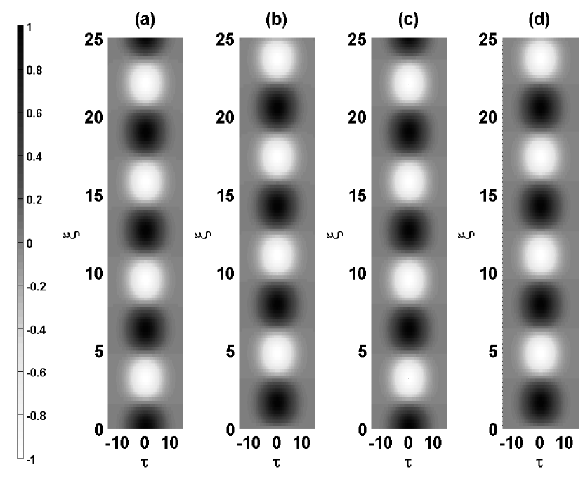
Figure 1: The field evolution in a broad SP pair, with $K_{0}=1$, $T_{0}^{2}=20$. (a,b): The numerical solution of Eq. (2) for $\mathrm{Re}(A_{2}(\xi,\tau))$ and $\mathrm{Im}(A_{1}(\xi,\tau))$, respectively. (c,d): Approximate analytical solution given by Eqs. (5) and (7) for the same components.

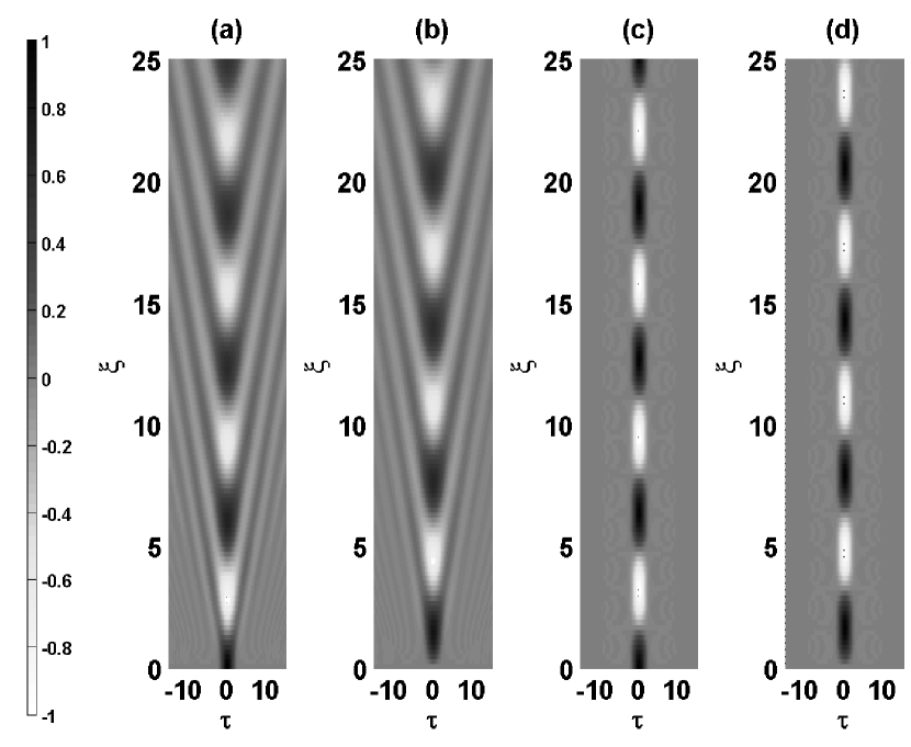
Figure 2: The same as in Fig. 1, but for a narrow SP pair, with $T_{0}=1$.

To analyze the solutions, we define the following correlator between two pairs of functions $\{f_{1}(\xi,\tau),f_{2}(\xi,\tau)\}$ and $\{g_{1}(\xi,\tau),g_{2}(\xi,\tau)\}$:

$$\mathrm{CO}(\{f_{1},f_{2}\},\{g_{1},g_{2}\},\xi)=\frac{|\langle f_{1}|g_{1}\rangle_{\tau}|+|\langle f_{2}|g_{2}\rangle_{\tau}|}{||f_{1}||_{\tau}||g_{1}||_{\tau}+||f_{2}||_{\tau}||g_{2}||_{\tau}},$$ (8)

with the inner product, $\langle f(\xi,\tau)|g(\xi,\tau)\rangle_{\tau}\equiv\int_{-\infty}^{+\infty}{f^{\ast}(\xi,\tau)g(\xi,\tau)d\tau}$, and the corresponding norm, $||f||_{\tau}=\sqrt{\langle f|f\rangle_{\tau}}$. The correlator takes values $0\leq\mathrm{CO}\leq 1$, with $\mathrm{CO}=1$ and $\mathrm{CO}=0$ corresponding, severally, to perfect correlation and no correlation. Then, we can evaluate the proximity of the SP to the periodic behavior as $\mathrm{CO}_{2\pi/K_{0}}=\mathrm{CO}(\{A_{1}(\xi,\tau),A_{2}(\xi,\tau)\},\{A_{1}(\xi+2\pi/K_{0},\tau),A_{2}(\xi+2\pi/K_{0},\tau)\})$, and the consistency between approximate analytical and numerical solutions: $\mathrm{CO}_{\mathrm{AN}}=\mathrm{CO}(\{A_{1\mathrm{N}},A_{2\mathrm{N}}\},\{A_{1\mathrm{A}},A_{2\mathrm{A}}\})$. In particular, as shown in Fig. 3(a), the latter correlator allows one to assess how long the approximate solution remains valid. Naturally, the correlations decay with the increase of $\xi$ and decrease of $T_{0}$. The inset shows the value of the propagation distance, $\xi$, at which $\mathrm{CO}_{\mathrm{AN}}$ drops to $0.95$, as a function $T_{0}^{-2}$, which demonstrates an exponential decrease of the propagation range, in which the analytical solution is valid, with the decrease of the SP’s width.

Further, in Fig. 3(b) the $\mathrm{CO}_{2\pi/K_{0}}$ correlator shows how well the SP pair maintains a periodic evolution pattern. Increasing $T_{0}^{-2}$ causes a parabolic decrease in the correlation, while the degree of the deviation from the perfectly periodic behavior is itself periodic in $\xi$, oscillating at the double frequency, $2K_{0}$.

Figure 3: Correlators computed in the linear system. (a) $\mathrm{CO}_{\mathrm{AN}}(\xi)$ for different temporal widths $T_{0}$ of the SP input. The inset: $\xi(\mathrm{CO}_{\mathrm{AN}}=0.95)$ vs. $T_{0}^{-2}$, the continuous line showing a fit to an exponential function. (b) $\mathrm{CO}_{2\pi/K_{0}}(\xi)$ for different $T_{0}$. The inset: $\mathrm{CO}_{2\pi/K_{0}}(\xi=0)$ vs. $T_{0}^{-2}$, the continuous line showing a fit to a parabola.

The nonlinear system. It is straightforward  to add Kerr terms to the CPEs (2) [25, 20, 28]:

$$\frac{\partial A_{j}}{\partial\xi}-\frac{i}{2}(-1)^{j}\frac{\partial^{2}A_{j}}{\partial\ \tau^{2}}=iK_{0}A_{3-j}+i\Gamma|A_{j}|^{2}A_{j},$$ (9)

where $\Gamma$ is the scaled nonlinearity coefficient. Accordingly, the Lagrangian density (3) acquires an extra term, $\left(\Gamma/2\right)|\left(A_{1}|^{4}+|A_{2}|^{4}\right)$, and the VA can be applied to the nonlinear system as well [27, 26, 28], again assuming $T_{0}\gg 1/K_{0}$. Using the same ansatz (5) as above leads to a nonlinear Schrödinger (NLS) equation featuring a combination of DM with $\bar{\beta}=0$ [cf. Eq. (6)] and nonlinearity management:

$$iA_{\xi}+(1/2)A_{\tau\tau}\cos(2K_{0}\xi)+(\Gamma/4)\left[\cos(4K_{0}\xi)+3\right]|A|^{2}A=0.$$ (10)

This equation can readily produce DM solitons solutions, by dint of methods elaborated in the analysis of the DM and nonlinearity-managed systems [13]-[16].

Comparing numerical solutions produced by Eq. (10) with numerical solutions for the SP pairs produced by simulations of the full system (9) demonstrate that the strong nonlinearity tends to gradually destroy the solitons. In Fig. 4 we display two representative cases for $T_{0}=20$ and $T_{0}=1$ with $\Gamma=0.1$. Only the evolution of $\mathrm{Re}\{A_{2}\}$ is shown, as it is sufficient to represent the situation. The nonlinearity starts to affect the SP shape at propagation distances exceeding the nonlinearity length, $\sim 1/\Gamma=10$. Similar to the linear system (cf. Figs. 1 and 2), the VA, i.e., Eq. (10), is accurate for broad solitons, and inaccurate for narrow ones. The gradual destruction of the SP by the nonlinearity is naturally explained by the fact that, while the fundamental frequency of its internal oscillations falls into the gap [see Eq. (4)], higher-order harmonics, generated by the cubic nonlinearity, couple to the continuous spectrum, initiating decay of the SP.

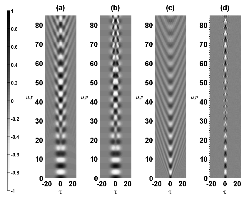
Figure 4: The evolution of the $\mathrm{Re}\{A_{2}\}$ field in the nonlinear system with $\Gamma=0.1$ for a broad SP with $T_{0}=20$: (a) a numerical solution of the full system (9); (b) simulations of the VA-produced single NLS equation (10). (c,d): The same as in (a,b), but for a narrow SP with $T_{0}=1$.

To explore the effect of the nonlinearity in a systematic way, we computed the correlator $\mathrm{CO}_{2\pi/K_{0}}$, using the numerical solutions of the full system (9). The results, shown in Fig. 5, make it evident that stronger nonlinearity worsens the stability of the SP pair. It is worthy to note too that narrower pulses, with smaller $T_{0}$, are more robust against the action of the nonlinearity, which is explained by the similarity of the narrow SPs to the DM solitons, as well as to stationary gap soliton, which exist in the same system [22].

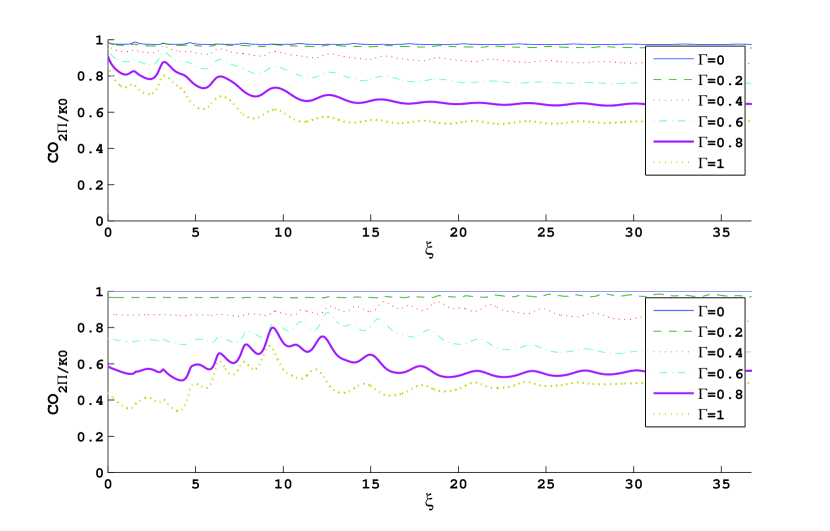
Figure 5: Correlator $\mathrm{CO}_{2\pi/K_{0}}$, characterizing the proximity of the SP pair to a periodically oscillating mode, for different strengths of nonlinearity. The top and bottom panels pertain to narrow and broad pulses, with $T_{0}=2.5$ and $T_{0}=20$, respectively.

Conclusions. We have demonstrated that robust periodically breathing SP (solitary-pulse) pairs can be constructed by linearly coupling two modes with opposite GVD coefficients. In the linear system, a virtually exact analytical solution is found by means of the VA for broad pulses, near edges of the spectral gap. This solution is formally identical to one in the DM model. The VA works well for broad SPs in the nonlinear system as well, reducing the coupled NLS equations to a single one, which includes both the DM and nonlinearity management. Strong nonlinearity tends to destabilize the periodic oscillatory dynamics, although narrower solitons may be sufficiently robust in the nonlinear system. It may be interesting to extend the analysis for higher-order modes, such as dipole SPs.

References

- [1] D. Arbel and M. Orenstein, IEEE J. Quant. Elect. 35, 977-982 (1999).
- [2] D. Turaev, A. G. Vladimirov, and S. Zelik, Phys. Rev. E 75, 045601 (2007).
- [3] C. R. Menyuk, J. K. Wahlstrand, J. Willits, R. P. Smith, T. R. Schibli, and S. T. Cundiff , Opt. Exp. 15, 6677-6689 (2007).
- [4] F. Biancalana, A. Amann, A. V. Uskov, and E. P. O’Reilly, Phys. Rev. E75, 046607 (2007).
- [5] A. B Shvartsburg, Physics-Uspekhi 48, 797 (2005).
- [6] A. Bahabad, M. M. Murnane, and H. C. Kapteyn, Nat Photon 4, 570-575 (2010).
- [7] S. Kobtsev, S. Kukarin, S. Smirnov, S. Turitsyn, and A. Latkin, Opt. Exp. 17, 20707-20713 (2009).
- [8] D. Y. Tang, L. M. Zhao, X. Wu, and H. Zhang, Phys. Rev. A 80, 0236806 (2009).
- [9] A. Zavyalov, R. Iliew, O. Egorov, and F. Lederer, Phys. Rev. A 80, 043829 (2009).
- [10] R. Weill, A. Bekker, V. Smulakovsky, B. Fischer, and O. Gat, Phys. Rev. A 83, 043831 (2011).
- [11] Y. F. Song, L. Li, H. Zhang, D. Y. Shen, D. Y. Tang, and K. P. Loh, Opt. Exp. 21, 10010-10018 (2013).
- [12] J. N. Kutz, SIAM Review 48, 629-678 (2006).
- [13] B. A. Malomed, Soliton Management in Periodic Systems (Springer: New York, 2006).
- [14] S. K. Turitsyn, B. G. Bale, and M. P. Fedoruk, , Phys. Rep. 521, 135-203 (2012).
- [15] R. Ganapathy, Commun. Nonlin. Sci. Numer. Simul. 17, 4544-4550 (2012).
- [16] Y. V. Kartashov, B. A. Malomed, and L. Torner, Rev. Mod. Phys. 83, 247-306 (2011).
- [17] J. Scheuer and M. Orenstein, J.Opt. Soc. Am. B 19, 732-739 (2002).
- [18] T. C. Hernandez, V. E. Villargan, V. N. Serkin, G. M. Aguero, T. L. Belyaeva, M. R. Peña, and L. L. Morales, Quant. Electr. 35, 778-786 (2005).
- [19] M. J. Ablowitz and J. F. Ladik, J. Math. Phys. 17, 1976.
- [20] A. Yariv and P. Yeh. Photonics: Optical Electronics in Modern Communication (Oxford University Press: Oxford, 2007).
- [21] A. D. Boardman and K. Xie, Phys. Rev. A 50 1851-1866 (1994).
- [22] D. J. Kaup and B. A. Malomed, J. Opt. Soc. Am. B 15, 2838-2846 (1998).
- [23] S. Arismar Cerqueira, Jr. , Rep. Prog. Phys. 73, 024401 (2010).
- [24] B. Dana, L. Lobachinsky, and A. Bahabad, (to be published).
- [25] G. Agrawal. Applications of Nonlinear Fiber Optics (Elsevier: 2010).
- [26] C. Paré and M. Florjańczyk, Phys. Rev. A 41, 6287-6295 (1990).
- [27] P. L. Chu, B. A. Malomed, and G. D. Peng, , J. Opt. Soc. Am. B 10, 1379-1385 (1993).
- [28] Q. Li, Y. Xie, Y. Zhu, and S. Qian, Opt. Commun. 281, 2811-2818 (2008).