Influence of system size on the properties of a fluid adsorbed in a nanopore: Physical manifestations and methodological consequences

Abstract

We consider the theoretical description of a fluid adsorbed in a nanopore. Hysteresis and discontinuities in the isotherms in general hampers the determination of equilibrium thermodynamic properties, even in computer simulations. A proposed way around this has been to consider both a reservoir of small size and a pore of small extent in order to restrict the fluctuations of density and approach a classical van der Waals loop. We assess this suggestion by thoroughly studying through density functional theory and Monte Carlo simulations the influence of system size on the equilibrium configurations of the adsorbed fluid and on the resulting isotherms. We stress the importance of pore-symmetry-breaking states that even for modest pore sizes lead to discontinuous isotherms and we discuss the physical relevance of these states and the methodological consequences for computing thermodynamic quantities.

I Introduction

Phase equilibria and transitions in confined fluids have attracted wide interest over the years among theorists and experimentalists. A ubiquitous feature of these systems is the appearance of a reproducible hysteresis loop in the adsorption and desorption isotherms. More generally, a variety of intermediate states may be visited by the fluid, depending on the characteristics of the experimental setup. The thermodynamic analysis of these states can be quite involved due to the irreversibility which prevents using standard methods such as thermodynamic integration. Several techniques have therefore been devised to calculate equilibrium properties such as the free energy, which is of primary importance to determine true equilibrium states and limits of metastability, or the critical nucleus for condensation in the framework of the classical nucleation theory. Some years ago, Neimark and coworkersneimark (02) proposed the “gauge-cell method” which is based on the construction of a continuous isothermal trajectory of equilibrium states in the form of a van der Waals loop. The unstable states, which cannot be obtained in grand-canonical simulations of large systems in the thermodynamic limit, are then supposed to be stabilized by suppressing the density fluctuations in the system. This could be done by reducing both the reservoir size (which limits the fluctuations of the mean density by approaching the canonical condition) and the system size (which limits the local variations of density in space), which then amounts to considering a “mesoscopic canonical ensemble”. Provided that a continuous isotherm is obtained, equilibrium thermodynamic functions can then be determined by thermodynamic integration along the metastable and unstable regions.neimark (02)

In our previous work,puibasset (09) we studied by simulations in the mesoscopic canonical ensemble the influence of the reservoir size on the path followed by a simple fluid adsorbed in a nanopore of ideal geometry (a slit) during adsorption and desorption. We found states of intermediate density between the gas-like and liquid-like branches. The intermediate states break the symmetry of the slit-pore geometry in one direction, taking the morphology of liquid bridges (or “rails”), gas bubbles (or gas “cylinders”) and of undulations or bumps of the liquid layers. These states are “conditionally stable”, as they are stabilized by the constraint of fixed total number of particles in the pore-plus-reservoir system, but we showed that they are neither stable nor metastable under grand-canonical conditions. (This is quite different from the situation encountered in disordered porous materials where the system under a strict canonical or a mesoscopic canonical constraint passes through states that are grand-canonically metastable.kierlik (09)) We also found that discontinuities, which correspond to “morphological transitions” between different types of intermediate states, remain in the isotherms even for small reservoir sizes when the isotherms become reversible.

The present paper extends our previous study by investigating the effect of the system size, defined as the size of the simulation cell comprising the pore of slit or cylinder geometry, on the spatial variations of the density profile. We also analyze the robustness of the thermodynamic integration method. We consider a small (or even vanishingly small) reservoir, which ensures an almost canonical ensemble setting, as used in the gauge-cell method. We address the following theoretical and methodological questions:

(1) Are there conditions and system sizes for which the isotherms have the form of a continuous van der Waals-like loop?

As already mentioned, suppressing the density fluctuations is the key: a van der Waals loop is typically obtained in mean-field approximations when density fluctuations are completely neglected. In the presence of an external potential, as in the present case of a fluid in a slit- or cylinder-shaped pore, this amounts to considering a mean density profile that retains the spatial symmetry of the pore: $\rho(z)$, with $z$ the axis perpendicular to the parallel walls in a slit pore, or $\rho(r)$, with $r$ the radial coordinate in the cross-section for a cylindrical pore. Calculations of this kind can be performed within mean-field density functional theory which has become a standard tool in the field of adsorption.

What happens when one lifts the symmetry requirement on the density profile and allows profiles that break the pore symmetry? We answer this question by investigating the behavior of an adsorbed fluid both by density functional theory for a coarse-grained lattice-gas model and by Monte Carlo simulations of an atomic model in conditions equal or close to a canonical-ensemble setting. The density-functional theoretical study shows, as somewhat anticipated, that for a system size reduced to one lattice spacing in the two directions parallel to the slit walls (with periodic boundary conditions), one indeed recovers a mean density profile $\rho(z)$ and a continuous van der Waals loop. However, when the system size is increased, symmetry-breaking density profiles, of the form $\rho(x,z)$ and $\rho(x,y,z)$, appear as equilibrium solutions for certain regions of the isotherms. These spatially nonsymmetric solutions appear for modest system sizes and their presence gives rise to morphological transitions and discontinuities in the fluid isotherms. A similar phenomenon is observed in the Monte Carlo simulation of an atomic fluid in slit and cylinder pores, for which discontinuities associated with morphological transitions appear in the isotherms for system sizes of the order of the pore width or diameter.

(2) What is the physical meaning of the intermediate, symmetry-breaking states obtained for finite system sizes?

In the thermodynamic limit, all intermediate states should disappear from thermodynamic functions and observables as their free-energy is always higher than that of the main gas-like and liquid-like branches due to the cost of the additional interfaces involved. Nevertheless, they can still be relevant to describe effects that are subdominant to the bulk ones. In particular, one can take advantage of the stabilization of symmetry-breaking states and density profiles by finite system sizes (in the canonical ensemble) to extract the properties of the interfaces, among which the liquid-gas surface tension in the adsorbed fluid. We illustrate this for the density-functional calculation and the Monte Carlo simulation. Even one step further, some symmetry-breaking states serve as proxies for determining the characteristic nucleus for condensation in a pore and estimating the associated free-energy barriers.

(3) Is thermodynamic integration doomed to failure when discontinuities associated with morphological transitions are present in the isotherms?

We have found (see above) that discontinuities in the equilibrium isotherms appear for quite modest system sizes. In realistic models, smaller system sizes do lead to continuous isotherms, but the finite-size effects on the properties of the system are so large that one cannot hope to describe the thermodynamic limit in this way. The window of system sizes for which the isotherms are continuous but the thermodynamic properties are already those of the macroscopic system is therefore extremely small if not inexistent. This may seem as a serious drawback for thermodynamic integration. However, we have found that there is a significant range of system sizes that do not lead to observable finite-size effects on the thermodynamic properties and that still allow equilibration of the adsorbed fluid so that the isotherms are reversible (recall that hysteresis effects seem almost unavoidable both numerically and experimentally in large to macroscopic systems). For such sizes, the isotherms are discontinuous but the discontinuities can be handled as some thermodynamic functions are still continuous across these discontinuities. We show that this is the case for Monte Carlo simulations of an adsorbed atomic fluid in a mesoscopic canonical ensemble, and this suggests that thermodynamic integration then remains a practical tool provided one appropriately chooses the system sizes on which to apply it.

The paper is organized as follows. In section II, we introduce the setup and the model, and we describe the algorithms used in the DFT calculations and the simulation method. For the former, we have devised a way to obtain solutions for the density profiles that break the pore symmetry, in a canonical ensemble. In section III we discuss the influence of the system size on the states visited by the fluid at equilibrium. A detailed analysis of the domain of existence of these states and of the associated symmetry-breaking density profiles is given for the DFT results. For the MC simulations, we focus on the validity of the thermodynamic-integration method in the mesoscopic canonical ensemble. Finally, we conclude in section IV.

II Model and Methods

We consider a fluid adsorbed in a pore of ideal geometry in setups corresponding to different thermodynamic ensembles: grand-canonical, canonical, and a mixed ensemble called the mesoscopic canonical ensemble.pana (87); smit (89, 89b) The latter is extensively used in the gauge cell method introduced by Neimark and coworkers.neimark (00, 05, 05b, 05c); vishny (03) In this ensemble, the pore is in contact with a reservoir of finite (possibly small) relative size. The cross section of the pore is fixed, while its length may be changed in order to study its influence on the adsorption/desorption measurements.

In this work, we use two complementary methods: the density-functional theory (DFT) on a coarse-grained lattice-gas model and Monte Carlo (MC) simulations of an atomic fluid. The former allows us to explore a large domain of system sizes and to have an easy access to thermodynamic information, such as the fluid grand potential. The later on the other hand provides a clear interpretation of the results in terms of molecular configurations.

II.1 Density Functional Theory

As discussed in previous papers,kierlik (02); detcheverry (03) our DFT description is based on a coarse-grained lattice-gas model. We consider a fluid on a simple cubic lattice that is confined in a slit pore of fixed width $H$ in the $z$ direction, with periodic boundary conditions applied in the $x$ and $y$ directions parallel to the slit walls. Multiple occupancy of a site is forbidden and only nearest-neighbor interactions are taken into account. The starting point of our theoretical analysis is the following expression of the free-energy functional in the local mean-field approximation:

$$F[\{\rho_{i}\}]= k_{B}T\sum_{i}[\rho_{i}\ln\rho_{i}+(1-\rho_{i})\ln(1-\rho_{i})]$$ (1)

$$-w_{ff}\sum_{<ij>}\rho_{i}\rho_{j}-\sum_{i}\rho_{i}\phi_{i},$$

where $\rho_{i}$ and $\phi_{i}$ are, respectively, the thermally averaged fluid density and the (attractive) external field at site $i$; $w_{ff}$ denotes the fluid-fluid attractive interaction and the double summation runs over all distinct pairs of nearest-neighbor sites. In our case, $\phi_{i}=0$ everywhere except for sites near the pore walls where $\phi_{i}=w_{sf}$, the solid-fluid attractive interaction.

To get a reference, we first start with the grand canonical situation where fluid particles can equilibrate with an infinite reservoir that fixes the chemical potential $\mu$. Minimizing the grand-potential functional $\Omega[\{\rho_{i}\}]=F[\{\rho_{i}\}]-\mu\sum_{i}\rho_{i}$ with respect to $\{\rho_{i}\}$ at fixed $T$ and $\mu$ yields a set of coupled equations,

$$\rho_{i}=\frac{1}{1+\exp[-\beta(\mu+w_{ff}\sum_{j/i}\rho_{j}+\phi_{i})]},$$ (2)

where the sum $\sum_{j/i}$ runs over the $c=6$ nearest neighbors of site $i$. By using a simple iterative method to solve these equations, one finds solutions that are only minima of the grand potential surface, i.e. metastable states. The adsorption isotherm is obtained by increasing the chemical potential in small steps $\delta\mu$. At each subsequent $\mu$, the converged solution at $\mu-\delta\mu$ is used to start the iterations.

We next study the canonical ensemble, i.e. when the total number $N=\sum_{i}\rho_{i}$ of the fluid particles is fixed. The isotherm is then obtained by increasing $N$ in small steps $\delta N$. In this case, the system tries to minimize its Helmholtz free-energy $F$. This can be solved by the method of Lagrange multipliers. We consider the function

$$\bar{F}[\{\rho_{i}\},\lambda,T]=F[\{\rho_{i}\},T]+\lambda\{N-\sum_{i}\rho_{i}\},$$ (3)

where $\lambda$ is a Lagrange multiplier that has the meaning of a chemical potential coupled to the local densities. Minimizing $F$ with the constraint on the local densities amounts to simultaneously solving the coupled equations $\frac{\partial\bar{F}}{\partial\rho_{i}}=0$ and $\frac{\partial\bar{F}}{\partial\lambda}=0$, or equivalently,

$$k_{B}T\ln[\frac{\rho_{i}}{1-\rho_{i}}]-\lambda-w_{ff}\sum_{j/i}\rho_{j}-\phi_{i}=0,\quad 1\leq i\leq V$$

$$N-\sum_{i}\rho_{i}=0$$ (4)

where $V$ is the total number of sites. One has then to define an iterative scheme that specifies how the system goes from one converged solution to another as the total number of particles is slowly changed. The details were given in a previous paper.kierlik (09) If the algorithm converges, it does not necessarily converge to a local minimum, nor even to an extremum, as the constraint can stabilize an unstable state (stable or unstable refers here to the grand-canonical situation). As illustrated below, we indeed find physically acceptable configurations for the local densities ${\rho_{i}}$, which are nonetheless unstable in the grand-canonical ensemble (a condensation nucleus for instance).

One knows from a previous studyMaier (01) that the solution space of the DFT in the canonical ensemble for an infinite slit pore can be very complex. We are not interested here in finding all solutions to the system of coupled non-linear equations in Eq. (II.1) but rather in understanding the physical states that typically appear along the adsorption path followed by the system when changing the system size. We have therefore performed calculations by varying the lateral dimensions $L$ (length) along the $x$-axis and $\ell$ (width) along the $y$-axis and applying periodic boundary conditions in both directions.

(1) As already mentioned in the introduction, the case $L=l=1$ corresponds to configurations with a uniform density inside a given layer, i.e. to a density profile $\rho(z)$ that is invariant along $x$ and $y$ axes. The canonical isotherm should be continuous and reversible, which allows safe thermodynamic integration as for the usual van der Waals loop for homogeneous vapor-liquid phase transition.

(2) We then increase the length $L$ (keeping $\ell=1$) and search for solutions $\rho(x,z)$ that can break the spatial symmetry along the $x$-axis. However, since the DFT does not account for thermal fluctuations, the symmetry cannot be spontaneously broken with a simple iterative method. To remedy this, we temporarily modify the external potential by increasing (resp. decreasing), in the case of adsorption (resp. desorption), its value by a few percents for one site in each of the layers adjacent to the walls ($z=1$ and $z=H$). When convergence has been reached with the modified potential, we switch back to the original potential and restart the iteration process with the previously converged solution. With this procedure, one checks whether a symmetry-breaking solution can persist with a symmetric potential and therefore appears as an equilibrium solution in the canonical ensemble.

(3) Finally, we search for solutions $\rho(x,y,z)$ by varying both $L$ and $\ell$. We use the same methodology as before to promote symmetry breaking solutions: we temporarily modify the external potential on a rectangular array of sites in the layers close to the walls, which favors the appearance of liquid bridges or vapor bubbles. We choose a rectangle with dimensions $L/4\times\ell/4$ because we observed that a modification on a too small array of sites does not allow the solution to break the symmetry. We also systematically checked the stability of the solutions so obtained when reverting to the unperturbed symmetric potential.

Generically, the isotherms obtained from the above solutions display a hysteresis between adsorption and desorption. As extensively documented, hysteresis is ubiquitous in adsorption/desorption phenomena. It appears as a consequence of very long equilibration times associated with high free-energy barriers. However, the hysteresis found in the DFT description of adsorbed fluids is rather an artefact of the mean-field approximation that suppresses the thermal fluctuations and does not allow the system to overcome any energy barrier, whatever its magnitude. In the present problem, this represents an obstacle as we are interested in small system sizes for which equilibration should not be a problem in any realistic system. Actually, we find in the Monte Carlo simulations that equilibration does take place for the system sizes studied. To get around this problem, we have taken advantage of the fact that the free energy of the solutions is easily computed from Eq. (1) to look for the solutions with minimal free energy. The latter should then represent the equilibrium states and describe a reversible isotherm.

II.2 Monte Carlo simulations

The objective is to build the adsorption/desorption isotherms of a simple fluid in a porous material in equilibrium with a finite reservoir. In this work, the reservoir is chosen as small as possible, so that the statistical ensemble is essentially canonical. The reservoir is used as a tool to introduce or remove fluid in the system through favorable insertions, in order to build the isotherms. In our systems, the ratio between the reservoir size and the pore size is 66.7 for the slit pore and 50 for the cylinder. Due to the large difference in densities between the condensed fluid and the gas phase in the reservoir, essentially all atoms are then in the pore.

The system and the reservoir are both in thermal equilibrium (imposed temperature) and in chemical equilibrium. The chemical equilibrium is achieved by particle exchange, the total number of particles being constant. In order to obtain the adsorption isotherm, the total number of particles is increased stepwise. The extra particles are introduced in the reservoir, and, after a while, the system equilibrates, resulting in a new chemical potential $\mu$ for the system, and a new average density of particles $\rho(\mu)$ in the pore. After complete filling of the system, the desorption isotherm is obtained by decreasing in a similar way the total number of particles. Using various amounts of particles for addition or removal of the fluid in the system produces identical isotherms, with more or less points along it. A compromise is thus chosen between precision and computing time. In some cases to be described later, the adsorption/desorption isotherms may exhibit discontinuities or gaps. In such situations, we have decreased the particle increment around the discontinuities to improve the accuracy.

The numerical resolution is performed by Monte Carlo simulation using the Metropolis algorithm for particle displacements (thermalization) and particle exchange between the porous material and the reservoir (chemical equilibration). The pore geometry (slit or cylinder) and the (monoatomic) fluid are chosen to capture the main features of fluid states in pores of simple geometry. The system mimics argon adsorption in nanoporous solid carbon dioxide. The interactions are modeled by Lennard-Jones potentials, which are truncated at three atomic diameters for convenience. The parameters describing the fluid-fluid interactions are those for argon ($\epsilon_{\rm ff}/k_{B}=119.8$ K and $\sigma_{\rm ff}=0.3405$ nm), while the fluid-wall parameters are $\epsilon_{\rm fw}/k_{B}=153.0$ K and $\sigma_{\rm fw}=0.3725$ nm.puibasset (05, 05b) All thermodynamic quantities are normalized by the fluid-fluid Lennard-Jones interaction parameters. The wall roughness of the pores is neglected, and the fluid-wall potential is obtained by integrating the Lennard-Jones potential over a uniform density of interacting sites.

Two pore geometries are considered. A slit pore of given height $H=6$ (in units of the fluid atomic diameter) and dimensions parallel to the walls equal to $\ell=8$ in one direction (width) and varying between $L=4$ and $L=40$ in the other direction (length of the pore). Periodic boundary conditions are applied in the two directions parallel to the walls. The cylindrical pore is of fixed diameter $D=6$, the length varying between $L=4$ and $L=24$. Periodic boundary conditions are applied along the cylinder axis. It has been checked that the gas in the reservoir is always ideal in this study, and thus need not to be treated explicitly, which speeds up the calculations.

In order to discuss notions such as stability, coexistence and nucleation in the mesoscopic canonical ensemble, one has to calculate thermodynamic potentials. The whole pore-plus-reservoir system being in the canonical ensemble, the total Helmholtz free energy is the quantity of interest. For a small reservoir (quasi-canonical situation), this total free energy is close to the Helmholtz free energy of the fluid confined in the pore. On the other hand, if the reservoir is large enough, the pore is almost in the grand-canonical ensemble, and one is then interested in the calculation of the grand potential. The grand potential is also useful to check whether the (inhomogeneous) intermediate fluid states observed in the mesoscopic canonical ensemble are metastable in the grand canonical ensemble.puibasset (09) The grand-potential density may be evaluated either directly during the course of the simulation or by thermodynamic integration along the adsorption isotherm. The corresponding algorithms are presented now.

In our previous workkierlik (09); puibasset (09) we showed that the chemical potential, when defined in each part of the system (pore and reservoir) by using Widom’s insertion method or the ideal approximation in the reservoir, exactly coincides with the rigorous definition derived from the canonical ensemble for the complete system. Similarly, a thermodynamic pressure (denoted $\Pi_{\rm P}$), equal to minus the grand-potential density, may be defined in the pore as the conjugate quantity to the pore dimension $L$ parallel to the walls. This quantity is calculated numerically during the course of the simulation by using the virtual-volume-variation methodeppenga (84); harismiadis (96); vortler (00) according to

$$\Pi_{\rm P}=\Pi_{\rm P}^{\rm id}+\Pi_{\rm P}^{\rm ex}=k_{B}T\frac{\left<N\right>}{\mathcal{A}L}+\frac{1}{\mathcal{A}}\left<{\frac{\delta U}{\delta L}}\right>{\rm,}$$ (5)

where $\Pi_{\rm P}^{\rm id}$ and $\Pi_{\rm P}^{\rm ex}$ are the ideal and excess contributions to the grand-potential density, $\mathcal{A}$ is the cross-section area (equal to $H\ell$ for the slit pore, and $\pi D^{2}/4$ for the cylinder), $U$ is the configuration energy of the fluid confined in the pore, $\delta U$ its variation associated with the virtual variation $\delta L$ (in this case, a homogeneous stretching parallel to the pore length $L$), and the brackets denote the statistical average over Monte Carlo configurations. Note that the virtual changes do not interfere with the Markov chain generation, i.e. they are not Monte Carlo trials to be accepted or rejected to generate new configurations.

It should be stressed that Eq. (5) holds only if the fluid is homogeneous in the direction where the virtual variations are performed. The method can thus never be applied along the radial direction for the cylindrical pore, or perpendicular to the walls for the slit pore. The most favorable direction is along the pore length $L$ (pore symmetry). However, as shown later, the fluid profiles may break the pore symmetry: in this case the virtual-volume-variation method fails. In the particular case of the slit pore, due to the symmetry between the $\ell$ and $L$ directions, the virtual-volume-variation method can also be performed along the direction $\ell$. This property can be used to calculate the grand-potential density in the situations where the fluid profile break the pore symmetry along $L$ while it remains homogeneous along the $\ell$ direction.

The Helmholtz free energy $F$ of the pore-plus-reservoir system can be calculated by integrating the relation

$$\left.\frac{\partial F(N,V,T)}{\partial N}\right|_{V,T}=\mu{\rm.}$$ (6)

where $N$ is the total number of particles including the pore and the reservoir. Note that this integration should be restricted to the continuous portions of the isotherms. A portion of an isotherm is qualified as continuous if it is possible to reduce the interval between two successive simulation points by performing extra simulations with smaller increments in the total amount of particles. In this situation, the numerical (discrete) thermodynamic integration of $\mu(N)$ can give the total Helmholtz free energy variations within an uncertainty that can be made as small as wanted by decreasing the increments between successive points (with, of course, the lower limit of one atom).

In principle, this integration cannot be performed over the whole isotherm when the latter exhibits discontinuities. However, when the isotherms are reversible (see below), and therefore presumably at equilibrium, one can use thermodynamic integration even when discontinuities in $\mu(N)$ are present, as the total Helmholtz free energy $F$ and the total number of particles $N$ are the same on both sides of the discontinuities.

The grand potential in the pore is then given by

$$\Omega_{\rm P}=F-\mu N-\Omega_{\rm R}$$ (7)

where $\Omega_{\rm R}$ is the grand potential in the reservoir. As previously mentioned, the gas in the reservoir is close to ideality, and therefore $\Omega_{\rm R}=-k_{B}T\left<N_{\rm R}\right>$, where $\left<N_{\rm R}\right>$ is the average number of particles in the reservoir. The corresponding grand-potential density is $\Pi_{\rm P}=-\Omega_{\rm P}/V_{\rm P}$, where $V_{\rm P}$ is the pore volume.

III Results

III.1 DFT: influence of the system size on the equilibrium density profiles

All the illustrative calculations here are for a pore width $H=6$, a reduced temperature $T^{*}=k_{B}T/w_{ff}=1.0$ and a ratio $w_{sf}/w_{ff}=3$, as already studied in Ref. [monson, 08]. They are performed by assuming the reflection symmetry, $\rho(x,y,z)=\rho(x,y,H-z)$.

III.1.1 Grand-canonical isotherms

The whole adsorption (desorption) grand-canonical (GC) isotherm is obtained by starting from a low (high) chemical potential and increasing (decreasing) the chemical potential in a series of steps, with the solution at each state forming the initial guess for the solution at the next state. Results for the average density are shown in Fig 1. The isotherms exhibit two jumps corresponding, first, to a monolayer formation involving the sites adjacent to each of the pore walls and, second, to a vapor-liquid transition (capillary condensation) for the confined lattice fluid as illustrated in Fig. 1 by sketches of the density distribution. This latter jump is accompanied by a pronounced hysteresis and the equilibrium vapor-liquid transition is determined by the crossing of the adsorption and desorption branches in the $(\mu,\Omega)$ plane. These results are what could be expected for this very simple and ideal system. Note that one never observes inhomogeneous density profiles in the $(x,y)$ plane, even when temporarily breaking the symmetry of the external potential as detailed in section II. More precisely, no coexistence between the vapor-like and the liquid-like phases is observed in the GC ensemble as such coexistence needs an interface and requires additional free-energy cost compared to the homogeneous vapor or liquid states: such states are therefore never minima of the grand potential.

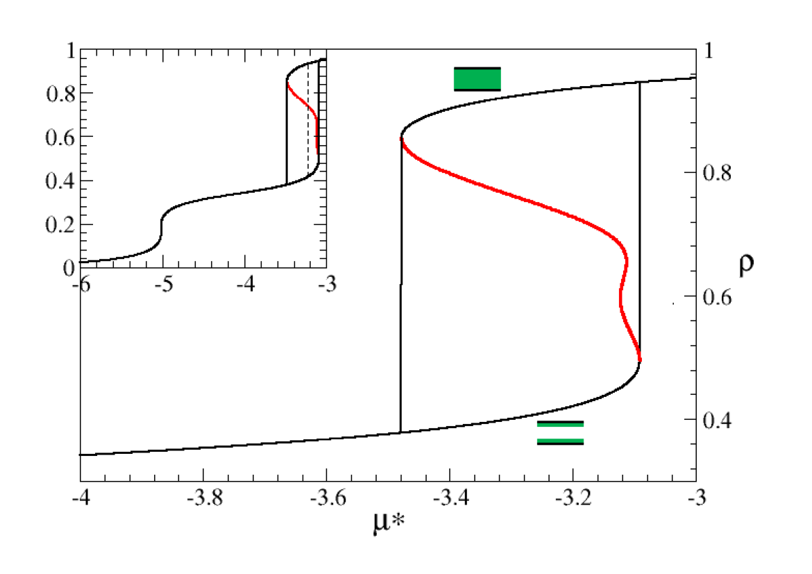
Figure 1: (color on line) DFT adsorption and desorption isotherms for a fluid adsorbed in a slit pore in the grand-canonical (black line with vertical jumps) and canonical (red line) ensembles. The reduced chemical potential $\mu^{*}$ is defined in units of $w_{ff}$. Inset: The whole isotherm. Main panel: The capillary-condensation region. Sketches of the fluid density distribution are also shown.

III.1.2 Evolution of the canonical isotherms varying the size of the system

We are primarily interested in studying the solutions for the fluid in a slit pore under canonical-ensemble [fixed $(N,V,T)$] conditions. In this case, the increment of the average density $\overline{\rho}=\frac{N}{V}$ has been chosen as small as $10^{-4}$ and convergence has been assumed when differences for $\rho$ between two successive iterations is below $10^{-8}$. We describe below three different situations according to the size of the system along the $x$-axis, $L$, and along the $y$-axis, $\ell$.

$L=\ell=1$.

One first begins with solutions of the form $\rho(z)$. As illustrated in Fig. 1, the sequence of states follows the GC isotherm until the end of the adsorption branch. Beyond the GC stability limit of the vapor-like branch, the loop exhibits re-entrance (decreasing $\mu$ with increasing $\overline{\rho}$) until it reaches the GC liquid-like branch. The (expected) continuous $S$-shape of the isotherm shows however a small portion with a positive isothermal compressibility, i.e. $\frac{\partial\overline{\rho}}{\partial\mu}>0$, which is then grand-canonically stable. The other re-entrant states are grand-canonically unstable and are only stabilized by the constraint (closed system of a finite volume). Nevertheless, the consistency of the DFT guarantees that integrating $\mu(N)dN$ between $N_{1}$ and $N_{2}$ gives the differences $F_{2}-F_{1}$ computed from Eq. 1.

$L>1,\ell=1$.

When $L$ remains small, one finds the same solution as for $L=\ell=1$, i.e. the solution that preserves the symmetry of the external potential. Spatial fluctuations in the $x$-direction disappear when one removes the perturbative symmetry-breaking potential. Above $L=6$ however, even if the continuous character of the isotherm is preserved, a large deviation appears in the upper part. Inspection of the density profiles reveals that a symmetry breaking takes place. The density profile is no longer uniform along the $x$-axis and shows a significant undulation outside the first layer in contact with the substrate. The deviation in the hysteresis loop from the $L=1$ case has a local $S$-shape that displays a horizontal jump for $L$ = 8 and above.

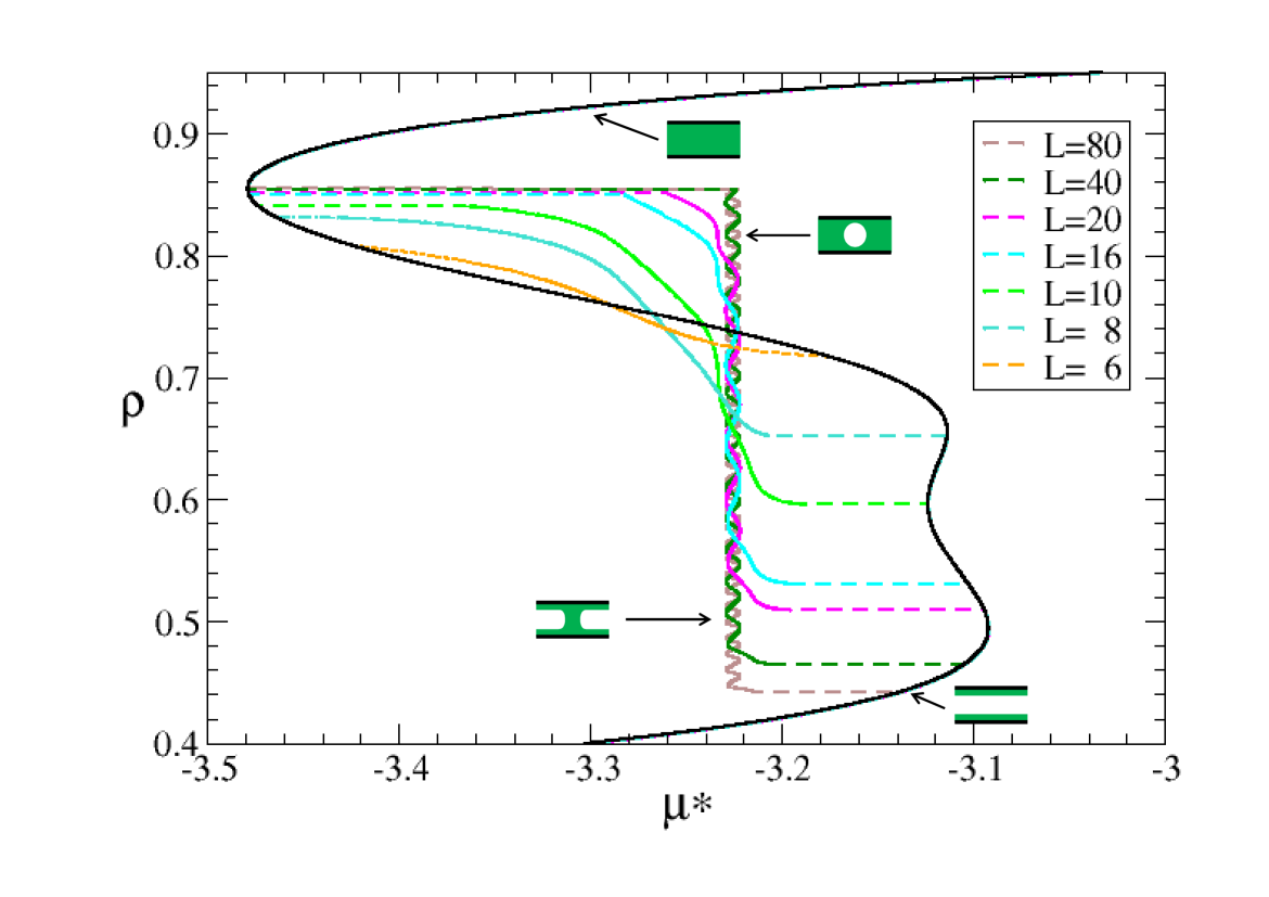
Figure 2: (color on line) DFT canonical desorption isotherms for various lengths $L$ and $\ell=1$. The density is allowed to fluctuate along $x$ and $z$. Sketches of the fluid density distribution are also shown in the $(x,z)$ plane.

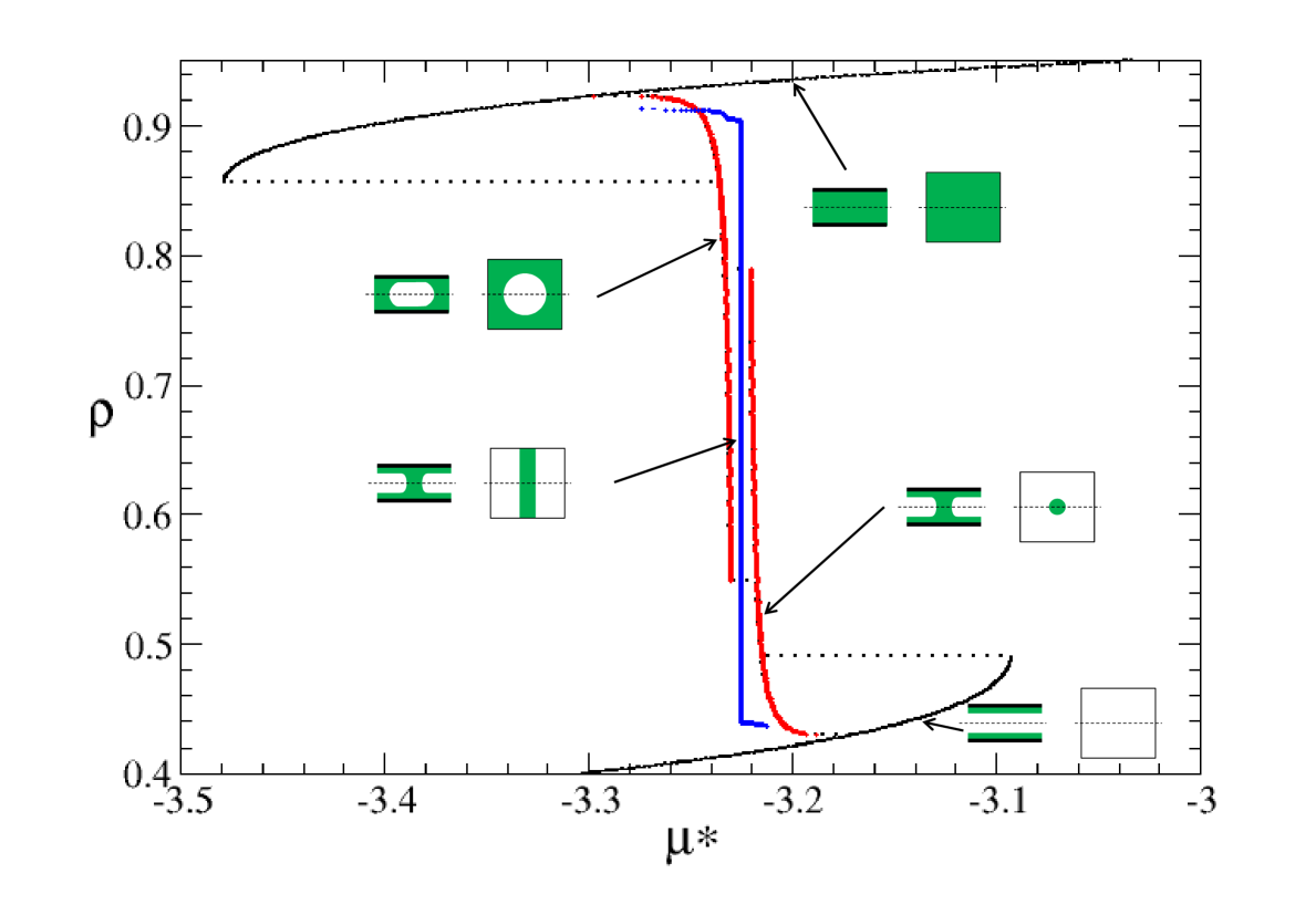
Figure 3: (color on line) Stable and metastable states for $L=\ell=100$, as obtained by DFT in the canonical ensemble. Two “homogeneous” (gas-like and liquid-like phases that satisfy the slit-pore symmetry, shown in black), and three inhomogeneous branches (rail, shown in blue, droplet and bubble, shown in red) are displayed with their whole domains of stability. Sketches of the fluid density distribution are shown both in the $(x,z)$ and $(x,y)$ planes. For clarity, the oscillations of the chemical potential of the rail state around the coexistence value are not displayed and only the average value is plotted.

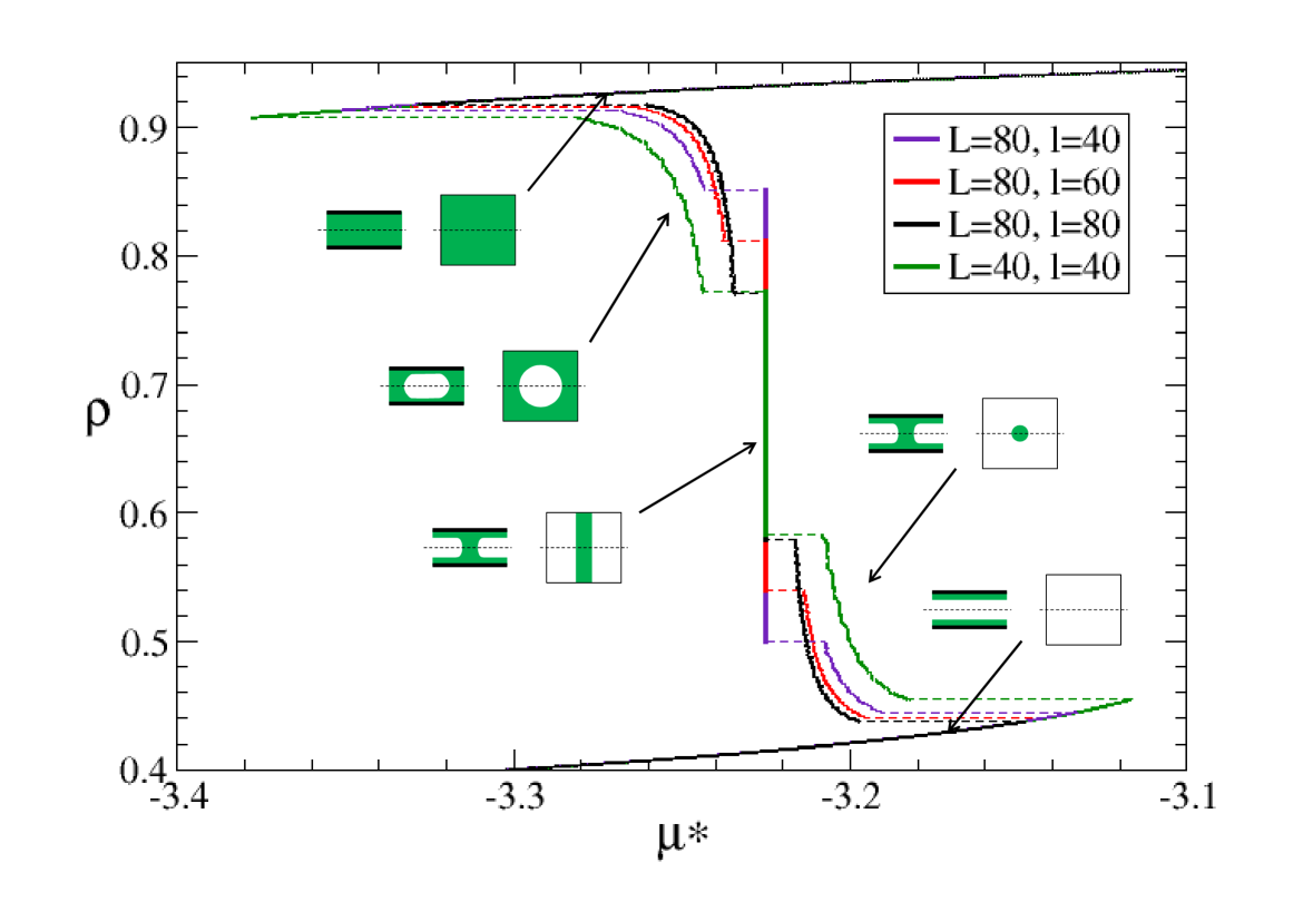
Figure 4: (color on line) Equilibrium states for various system sizes $L$ and $\ell$, as obtained by DFT in the canonical ensemble. Jumps between these branches are the signatures of morphological transitions. Sketches of the fluid density distribution are shown both in the $(x,z)$ and $(x,y)$ planes. For clarity, the oscillations of the chemical potential of the rail state around the coexistence value are not displayed and only the average value is plotted.

This is illustrated in Fig. 2 in the case of the canonical desorption isotherms, where the effects are more pronounced than in the adsorption case. Starting from saturation, all systems, whatever the size (including $L=1$), follow the GC desorption branch until the stability limit of the liquid-like phase on this branch. Below this point, differences appear between the solution $\rho(z)$ (corresponding to $L=1$) and the symmetry-breaking solutions $\rho(x,z)$. The first horizontal jump that leads to a departure from the $L=1$ canonical isotherm takes place for a point in the $(\mu,\rho)$ plane which becomes closer to the stability limit of the upper GC branch as $L$ increases. The system then reaches an inhomogeneous state which, above $L=40$, corresponds to a “rail” of vapor in a liquid environment (assuming the invariance along the $y$-axis). The chemical potential for this rail state corresponds to the liquid/vapor coexistence in the pore, $\mu_{coex}=-3.22$. (The chemical potential actually oscillates around this value, but this is an artifact of the underlying lattice.) This can be understood as follows. The rail of vapor needs a minimum size to be (canonically) stable. To generate this inhomogeneous state, a depletion should be created in the homogeneous (along $x$-axis) liquid phase and the corresponding excess density redistributed in the rest of the system. This becomes easier as the longitudinal system size $L$ increases and for a large $L$ it happens as soon as the GC branch becomes unstable. For smaller values of $L$ the presence of some extensions that stick out of the liquid-vapor vertical coexistence line reflects the fact that the hole has not yet reached its canonically stable shape and is deformed.

The same type of behavior occurs for the second jump in the desorption isotherm, from a rail of liquid in a vapor environment to the lower (vapor-like) GC branch. As discussed in a previous paper,puibasset (09) this second jump should disappear in the thermodynamic limit as the system would then follow the liquid-vapor coexistence line down to the GC branch. For the canonical adsorption isotherms (not shown), the phenomena are reversed: for large systems, the first jump links the end of the lower GC branch to the liquid-vapor coexistence line and the second jump gets closer and closer to the upper (liquid-like) GC branch as the system size increases until it vanishes in the thermodynamic limit.

$L>1,\ell>1$.

Increasing the size of the simulation box in both lateral directions and allowing fluctuations along the $y$-axis in addition to those along the $x$-axis reveals the existence of other inhomogeneous metastable states. This is illustrated in Fig. 3 for the largest system ($L=100,\ell=100$) that we have studied. The two separate branches on each side of the liquid-vapor coexistence line are reached by the fluid when the homogeneous states become unstable to the introduction of the rectangular symmetry-breaking perturbative potential. Upon adsorption (resp. desorption), the inhomogeneous state reached by the system corresponds to a liquid droplet (resp. vapor bubble) bridging the two surfaces of the slit pore in a vapor (resp. liquid) environment. This is easily seen by visual inspection of the density profiles. The system does not spontaneously reach the rail state, as discussed below, and the droplet (resp. bubble) branch extends until its stability limit. However, this kind of behavior is not generic: for smaller values of $\ell$, the adsorption (resp. desorption) isotherm jumps from the droplet (resp. bubble) to the rail state and a second jump to the upper (resp. lower) GC branch next takes place.

III.1.3 Morphological transitions and interfacial properties

Searching for symmetry-breaking density profiles in systems of increasing size has revealed the existence of inhomogeneous states. Jumps take place between these states and the gas-like and liquid-like states, but not at equilibrium. Instead, a large hysteresis is observed when varying the mean density, which corresponds to the “superspinodals” found in Ref. [neimark, 00]. To get rid of this spurious hysteresis (see the discussion at the end of II.A), we have computed the equilibrium canonical isotherm for a given system size by finding the minimum of the Helmholtz free energy among all identified states : the two symmetric liquid-like and vapor-like (upper and lower GC branches) and the three inhomogeneous (rail, droplet and bubble branches) states. The jumps in the chemical potential between these equilibrium branches correspond to “morphological transitions”, i.e. a sudden spatial redistribution of the density profile inside the pore at a fixed mean density. Results are shown in Fig. 4 for various system sizes ($L\times\ell=40\times 40,80\times 80,100\times 100$, and $80\times 40$).

Nucleation barriers.

Generically, the system now visits all five states when one varies the mean density. As Everett and Hayneseverett (72) suggested, these states, which are stabilized in the canonical ensemble, could be relevant to understand the real path followed by the system during a vapor/liquid transition. More recently, Binder and coworkersschrader (09); binder (03, 12) showed that the intermediate states visited by the system along the adsorption/desorption isotherm are relevant for the determination of the fluid interfacial properties (surface tension, Tolman length), which can then be used in the framework of the classical nucleation theory for computing nucleation barriers.

The same approach can be followed here, even if the system is confined in a pore, since one can easily estimate interfacial excess free energies. Consider the rail states, which correspond to the liquid/vapor coexistence in the pore at $\mu_{coex}$. If one defines the volume fraction $x$ of the liquid-like phase from $\bar{\rho}=x\rho_{L}(\mu_{coex})+(1-x)\rho_{V}(\mu_{coex})$, where the subscripts $L$ and $V$ denote the vapor and liquid phase respectively, the free energy density $\bar{f}=\bar{F}/V$ of the system can then be written as $\bar{f}=xf_{L}(\mu_{coex})+(1-x)f_{V}(\mu_{coex})+f_{ex}$ where $f_{ex}$ is the excess energy related to the presence of an interface between the two phases. We have checked that the quantity $\ell f_{ex}=2\gamma$ (the factor 2 comes from the presence of two liquid-vapor interfaces) is constant along all the rail states and equal to $0.23w_{ff}$ (discarding the small oscillations due to lattice effects), see Fig. 5. The quantity $\gamma\simeq 0.117w_{ff}$ has therefore the meaning of a surface tension in the $(y,z)$ plane between the vapor-like and liquid-like phases.

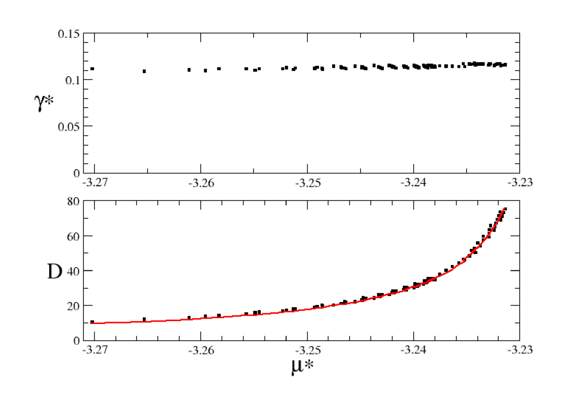
Figure 5: (color on line) Top: Surface tension $\gamma=\frac{L\ell f_{ex}}{\pi D}$ as a function of the chemical potential on the bubble branch. Bottom: Nucleus diameter $D$ versus chemical potential. The points are extracted from the density profiles (with the Gibbs dividing interface) and the red line is the prediction from the classical nucleation theory (see text).

How to use this value for determining nucleation barriers? The crucial point is the shape of the critical nucleus. Tallanquer et al.talanquer (12) showed by local density-functional theory in the gradient approximation that the shape of the critical nucleus can either be attached to one of the walls or can bridge the two walls, depending on the conditions. For a small separation between the walls, the critical nucleus bridges the walls and one can anticipate that nuclei have a round shape in the $(x,y)$ plane. Applying the classical nucleation theory with this hypothesis readily yields the value of the critical diameter $D^{*}$ of the droplet (resp. bubble) as a function of the difference $\Delta\omega$ between the grand-potential densities of the vapor-like (resp. liquid-like) GC metastable state and the liquid-like (resp. vapor-like) GC stable state at a given chemical potential $\mu$ : $D^{*}=\frac{2\gamma}{|\Delta\omega|}$. The corresponding energy barrier is $\Delta\Omega^{*}=\frac{\pi H\gamma^{2}}{|\Delta\omega|}$. These quantities may be rewritten close to the coexistence, where $\rho_{L}(\mu)-\rho_{V}(\mu)\simeq\rho_{L}(\mu_{coex})-\rho_{V}(\mu_{coex})=\Delta\rho$, as $D^{*}=\frac{2\gamma}{\Delta\rho|\mu_{coex}-\mu|}$ and $\Delta\Omega^{*}=\frac{\pi H\gamma^{2}}{\Delta\rho|\mu_{coex}-\mu|}$.

The bubble and droplet branches.

What is the relation between the critical nuclei theoretically described above and the observed bubbles and droplets? As can be seen in Fig. 4 (and expected), the branches associated with the gas-like, liquid-like and rail states are independent of the system size, except for their extension in the $\rho-\mu$ diagram. On the other hand, those associated with the bubble and droplet states exhibit a simple system size dependence as explained now.

Consider for instance a state $(\mu,\bar{\rho})$ on the bubble branch in a box $L\times\ell\times H$. Outside the bubble and its interface, the density is equal to the density of the liquid-like branch $\rho_{L}(\mu)$. If the bubble is sufficiently large, the density inside the bubble is equal to the density of the vapor-like branch $\rho_{V}(\mu)$. Taking advantage of the approximately cylindrical symmetry of the bubble around the $z$-axis, one defines the diameter $D=D(\mu)=2R$ of the bubble as the diameter of the cylindrical surface dividing the two liquid-like and vapor-like phases, which ensures $\bar{\rho}(\mu)=x\rho_{L}(\mu)+(1-x)\rho_{V}(\mu)$ where $x=\frac{V_{L}}{V}$ and $V_{L}$ the volume of the liquid-like phase. The free-energy density $\bar{f}$ of the system can then be written as $\bar{f}=xf_{L}(\mu)+(1-x)f_{V}(\mu)+f_{ex}$. For large bubbles ($D>>1$), we have checked that $x\simeq\frac{\pi D^{2}}{4L\ell}$ and that $\frac{L\ell f_{ex}}{\pi D}$ is almost constant with the chemical potential (see Fig. 5) and equal to the surface tension $\gamma$ previously determined. (We have not found any noticeable influence of the interface curvature.)

Consistent with this approximation is that the distance in chemical potential from the liquid-vapor coexistence is small. The Kelvin equation should then be valid so that $|\mu-\mu_{coex}|=\frac{2\gamma}{\Delta\rho D}$ as illustrated in Fig. 5: this means that the bubble (and droplet) branches are the locus of the critical nuclei introduced above. Finally, one finds the expression of the bubble-branch equation,

$$\bar{\rho}(\mu)=\rho_{L}(\mu)-\frac{\pi}{HL\ell}\frac{H\gamma^{2}}{\Delta\rho|\mu_{coex}-\mu|^{2}}\,,$$ (8)

which makes their size dependence explicit. The curves all collapse when one plots $HL\ell\bar{\rho}(\mu)=N(\mu)$ as a function of $\mu$.

The morphological transitions.

One cannot find analytically the density of the transition between the vapor-like and the droplet branch. Physically, the transition takes place when the adsorbed film can supply enough fluid to form the droplet. Data inspection shows that the smallest possible (stable) droplet is essentially independent of system size, but what about the equilibrium droplet at the transition? We have found that the size of the equilibrium droplet grows with the system size and, accordingly, that the corresponding chemical potential decreases to $\mu_{coex}$.

On the other hand, the transition between the droplet and rail states is essentially controlled by the geometry of the system. The excess free energies of these states are indeed the product of the surface tension $\gamma$ by the perimeter of the interface: $2\ell$ for the rail ($\ell<L$), $\pi D$ for the droplet. Equality of these excess free energies leads to the following values on the droplet branch at the transition: $(\bar{\rho}-\rho_{V})/(\rho_{L}-\rho_{V})=\frac{1}{\pi}\frac{\ell}{L}$ and $\mu=\mu_{coex}+\frac{\pi\gamma}{H\Delta\rho\ell}$. Note that for square systems, $\rho$ at the transition does not depend on the system size, as illustrated in Fig. 4. The same relation applies for the transition between the rail and the bubble states (with the exchange $L\leftrightarrow V$). These transitions can never be avoided: the system, for instance on adsorption, will always visit first the droplet state, then the rail state and finally the bubble state.

III.2 Monte Carlo Results

III.2.1 Adsorption/desorption isotherms

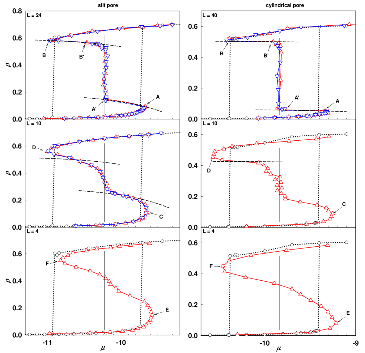
Figure 6: Left panel: Adsorption (up triangles) and desorption (down triangles) isotherms of a Lennard-Jones fluid in a slit pore of height $H=6$, width $\ell=8$, and lengths $L=4,10,$ and $24$ from bottom to top. Right panel: Same as left for a cylindrical pore of diameter $D=6$ and lengths $L=4,10,$ and $40$ from bottom to top. For the smallest lengths the desorption isotherms are indistinguishable from the adsorption and are therefore not shown. The relative size of the reservoir with respect to the pore is 66.7 for the slit pore and 50 for the cylinder; for these values, the conditions are close to canonical for the fluid in the pore. Labels A to F are used in subsequent figures. The open circles and dotted lines denote the grand-canonical adsorption and desorption isotherms obtained for the largest $L$. The dashed lines represent the canonical constraint for the total system comprising the pore and the reservoir for some specific points along the isotherms. The vertical thin lines materialize the coexistence points.

The measured amount of fluid in the pore upon isothermal adsorption or desorption, as obtained in the atomistic model, is shown in Fig. 6. In both pore geometries (slit and cylinder) the pore length drastically influences the results. The pore length $L$ varies between 4, a value slightly smaller than its width or diameter, to significantly larger values ensuring high aspect ratios. The drastic changes occur for the smallest values of $L$. All isotherms then exhibit reversibility and a typical continuous $S$-shape. Increasing $L$ progressively leads to a deformation of the isotherms with the appearance of a steeper portion in the center. For large enough $L$, the isotherms exhibit two discontinuities (associated with morphological transitions) and three separated branches: the lowest-density one corresponds to a monolayer of fluid adsorbed at the walls; the highest-density one corresponds to a dense liquid-like filling the pore. In both cases the density profile describing the fluid is homogeneous in the direction parallel to $L$. On the other hand, the third branch of intermediate density corresponds to an inhomogeneous fluid state, made of fluid menisci or bridges anchored at the walls.

Grand canonical simulations were performed in the largest systems, close to the thermodynamic limit (shown as circles and dotted lines in Fig. 6). As can be seen, the low- and high-density branches closely follow those obtained in the grand-canonical ensemble, except for the smallest system due to finite-size effects. Note also the small differences in the limits of stability, even in the largest systems. The mesoscopic canonical ensemble attenuates fluctuations, thereby stabilizing the metastable branches.

What happens around the discontinuities? The total system comprising the pore and the reservoir is in the canonical ensemble. The corresponding constraint between the chemical potential and the amount of fluid in the pore appears as dashed lines. Note that if the pore were in the canonical ensemble, the constraint would result in horizontal dashed lines. In our case, the ratio between the reservoir size and the pore size (66.7 for the slit pore and 50 for the cylinder) is such that the pore is close to the canonical situation. As can be seen, for the largest systems, after the limit of stability of the low- and high-density branches are reached, the isotherm follows these constraints.

III.2.2 Grand potential calculations

The fluid grand-potential density in the pore $\Pi_{\rm P}$ was calculated during the course of the simulation, by using the direct algorithm when possible [Eq. (5)]. It was also computed by thermodynamic integration of the Gibbs relation $d\Pi=\rho d\mu$ along the adsorption isotherm. For clarity, the results are given as a function of the point label (points are labeled from the beginning of the adsorption in the gas regime to the full filling of the pore by the liquid) in order to avoid superimposition of points (see Fig. 7). Note that the applicability of the thermodynamic integration is not straightforward since the adsorption/desorption isotherms are discontinuous (while reversible). By convention, discontinuities are integrated as single (large) increments. The associated error will be rigorously evaluated in next section.

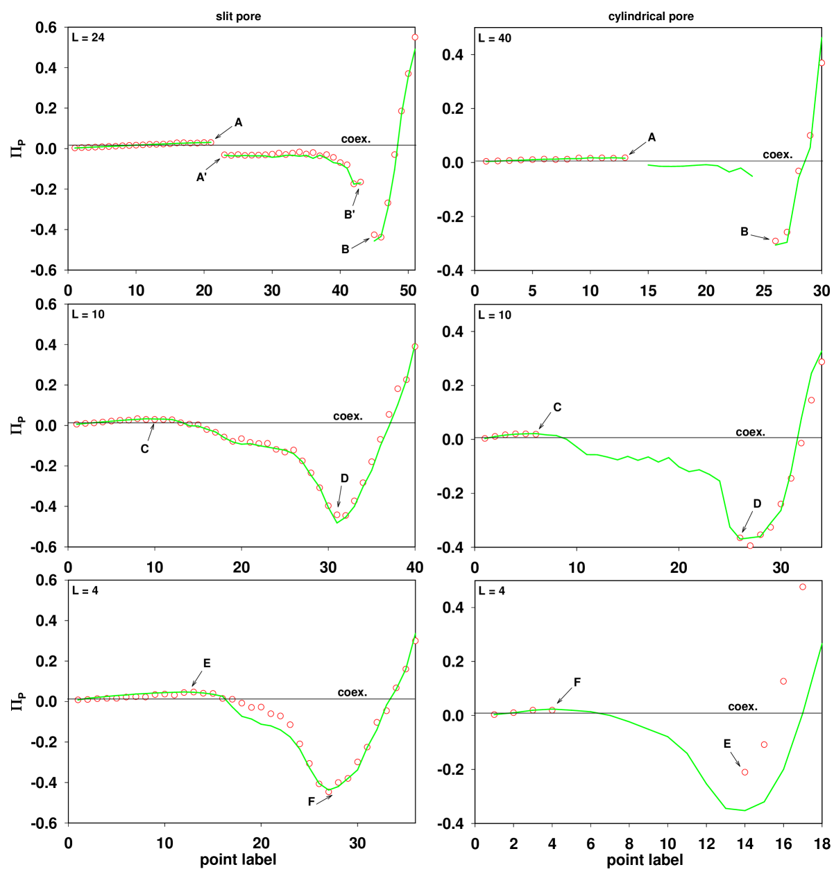
Figure 7: Grand-potential density, $\Pi_{\rm P}=-\Omega_{\rm P}/V_{\rm P}$, of the fluid in the pore along the adsorption isotherm. The data are given as a function of the occurrence number of the points along the isotherm, the points being labeled from the beginning of the adsorption in the gas regime to the full filling of the pore by the liquid. Labels A to F are the same as in Fig 6. Solid lines: thermodynamic integration of the Gibbs relation $d\Pi=\rho d\mu$. Symbols: direct computation using Eq. 5 when possible (density profiles homogeneous in at least one direction, see text). Left panel: slit pore of height $H=6$, width $\ell=8$, and lengths $L=4,10,$ and $24$ from bottom to top. Right panel: cylindrical pore of diameter $D=6$ and lengths $L=4,10,$ and $40$ from bottom to top. The horizontal thin lines materialize the coexistence value of the grand potential density in the thermodynamic limit.

Let us first focus on the gas-like and liquid-like branches of the isotherms, which correspond to fluid configurations that are uniform along the pore axis. The thermodynamic results can be compared to the direct algorithm [Eq. (5)]. A disagreement is observed between the two methods for the smallest cylindrical pore ($L=4$), most probably due to trivial finite size effects. Otherwise, for all other systems, the agreement is excellent, validating the thermodynamic integration of the grand potential along the isotherms. This result is quite remarkable since the isotherms exhibit discontinuities.

For the intermediate region of the isotherms, corresponding to a backward evolution of the chemical potential with the fluid density in the pore, the fluid configurations are inhomogeneous along the direction $L$, with a rail (resp. droplet) of liquid on the low-density side, and a cylinder (resp. bubble) of gas on the high-density side for the slit (resp. cylindrical) pore. As a consequence, the direct method is expected to fail and the corresponding results are not shown. However, the case of the slit pore can be considered more carefully. In this geometry, for a large enough length $L>\ell=8$, visual inspection of the configurations shows that the orientation of the liquid rail or of the gas cylinder is always parallel to the direction $\ell$, ie, the fluid is uniform along this direction. The direct method can thus be applied with the virtual variations performed along $\ell$. (We checked that for the homogeneous gas-like and liquid-like branches the results are identical to those obtained with virtual variations along $L$.) The interesting results are those obtained in the inhomogeneous intermediate region. As seen from Fig. 7, the thermodynamic integration results coincide with those obtained directly during the course of the simulation for $L=10$ and $24$. For the smallest length $L=4$ a disagreement appears. Visual inspection of the atomic configurations shows that the direction of the liquid rail or of the gas cylinder fluctuates between the $\ell$ and $L$ directions: as a consequence, the direct method actually fails, and the results should not be compared to thermodynamic integration.

The global picture that arises is that for large enough systems (to avoid spurious finite-size effects), the thermodynamic integration is a rational route to obtain the grand potential. The analytical calculation of the errors associated with the discontinuities (see next section) validates this observation.

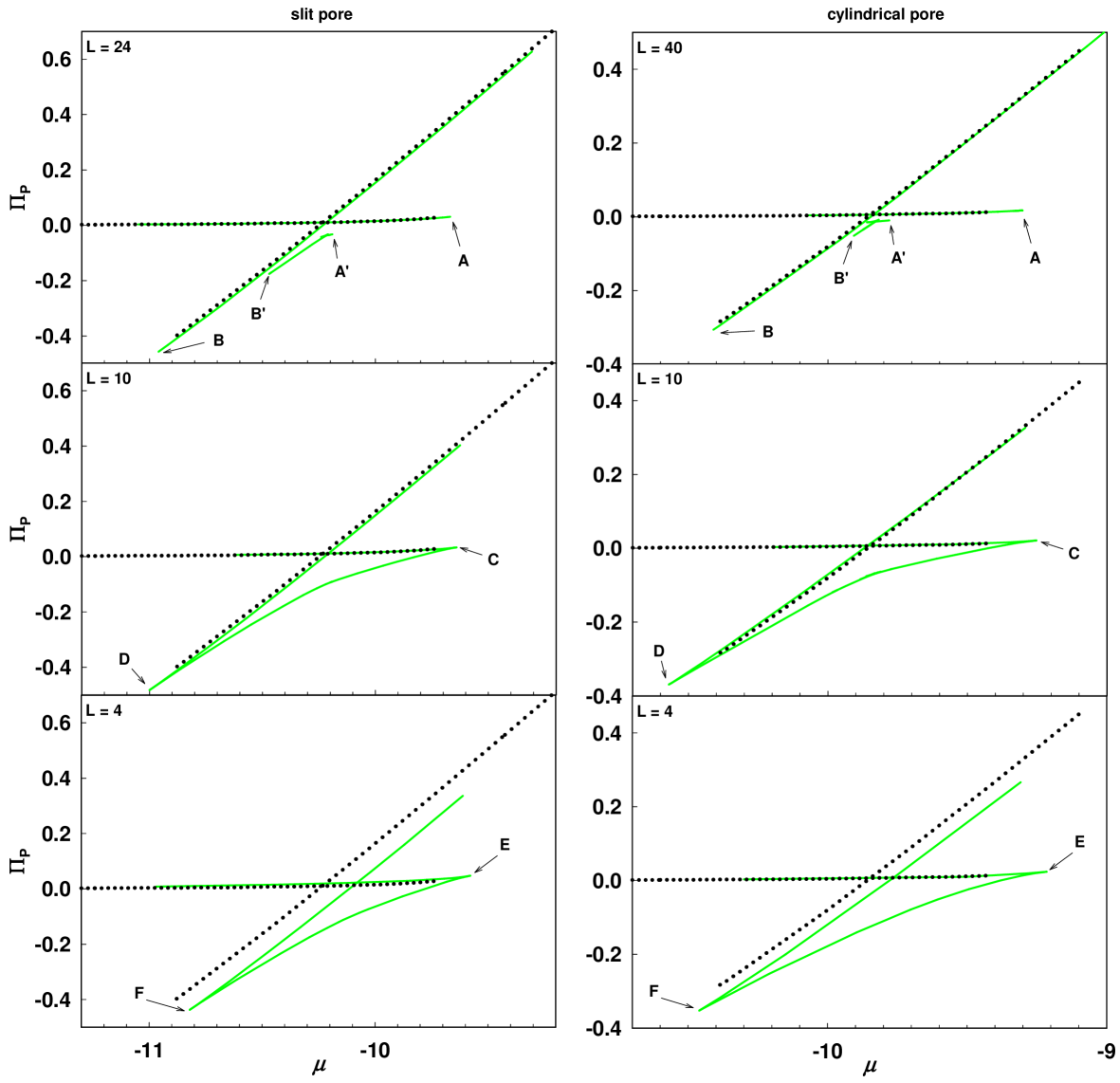
Figure 8: Grand-potential density, $\Pi_{\rm P}=-\Omega_{\rm P}/V_{\rm P}$, of the fluid in the pore versus fluid chemical potential $\mu$. Labels A to F are the same as in Fig 6. Solid lines: thermodynamic integration of the Gibbs relation $d\Pi=\rho d\mu$. Dotted lines: grand-canonical computation performed in a pore long enough for representing the thermodynamic limit. Left panel: slit pore of height $H=6$, width $\ell=8$, and lengths $L=4,10,$ and $24$ from bottom to top. Right panel: cylindrical pore of diameter $D=6$ and lengths $L=4,10,$ and $40$ from bottom to top.

Fig. 8 (solid lines) shows the evolution of the grand-potential density obtained by thermodynamic integration versus the chemical potential $\mu$. There are two principal branches with very different slopes (given by the density of the adsorbed fluid), corresponding to the gas-like and liquid-like portions of the isotherms. These branches cross at coexistence between the gas-like and liquid-like states. For the lowest values of $L$, these branches are connected by a continuous line corresponding to the backward portion of the isotherm. On the other hand, for the largest values of $L$, the line associated with the inhomogeneous intermediate states appear as a separate branch just below the coexistence point. The difference in grand potential between these states and the coexistence point is due to the contributions of the two gas/liquid interfaces of the nonuniform states (the corresponding grand potential is higher). The numerical calculations give a reduced surface tension of 1.25 for both systems and for $L\geq 10$.

The grand-potential density obtained by thermodynamic integration can be compared to a grand-canonical computation performed on the largest pores (that are closer to the thermodynamic limit). The results of the grand-canonical computation are available only for the gas-like and liquid-like branches (see Figs. 6 and 8, dotted lines). Fig. 8 shows that, along these branches, the agreement with the results of thermodynamic integration is excellent for the largest length and for the two geometries. The agreement however deteriorates as one considers smaller lengths for the thermodynamic integration. It is not a failure of the thermodynamic integration, but finite-size effects then affect the calculations. This is clearly visible in the isotherms (see Fig. 6).

III.2.3 Thermodynamic integration

The question we now address follows from the previously observed numerical agreement between the grand-potential calculations and the thermodynamic integration of the adsorption isotherms. Is it valid to calculate the fluid “grand potential” in the pore $\Omega_{\rm P}$ by a direct integration of $\left<N_{\rm P}\right>(\mu)$ along the isotherm when the latter is reversible yet discontinuous? Note that the relation we consider here involves the average number of atoms in the pore, not the total number of atoms in the whole system. Integration is obviously possible along the continuous portions of the adsorption branches. A difficulty arises when discontinuities (gaps) are present, which may then introduce sizeable errors and even invalidate the procedure. By using the fact that the total number of particles $N$ and the total free energy $F$ are the same on both sides (labeled 1 and 2) of a given gap, one has from Eq. 7:

$${\Omega_{P,1}-\Omega_{P,2}} =-(\mu_{2}-\mu_{1})N-\left(\Omega_{R,2}-\Omega_{R,1}\right)$$ (9)

$$=-(\mu_{2}-\mu_{1})\frac{\left<N_{P,2}\right>+\left<N_{P,1}\right>}{2}-\Delta$$

with

$$\Delta=(\mu_{2}-\mu_{1})\frac{\left<N_{R,2}\right>+\left<N_{R,1}\right>}{2}+\left(\Omega_{R,2}-\Omega_{R,1}\right){\rm.}$$ (10)

In these expressions, $P$ and $R$ denote the pore and reservoir contributions.

The term $-(\mu_{2}-\mu_{1})\frac{\left<N_{P,2}\right>+\left<N_{P,1}\right>}{2}$ of Eq. 9 exactly corresponds to what would be obtained by applying the usual thermodynamic integration of $\left<N_{\rm P}\right>(\mu)$ via a discrete integration performed over simulation points, in which the discontinuity $1-2$ is considered as a single increment. $\Delta$ is the difference between the grand potential calculated by thermodynamic integration and the true one. To evaluate this term we use the ideal-gas expressions for $N_{\rm R}(\mu)$ and $\Omega_{\rm R}(\mu)$. An expansion in terms of the chemical potential difference $\mu_{2}-\mu_{1}$ then leads to

$$\Delta=(\mu_{2}-\mu_{1})^{3}\frac{\left<N_{R,1}\right>}{12k_{B}^{2}T^{2}}+O((\mu_{2}-\mu_{1})^{5})\,,$$ (11)

or alternatively in terms of the difference in adsorbed amount $\left<N_{P,2}\right>-\left<N_{P,1}\right>=\left<N_{R,1}\right>-\left<N_{R,2}\right>$, to

$$\Delta=(\left<N_{P,1}\right>-\left<N_{P,2}\right>)^{3}\frac{k_{B}T}{12\left<N_{R,1}\right>^{2}}$$

$$+O((\left<N_{P,1}\right>-\left<N_{P,2}\right>)^{5}){\rm.}$$ (12)

Note that either in the canonical ensemble ($\left<N_{P,1}\right>=\left<N_{P,2}\right>$) or in the grand-canonical ensemble ($\mu_{1}=\mu_{2}$), the integration is exact ($\Delta=0$ to all orders). In a generic mixed (or mesoscopic-canonical) ensemble, the integration is not exact, but the above equations show that the standard thermodynamic integration of $\left<N_{\rm P}\right>(\mu)$ gives the grand potential within an error of order 3 in the gap $1-2$. If the observed gaps are small, and in particular not much larger than the increments between two simulation points, the error introduced is negligible compared to the second order error introduced by the discrete integration procedure.

The last point to be discussed is what happens if the fluid in the reservoir is not ideal, as for instance close to the critical point? In this case, the last term $\left(\Omega_{R,2}-\Omega_{R,1}\right)$ in Eq. (9) should be replaced by $\int_{1}^{2}d\mu\left<N_{\rm R}\right>(\mu)$, which corresponds to a thermodynamic integration of the fluid properties from state 1 to state 2 in the whole system. This shows that the error introduced by the thermodynamic integration of $\left<N_{\rm P}\right>(\mu)$ is the difference between the continuous and the discrete integral of $\left<N_{\rm R}\right>(\mu)$ between points 1 and 2 and therefore is now of order 2 in the gap $1-2$. (Note that if this gap is of the order of the increment between simulation points, the error is of the same order of magnitude as the one due to the discrete integration.)

We can summarize the above discussion as follows: If the isotherm obtained in the mixed (mesoscopic-canonical) ensemble is reversible and exhibits small gaps, thermodynamic integration can be safely performed to calculate the grand potential of the confined fluid. The size of the pore must be large enough for ensuring that the result of thermodynamic integration in a finite-size system coincides with the thermodynamic limit. If the gaps are large but the fluid is ideal in the reservoir (far from the critical point for instance), the error is expected to be of order 3 in $\mu_{2}-\mu_{1}$ or $\left<N_{P,1}\right>-\left<N_{P,2}\right>$, and thus quite small. If the fluid is not ideal in the reservoir, the error is of second order. In the latter case, determining the total Helmholtz free energy $F$ by thermodynamic integration and using Eq. (7) is then a better route.

IV Conclusion

In this paper we have studied the influence of the system size on the properties of a fluid adsorbed in a nanopore, when the reservoir is small enough to enforce canonical or near-canonical ensemble conditions for the adsorbed fluid. The system here refers to the pore, which is chosen of simple, slit or cylinder, geometry. We have done so by means of two complementary methods: the density-functional theory for a lattice-gas model and Monte Carlo simulations of an atomistic model. The motivation behind the study was two-fold: first, a theoretical investigation of the inhomogeneous fluid states that can be stabilized in the canonical ensemble for a finite-size system and, second, an assessment of the “gauge-cell method”neimark (02) that was devised for computing thermodynamic quantities in numerical studies.

Within the density-functional approach, we have obtained results that can be summarized as follows:

• The path followed by the system on adsorption and desorption depends crucially on the system size and on the degrees of freedom allowed for the density profiles.

• Large systems exhibit morphological transitions between “homogeneous” phases (more precisely, phases having the symmetry imposed by the geometry of the pore) and inhomogeneous phases (where the symmetry is broken). Hysteresis can moreover be suppressed and equilibrium found since the density-functional theory provides the free-energy values.

• Among the branches of the isotherms associated with inhomogeneous fluid phases, the droplet and bubble branches are found as the loci of the critical nuclei with properties that are consistent with the classical nucleation theory.

• Continuous and reversible isotherms are observed in small systems. However, when increasing system size, the symmetries of the external potential imposed by the pore can be broken for the density profiles and we have devised a technical trick to obtain such profiles in a density-functional theory.

On the other hand, via the Monte Carlo simulations:

• We have focused on the idea, which is behind the gauge-cell method, of using small systems to get a continuous van der Waals-like isotherm from which thermodynamic integration could be safely implemented. We have found that when going to the small system sizes required to observe continuous isotherms, the thermodynamic properties are strongly affected by the limited size, especially in computer simulations where the required system size becomes smaller than the range of the interactions. Indeed, inhomogeneous states persist down to quite small system sizes so that the recovery of an $S$-shape quasi-continuous isotherm is very slow when decreasing the size. This procedure is therefore not a good way to extract the thermodynamic properties of the adsorbed fluid.

• We have suggested an alternative method, in which the system (pore) size is reduced only until a reversible isotherm is found, even if discontinuities are present. The size is larger than in the above case and the properties of the gas-like and liquid-like branches of the isotherms are not altered with respect to the thermodynamic limit. We have shown that thermodynamic integration is still valid in the presence of jumps, provided that the isotherm is reversible. This is an extension of the gauge-cell method to cases where inhomogeneous states and morphological transitions are present.

We finally note that our study supports the view that playing with system and reservoir size (as well as with temporary modifications of the external potential exerted by the pore on the fluid) seems to be a very generic route to numerically investigate nucleation and the associated free-energy barriers in adsorbed fluids.

References

- neimark (02) A. V. Neimark, P. I. Ravikovitch, and A. Vishnyakov, Phys. Rev. E 65, 031505 (2002).
- puibasset (09) J. Puibasset, E. Kierlik, and G. Tarjus, J. Chem. Phys. 131, 124123 (2009).
- kierlik (09) E. Kierlik, J. Puibasset, and G. Tarjus, J. Phys.: Condens. Matter 21, 155102 (2009).
- pana (87) A. Z. Panagiotopoulos, Mol. Phys. 61, 813 (1987).
- smit (89) B. Smit, P. De Smedt, and D. Frenkel, Mol. Phys. 68, 931 (1989).
- smit (89b) B. Smit and D. Frenkel, Mol. Phys. 68, 951 (1989).
- neimark (00) A. V. Neimark and A. Vishnyakov, Phys. Rev. E 62, 4611 (2000).
- neimark (05) A. V. Neimark and A. Vishnyakov, J. Phys. Chem. B 109, 5962 (2005).
- neimark (05b) A. V. Neimark and A. Vishnyakov, J. Chem. Phys. 122, 054707 (2005).
- neimark (05c) A. V. Neimark and A. Vishnyakov, J. Chem. Phys. 122, 234108 (2005).
- vishny (03) A. Vishnyakov and A. V. Neimark, J. Chem. Phys. 119, 9755 (2003).
- kierlik (02) E. Kierlik, P. A. Monson, M.L. Rosinberg, and G. Tarjus, J. Phys.: Condens. Matter. 14, 9295 (2002).
- detcheverry (03) F. Detcheverry, E. Kierlik, M.L. Rosinberg, and G. Tarjus, Phys. Rev. E 68, 061504 (2003).
- Maier (01) R. W. Maier and M. A. Stadtherr, AIChE Journal 847, 1874 (2001).
- puibasset (05) J. Puibasset, J. Phys. Chem. B 109, 4700 (2005).
- puibasset (05b) J. Puibasset, J. Chem. Phys. 122, 134710 (2005).
- eppenga (84) R. Eppenga and D. Frenkel, Mol. Phys. 52, 1303 (1984).
- harismiadis (96) V. I. Harismiadis, J. Vorholz, and A. Z. Panagiotopoulos, J. Chem. Phys. 105, 8469 (1996).
- vortler (00) H. L. Vörtler and W. R. Smith, J. Chem. Phys. 112, 5168 (2000).
- monson (08) P. A. Monson, J. Chem. Phys. 128, 084701 (2008).
- everett (72) D. H. Everett and J. M. Hayes, J. Colloid and Interface Sci. 38, 125 (1972).
- schrader (09) M. Schrader, P. Virnau and K. Binder, Phys. Rev. E 79, 061104 (2009).
- binder (03) K. Binder, Physica A 319, 99 (2003).
- binder (12) K. Binder, B. J. Block, P. Virnau and A. Tröster, Am. J. Phys. 80, 1099 (2012).
- talanquer (12) V. Talanquer and D. W. Oxtoby, J. Chem. Phys. 100, 5190 (1994).