Intrinsic physical properties and Doppler boosting effects in LS I +61^∘303

Abstract

Aims. Our aim is to show how variable Doppler boosting of an intrinsically variable jet can explain the long-term modulation of $1667\pm 8$ days observed in the radio emission of LS I +61^∘303.

Methods. The physical scenario is that of a conical, magnetized plasma jet having a periodical ($P_{1}$) increase of relativistic particles, $N_{\rm rel}$, at a specific orbital phase, as predicted by accretion in the eccentric orbit of LS I +61^∘303. Jet precession ($P_{2}$) changes the angle, $\eta$, between jet axis and line of sight, thereby inducing variable Doppler boosting. The problem is defined in spherical geometry, and the optical depth through the precessing jet is calculated by taking into account that the plasma is stratified along the jet axis. The synchrotron emission of such a jet was calculated and we fitted the resulting flux density $S_{\rm model}(t)$ to the observed flux density obtained during a 6.5-year monitoring of LS I +61^∘303 by the Green Bank radio interferometer.

Results. Our physical model for the system LS I +61^∘303 is not only able to reproduce the long-term modulation in the radio emission, but it also reproduces all the other observed characteristics of the radio source, the orbital modulation of the outbursts, their orbital phase shift, and their spectral index properties. Moreover, a correspondence seems to exist between variations in the ejection angle induced by precession and the rapid rotation in position angle observed in VLBA images.

Conclusions. The peak of the long-term modulation occurs when the jet electron density is around its maximum and the approaching jet is forming the smallest possible angle with the line of sight. This coincidence of maximum number of emitting particles and maximum Doppler boosting of their emission occurs every $\sim$1667 days and creates the long-term modulation observed in LS I +61^∘303.

1 Introduction

A recent timing analysis of the GBI radio data of LS I +61^∘303 has revealed two frequencies: $P_{1}={1\over\nu_{1}}=26.49\pm 0.07\,\mathrm{days}$ and $P_{2}={1\over\nu_{2}}=26.92\pm 0.07\,\mathrm{days}$ (Massi & Jaron 2013). The period $P_{1}$ agrees with the value of $26.4960\pm 0.0028\,\mathrm{days}$ (Gregory 2002) associated to the orbital period of the binary system formed by a compact object and a Be star (Grundstrom et al. 2007). Period $P_{2}$ agrees with the previous estimate of 27-28 days by radio astrometry of the precessional period of the radio structure (Massi et al. 2012).

The timing analysis results seem to confirm LS I +61^∘303 as the second case of a radio-emitting X-ray binary with precessional period ($P_{2}$) of its radio jet very close to the orbital ($P_{1}$) period of the binary system (Massi et al. 2012; Massi & Jaron 2013). Whereas the several known precessing X-ray binaries (Larwood 1998) have a precession period an order of magnitude longer than the orbital period (as predicted for a tidally forced precession by the companion star), the different case of GRO J1655-40 was discovered in 1995 (Hjellming & Rupen 1995). This black hole candidate, which has an orbital period of 2.601$\pm 0.027$ days (Bailyn et al. 1995), revealed a radio jet with a precessional period of 3.0$\pm$0.2 days (Hjellming & Rupen 1995). LS I +61^∘303 is a high-mass X-ray binary, and GRO J1655-40 is a low-mass X-ray binary. The mechanism proposed in both cases to explain the precession is based on general relativity effects around the compact object. Lense-Thirring precession has been analysed for GRO J1655-40 by Martin et al. (2008) and for LS I +61^∘303  by Massi & Zimmermann (2010).

When two frequencies are only slightly different, a beating results, i.e. an interference producing a new frequency: their average, $\nu_{\rm average}={{\nu_{1}+\nu_{2}}\over 2}$, which gets modulated with the beat frequency, $\nu_{\rm beat}=\nu_{1}-\nu_{2}$. As shown in Massi & Jaron (2013) for LS I +61^∘303 , the term $1/\nu_{\rm beat}$ results $1667\pm 393\,\mathrm{days}$ and is compatible with the observed long-term modulation of the radio flux density of $1667\pm 8$ days, attributed in the past to variations in the wind of the Be star (Gregory & Neish 2002). Evidence of beating in LS I +61^∘303 comes from the fact that the periodicity of the radio outbursts is indeed the one predicted by the beat theory, which is $P_{\rm outburst}=P_{\rm average}={1\over\nu_{\rm average}}=26.70\pm 0.05$ days (Massi & Jaron 2013; Jaron & Massi 2013). Since the the two frequencies $\nu_{\rm average}$ and $\nu_{\rm beat}$ are related , the long-term modulation should also be a result of the beating process between $P_{1}$ an $P_{2}$.

The aim of this paper is to prove, in the context of a physical scenario, how the mutual relationship between $P_{1}$ and $P_{2}$ can generate the long-term periodicity. We linked the two periodicities, $P_{1}$ and $P_{2}$, to two physical processes: the periodical ($P_{1}$) increase of relativistic electrons in a conical jet and the periodical ($P_{2}$) Doppler boosting of the emitted radiation by relativistic electrons because of jet precession. The hypothesis that the compact object in LS I +61^∘303, accreting material from the Be wind, undergoes a periodical ($P_{1}$) increase in the accretion at a particular orbital phase along an eccentric orbit was suggested and developed by several authors (Taylor et al. 1992; Marti & Paredes 1995; Bosch-Ramon et al. 2006; Romero et al. 2007). The hypothesis that a precessing jet, with an approaching jet having large excursions in its position angle, should give rise to appreciable Doppler boosting effects is supported by the morphology of Massi et al. (2004), Dhawan et al. (2006), and Massi et al. (2012) images showing extended radio structures changing from two-sided to one-sided morphologies at different position angles.

Our model describes a precessing ($P_{2}$) jet with a periodically ($P_{1}$) varying number of relativistic electrons. Section 2 describes our analytical model and how to calculate its flux density $S_{\rm model}$. In Sect. 3, all parameters for calculating $S_{\rm model}$ are derived by fitting the model to 6.5 years of GBI radio flux density observations. In Sect. 4 we present our results and in Sect. 5 our conclusions.

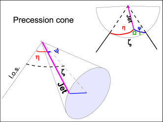
Figure 1: Precessing jet and relative angles. Left: Sketch of the precessing cone. The angle $\zeta$ is the angle between the jet precession axis and the line of sight (l.o.s.) direction, $\psi$ is the opening angle of the precession cone and $\eta$ is the continuosly changing angle between the jet and the line of sight because of precession. Right: The angles $\zeta$,$\eta$,$\psi$ in spherical geometry. The angle $\Omega$, describing in the precession period $P_{2}$ an angle $2\pi$, defines the temporal dependence.

2 Model definition

In this section we want to analytically determine the flux density of a precessing radio jet having a periodical variation in the number of its emitting particles. Section 2.1 describes the type of emitting source we are assuming for our model, which is the conical jet used for microquasars and AGNs after the seminal paper of Blandford & Königl (1979). In particular, we adopt Kaiser’s analytical treatment (Kaiser 2006) to express the changes of magnetic field and plasma properties along the jet axis. The flux density of our jet, which is $S_{\rm model}$ in Eq. 1, contains two contributions: the Doppler factors and the intrinsic synchrotron emission of the conical jet. The Doppler factors are determined in Sect. 2.2.

The most important parameter introduced to define the Doppler boosting term is the angle $\eta$ between jet axis and line of sight. This is the angle that continuously varies because of precession. Section 2.3 deals with the second contribution of Eq. 1, i.e., the intrinsic synchrotron emission of the conical jet. The difference with respect to Kaiser’s model, where the jet is seen at $\eta\sim 90^{o}$, is that here we are dealing with a precessing jet, i.e., with a continuously varying angle $\eta$. This implies the calculation of the optical depth through a stratified jet (Sect. 2.3 and Appendix). Also, in our case, the number of relativistic particles, $N_{\rm rel}$, changes along the orbit of LS I +61^∘303, as described in Sect. 2.4.

2.1 The model

The general framework for LS I +61^∘303 emission in the radio energy range is that of synchrotron radiation emitted from a relativistic electron population of density $N_{\rm rel}$ moving in a magnetic field $B$. However, this simple scenario does not reproduce the radio spectra of LS I +61^∘303. A simple magnetized plasma containing particles with a power-law energy distribution produces a power-law spectrum ($S\propto\nu^{\alpha}$) with spectral slope $\alpha<0$ above the critical frequency, while below this critical frequency self-absorption effects become important and the emission becomes optically thick with a spectral slope $\alpha$=2.5 (Longair 1994; Kaiser 2006). This spectrum of a uniform, self-absorbed synchrotron source is not the kind of radio spectrum observed in LS I +61^∘303. The optically thick emission observed in LS I +61^∘303 is much flatter with $\alpha$ in the range of $0.0-0.5$ (Massi & Kaufman Bernadó 2009; Zimmermann 2013), similar to the values $\alpha\sim 0.0-0.6$ observed in microquasars (Fender 2001). Optically thick synchrotron emission in microquasars and in radio loud AGN is modelled with conical jets where changes in magnetic field and plasma density along the flow give rise to the observed flat spectra (Blandford & Königl 1979; Kaiser 2006).

In the framework of this kind of jet model, described by unconstant physical quantities, we follow Kaiser’s model for adiabatic jets (Kaiser 2006), to which one can refer for more details. We use his notation when not otherwise specified. We therefore assume a conical jet, where all quantities are radially constant and change only along the jet axis $x$, with $x$ expressed as $x=x_{0}l$, where $x_{0}$ is an arbitrary position along the $x$-axis defining the dimensionless coordinate $l$ (see Fig. A1 in Appendix). The cone radius is $r(l)=r_{0}l^{a_{1}}$, and we choose $a_{1}=1$ to have a cone with a constant opening angle $\xi$ (in Kaiser’s notation $\tan\xi=r_{0}/x_{0}$).

The evolution of the strength of the magnetic field along the jet is parametrized as in Kaiser (2006) as $B=B_{0}l^{-a_{2}}$. Depending on the magnetic field geometry, a purely parallel magnetic field $B\equiv B_{\parallel}$ to the jet axis or a purely perpendicular magnetic field $B\equiv B_{\perp}$ to the jet axis imply different values for $a_{2}$. From Kaiser’s Table 1 we have for $B\sim B_{\parallel}$, $a_{2}=2$, while for $B\sim B_{\perp}$, $a_{2}=1$. As a matter of fact, the most likely configuration is a helical magnetic field configuration with both the parallel and the perpendicular components. Therefore, in the procedure described in Sect. 3 we have calculated the jet emission in both of these limiting cases.

The number density of the relativistic electrons has the usual power-law dependency on the electron energy: $N_{\rm rel}=\kappa E^{-p}$. As in Kaiser (2006), we represent the evolution of the electron distribution density along the jet by setting $\kappa=\kappa_{0}l^{-a_{3}}$, with $a_{3}=2(2+p)/3$ and $p=1.8$ (see Sect. 4.1). But in our case we also introduce a temporal dependence for electron density, setting $\kappa_{0}$ as function of time with periodicity $P_{1}$ (see Sect. 2.4).

In this framework we express the total flux density of the two jets, the approaching, and the receding jet, as

$$S_{\rm model}(t)=S_{\rm a}(t)(\delta_{\rm a}(t))^{k-\alpha}+S_{\rm r}(t)(\delta_{\rm r}(t))^{k-\alpha}$$ (1)

where $\delta_{\rm i}$ is the Doppler boosting term, with i=a for the approaching jet and i=r, for the receding jet. The emission term, $S_{\rm i}(t)$, similarly represents the emission of each jet. Parameter $k$ accounts for the ejecta properties, with $k$=2 for a continuous jet (used here) and $k=3$ for discrete condensations; $\alpha$ is the spectral index.

The quantities $S_{\rm i}$ and $\delta_{\rm i}$ depend on the two physical periodicities $P_{1}$, the orbital period, and $P_{2}$, the precessional period, as described in the following.

2.2 The Doppler boosting effect and its dependency on $P_{2}$

Synchrotron radiation from relativistic electrons spiralling in the magnetic field of the approaching jet becomes enhanced by the Doppler effect (i.e., ”boosted”), while the radiation from electrons of the receding jet becomes attenuated (i.e., ”de-boosted”). Doppler boosting and de-boosting strongly depend on the angle between the jet and the observer’s line of sight (Urry & Padovani 1995; Mirabel & Rodríguez 1999). A precession of the jet implies a variation in this angle and therefore a variable Doppler boosting.

The Doppler boosting and de-boosting terms $\delta_{\rm i}(t)$ are defined as

$$\delta_{\rm a}={\sqrt{1-\beta^{2}}\over 1-\beta\leavevmode\nobreak\ \cos\eta}$$ (2)

$$\delta_{\rm r}={\sqrt{1-\beta^{2}}\over 1+\beta\leavevmode\nobreak\ \cos\eta}$$ (3)

where $\beta={\rm v}/c$ (with ${\rm v}$ the electron velocity component along the jet axis).

Angle $\eta$ is the angle between observer’s line of sight and the jet axis. To follow its changes with time due to the jet precession we express $\eta$ in terms of other quantities, throughout the spherical triangle of sides $\zeta,\psi,$ and $\eta$ shown in Fig.1. Angle $\zeta$ is the angle the jet precession axis makes with the direction of the line of sight. If the jet precession axis is tilted by an angle $f$ with respect to the orbital axis of the binary system, then $\zeta=i+f$, where $i$ is the system inclination angle; $\psi$ is the opening angle of the cone described by the jet during its precession period, $P_{2}$. In the spherical triangle of Fig. 1, the angle $\Omega,$ between sides $\psi$ and $\zeta$, changes with time because of precession and is defined as

$$\Omega=2\pi(t-t_{0}+\Delta)/P_{2},$$ (4)

where $t_{0}$=JD2443366.775 (Gregory 2002, and references therein), and $\Delta$ is the offset to be determined in our model to synchronize $P_{2}$ to $P_{1}$.

From spherical geometry (Smart & Green 1977, Eq. 8) it follows that the time (i.e. $\Omega$) dependency of the angle $\eta$ is

$$\cos\leavevmode\nobreak\ \eta=\cos\leavevmode\nobreak\ \zeta\cos\leavevmode\nobreak\ \psi+\sin\leavevmode\nobreak\ \zeta\sin\leavevmode\nobreak\ \psi\cos\leavevmode\nobreak\ \Omega.$$ (5)

Inserting the $\eta$ expression into Eqs. (2) and (3), we get a temporal modulation of the Doppler boosting factor and we introduce in the observed flux density the dependency on the precession period $P_{2}$.

2.3 Intrinsic jet emission

In our precessing conical jet model, angle $\eta$, between the jet axis and the line of sight, must be clearly variable and can assume all values in the range $90^{o}>\eta>\xi$, with $\xi$ the jet opening angle. This is an important difference with respect to Kaiser’s model, where the jet is seen almost perpendicular to its axis (i.e. $\eta\sim 90^{o}$), or to Potter & Cotter (2012)’s model where the jet is observed at an angle smaller than the opening angle of the jet (i.e., $\eta\leq\xi$).

Since in our model we allow time-dependent values for angle $\eta$, the plasma optical depth also will depend on time. In fact, the optical depth must be computed across the jet along a path that makes an angle $\eta$ with the jet axis and intersects regions characterized by different values of physical quantities (since in our model all quantities vary along the jet axis, i.e., along $x=x_{0}l$) (Fig. A1-Bottom). To make the computation easier, we assume a pyramidal shape for the jet with a square basis of side $2r_{0}l$ and with a lateral surface facing the line of sight. In that way the integration path inside the jet does not depend on other parameters related to the curved jet surface. The perpendicular direction to this surface makes an angle $[90^{o}-(\eta-\xi)]$ with the line of sight for the case of the approaching jet and $[90^{o}-(\eta+\xi)]$ for the receding jet (see Fig. A1-top in the Appendix).

With these assumptions the approaching jet emission can be written as

$$S_{\rm a}=\int^{L}_{1}r_{0}x_{0}I_{\nu_{\rm a}}(\eta,l){\sin(\eta-\xi)\over D^{2}}l{\rm d}l$$ (6)

where $D$ is the distance of LS I +61^∘303 , and the integral is from $l=1$ to $l=L$, with $x_{0}L$ being the jet length and $L$ operationally determined as the limiting value above which there are no more contributions to the jet flux. For the receding jet, we have the same expression with a change of sign in the angular factor that takes the projection of the emitting surface in the direction perpendicular to the line of sight into account. Clearly the difference between the emission of the approaching and of the receding jet becomes negligible for cases where $\xi<<\eta$.

The intensity $I_{\nu}$, emerging from the jet surface, i.e., at $\tau=0$, in the direction $\eta$, is deduced from the radiative transport equation when considering that the plasma inside the jet is stratified along the jet axis direction, i.e., along a direction that makes an angle $\eta$ with respect to the line of sight

$$I_{\nu}(\eta,l)=\int_{0}^{\tau_{\rm end}(l)}{J_{\nu}\over\chi_{\nu}}e^{-\tau^{\prime}/\cos\leavevmode\nobreak\ \eta}\leavevmode\nobreak\ {\rm d}\large\left[{\tau^{\prime}\over\cos\leavevmode\nobreak\ \eta}\large\right],$$ (7)

where $\tau$ is the optical depth defined as

$$\tau(l)=-\int^{\infty}_{l}\chi_{\nu}\leavevmode\nobreak\ {\rm d}x=\tau_{0}l^{1-a_{3}-(p+2)a_{2}/2}.$$ (8)

The upper integration limit $\tau_{\rm end}(l)$ represents the jet optical depth at the specific value of $l$ and takes into account that, at each distance, $x_{0}l$, from the beginning of the jet, the integration path inside the jet involves different regions of the jet itself (see Appendix). The optical depth inside the jet is also a function of the angle $\eta$ (see expressions (A.5) and (A.6)) inducing higher values of the optical depth when the jet is pointing toward the observer, i.e. for low $\eta$ values (but in the limit $\eta\geq\xi$). The consequences of this dependence will be analysed further in a subsequent paper.

The exponent for $l$ in expression (8), when taking Kaiser’s Table 1 into account for all possible $a_{i}$ values, is always negative, so the optical depth is at its maximum at the beginning of the jet:

$$\tau_{0}=\tau(l=1)={\chi_{0}x_{0}\over-[1-a_{3}-(p+2)a_{2}/2]}\nu^{-(p+4)/2}.$$ (9)

Emission and absorption quantities in the above expressions are given, as in Longair (1994) and following the Kaiser (2006) parametrization, by

$$J_{\nu}=J_{0}\nu^{-(p-1)/2}l^{-a_{3}-(p+1)a_{2}/2}\,\mathrm{\leavevmode\nobreak\ }\leavevmode\nobreak\ \leavevmode\nobreak\ \leavevmode\nobreak\ {{W\over{\rm m}^{3}{\rm Hz}}}$$ (10)

$$\chi_{\nu}=\chi_{0}\nu^{-(p+4)/2}l^{-a_{3}-(p+2)a_{2}/2}\,\mathrm{\leavevmode\nobreak\ }\leavevmode\nobreak\ \leavevmode\nobreak\ \leavevmode\nobreak\ {{\rm m^{-1}}},$$ (11)

where

$$J_{0}=2.3\leavevmode\nobreak\ 10^{-25}(1.3\leavevmode\nobreak\ 10^{37})^{(p-1)/2}a(p)B_{0}^{(p+1)/2}\kappa_{0}$$ (12)

and

$$\chi_{0}=3.4\leavevmode\nobreak\ 10^{-9}(3.5\leavevmode\nobreak\ 10^{18})^{p}b(p)B_{0}^{(p+2)/2}\kappa_{0}.$$ (13)

with the constants $a(p)$ and $b(p)$ as in Longair (1994) and $\kappa_{0}$ as determined in the next section.

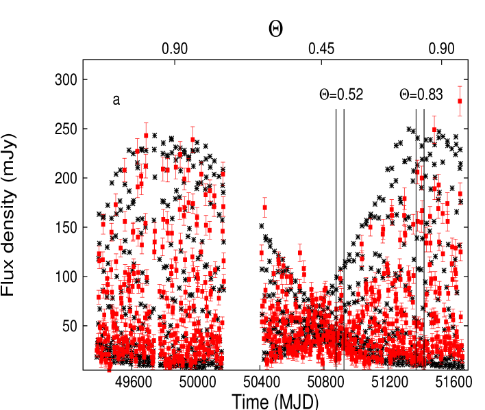
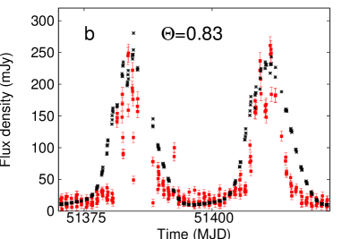
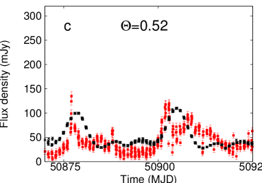
Figure 2: Long-term modulation in LS I +61^∘303. 8.3 GHz GBI observations (red/squares) and model (black/stars) data. a): Model and data vs time (bottom x-axis) and vs the long-term modulation phase $\Theta$ (top x-axis). The long-term modulation phase $\Theta$ is the fractional part of $(t-t_{0})/1667$ with $t_{0}$=JD2443366.775 (Gregory 2002). The GBI data are averaged over 2 days. The four bars define the two time intervals zoomed in Figs. 2 b and 2 c. b) and c): Zoom of two intervals of Fig. 2 a. This (Fig. 2) and all other figures (3, 4, 5, 6, and 7) have been obtained for $B\equiv B_{\parallel}$, $\zeta=46$, $\psi=40$, $\Delta=-922.5$, $\beta=0.28$, $A=3.84$, $\Phi_{r}=0.6$, $L=14$, and $\xi=1.5$ (Sect. 3).

2.4 Periodical increase in relativistic particles along the orbit

To take into account the observed orbital modulation in the radio flux we make the working hypothesis that the relativistic electron input in the jet changes with time. This hypothesis is plausible since as discussed below, the accretion is variable along an eccentric orbit. Our type of representation therefore includes the classical hypothesis that the presence of relativistic electrons in the jet is related to matter accretion on the compact object but makes no hypothesis for how they have been accelerated.

For LS I +61^∘303, with $e=0.72\pm 0.15$ (Casares et al. 2005), the Bondi & Hoyle (1944) accretion theory in an eccentric orbit predicts two maxima (Taylor et al. 1992; Marti & Paredes 1995; Bosch-Ramon et al. 2006; Romero et al. 2007). One maximum is around periastron at $\Phi_{\rm periastron}=0.23\pm 0.02$ (Casares et al. 2005), with the orbital phase $\Phi$ defined as the fractional part of ${(t-t_{0})\over P_{1}}$. However, near periastron the ejected relativistic electrons suffer severe inverse Compton losses because of the proximity to the Be star; a high energy outburst is expected but no or negligible radio emission (Bosch-Ramon et al. 2006). For the second accretion peak, the compact object star is much farther from the Be star, and inverse Compton losses are lower. The relativistic electrons can propagate out of the orbital plane, and we observe a radio outburst (Bosch-Ramon et al. 2006).

In modelling the radio emission we assume a periodical function for relativistic electron density:

$$\kappa_{0}=A\leavevmode\nobreak\ {\it f}(\Phi-\Phi_{\rm r})$$ (14)

where ${\it f}(\Phi-\Phi_{\rm r})$ is equal to 1 for $\Phi=\Phi_{\rm r}$ and expresses (times $A$) the periodical ($P_{1}$) increase in relativistic electrons due to Bondi’s accretion in an eccentric orbit. In this first stage (focussed on Doppler boosting effects and on data periodicity reproduction), we do not include relativistic electron energetic losses but instead allow a different slope for the onset and for the decay so as to take into account that electrons take some time to lose their energy. The top of Fig. 4 shows the resulting $\kappa_{0}$ function for the fit solution illustrated in Figs. 2-7.

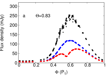
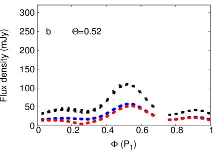
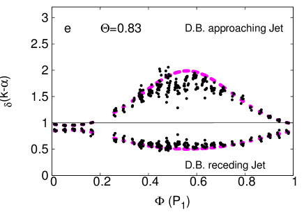
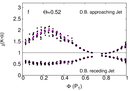
Figure 3: Doppler boosting and intrinsic emission. a-b) $S_{\rm model}$ (black stars), $S_{a}$ (blue line) and $S_{r}$ (red line) of Eq. 1 vs orbital phase $\Phi$, for long-term modulation phases $\Theta=0.83$ and $\Theta=0.52$. c-d) The angle $\eta$ between the jet axis and the line of sight vs orbital phase $\Phi$. e-f) Doppler boosting factors computed with observed spectral index values $\alpha$. The violet curves correspond to Doppler boosting factors computed for $\alpha=-0.4$ (see Sec.4.1).

3 Model fitting

Table 1 reports the parameters, described in the previous section, needed to calculate, by Eq. (1), the flux density of our model, $S_{\rm model}$. The values for the parameters were found by minimizing the $\chi^{2}$ between $S_{\rm model}$, computed at a given $t_{i}$, and the simultaneous observed flux density with the Green Bank interferometer at 8 GHz. That is, we found those values of the parameters that give the lowest value of $\chi^{2}$:

$$\chi^{2}=\sum_{i}{(S_{\rm GBI}(t_{i})-S_{\rm model}(t_{i},parameters))^{2}\over\sigma_{i}^{2}}$$ (15)

where $\sigma$ is the error of GBI data at 8 GHz.

We used the function minimization software MINUIT of the CERN Program Library. In particular, we first set an initial model using the program SCAN, then we optimize the model with the program SIMPLEX to perform the minimization using the simplex method of Nelder & Mead (1965). The best solution is for $B\equiv B_{\parallel}$, $\zeta=46$, $\psi=40$, $\Delta=-922.5$, $\beta=0.28$, $A=3.84$, $\Phi_{r}=0.6$, $L=14$, and $\xi=1.5$. All figures (Figs. 2, 3, 4, 5, 6, and 7) have then been made with this model. However, the non-linearity of the problem makes the solution depending on the initial model, and we also found other solutions with only slight worse fits. This uncertainty is considered in the parameter errors (shown in Table 1) that give the dispersion with respect to the mean value found for each parameter in the different solutions. The solutions for the different magnetic configurations, i.e. cases with $B\equiv B_{\parallel}$ or $B\equiv B_{\perp}$ are within the given errors. The solutions in Table 1 therefore apply to both cases of $B$.

$\zeta$	$\psi$	$\Delta$	$\beta$	A	$\Phi_{r}$	L	$\xi$
(∘)	(∘)	(d)					(∘)
47$\pm$17	29$\pm$12	-922$\pm$1	0.45$\pm$0.18	3.0$\pm$1.5	0.58$\pm$0.02	13$\pm$2	2.8$\pm$1.5

Table 1: Parameters of the precessing conical jet derived by the fitting procedure of Sect. 3: $\zeta$ is the angle between jet precession axis and the line of sight, $\psi$ the opening angle of the precession cone, $\Delta$ the offset to synchronize $P_{2}$ to $P_{1}$, $\beta$ the jet velocity parameter, $A$ and $\Phi_{r}$ are parameters of the periodical function of the relativistic electron of Eq. 14, $L$ is the jet length, and $\xi$ the jet opening angle.

4 Results and discussion

We compare here model data and observations, both given as a function of time and of the phases, as the orbital phase $\Phi$ and the long-term modulation phase $\Theta$. Model data have been generated with the parameter values as specified in Fig. 2 caption.

4.1 Long-term modulation and Doppler boosting effects

Figure 2 a shows GBI data (averaged over 2 days) and model data, i.e. $S_{\rm model}$, vs time. The model reproduces the data at this ”large scale”. Now we analyse the plots in detail. In Fig. 2 a, two bars are given around the minimum of the long-term modulation around 50900 MJD and two other bars at a higher flux density phase of LS I +61^∘303 around 51375 MJD. In terms of the long-term modulation phase $\Theta$, the two time intervals correspond to $\Theta=0.52$ and $\Theta=0.83,$ respectively.

One can see the zoom of the outbursts at $\Theta=0.83$ in Fig. 2 b and how the model also reproduces on a ”fine” scale the periodical large outburst occurring at that $\Theta$ phase. The model data are folded as a function of the orbital phase $\Phi$ in Fig. 3 a. Along with $S_{\rm model}$ of Eq. 1, we also plot the intrinsic emission of the approaching jet $S_{a}$ (blue points) and that of the receding jet $S_{r}$ (red points). We note that the intrinsic emission of the two jets is different. This difference between the approaching and the receding jet, which is due to optical depth effects and is important for low values of $\eta$, will be analysed in detail in a subsequent paper. We now discuss the effects of Doppler boosting. Figures 3 e and 3 f show (black points) the Doppler factors $\delta^{{\rm k}-\alpha}$ for $k=2$ and $\alpha(t)$ calculated from GBI observations at 2.2 GHz and 8.3 GHz. As a comparison, the violet curve in the figures corresponds to Doppler factors with $\alpha=(1-p)/2$ and $p$ equal to the value $p=1.8$ used in our model for the electron energy distribution (see Sect. 2.1). As can be seen in Fig. 3 c, the minimum $\eta$ value, which determines the maximum Doppler boosting, occurs at $\Phi=0.56$, which is rather close to the orbital phase $\Phi=0.6$ of the peak of the intrinsic emission $S_{a}$ (Fig. 3 a, blue points). This coincidence of strong intrinsic emission and maximum Doppler boosting gives rise to the large outbursts observed at this $\Theta$ phase in LS I +61^∘303.

We likewise examine the relationship between Doppler effects and the minimum of the long-term modulation. One can see the zoom at about 50900 MJD in Fig. 2 d. In the two consecutive outbursts, the model reproduces the periodicity and the lower amplitude of the outbursts. The model data folded in function of the orbital phase are given in Fig. 3 b. As shown in Fig. 3 d, the angle $\eta$ between the jet and the line of sight has its minimum value at about $\Phi$=0.25. This implies that at this $\Theta$ phase the maximum Doppler boosting (Fig. 3 f) occurs in an unfavorable situation, i.e., when there is little emission to amplify (low values of $S_{a}$ and $S_{b}$ in Fig. 3 b).

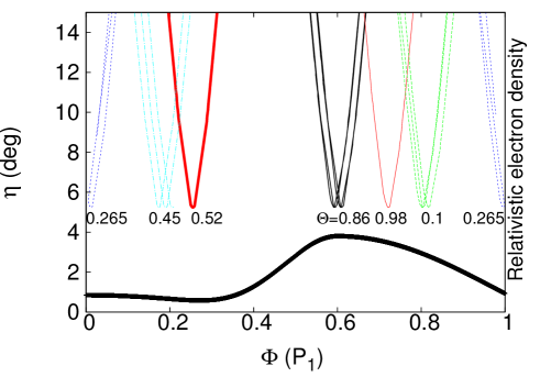
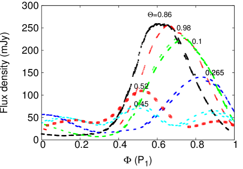
Figure 4: Top: The angle $\eta$ between jet axis and line of sight at different phases of the long-term modulation ($\Theta$) vs orbital phase ($\Phi$). One sees as the minimum of $\eta$, which corresponds to maximum Doppler boosting, moves at different $\Phi$s for the different $\Theta$ phases. The black thick curve is (on an arbitrary scale) the adopted relativistic electron density function of $P_{1}$ of Sect. 2.4. Bottom: Amplitude modulation and orbital shift of the outbursts: outbursts at different $\Theta$s vs $\Phi$ (with the same colour code as the above panel). The outburst decreases its amplitude and shifts in orbital phase.

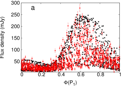
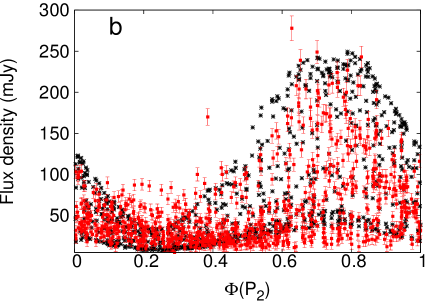
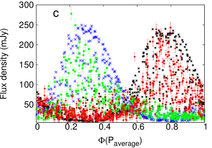
Figure 5: 8.3 GHz GBI observations (red squares) and model (black stars) data. All phases, $\Phi$, refer to $(t-t_{0})$, with $t_{0}$=JD2443366.775 (Gregory 2002). a): vs $\Phi$ ($P_{1}$) (orbit $P_{1}=1/\nu_{1}$=26.49 days); b): vs $\Phi$ ($P_{2}$) (precession $P_{2}=1/\nu_{2}$=26.92 days; c): 8.3 GHz GBI observations before (red points) and after (green points) 50841 MJD vs $\Phi$ ($P_{\rm average}$) ($P_{\rm average}=2/(\nu_{1}+\nu_{2})$=26.70 days). The points cluster separately with a shift of 0.5 in phase. The model reveals the same double clusterings: Black points refer to model data before 50841 MJD and blue points to model data after 50841 MJD.

.

4.2 Amplitude modulation and orbital shift of the outburst occurrence

During the maximum of the long-term modulation, the peak of the outburst occurs at orbital phase $\Phi\sim 0.6$ (Paredes et al. 1990). Afterwards, the orbital phase of the peak of the outburst changes, a phenomenon analysed in the past by Paredes et al. (1990, with references there) in terms of orbital phase shift, and by Gregory et al. (1999) in terms of timing residuals. In this section we show how our model of a precessing ($P_{2}$) jet with periodically ($P_{1}$) varying ejection reproduces i) the observed gradual shift of outburst occurrence from $\Phi=0.6$ to longer orbital phases ($\Phi\sim 0.9$) towards the minimum, ii) the so-called “quiet phase emission with no distictive maximum” discussed in Paredes et al. (1990), and iii) the observed re-appearing of outbursts having a distinctive maximum, even if still low, at orbital phase $\Phi\sim 0.5$.

Figures 3 c and 3 d discussed in the previous section show the variations of angle $\eta$ formed by the jet with the line of sight, vs orbital phase for the two extreme situations: $\Theta=0.83$ and $\Theta=0.52$, which is close to the maximum and the minimum of the long-term modulation. We now consider the curves of $\eta$ for several different $\Theta$ values (Fig. 4 top) and the related outbursts (Fig. 4 bottom).

At $\Theta$=0.86, the minimum of $\eta$ that corresponds to the maximum Doppler boosting occurs at $\Phi$=0.6. In the same Fig. 4 (top) the adopted relativistic electron density is drawn, as a function of $P_{1}$, with its maximum at $\Phi$=$\Phi_{r}$=0.6. Clearly at $\Theta$=0.86 the maximum Doppler boosting and the maximum ejection occur at the same orbital phase; that is, the electrons are ejected at the minimum $\eta$ angle with respect to the line of sight. After 200 days, at $\Theta$=0.98 the maximum Doppler boosting occurs at $\Phi$=0.7 (red curve at $\Theta$=0.98 in Fig. 4 top), and it matches the decay phase of the ejection. The result is the red dotted curve of Fig. 4 (bottom): an outburst slightly lower than that at $\Theta$=0.86 and shifted at $\Phi$=0.7. At $\Theta$=0.1 we can appreciate the evolution of the same phenomenon: the maximum Doppler boosting (MDB) (green curve in Fig. 4 top) is further shifted in phase and this causes a shifted and lower outburst (green curve in Fig. 4 bottom). In the interval starting after $\Theta$=0.265 (with the peak of the outburst at $\Phi\simeq 0.85$) until $\Theta\sim$0.45 , the outburst loses its typical shape, which is now a rather broad low outburst, and it becomes very difficult to define a peak (see the curve at $\Theta=0.45$ in Fig. 4 bottom). This is the so-called “quiet phase emission, with no distinctive maximum” noticed by Paredes et al. (1990) during the minimum of the long-term modulation. Finally, the outburst starts to resume its shape at $\Theta$=0.52. As one can see in Fig. 4, there is some boosting at the onset of the new ejection peaking at $\Phi=0.6$. The result is an outburst with peak at $\Phi\simeq 0.5$. Our model, therefore, is able to reproduce the orbital phase shift of Fig. 5 of Paredes et al. (1990).

4.3 Orbital and outburst periodicities

Figure  2 b, where the fits of two consecutive large outbursts are shown, has already proved the ability of the model also reproducing the shorter orbital periodicity, $P_{1}=26.49$ d. Here the comparison is extended to the whole data set, by folding, as shown in Fig. 5 a, all 6.7 yr of GBI data and model data with $P_{1}$. However, $P_{1}$ refers to the orbital periodical ejection of relativistic electrons, the real periodicity of the outburst is $P_{\rm average}=26.70$ d (Sect. 1). Because $P_{\rm average}$ is the average of $P_{1}$ and $P_{2},$ one would expect, when folding the data with $P_{\rm average}$, a clustering similar to or somehow intermediate to what is obtained using $P_{1}$ and $P_{2}$ (shown in Fig. 5 b). In contrast, Fig. 5 c reveals a double clustering. In Fig. 5 c, we use a different colour for model data and observations before or after the minimum of the long-term modulation. The GBI points before (red points) and after (green points) 50841 MJD cluster separately with a shift of 0.5 in phase. This effect is discussed in Massi & Jaron (2013) and Jaron & Massi (2013). What we want to point out here is that our model indeed reveals the same double clustering as the GBI observations: model data before (black points) and after (blue points) 50841 MJD cluster separately with a shift of 0.5 in phase as well.

Figure 6: Top: Spectral index $\alpha$ folded with the long-term modulation (phase $\Theta$) from GBI data at 2.2 GHz and 8.3 GHz (Massi & Kaufman Bernadó 2009). Bottom: $\alpha$ vs $\Theta$ from model data at 2.2 GHz and 8.3 GHz averaged over 4 days.

4.4 Spectral index

The top panel of Fig. 6 shows the observed spectral index, from GBI data at $\nu=2.2$ GHz and 8.3 GHz, folded with the 1667 d long-term modulation. The GBI data indicate that at some $\Theta$ phases, the emission in LS I +61^∘303 develops an optically thick spectrum ($\alpha\geq$ 0). This is the flat or inverted spectrum typical of jets in microquasars as discussed in Sect. 2.1. Our model of a precessing conical jet with a periodical increase in intrinsic emission must therefore be able to reproduce this spectral characteristic of LS I +61^∘303 emission.

To make the comparison, we calculated the observed flux, $S_{\rm model}$, at 2.2 GHz just by replacing this frequency in equations shown in Sect. 2 and using the parameters obtained by fitting the model to GBI data at 8.3 GHz, i.e. the set of parameters used to generate all figures. Indeed the model spectral index shown at the bottom of Fig. 6  is consistent with the observed one (Fig. 6 top). In particular, we note that the emission becomes optically thick at $\Theta$s where the maximum emission of relativistic electrons occurs at the smallest observing angles. In this case, in fact, high values of the optical depth are obtained and the emission becomes optically thick (see Sect.2.3). A deep analysis of the evolution of the opacity in the jet vs $\Phi$ and vs $\Theta$ is the argument of a paper in preparation. Whereas the model presented here consists of only a conical jet, the following paper will include the transient jet as well. In microquasars, the so-called transient jet always occurs after an optically thick phase (i.e., after the inverted/flat spectrum phase) and is associated to a large optically thin outburst (Fender et al. 2004; Massi 2011). In LS I +61^∘303 , the large optically thin outburst occurs about five days after the optical thick outburst and dominates at 2.2 GHz (Massi & Kaufman Bernadó 2009). The optically thin outburst suddenly reverses $\alpha$ from positive values to the low value $\alpha\simeq-0.5$, and this corresponds, as discussed in Massi & Kaufman Bernadó (2009, Sect. 5.1), to a new population of energetic electrons with an index power law p=2, which is steeper than the one associated to the conical jet, modelled here, with p=1.8. It is rather interesting that existing analyses of the origin of high energy emission in LS I +61^∘303 invoke not only two populations of electrons, but also populations with almost the same index as results from radio analysis (p=1.8 for the conical jet and p=2 for the transient jet). Zabalza et al. (2011) exclude GeV and TeV emission in LS I +61^∘303 being produced from the same parent particle population and determine an index $\leq 1.8$ for Fermi data and $2.1$ for MAGIC data.

4.5 VLBA maps vs model

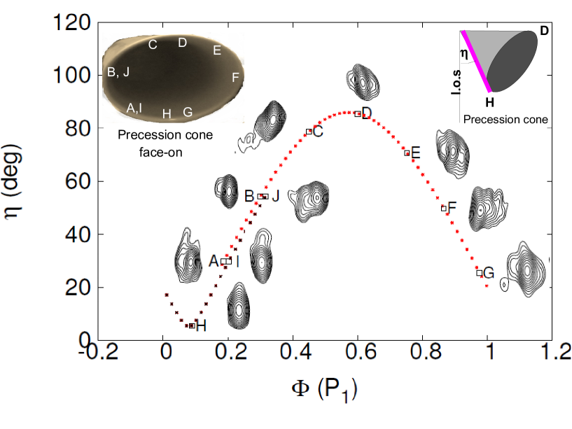
Figure 7: Angle $\eta$ between the jet axis and the line of sight at the epochs of the VLBA runs A-J. The trend of $\eta$ vs $\Phi(P_{1})$ is shown together with the VLBA maps (Massi et al. 2012) (see Sect. 4.5). The VLBA runs cover 30 days, then more than one orbital cycle of 26.49 days; runs I at $\Phi=0.203$ and J at $\Phi=0.316$ were performed one cycle later than runs A at $\Phi=0.187$ and B at $\Phi=0.30$. The shift of $\eta$ (corresponding to a shift of the maximum Doppler boosting) is already appreciable in Fig. 7 even after just one $P_{1}$ cycle; i.e., the two $\eta$ curves (black and red ones) vs $\Phi$ do not overlap.

Hints of a fast precessing jet in LS I +61^∘303 arose when two consecutive MERLIN images revealed a surprising variation of 60$\degr$ in position angle in only one day (Massi et al. 2004). A set of VLBA observations, A-J, interlapsed three days and covering an interval of 30 days were performed by Dhawan et al. (2006). The VLBA images, about 5 mas in size (therefore more than a factor 10 the orbital size, $2\times a=$0.45 mas) were showing highly varying features. With our model we can determine the variation in the ejection angle during the VLBA runs and compare these variations with the observed variations in position angle of the maps. The changes of $\eta$ are due to precession, but we put them as usual as a function of the orbit, that is of $\Phi(P_{1})$, and relate them to changes in VLBA maps also given as a function of $\Phi(P_{1})$ in Dhawan et al. (2006) and Massi et al. (2012). The trend of $\eta$ vs $\Phi(P_{1})$ is shown in Fig. 7 together with the high dynamic range VLBA images by Massi et al. (2012).

In Fig.7 we see, as the plot of $\eta$ vs $\Phi$ reveals, that run H was performed at the minimum $\eta,$ and D was performed nearly at the maximum $\eta$. These two extreme situations of $\eta$ for the two runs, H and D, are sketched in Fig.7 (right corner). This important information implies that two runs at similar $\eta$, but one performed before and the other after run D, refer to two jets pointing in opposite directions with respect to the axis of the precession cone (Fig. 7, left corner). If the model is correct, the position angle of the associated radio structures should reflect this different orientation. Indeed, the structure for run E points towards the SW, whereas runs C and J show structures pointing to SE. Similarly, the structure at run B points E, whereas that for run F points W. Finally, for A,I,H,G, our model results in a low $\eta$ angle, and this corresponds to a jet pointing closest to the earth. One can see that the related VLBA structures develop indeed a N-S feature. In run A (G), a transition of the geometry between B (F) and H,I is even traceable.

4.6 Derived jet parameters

The model fitting of Sect. 3 determines the values of two normalization factors present in our model, i.e. the normalization factor for the jet emission

$$Q={2x_{0}^{2}r_{0}J_{0}\over-(2-2\leavevmode\nobreak\ a_{3}-(p+2)a_{2})D^{2}},$$ (16)

and the normalization factor of the jet optical depth

$$q=(2.2\leavevmode\nobreak\ 10^{9})^{-(p+4)/2}{2\chi_{0}r_{0}\over-\kappa_{0}(2-2\leavevmode\nobreak\ a_{3}-(p+2)a_{2})}$$ (17)

where $r_{0}=x_{0}\leavevmode\nobreak\ \tan\leavevmode\nobreak\ \xi$.

Taking expressions (12) and (13) into account and assuming $p=1.8$ and $D=\leavevmode\nobreak\ 2.3\leavevmode\nobreak\$Kpc (Gregory et al. 1979), we can express the constant quantities $Q$ and $q$ in terms of the jet physical parameters

$$Q={x_{0}^{3}tg\xi\leavevmode\nobreak\ B_{0}^{1.4}A\over-(2-2\leavevmode\nobreak\ a_{3}-(p+2)a_{2})}4.4\times 10^{-50}$$ (18)

$$q={x_{0}tg\xi\leavevmode\nobreak\ B_{0}^{1.9}\over-(2-2\leavevmode\nobreak\ a_{3}-(p+2)a_{2})}3.8\times 10^{-3}$$ (19)

and derive, for the solution of Sect. 3, the values for the magnetic field intensity at the jet basis, $B_{0}$, and that for the normalization distance $x_{0}$:

$$B_{0}\simeq 9\leavevmode\nobreak\ \leavevmode\nobreak\ {\rm G}\leavevmode\nobreak\ \leavevmode\nobreak\ \leavevmode\nobreak\ \leavevmode\nobreak\ \leavevmode\nobreak\ \leavevmode\nobreak\ \leavevmode\nobreak\ \leavevmode\nobreak\ \leavevmode\nobreak\ x_{0}\simeq 1.6\leavevmode\nobreak\ 10^{13}{\rm cm}.$$

An independent estimate for the magnetic field strength is the value of the equipartition $B_{eq}\simeq 0.7\leavevmode\nobreak\$G derived from VLBI data (Massi et al. 1993) for a source size $d\simeq 5.5\leavevmode\nobreak\ 10^{13}$ cm, assuming equipartition between high energy particle energy and magnetic energy. To compare the result of $B_{0}\simeq 9\leavevmode\nobreak\$G for our model to $B_{eq}$, we compute the jet mean magnetic field $\tilde{B}$ over its length $L$. When considering the magnetic field functional form (Sect. 2.1), the topology resulting in Sect. 3 and the value of $L$ (Sect. 2.3), from the expression

$$\tilde{B}={B_{0}\over L}\int_{1}^{L}l^{-a_{2}}\leavevmode\nobreak\ dl,$$ (20)

we obtain $\tilde{B}\simeq 0.6\leavevmode\nobreak\$G, which is consistent with the value of $B_{eq}$ derived from the VLBI observation.

From the parameters deduced above, the electron energy content can also be estimated. Since synchrotron emission is centred on a peak spectral frequency $\nu$ (Ginzburg & Syrovatski 1965) such as

$$\nu=1.8\leavevmode\nobreak\ 10^{6}\gamma^{2}B,$$ (21)

the electron energy, $E=\gamma mc^{2}$, can be derived for different values of the magnetic field strength along the jet and for the two frequencies, $\nu=2.2\leavevmode\nobreak\ 10^{9}Hz\div 8.3\leavevmode\nobreak\ 10^{9}Hz$, considered in this analysis. At the jet basis (l=1), $B=B_{o}$, and $\gamma\simeq 11\div 22$ results. For the jet end (l=L), we must take both the decreased magnetic field intensity and relativistic electrons adiabatic losses into account (synchrotron losses are negligible) so that an electron with $\gamma(l=1)$ at the jet basis arrives at the jet end with $\gamma(L)=\gamma(1)L^{-2/3}$ (Kaiser 2006). To reproduce the observed emission for $\nu=2.2\leavevmode\nobreak\ 10^{9}Hz\div 8.3\leavevmode\nobreak\ 10^{9}Hz$ at the jet end, we need

$$\gamma(L)^{2}B(L)=\gamma(1)^{2}B_{o}L^{-2/3-2}=\nu/1.8\leavevmode\nobreak\ 10^{6},$$ (22)

i.e., for the solution of Sect.3, at least electrons with $\gamma(1)\simeq 371\div 741$.

In conclusion, relativistic electrons with energies in the range $10\leavevmode\nobreak\ mc^{2}\la E\la 740\leavevmode\nobreak\ mc^{2}$ are needed to reproduce the radio emission analysed in this paper. Since the mean over the orbital period of the adopted angular expression (the one shown in Fig. 4 top, see Sect.2.4 ) is $0.58\leavevmode\nobreak\ A$, the luminosity injected in the two jets in the form of relativistic electrons results in

$$L_{rel}=2(\pi r_{o}^{2}c)\leavevmode\nobreak\ 0.58A\int^{E_{Max}}_{E_{min}}E^{1-p}dE\simeq 5\leavevmode\nobreak\ 10^{34}\leavevmode\nobreak\ \leavevmode\nobreak\ {\rm ergs/sec}.$$ (23)

This value is only an indicative lower limit for the luminosity in the injected relativistic electron distribution since it is strictly related to the specific part of the radio spectrum analysed in this paper. In particular the presence of synchrotron emission at higher frequencies will imply higher values for electron energies and, consequently, higher values of $L_{rel}$. Indeed, jets from X-ray binaries are supposed to radiate from radio to optical wavelengths. The jet origin for the emission is supported by the correlation of the emission in the different bands (Russell et al. 2013, and reference therein). In this respect, it is worth noting that in LS I +61^∘303 the timing analysis of optical data by Zaitseva & Borisov (2003) results in a period equal to $P_{1}$. This result confirms what has previously been reported by Mendelson & Mazeh (1989, 1994) and Paredes et al. (1994). Particularly intriguing is that the light curve folded with this period shows that the brightness increases in the orbital phase interval where the radio outburst occurs. Finally, as already pointed out in Sect. 4.4, the present analysis holds true for the conical jet with p=1.8 considered here. Shocks in a transient jet may produce even more accelerated particles with a different energy power-law distribution.

4.7 The low/hard X-ray state

The varying morphology of VLBA images, plus the lack of accretion disk features (e.g., black body radiation) in the X-ray spectrum of LS I +61^∘303, have led some authors to favour non-accretion models (e.g., Dubus 2013). VLBA images were discussed in Sect. 4.5, and in this section we analyse the X-ray state of LS I +61^∘303. In fact, an accreting object presents rather different X-ray states (McClintock & Remillard 2006). While the requested black body component is the characteristic of the thermal state (McClintock & Remillard 2006), radio and X-ray observations of LS I +61^∘303 point towards a very low low/hard X-ray state.

As shown by Corbel et al. (2013), in the early phase of jet formation, the low density of particles in the jet produces an optically thin synchrotron power-law spectrum; as the density of the jet plasma increases, this leads to a transition to higher optical depth and to a flat/inverted radio spectrum ($\alpha\geq 0$). When sources having these self-absorbed compact radio jets are observed in X-rays, they reveal a low/hard X-ray state (Gallo et al. 2003; Fender et al. 2004). Concerning LS I +61^∘303, it is known that its persistent radio emission develops a flat/inverted radio spectrum at some orbital phases (exactly where an increased accretion is predicted) as shown by GBI observations at 2.2 GHz and 8.3 GHz (Massi & Kaufman Bernadó 2009). In addition, a flat spectrum has been recently observed by the Effelsberg 100-m telescope at four frequencies, from 4.85 GHz to 14.6 GHz (Fig. 4.13 Zimmermann (2013)).

Modelling of the low/hard state, especially at very low luminosities, favours an accretion disk truncated at a large radius (Fender 2001; Gardner & Done 2013, and references therein). The origin of the X-ray power-law emission with a typical photon index $\Gamma\sim 1.7$ (Remillard & McClintock 2006) (for LS I +61^∘303 in the range $1.5-1.8$, Sidoli et al. (2006); Chernyakova et al. (2006); Zimmermann & Massi (2012)) is still controversial, if it is due to a Comptonizing corona or/and to the jet (Markoff et al. 2001). Nevertheless, it is well established that this X-ray power-law emission that characterizes the low/hard state is correlated with the radio emission from the self-absorbed jet ($L_{R}\propto L_{X}^{0.7}$, Gallo et al. (2003)). The luminosity values for LS I +61^∘303 are $L_{X}=(1-6)10^{34}$ ergs/sec and $L_{R}=(1-17)\times 10^{31}$ ergs/sec (Combi et al. 2004). From Eqs. 3 and 5 in Merloni et al. (2003), we obtain

$$\xi_{RX}={{\rm log}L_{R}-\xi_{{\rm RM}}{\rm log}M-b_{\rm R}\over{\rm log}L_{X}}$$ (24)

where $\xi_{{\rm RM}}=0.69-0.89$ and $b_{\rm R}=3.26-11.38$ (Merloni et al. 2003). For a mass of 3 $M_{\odot}$ (where the influence of the mass difference between a neutron star of 1.4 $M_{\odot}$ and a stellar mass black hole of $3-15M_{\odot}$ is negligible in the result), we obtain $\xi_{RX}\leavevmode\nobreak\ =0.55-0.85$. This value is consistent with the solutions $\xi_{RX}=0.49-0.71$ by Merloni et al. (2003) and with the value of $\sim 0.7$ by Gallo et al. (2003) for accreting black holes in low/hard state, and it is clearly below the value $>1.4$ given by Migliari & Fender (2006) for accreting neutron stars in the low/hard state. Even though the nature of the compact object in LS I +61^∘303 is still unknown (Casares et al. 2005), the agreement with the low/hard state of black hole X-ray binaries would indeed favour the black hole scenario.

The luminosity for accreting black holes in the low/hard state is about $L_{\rm X}\sim 10^{36}\leavevmode\nobreak\ {\rm erg/sec}$ that may drop to $L_{\rm X}=10^{30.5}-10^{33.5}$ erg/s (McClintock & Remillard 2006) at the lowest phase, which is called the quiescent state. With its luminosity $L_{\rm X}=(1-6)10^{34}$ ergs/sec, LS I +61^∘303 is clearly in a very low low/hard X-ray state. That is a similar case to MWC 656, the recently discovered Be-black hole system, which is in the quiescent state (Casares et al. 2014). During the low-hard state the liberated energy of the accretion is thought to be converted into magnetic energy that powers the relativistic jet typically observed in this state (Smith 2012, and references therein). In a system in quiescence, Gallo et al. (2006) demonstrate that the outflow kinetic power accounts for a sizable fraction of the accretion energy budget.

5 Conclusions

In this paper we have developed a model that reproduces the observed long-term modulation of the radio emission of the binary system LS I +61^∘303 . The hypothesis is that the radio emission is due to a jet precessing with a period of $P_{2}=26.92\pm 0.07\,\mathrm{days}$. The jet is anchored on the accretion disk of a compact object orbiting, with a period of $P_{1}=26.49\pm 0.07\,\mathrm{days}$, the Be star. Variable accretion around the eccentric orbit increases the relativistic electron density in the jet at a particular orbital phase. We fitted our theoretically derived flux density, $S_{\rm model}(t)$ (see Eq. 1) to 6.5 yr GBI radio observations and determined the parameters of Table 1. We found that the precessing ($P_{2}$) jet model with intrinsic periodical variations ($P_{1}$) of emitting particles reproduces all seven observational facts:

1. the long-term modulation (Gregory 2002, and references there), see Fig. 2 a and Fig. 4 bottom;

2. the orbital shift of the peak of the radio outburst (Paredes et al. 1990), see Fig. 4 bottom;

3. the periodical outburst with orbital occurrence (Gregory 2002, and references there), see Figs. 2 b and c and Fig. 5 a;

4. the double clustering for data folded with $P_{1}+P_{2}\over 2$ (Massi & Jaron 2013), see Fig. 5 c;

5. the spectral index evolution (Massi & Kaufman Bernadó 2009), see Fig. 6;

6. a variation of the ejection angle suggestive of the rapid rotation in position angle of VLBA maps (Dhawan et al. 2006; Massi et al. 2012), see Fig. 7;

7. the strength of the magnetic field (Massi et al. 1993), see Sect. 4.6.

The maximum of the long-term modulation occurs when the maximum ejection of relativistic electrons takes place and at the same time the approaching jet is forming the smallest possible angle with the line of sight (i.e., the Doppler boosting is at its maximum). After a cycle of duration $P_{2}$, when the approaching jet again forms the smallest angle $\eta$, the ejection is now already on its decay phase (being $P_{1}<P_{2}$) and its Doppler boosting gives rise to an outburst with a lower amplitude than that of one cycle before. As we quantitatively show in Sect. 4.2, the peak of the outburst gets lower and lower at each cycle until the most unfavorable situation occurs, i.e., when the jet is pointing towards us while the main ejection is at its minimum. After this point, it happens that when the approaching jet again forms the smallest $\eta$ angle, there is the beginning of a new ejection of particles and the observed flux density slowly rises again. The period of 1667$\pm$8 days (Gregory 2002) of the long-term modulation is then just the number of $P_{1}$ cycles needed to compensate for the difference $P_{2}-P_{1}$ and synchronize $P_{1}$ again to $P_{2}$, which is just $[P_{2}/(P_{2}-P_{1})]P_{1}$ (Massi & Jaron 2013).

Our model, meant in the first instance to explain the long-term modulation affecting the radio emission of LS I +61^∘303, can become a powerful tool for understanding the physical processes at work in this gamma-ray binary. For this purpose the model should be extended to include internal shocks in the conical flow, i.e., the transient jet. As discussed in Sect. 4.4. the transient jet observed in LS I +61^∘303 is associated to a second population of relativistic electrons, with $p=2.0$, which is therefore different from the population with $p=1.8$, forming the conical jet analysed in this paper. It is quite interesting that two similar populations are invoked to explain emission in the TeV and GeV band (Zabalza et al. 2011). The important implications, if confirmed, are that the GeV emission is related to inverse Compton of the electrons of the conical jet and that the TeV emission is related to electrons of the transient jet.

This model, with conical jet and transient jet can be tested by fitting it to the radio spectral index data analysed in Massi & Kaufman Bernadó (2009). The theory of accretion in an eccentric orbit (Sect. 2.4) also predicts an ejection around periastron passage, along with the ejection at orbital phase $\Phi$=0.6 considered here (i.e., towards apoastron). By fitting the model to the radio spectral index data, one could verify if each of the two populations of electrons is generated twice along the orbit, i.e., that the transient jet occurs at periastron as well.

Indeed, at different epochs, emission towards apoastron (Albert et al. 2009) and periastron (Acciari et al. 2011) was detected by Cherenkov telescopes. Different Doppler boosting of the two ejections along the eccentric orbit could explain the observed variations. Maximum Doppler boosting occurring between the two ejections could explain the broad gamma-ray emission without any clear orbital modulation observed in Fermi-LAT data (Hadasch et al. 2012; Ackermann et al. 2013).

Finally, considering that one contribution to the gamma-ray emission consists of upscattered stellar photons, the role of Doppler boosting in gamma-ray emission is probably even more important than in the radio band. In fact, the amplification due to the Doppler factor for external inverse Compton is higher than for synchrotron emission (Kaufman Bernadó et al. 2002, and reference therein).

Appendix A Optical depth through a stratified jet

The integration upper limit in the intensity expression in Eq.(7), $\tau_{end}(l)$, represents the jet’s maximum optical depth. Figure A1 shows a cut of the jet structure where the line of sight makes an angle $\eta$ with the jet axis, $l$. When looking at the figure it is easy to understand how photons coming out from the jet side facing the observer at generic distance $x_{0}l$ originate along the integration path inside the jet, i.e., along the segment AB for the case of the approaching jet shown in the figure.

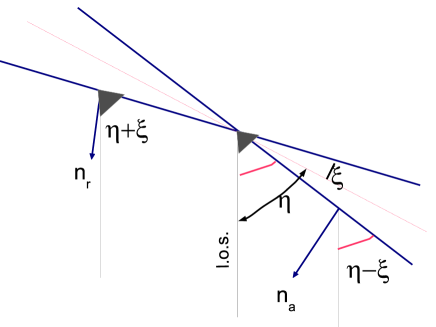
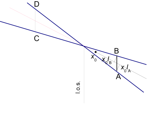
Figure 8: Top: Perpendicular directions (n) to the surfaces facing the line of sight (l.o.s.) of the approaching and receding components of a jet with aperture $\xi$ and an angle $\eta$ with respect to the line of sight. Bottom: Optical path through the two jet components (see text).

If we call $l_{A}$ the value of the axial distance corresponding to point $A$ and $l_{B}$ that corresponding to point $B$, the following relationships describe the geometrical projection of the optical path $AB$ on the jet axis and on the jet radius, respectively:

$$AB\leavevmode\nobreak\ \cos\leavevmode\nobreak\ \eta=x_{0}\leavevmode\nobreak\ (l_{A}-l_{B})$$ (25)

$$AB\leavevmode\nobreak\ \sin\leavevmode\nobreak\ \eta=r(l_{A})+r(l_{B})=r_{0}\leavevmode\nobreak\ (l_{A}+l_{B})$$ (26)

The jet region included between $l_{A}$ and $l_{B}$, i.e., $l_{A}\geq l\geq l_{B}$, is the one that contributes to the emission coming out of the jet at $l=l_{A}$. It is evident from the figure that the emitting region is different for different values of $l_{A}$. To quantify the depth of the involved region, the value of $l_{B}$ can easily be derived from the above expressions and results in

$$l_{B}=l_{A}\leavevmode\nobreak\ {\tan\leavevmode\nobreak\ \eta-\tan\leavevmode\nobreak\ \xi\over\tan\leavevmode\nobreak\ \eta+\tan\leavevmode\nobreak\ \xi}$$ (27)

All the above relationships hold in the limit that the angle $\eta$, between the jet axis and the line of sight, is larger than the jet opening angle $\xi=r_{0}/x_{o}$; i.e., $\tan\leavevmode\nobreak\ \eta>\tan\leavevmode\nobreak\ \xi$.

Once $l_{B}$ is known following Eq.(8), the optical depth at the distance $l_{A}$ is

$$\tau_{A}-\tau_{B}=-\int^{l_{A}}_{l_{B}}\chi_{\nu}\leavevmode\nobreak\ {\rm d}x=\leavevmode\nobreak\ \tau_{0}l_{A}^{\leavevmode\nobreak\ C}\leavevmode\nobreak\ [1-(l_{B}/l_{A})^{\leavevmode\nobreak\ C}]$$ (28)

where $C=1-a_{3}-(p+2)a_{2}/2$ and $\tau_{A}=0$ assuming no emission or absorbtion between the observer and the jet.

Since $l_{A}$ represents our generic distance along the jet axis, we can define for the approaching jet the optical depth $\tau_{end}\equiv\tau_{B}$ as

$$[\tau_{\rm end}]_{\rm app}(l)=\tau_{0}l^{\leavevmode\nobreak\ C}\leavevmode\nobreak\ \large\left[\large\left({\tan\leavevmode\nobreak\ \eta-\tan\leavevmode\nobreak\ \xi\over\tan\leavevmode\nobreak\ \eta+\tan\leavevmode\nobreak\ \xi}\large\right)^{\leavevmode\nobreak\ C}-1\large\right].$$ (29)

For the receding jet the same procedure can be performed by paying attention to some different signs (note that also for the receding jet the positive direction for $l$ is defined going away from the core), to arrive at

$$[\tau_{\rm end}]_{\rm rec}(l)=\tau_{0}l^{\leavevmode\nobreak\ C}\leavevmode\nobreak\ \large\left[1-\large\left({\tan\leavevmode\nobreak\ \eta+\tan\leavevmode\nobreak\ \xi\over\tan\leavevmode\nobreak\ \eta-\tan\leavevmode\nobreak\ \xi}\large\right)^{\leavevmode\nobreak\ C}\large\right].$$ (30)