Spatio-temporal dynamics of an active, polar, viscoelastic ring

Abstract

Constitutive equations for a one-dimensional, active, polar, viscoelastic liquid are derived by treating the strain field as a slow hydrodynamic variable. Taking into account the couplings between strain and polarity allowed by symmetry, the hydrodynamics of an active, polar, viscoelastic body include an evolution equation for the polarity field that generalizes the damped Kuramoto-Sivashinsky equation. Beyond thresholds of the active coupling coefficients between the polarity and the stress or the strain rate, bifurcations of the homogeneous state lead first to stationary waves, then to propagating waves of the strain, stress and polarity fields. I argue that these results are relevant to living matter, and may explain rotating actomyosin rings in cells and mechanical waves in epithelial cell monolayers.

1 Introduction

At molecular scales, the mechanics and self-organization of the cytoskeleton are driven by a chemical fuel, through ATP or GTP hydrolysis, and rely on the enzymatic activity of molecular motors to turn chemical energy into forces and motion. Numerous phenomena pertaining to cell division, cell motility, cell adhesion, or more generally pattern formation at the scale of the cytoskeleton, have been interpreted within the framework of hydrodynamics, where continuous fields subsume the behaviour of many individual active units, and governing equations are constrained by symmetry Juelicher2007 ; Ramaswamy2010 ; Marchetti2013 . Since biofilaments such as filamentous actin and microtubules are polar, orientational order must be considered. Cell rheology is characterized by a weak power-law frequency dependence of the response functions and by nonlinear behaviour, such as strain-stiffening Chen2010 . These complex features are difficult to treat analytically, rendering simpler rheologies all the more attractive to the theorist. The behaviour of active polar liquids has been studied in great detail Kruse2004 ; Kruse2005 ; Muhuri2007 ; Giomi2008 , while recent work has also dealt with the mechanical and dynamical properties of isotropic active solids Banerjee2011 ; Edwards2011 ; Yoshinaga2012 , and of active polar permeating gels Callan-Jones2011 .

Motivated by the observation of graded and alternating polarity profiles of filamentous actin in the actomyosin bundles of metazoan cells Yoshinaga2010 , we studied pattern formation in an active polar solid band, taking into account possible couplings between strain and polarity. We showed that the dynamics of the polarity field is governed by a damped Kuramoto-Sivashinsky equation Manneville1988 . For large damping, we found that an activity-driven stationary bifurcation leads to periodic patterns, suggesting a scenario for the emergence of sarcomeric organization in actomyosin bundles.

Here I treat the case of an active, polar, viscoelastic (Maxwell) liquid in one spatial dimension, considering the strain field as a hydrodynamic variable Brand1990 . For simplicity, the dynamical equations are studied analytically on an infinite line, and numerically with periodic boundary conditions: this study pertains to dynamical behaviour on a ring, or far from the boundaries in a quasi-one-dimensional system. One objective is to elaborate on the relevance of the damped Kuramoto-Sivashinsky equation to the dynamics of active polar materials. A study of the complete parameter space is beyond the scope of this work, where I show representative examples of the dynamics.

This article is organized as follows. In section 2, I derive the set of coupled evolution equations for the velocity, strain and polarity fields that govern the dynamics of an active polar viscoelastic liquid in one spatial dimension. In section 3, I perform the linear stability analysis of the homogeneous state, uncovering an activity-driven stationary bifurcation, then show numerically that propagating waves also arise farther from the bifurcation threshold. As summarized in the Appendix, I performed the same analysis in the case of an active, polar, viscoelastic (Kelvin) solid, and obtained similar results. In section 4, I discuss applications to living matter, at the scale of the cell with actomyosin bundles and rings, but also at the scale of the tissue with epithelial cell monolayers.

2 Constitutive equations

In this section, I derive constitutive equations for an active, polar, viscoelastic liquid in one spatial dimension. The relevant fields include the pressure $P$, the temperature $T$, the total stress $\sigma$, the strain $e$, the velocity $v$ and the polarity $p$, all dependent upon the spatial and temporal coordinates $(x,t)$. I derive constitutive equations expressing first the material’s free energy density as a Landau expansion around the zero strain, zero polarity homogeneous state, second the entropy production rate density as a function of the relevant thermodynamic force-flux pairs, and finally fluxes as a function of forces, including coupling terms allowed by symmetry Chaikin1995 .

The free energy density, expanded to quadratic order about $p=e=0$, reads

$$f=\frac{a}{2}\;p^{2}+\frac{K}{2}\;\left(\partial_{x}p\right)^{2}+\frac{G}{2}\;e^{2}+w\;e\;\partial_{x}p$$ (1)

where all terms are invariant under simultaneous inversion of space and polarity, and the polar term $\partial_{x}p$ is omitted since its contribution is equal to zero for periodic boundary conditions. The positive coefficients $a$, $K$, and $G$ respectively denote the susceptibility, the energy cost of inhomogeneities of the polarity field, and the elastic modulus. Symmetries of the problem allow for a coupling term between strain and polarity gradient, with a coupling parameter $w$ of arbitrary sign. Thermodynamic stability imposes the constraint $w^{2}\leq KG$. Differentiating eq. (1) yields the molecular field $h$, conjugate to the polarity

$$h=-\frac{\delta f}{\delta p}=-\;a\;p+K\;\partial^{2}_{x}p+w\;\partial_{x}e$$ (2)

and the elastic stress, conjugate to the strain

$$\sigma^{\mathrm{el}}=\frac{\delta f}{\delta e}=G\;e+w\;\partial_{x}p.$$ (3)

As was first advocated in Brand1990 in the context of the viscoelastic relaxation of the transient (but long-lived) strain of polymer melts, I treat the strain field as an additional slow, hydrodynamic variable. The same approach was used recently to derive in a natural and rigorous manner the constitutive equations of active polar permeating gels Callan-Jones2011 . The density $R/T$ of the entropy production rate is obtained by standard manipulations of the conservation equations:

$$R=\left(\sigma+P\right)\;\partial_{x}v-\dot{e}\;\sigma^{\mathrm{el}}+\dot{p}\;h+r\;\Delta\mu.$$ (4)

This expression contains two mechanical terms, a polar term, and a (chemical) active term where the generalized force $\Delta\mu$ (variation of chemical potential due to ATP hydrolysis) is conjugate to the ATP consumption rate $r$. A dot denotes the total derivative, as in $\dot{p}=\partial_{t}p+v\,\partial_{x}p$. The conjugate flux-force pairs are

$$\mathrm{Flux} \leftrightarrow \mathrm{Force}$$

$$\sigma+P \leftrightarrow \partial_{x}v$$

$$\dot{e} \leftrightarrow \sigma^{\mathrm{el}}$$ (5)

$$\dot{p} \leftrightarrow h$$

$$r \leftrightarrow \Delta\mu.$$

Following a standard procedure Juelicher2007 ; Kruse2005 ; Callan-Jones2011 , the constitutive equations read

$$\sigma+P = \eta\;\partial_{x}v+\sigma^{\mathrm{el}}+\sigma_{\mathrm{a}}+\beta_{\mathrm{a}}\;\partial_{x}p$$ (6)

$$\dot{e} = \partial_{x}v-\Gamma_{e}\;\sigma^{\mathrm{el}}+{\dot{e}}_{\mathrm{a}}-\psi_{\mathrm{a}}\;\partial_{x}p$$ (7)

$$\dot{p} = \Gamma_{\mathrm{p}}\;h-\alpha_{\mathrm{a}}\;p\,\partial_{x}p-\lambda\;p\,\partial_{x}v$$ (8)

omitting the equation expressing as a function of thermodynamic forces the field $r$. The dynamic viscosity $\eta$ and the kinetic coefficients $\Gamma_{e}$ and $\Gamma_{\mathrm{p}}$ are positive. Active coupling coefficients are denoted by the index $a$, and are proportional to $\Delta\mu$, as in $\beta_{\mathrm{a}}=\beta\,\Delta\mu$. The active stress $\sigma_{\mathrm{a}}$ is positive for a contractile material. The invariance properties of polar media allow for an active coupling between stress and polarity gradient, with a coefficient $\beta_{\mathrm{a}}$, as first introduced in Giomi2008 . The active coefficients ${\dot{e}}_{\mathrm{a}}$ and $\psi_{\mathrm{a}}$ in eq. (7) play the same role as $\sigma_{\mathrm{a}}$ and $\beta_{\mathrm{a}}$ in eq. (6). Two advection terms with coupling coefficients $\alpha_{\mathrm{a}}$ and $\lambda$, of arbitrary signs, are included in eq. (8), in agreement with earlier studies of active liquid crystals Muhuri2007 ; Giomi2008 . Except for $\sigma_{\mathrm{a}}$ and ${\dot{e}}_{\mathrm{a}}$, the active terms in (6-8) contain products of $\Delta\mu$ with $p$ and its gradients, and are therefore stricto sensu nonlinear terms. In the long time limit, a non-zero value of ${\dot{e}}_{\mathrm{a}}$ would lead to unbounded values of the strain, unphysical in the regime of small deformations considered here. In the following, I therefore set ${\dot{e}}_{\mathrm{a}}=0$.

Three relaxation times characterize this material: the viscoelastic time $\tau=\eta/G$, the strain relaxation time $\tau_{\mathrm{e}}=(G\Gamma_{e})^{-1}$, and the polarity relaxation time $\tau_{\mathrm{p}}=(a\Gamma_{\mathrm{p}})^{-1}$. A separation of time scales may lead to distinct dynamical regimes since the viscoelastic time, the strain relaxation time and the polarity relaxation time may differ. Assuming a constant pressure and a constant active stress, the momentum conservation equation $\partial_{x}\sigma=0$ yields $\tau\;\partial^{2}_{x}v+\partial_{x}e+l_{\mathrm{p}}\;\partial^{2}_{x}p=0$, where $l_{\mathrm{p}}=\frac{w+\beta_{\mathrm{a}}}{G}$ is a length scale that characterizes the coupling between strain and polarity gradient. Anticipating the possibility of an instability of the homogeneous state $v=e=p=0$ at short wavelengths Yoshinaga2010 , I introduce a stabilizing higher-order polarity gradient term $\frac{\nu}{2}\,\left(\partial^{2}_{x}p\right)^{2}$ in the free energy density, where $\nu$ is a positive coefficient Chaikin1995 . As a consequence, the conjugate field $h$, eq. (2), is supplemented with the term $-\nu\;\partial^{4}_{x}p$. Altogether, the dynamics is governed by a set of three coupled partial differential equations

$$0 = \tau\;\partial^{2}_{x}v+\partial_{x}e+l_{\mathrm{p}}\;\partial^{2}_{x}p$$ (9)

$$\partial_{t}e+v\,\partial_{x}e = -\frac{1}{\tau_{\mathrm{e}}}e+\partial_{x}v-v_{\mathrm{p}}\,\partial_{x}p$$ (10)

$$\partial_{t}p+v\,\partial_{x}p+\lambda\;p\,\partial_{x}v+\alpha_{\mathrm{a}}\;p\,\partial_{x}p = -\frac{1}{\tau_{\mathrm{p}}}p+\Gamma_{\mathrm{p}}\left(K\,\partial_{x}^{2}p-\nu\,\partial^{4}_{x}p+w\,\partial_{x}e\right)$$ (11)

where $v_{\mathrm{p}}=\psi_{\mathrm{a}}+\Gamma_{e}w$ is a coefficient of arbitrary sign which characterizes the coupling between strain rate and polarity.

Given the definition (3) of the elastic stress $\sigma_{\mathrm{el}}$, its evolution equation is obtained by combining Eqs. (10) and (11):

$${\dot{\sigma}_{\mathrm{el}}}+\frac{\sigma_{\mathrm{el}}}{\tau_{\mathrm{e}}}=G\;\partial_{x}v+\left(\frac{w}{\tau_{\mathrm{e}}}-Gv_{\mathrm{p}}\right)\,\partial_{x}p+w\,\partial_{x}{\dot{p}}.$$ (12)

When the time $t$ is long compared to $\tau_{\mathrm{e}}$ and $\tau_{\mathrm{p}}$, ${\dot{\sigma}_{\mathrm{el}}}$ and ${\dot{p}}$ may relax to zero. In this limit, the elastic stress becomes a linear combination of the velocity and polarity gradients $\sigma_{\mathrm{el}}^{\infty}\to G\tau_{\mathrm{e}}\;\partial_{x}v^{\infty}+\left(w-G\tau_{\mathrm{e}}v_{\mathrm{p}}\right)\,\partial_{x}p^{\infty}$, and a stationary solution $\sigma^{\infty}(x)$ for the total stress reads (see eq. (6):

$$\sigma^{\infty}(x)=-P+\left(\eta+G\tau_{\mathrm{e}}\right)\partial_{x}v^{\infty}+\sigma_{\mathrm{a}}+\left(\beta_{\mathrm{a}}+w-G\tau_{\mathrm{e}}v_{\mathrm{p}}\right)\partial_{x}p^{\infty}.$$ (13)

Assuming that this stationary solution is stable, the constitutive equation for the stress field (13) is that of an active, polar liquid in the long time limit, as expected for a Maxwell viscoelastic liquid.

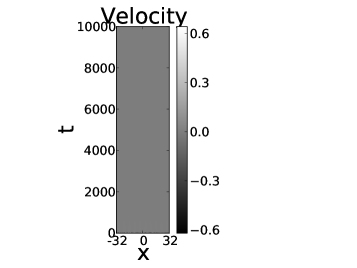
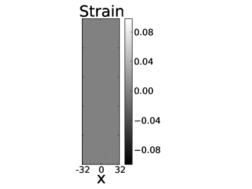
(a)
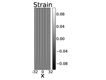
(b)
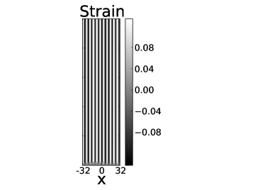
(c)

Figure 1: Stationary bifurcation. Numerical simulations of eqs. (9-11) were performed with XMDS2 Dennis2013 , with random initial conditions and periodic boundary conditions. The parameter values are: $a=1$, $K=1$, $w=1$, $\tau=\tau_{\mathrm{e}}=\tau_{\mathrm{p}}=1$, $v_{\mathrm{p}}=0$, $\lambda=1$, $\alpha_{\mathrm{a}}=2$, $\Gamma_{\mathrm{p}}=1$, $\nu=1$, leading to a threshold $l_{\mathrm{p}}^{c}=6$, see eq. (14). Space-time plots of the velocity, strain and polarity fields are given for $l_{\mathrm{p}}=5.99$ (a); $l_{\mathrm{p}}=6.01$ (b); $l_{\mathrm{p}}=6.1$ (c).

3 Instabilities

3.1 Stationary bifurcation

Harmonic perturbations of amplitude $(v_{0},e_{0},p_{0})$ to the reference homogeneous state read $(v,e,p)=(v_{0},e_{0},p_{0})\;e^{s(q)t-iqx}$, defining the growth rate $s(q)$ at wavenumber $q$. To linear order in the amplitudes $(v_{0},e_{0},p_{0})$, eq. (10) allows to eliminate the velocity ($v_{0}=v_{\mathrm{p}}p_{0}+\frac{i}{q}(s+\frac{1}{\tau_{\mathrm{e}}})e_{0}$), and to obtain a system of two linear equations in the unknowns $(e_{0},p_{0})$. Cancelation of the determinant yields a second-order polynomial equation $s^{2}+Bs+C=0$ for the growth rate. Since the coefficient $B(q^{2})=\frac{1}{\tau}+\frac{1}{\tau_{\mathrm{e}}}+\frac{1}{\tau_{\mathrm{p}}}+\Gamma_{\mathrm{p}}(K+\nu q^{2})\,q^{2}$ is always positive, complex solutions for the growth rate are always damped: linear stability analysis of the homogeneous state precludes oscillatory instabilities.

However, the coefficient $C(q^{2})=\left(\frac{1}{\tau}+\frac{1}{\tau_{\mathrm{e}}}\right)\frac{1}{\tau_{\mathrm{p}}}+\Gamma_{\mathrm{p}}\left[K\left(\frac{1}{\tau}+\frac{1}{\tau_{\mathrm{e}}}\right)-w\left(v_{\mathrm{p}}+\frac{l_{\mathrm{p}}}{\tau}\right)\right]\,q^{2}+\Gamma_{\mathrm{p}}\nu\left(\frac{1}{\tau}+\frac{1}{\tau_{\mathrm{e}}}\right)\,q^{4}$ may change sign, and a stationary instability occurs close to wavenumbers such that $C(q^{2})<0$, with a growth rate $s_{+}=(-B+\sqrt{B^{2}-4C})/2>0$. A straightforward calculation gives the instability threshold:

$$w\left(l_{\mathrm{p}}+v_{\mathrm{p}}\tau\right)>\left(1+\frac{\tau}{\tau_{\mathrm{e}}}\right)\left(K+2\sqrt{\nu a}\right)$$ (14)

or equivalently

$$w\left(\beta_{\mathrm{a}}+\eta\psi_{\mathrm{a}}\right)>(1+\Gamma_{\mathrm{e}}\eta)\,(KG-w^{2}+2G\sqrt{\nu a}).$$ (15)

Since $\eta\geq 0$, $\Gamma_{\mathrm{e}}\geq 0$, $G\geq 0$ and $w^{2}\leq KG$, the r.h.s. of eq. (15) is positive: the bifurcation is made possible by the presence of active, polar couplings. The fastest growing wavenumber is given by the solution $q_{0}$ of $\frac{\mathrm{d}C}{\mathrm{d}q^{2}}_{|q^{2}=q_{0}^{2}}=0$, from which the wavelength $\lambda_{0}=2\pi/q_{0}$ observed immediately beyond threshold is calculated

$$\lambda_{0}=2\pi\,\left[\frac{1}{2G\nu}\left(w^{2}-KG+w\,\frac{\beta_{\mathrm{a}}+\eta\psi_{\mathrm{a}}}{1+\Gamma_{\mathrm{e}}\eta}\right)\right]^{-\frac{1}{2}}\,.$$ (16)

This expression reduces to eq. (26) in the limit $\Gamma_{\mathrm{e}}\to 0$, $\psi_{\mathrm{a}}\to 0$.

The results of the linear stability analysis are confirmed by numerical simulations Dennis2013 of the full nonlinear system eqs. (9-11), supplemented for simplicity by random initial conditions, and by periodic boundary conditions (see figure 1). Although one expects a Maxwellian material to be liquid at times long compared to the viscoelastic time $\tau$, the strain field does not relax to zero, and exhibits a stationary, spatially periodic pattern of non-zero amplitude, due to the bifurcation made possible by active, polar couplings. Since the instability occurs in the bulk, these observations should be relevant far from the boundaries independently of specific boundary conditions Yoshinaga2010 .

3.2 Propagating waves

The damped (or stabilized) Kuramoto-Sivashinsky equation captures the universal features of numerous pattern-forming systems Manneville1988 ; Misbah1994 , such as directional solidification or liquid column flow Manneville1988 ; Brunet2007 . In one spatial dimension, it reads

$$\partial_{t}\phi+\phi\,\partial_{x}\phi=-\delta\,\phi-\partial_{x}^{2}\phi-\partial_{x}^{4}\phi.$$ (17)

where $\phi(x,t)$ denotes the relevant field, and $\delta$ is a positive damping coefficient. Large wavenumbers, destabilized by negative diffusion, are stabilized by the fourth-order spatial derivative. The advection term $\phi\,\partial_{x}\phi$ is responsible for energy transfer from small to large wavenumbers. With $\phi=\phi_{0}\;e^{s(q)t-iqx}$, the growth rate $s(q)$ at wavenumber $q$ is $s(q)=-\delta+q^{2}-q^{4}$: a stationary bifurcation occurs for $\delta\leq\delta_{c}=\frac{1}{4}$, with a most unstable wavenumber $q_{0}^{2}=\frac{1}{2}$. The aspect ratio is defined as the ratio between the system size and the wavelength $\lambda_{0}=2\pi/q_{0}$. For large aspect ratio, decreasing the (positive) damping coefficient leads through a cascade of bifurcations to a regime of spatio-temporal chaos: the Kuramoto-Sivashinsky equation is recovered in the limit $\delta\to 0$. Secondary and higher-order instabilities of eq. (17) were studied for small and intermediate aspect ratios in Misbah1994 and Brunet2007 respectively.

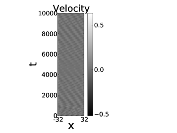
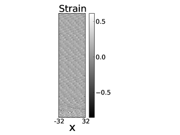
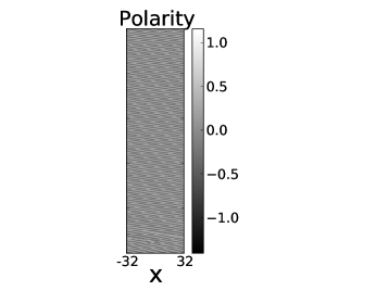
Figure 2: Propagating waves. Numerical simulations of eqs. (9-11) were performed with XMDS2 Dennis2013 , with periodic boundary conditions, and periodic initial conditions, eqs. (18) with $k=0.5$ and $\varphi_{0}=0.5$. The parameter values are: $a=1$, $K=1$, $w=1$, $\tau=\tau_{\mathrm{e}}=10$, $v_{\mathrm{p}}=0$, $\lambda=1$, $\alpha_{\mathrm{a}}=2$, $\Gamma_{\mathrm{p}}=0.1$ ($\tau_{\mathrm{p}}=10$), $\nu=1$, Space-time plots of the velocity, strain and polarity fields are given for $l_{\mathrm{p}}=4.5$, larger than the threshold value $l_{\mathrm{p}}^{c}=3.26$, see eq. (14).

Since eq.(11) generalizes the damped Kuramoto-Sivashinsky equation by additional couplings with the velocity and strain fields, I conjecture that their spatio-temporal dynamics contains that of the simpler system, eq. (17). Motivated by experiments (see section 4), I use numerical simulations to confirm the existence of higher-order bifurcations of the homogeneous solution of eqs. (9-11) to propagating waves. Following Brunet2007 , appropriate initial conditions read

$$p(x,t=0) = \sin(kx)+0.5\,\sin(2kx+\varphi_{0})$$

$$e(x,t=0) = 0$$ (18)

$$v(x,t=0) = -\frac{l_{\mathrm{p}}}{\tau}\,p(x,t=0)$$

where $k$ and $\varphi_{0}$ are a wavenumber and phase. As shown in figure 2, propagating waves are observed in numerical simulations of the system (9-11) with initial conditions (18) and periodic boundary conditions (see figure 4 for propagating waves similarly obtained for an active, polar, viscoelastic solid). In this active, polar viscoelastic liquid, the strain field does not relax to zero for times large compared to the viscoelastic time $\tau$, but adopts the same patterns as the polarity and velocity fields to which it is coupled.

4 Relevance to living matter

The above analysis is based on the invariance properties of active polar materials. In sections 4.1 and 4.2, I respectively discuss possible applications to the spatio-temporal dynamics of living matter obeying the same symmetries, first to the actin cytoskeleton, then to cohesive assemblies of collectively migrating cells. In all cases, validating the model necessitates a detailed comparison with experimental data that is left for future study.

4.1 Actomyosin bundles

A hydrodynamic description of the actin cytoskeleton requires length scales large compared to the mesh size of the polymer network. Actin filaments are polar: the hydrodynamic polarity field is naturally defined as a local, coarse-grained average of the polarity of individual actin filaments. Bundling is mediated by cross-linkers, either active or passive, also responsible for most of the bundle’s elasticity Yoshinaga2012 . A coupling between polarity and strain may arise given a preference of cross-linkers to parallel or anti-parallel pairs of actin filaments Meyer1990 . In the context of the actin cytoskeleton, polarity advection is naturally interpreted as expressing the transport of polarity due to faster polymerization at the barbed ends of actin filaments. Strain relaxes thanks to, e.g., crosslinker unbinding.

A stationary bifurcation is a likely scenario to explain the existence of monotonic (graded) and periodic (alternating) polarity patterns in actomyosin bundles Cramer1997 , that may self-organize into sarcomeres for large enough active couplings. I show here that this bifurcation occurs whether the bundle rheology is that of a viscoelastic liquid or that of a viscoelastic solid, suggesting that the proposed mechanism does not depend on a specific rheology. Assuming that myosins (resp. $\alpha$-actinins) concentrate close to the barbed (resp. pointed) ends of actin filaments, the same mechanism may also explain, with the same wavelength, the banded patterns seen in the distribution of myosin and $\alpha$-actinin along stress fibers Peterson2004 and apical circumferential bundles Ebrahim2013 . The wavelength of polarity patterns depends on the value of active couplings (see eqs. (16) and (26)): a prediction of the model is that down- or up-regulating contractility should modify the typical length of a sarcomere. Indeed, this has been observed experimentally Peterson2004 .

Cells spread on a flat substrate assemble ring-like, contractile bundles around their nucleus Senju2009 . Another prediction is that actomyosin rings may spontaneously rotate, due to the occurrence of propagating waves in an active, polar, viscoelastic ring (see figures 2 and 4). As a consequence of mechanical coupling between the actin cytoskeleton and the cell nucleus, rotation of the actin ring may in turn entrain the rotation of the cell nucleus Kumar2014 . Another active, polar, viscoelastic ring is the contractile ring assembled during cytokinesis by eukaryotic cells Eggert2006 : it may also rotate thanks to the same mechanism.

In Asano2009 , a propagating wave observed at the periphery of a spread, adhering cell under inhibition of Rac-mediated lamellipodial formation was interpreted as an actin density wave resulting from the active couplings of the polarity and concentration fields, in the limit of zero velocity in the actin cytoskeleton. The model proposed here generalizes this result to a viscoelastic material with arbitrary strain and velocity.

4.2 Collective cell migration

Hydrodynamic descriptions of tissues are possible for length scales large compared to a typical cell size. Motile cells are polar entities, with a well-defined front and rear. A cohesive assembly of cells migrating collectively Ilina2009 ; Roerth2012 may for this reason be described as an active polar material Koepf2013 , where the coarse-grained polarity may arise from the rear-front polarity of individual cells Farooqui2005 , or from the position of the centrosome with respect to the cell nucleus Reffay2011 . In Xenopus mesendoderm cells, force application through cadherin-mediated adhesions leads to protrusive activity at the opposite side of the cell, and to collective cell migration Weber2011 . This coupling between cell-cell adhesion and polarity (see also desai2009 ) leads to a possible interpretation of the coefficient $w$. A recent study relates strain relaxation in tissues to cell division and apoptosis Ranft2010 .

Collective migration has been studied in vitro in epithelial cell monolayers at confluence, with a recent report of propagating mechanical waves during tissue expansion Serra-Picamal2012 . Interestingly, the wave velocity is distinct from the spreading velocity of the epithelium boundary, and the phenomenon is suppressed when inhibiting contractility: these observations are consistent with the mechanism proposed here for propagating mechanical waves in an active, polar, viscoelastic medium. Note that the model admits propagating waves for an aspect ratio as small as $2$ (not shown), as observed in the experiment, albeit for different (free) boundary conditions Serra-Picamal2012 .

Strikingly, global tissue rotation appears to be a generic feature of epithelial cells (see Roerth2012 for a review), perhaps calling for a simple physical explanation such as the one proposed here. An in vivo example is the rotation of the follicular epithelium of Drosophila eggs, contributing to the elongation of the egg Bilder2012 . In vitro, cell monolayers were found to rotate spontaneously on ring-shaped micro-patterned surfaces Wan2011 . Whether cultured on a flat substrate Brangwynne2000 , or in a three-dimensional gel Tanner2012 cell assemblies engage in coherent angular motion for cell numbers as small as two, in which case a hydrodynamic description, if applicable, would be likely to pertain to cytoskeletal rather than epithelial mechanics.

5 Conclusion

Due to instabilities of the homogeneous state, the space-time dynamics of an active, polar, viscoelastic liquid in one dimension of space includes stationary and propagating waves. On a ring, the propagation of mechanical and polarity waves is tantamount to spontaneous rotation. Beyond the threshold of the linear instability, the strain field remains relevant for times long compared to the viscoelastic time: the strain amplitude no longer relaxes to zero. Necessary ingredients for pattern formation are a polarity advection term $p\,\frac{\partial p}{\partial x}$, as well as non-zero coupling terms between polarity gradients and the mechanical fields. The advection term arises due to symmetry in hydrodynamic models of self-propelled systems Toner2005 , and has been explicitly derived from a microscopic model of the interaction of actin filaments with molecular motors Ahmadi2006 . Denoting $w$, $\beta_{\mathrm{a}}$ and $\psi_{\mathrm{a}}$, the coupling coefficients between the polarity gradient and the strain, stress, and strain rate field respectively, a necessary condition for the instability is that the combination $w(\beta_{\mathrm{a}}+\eta\psi_{\mathrm{a}})$ be larger than a positive threshold value, where $\eta$ is the viscosity coefficient.

Since the evolution equation for the polarity field generalizes the damped Kuramoto-Sivashinsky equation by including additional couplings to the velocity and strain fields, it is tempting to conjecture that the various dynamical states characteristic of the damped Kuramoto-Sivashinsky equation are also relevant to active polar viscoelastic matter. At the scale of the cytoskeleton, predictions of the model may be best amenable to test in vitro, using reconstituted bundles Claessens2006 ; Strehle2011 ; Thoresen2011 , or minimal systems composed of actin filaments, myosin minifilaments and passive cross-linkers such as fascin or $\alpha$-actinin Koehler2011 . Beyond stationary and propagating waves, one would like to know whether other secondary bifurcations Misbah1994 ; Brunet2007 , and perhaps space-time chaos, are relevant to cytoskeletal mechanics. A note of caution is however in order since additional (system-dependent) nonlinearities may modify the present picture far from threshold.

A straightforward extension of this work is to include the strain-polarity couplings in constitutive equations for an active polar viscoelastic body in the plane. Another natural testing ground may be in vitro cohesive assemblies of collectively migrating cells. Indeed a disordered, large-scale cellular structure has been observed for the (hydrodynamic) velocity field, whose correlation function decays exponentially Petitjean2010 ; Angelini2010 . This behaviour is reminiscent of the cellular patterns of spatio-temporally chaotic regimes of the two-dimensional Kuramoto-Sivashinsky equation Paniconi1997 . Note that over long time scales, the density field in a tissue also depends on the rates of cell division and apoptosis Ranft2010 , an effect neglected here.

Appendix. An active, polar, viscoelastic solid

To make this article self-contained, I outline the derivation of constitutive equations for an active, polar, viscoelastic solid in one spatial dimension Yoshinaga2010 . Eq. (4) becomes

$$R=\left(\sigma+P-\sigma^{\mathrm{el}}\right)\;\partial_{x}v+\dot{p}\;h+r\;\Delta\mu$$ (19)

leading to the constitutive equations

$$\sigma+P-\sigma^{\mathrm{el}} = \eta\;\partial_{x}v+\sigma_{\mathrm{a}}+\beta_{\mathrm{a}}\,\partial_{x}p$$ (20)

$$\dot{p} = \Gamma_{\mathrm{p}}\;h-\alpha_{\mathrm{a}}\;p\,\partial_{x}p-\lambda\;p\,\partial_{x}v\,.$$ (21)

Eqs. (1-3), (9) and (11) are unchanged.

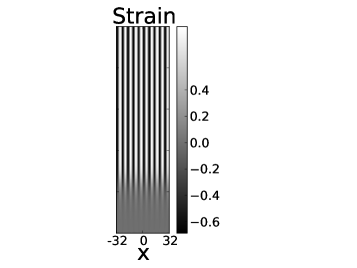
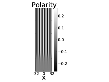
Figure 3: Stationary bifurcation. Numerical simulations of eqs. (9)-(11)-(23), were performed with XMDS2 Dennis2013 , with random initial conditions and periodic boundary conditions. The parameter values are: $a=1$, $K=1$, $w=1$, $\tau=\tau_{\mathrm{p}}=1$, $\lambda=1$, $\alpha_{\mathrm{a}}=2$, $\Gamma_{\mathrm{p}}=1$, $\nu=1$, leading to a threshold $l_{\mathrm{p}}^{c}=3$, see eq. (24). Space-time plots of the velocity, strain and polarity fields are shown immediately above threshold $l_{\mathrm{p}}=3.01$.

In the particular case of a velocity field equal to zero, the strain field is not transported (Eq. (10) does not apply). Upon substituting $\partial_{x}e$ from (9) into (11), we found that the polarity field evolves according to the damped Kuramoto-Sivashinsky equation

$$\partial_{t}p+\alpha_{\mathrm{a}}\;p\,\partial_{x}p=-\frac{1}{\tau_{\mathrm{p}}}\,p+\Gamma_{\mathrm{p}}\left(K-w\,l_{\mathrm{p}}\right)\,\partial_{x}^{2}p-\Gamma_{\mathrm{p}}\nu\,\partial^{4}_{x}p\,.$$ (22)

The polarity diffusion constant $D_{\mathrm{p}}=\frac{\Gamma_{\mathrm{p}}}{G}\,(KG-w^{2}-\beta_{\mathrm{a}}w)$ is positive in the absence of activity ($\beta_{\mathrm{a}}=0$) since $w^{2}\leq KG$. It may become negative in an active, polar material, leading to a stationary instability Yoshinaga2010 .

In the general case ($v\neq 0$), the strain field is transported according to $\dot{e}=\partial_{x}v$, and eq. (10) is replaced by

$$\partial_{t}e+v\,\partial_{x}e=\partial_{x}v\,.$$ (23)

The linear stability analysis of the homogeneous state $v=e=p=0$ unfolds as in section 3.1. For the system (9)-(11)-(23), the necessary condition for a stationary bifurcation is

$$wl_{\mathrm{p}}>K+2\sqrt{a\nu}$$ (24)

also written as

$$w\beta_{\mathrm{a}}>KG-w^{2}+2G\sqrt{a\nu}$$ (25)

In agreement with Yoshinaga2010 , the wavelength of the stationary pattern is that of the most unstable mode

$$\lambda_{0}=2\pi\sqrt{\frac{2\nu}{wl_{\mathrm{p}}-K}}=2\pi\sqrt{\frac{2\nu G}{w\beta_{\mathrm{a}}-(KG-w^{2})}}\,.$$ (26)

Depending on the experimental conditions, one may need to include external friction in the force balance equation, $\partial_{x}\sigma=\xi\,v$, with a positive friction coefficient $\xi$. In the case of a viscoelastic solid, one can easily show that this additional term leaves the threshold (24) unchanged.

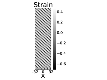
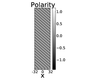
Figure 4: Propagating waves. Numerical simulations of eqs. (9)-(11)-(23) were performed with XMDS2 Dennis2013 , with periodic initial conditions, eqs. (18), with $k=0.5$ and $\varphi_{0}=0.5$, and periodic boundary conditions. Space-time plots of the velocity, strain and polarity fields are shown for the parameter values: $a=1$, $K=1$, $w=1$, $\tau=10$, $\lambda=1$, $\nu=1$, $\alpha_{\mathrm{a}}=2$, $\Gamma_{\mathrm{p}}=0.1$ ($\tau_{\mathrm{p}}=10$) and $l_{\mathrm{p}}=1.9$, above the threshold value $l_{\mathrm{p}}^{c}\simeq 1.63$ calculated from eq. (24).

Numerical simulations support the results of the linear stability analysis, see figure 3. Above threshold, stationary periodic patterns arise for the strain and polarity fields, whereas the velocity field quickly relaxes to zero (see eq. (23)), confirming the relevance of the analysis previously performed in the case of a zero velocity field Yoshinaga2010 . Using periodic initial conditions (18), numerical simlulations yield propagating waves for the velocity, strain and polarity fields at lower values of the polarity damping (figure 4).

References

- (1) F. Jülicher, K. Kruse, J. Prost, J.F. Joanny, Phys. Rep. 449, 3 (2007)
- (2) S. Ramaswamy, Annu. Rev. Cond. Matt. Phys. 1, 323 (2010)
- (3) M.C. Marchetti et al., Rev. Mod. Phys. 85, 1143 (2013)
- (4) D. Chen et al., Annu. Rev. Cond. Matter Phys. 1, 301 (2010)
- (5) K. Kruse et al., Phys. Rev. Lett. 92, 078101 (2004)
- (6) K. Kruse et al., Eur. Phys. J. E 16, 5 (2005)
- (7) S. Muhuri et al., Europhys. Lett. 78, 48002 (2007)
- (8) L. Giomi et al., Phys. Rev. Lett. 101, 198101 (2008)
- (9) S. Banerjee, T.B. Liverpool, M.C. Marchetti, Europhys. Lett. 96, 58004 (2011)
- (10) C.M. Edwards, U.S. Schwarz, Phys. Rev. Lett. 107, 128101 (2012)
- (11) N. Yoshinaga, P. Marcq, Phys. Biol. 9, 046004 (2012)
- (12) A.C. Callan-Jones, F. Jülicher, New. J. Phys. 13, 093027 (2011)
- (13) N. Yoshinaga, J.F. Joanny, J. Prost, P. Marcq, Phys. Rev. Lett. 105, 238103 (2010)
- (14) P. Manneville, The Kuramoto-Sivashinsky equation: a progress report, in Propagation in systems far from equilibrium, edited by J.E. Wesfreid et al. (1988), Vol. 40 of Springer Series in Synergetics, pp. 265–280
- (15) H. Brand, H. Pleiner, W. Renz, J. Phys. 51, 1065 (1990)
- (16) P. Chaikin, T. Lubensky, Principles of condensed matter physics (Cambridge University Press, 1995)
- (17) G.R. Dennis, J.J. Hope, M.T. Johnsson, Comp. Phys. Comm. 184, 201–208 (2013)
- (18) C. Misbah, A. Valance, Phys. Rev. E 49, 166 (1994)
- (19) P. Brunet, Phys. Rev. E 76, 017204 (2007)
- (20) R.K. Meyer, U. Aebi, J Cell Biol 110, 2013 (1990)
- (21) L.P. Cramer et al., J. Cell Biol. 136, 1287 (1997)
- (22) L.J. Peterson et al., Mol. Biol. Cell 15, 3497 (2004)
- (23) S. Ebrahim et al., Curr. Biol. 23, 731 (2013)
- (24) Y. Senju, H. Miyata, J. Biochem. 145, 137 (2009)
- (25) A. Kumar et al., Sci Rep 4, 3781 (2014)
- (26) U.S. Eggert, T.J. Mitchison, C.M. Field, Annu. Rev. Biochem. 75, 543 (2006)
- (27) Y. Asano et al., HFSP J. 3, 194 (2009)
- (28) O. Ilina, P. Friedl, J. Cell Sci. 122, 3203 (2009)
- (29) P. Rørth, EMBO Rep. 13, 984 (2012)
- (30) M.H. Köpf, L.M. Pismen, Soft Matter 9, 3727 (2012)
- (31) R. Farooqui, G. Fenteany, J Cell Sci 118, 51 (2005)
- (32) M. Reffay et al., Biophys. J. 100, 2566 (2011)
- (33) G.F. Weber, M.A. Bjerke, D.W. Desimone, Dev. Cell 22, 104–115 (2011)
- (34) R.A. Desai et al., J. Cell Sci. 122, 905 (2009)
- (35) J. Ranft et al., Proc. Natl. Acad. Sci. USA 107, 20863 (2010)
- (36) X. Serra-Picamal et al., Nat. Phys. 8, 628–634 (2012)
- (37) D. Bilder, S.L. Haigo, Dev. Cell 22, 12 (2012)
- (38) L.Q. Wan et al., Proc. Natl. Acad. Sci. USA 108, 12295 (2011)
- (39) C. Brangwynne et al., In Vitro Cell Dev Biol Anim 36, 563 (2000)
- (40) K. Tanner et al., Proc Natl Acad Sci USA 109, 1973 (2012)
- (41) J. Toner, Y. Tu, S. Ramaswamy, Ann. Phys. 318, 170 (2005)
- (42) A. Ahmadi et al., Phys. Rev. E 74, 061913 (2006)
- (43) M. Claessens, M. Bathe, E. Frey, A.R. Bausch, Nat. Mat. 5, 748 (2006)
- (44) D. Strehle et al., Eur. Biophys. J. 40, 93 (2011)
- (45) T. Thoresen, M. Lenz, M.L. Gardel, Biophys. J. 100, 2698 (2011)
- (46) S. Köhler, V. Schaller, A.R. Bausch, PLoS One 6, e23798 (2011)
- (47) L. Petitjean et al., Biophys. J. 98, 1790 (2010)
- (48) T.E. Angelini et al., Phys. Rev. Lett. 104, 168104 (2010)
- (49) M. Paniconi, K.R. Elder, Phys. Rev. E 56, 2713 (1997)