Direct numerical simulations of an inertial wave attractor in linear and nonlinear regimes

Abstract

In a uniformly rotating fluid, inertial waves propagate along rays that are inclined to the rotation axis by an angle that depends on the wave frequency. In closed domains, multiple reflections from the boundaries may cause inertial waves to focus on to particular structures known as wave attractors. These attractors are likely to appear in fluid containers with at least one boundary that is neither parallel nor normal to the rotation axis. A closely related process also applies to internal gravity waves in a stably stratified fluid. Such structures have previously been studied from a theoretical point of view, in laboratory experiments, in linear numerical calculations and in some recent numerical simulations. In the present paper, two-dimensional direct numerical simulations of an inertial wave attractor are presented. By varying the amplitude at which the system is forced periodically, we are able to describe the transition between the linear and nonlinear regimes as well as the characteristic properties of the two situations. In the linear regime, we first recover the results of the linear calculations and asymptotic theory of Ogilvie (2005) who considered a prototypical problem involving the focusing of linear internal waves into a narrow beam centred on a wave attractor in a steady state. The velocity profile of the beam and its scalings with the Ekman number, as well as the asymptotic value of the dissipation rate, are found to be in agreement with the linear theory. We also find that, as the beam builds up around the wave attractor, the power input by the applied force reaches its limiting value more rapidly than the dissipation rate, which saturates only when the beam has reached its final thickness. In the nonlinear regime, the beam is strongly affected and becomes unstable to a subharmonic instability. This instability transfers energy to secondary waves possessing shorter wavelengths and lower frequencies. The onset of the instability of a narrow inertial wave beam is investigated by means of a separate linear analysis and the results, such as the onset of the instability, are found to be consistent with the global simulations of the wave attractor. The excitation of such secondary waves described theoretically in this work has also been seen in recent laboratory experiments on internal gravity waves.

1 Introduction

Internal waves supported by buoyancy and Coriolis forces play an important role in the Earth’s ocean and atmosphere, and have been widely studied through theory and experiment. The simplest situations are those of pure internal gravity waves in a non-rotating, stably stratified fluid, and pure inertial waves in a rotating, unstratified fluid. There is a close analogy between these two cases.

Internal waves have properties quite different from acoustic or electromagnetic waves, being highly anisotropic and dispersive. In a frame of reference in which the mean flow vanishes, the wave frequency depends only on the direction, and not on the magnitude, of the wavevector. Special directions are defined by gravity or rotation. Energy propagates at the group velocity, which is perpendicular to the wavevector and inversely proportional to its magnitude. Internal waves are highly dispersive and do not steepen like acoustic waves, but instead break and dissipate when they exceed a critical amplitude and become locally unstable. Their frequencies are bounded and form a dense or continuous spectrum. In a closed domain, internal waves generally do not form normal modes with regular eigenfunctions, although the simplest cases are exceptions to this rule. Waves of a given frequency generally undergo focusing or defocusing when they reflect from boundaries; after multiple reflections in a generic container, rays are typically focused towards limit cycles known as wave attractors (Maas & Lam, 1995).

In the interiors of stars and giant planets, internal waves occupy the low-frequency part of the spectrum of oscillations, which can be excited by tidal forcing when the body has an orbiting companion (e.g Ogilvie & Lin, 2004). The question arises of how a rotating or stably stratified fluid responds to an oscillatory body force with a frequency that lies within the dense or continuous spectrum. For tidal applications, what is of particular interest is the rate at which energy is transferred to the fluid, ultimately to be dissipated. The relative amplitudes of astrophysical tides can vary enormously, depending on the relative mass and distance of the tide-raising body. It is therefore appropriate to investigate both linear and nonlinear regimes for internal tides.

Ogilvie (2005) considered a simple problem involving a two-dimensional fluid domain that supports internal waves, and calculated the steady-state linear response to a periodic body force with a frequency such that a wave attractor occurs. He obtained an analytical asymptotic solution in the limit that the dissipative effects of the fluid are small. The response is localized in a narrow beam centred on the attractor, and, for a body force of fixed amplitude, the dissipation rate (which is equal to the power input) is asymptotically independent of both the magnitude and the details of the dissipative process. This situation occurs because the attractor acts as a ‘black hole’ that absorbs a certain energy flux from the waves being focused into it. This result contrasts strongly with a situation in which the internal waves form classical normal modes, as in the case of inertial waves in a rectangular container whose walls are parallel and perpendicular to the rotation axis. In such a situation, the dissipation rate is simply proportional to the viscosity, and therefore astrophysically unimportant, unless the forcing frequency matches the natural frequency of a normal mode and a resonance occurs.

Internal wave attractors have been seen in experiments (Maas et al., 1997; Maas, 2001; Manders & Maas, 2003; Lam & Maas, 2008; Hazewinkel et al., 2008, 2011a, 2011b; Scolan et al., 2013), linear calculations (Rieutord & Valdettaro, 1997; Dintrans et al., 1999; Rieutord et al., 2001; Ogilvie, 2005; Maas & Harlander, 2007; Ogilvie, 2009; Rieutord & Valdettaro, 2010; Echeverri et al., 2011; Bajars et al., 2013; Baruteau & Rieutord, 2013) and numerical simulations (Grisouard et al., 2008). The wave attractor is a linear phenomenon and one may naturally ask how it is modified by nonlinearity. Previous experiments (Maas, 2001) have shown some evidence for cumulative nonlinear effects that build up over a large number of wave periods: the fluid becomes increasingly mixed, and momentum deposition leads to the generation of a mean flow. Until recently, no evidence had been found for stronger nonlinear phenomena such as wave breaking, instability or turbulence. However, Scolan et al. (2013) have recently reported experiments on internal gravity waves in which waves focused towards an attractor become unstable and divert energy to smaller scales. They describe this process as a parametric subharmonic instability similar to that known for plane internal waves.

The purpose of this work is to study a simple system of periodically forced inertial waves in a closed domain by means of fully nonlinear direct numerical simulations. We aim first to recover the results of Ogilvie (2005) for the steady-state response of a wave attractor in a linear regime, and to understand how this steady state is achieved. Moving into the nonlinear regime, we aim to locate the onset of instability and to see how the attractor operates, if at all, in the presence of instability. We will compare our results with the experimental findings of Scolan et al. (2013). Of particular interest is the energy budget of the system and the question of how the dissipation rate (and thence the tidal torque, in astrophysical applications) is affected by nonlinearity.

2 Model and governing equations

2.1 Description of the model

In this section, we present the model system that we use to study the forcing of inertial waves in a closed two-dimensional (2D) domain. A similar model was used by Ogilvie (2005) for analytical and numerical calculations of forced linear internal waves. Perhaps the simplest domain exhibiting a wave attractor is a square that is tilted with respect to the rotation axis. We therefore adopt Cartesian coordinates $(x,y,z)$ in a rotating frame of reference and solve the incompressible Navier–Stokes equation in a square domain $-L/2<\{x,z\}<L/2$ with the angular velocity vector $\boldsymbol{\Omega}$ in the $xz$ plane and inclined by an angle $\theta$ with respect to the $z$ axis (Fig. 1). The problem is invariant and unbounded in the $y$ direction and the fluid velocity $\boldsymbol{v}$ has three components.

For wave frequencies smaller than twice the rotation frequency ($|\omega|<2\Omega$), the spatial structure of inviscid linear waves in the $xz$ plane is described by a hyperbolic equation (the Poincaré equation), whose characteristic rays are straight lines inclined at angles $\pm\arcsin(\omega/2\Omega)$ with respect to the rotation axis. Indeed, the dispersion relation relates the frequency and the direction of propagation (which is perpendicular to the wavevector $\boldsymbol{k}$) through $\omega=\pm 2\boldsymbol{\hat{k}}\cdot\boldsymbol{\Omega}$, where $\boldsymbol{\hat{k}}=\boldsymbol{k}/|\boldsymbol{k}|$.

The rotation axis in our model is inclined with respect to the boundaries so that, allowing for multiple reflections from the walls, the rays tend to focus on to localized singular structures known as wave attractors (Maas & Lam, 1995). (In the case of aligned rotation, i.e. $\theta=0$, the rays instead propagate ergodically through the domain, except for special frequencies for which they propagate periodically.) A body force is applied to the system at a particular temporal frequency (less than $2\Omega$) to mimic the effect of tidal forcing. In order to excite waves in an incompressible fluid in a closed domain, a non-potential force must be applied, and the origin of this vortical effective force in a tidal problem with free boundaries is explained in Ogilvie (2005). Contrary to the turbulent wave excitation in a convective environment, for example, tidal forcing is strictly periodic (or nearly so) and thus can be easily imposed in our equation of motion.

The governing equations for a homogeneous viscous incompressible fluid in a rotating frame are then

$$\frac{\partial\boldsymbol{v}}{\partial t}+(\boldsymbol{v}\cdot\boldsymbol{\nabla})\boldsymbol{v}+2\boldsymbol{\Omega}\times\boldsymbol{v}=-\boldsymbol{\nabla}P+\nu\,\nabla^{2}\boldsymbol{v}+\boldsymbol{a},$$ (1)

$$\nabla\cdot\boldsymbol{v}=0,$$ (2)

where $P$ is a modified pressure that incorporates the gravitational and centrifugal potentials, and $\boldsymbol{a}$ is the body force per unit mass. As explained above, only the rotational part of $\boldsymbol{a}$ drives the fluid motion in a closed container. We adopt a simple expression for $\boldsymbol{a}$, linear in the Cartesian coordinates, such that

$$\boldsymbol{\nabla}\times\boldsymbol{a}=F_{0}\cos(\omega_{0}t)\,\boldsymbol{e}_{y}$$ (3)

is uniform, as in the numerical example studied by Ogilvie (2005).

We use $1/2\Omega$ as the unit of time and $L$, the size of the domain in which the fluid is contained, as the unit of length. The rotation vector is inclined as shown in Fig. 1, leading to the following expression for $\Omega$:

$$2\boldsymbol{\Omega}=(\cos\theta\,\boldsymbol{e}_{z}-\sin\theta\,\boldsymbol{e}_{x})$$ (4)

For all the simulations presented here, we choose $\omega_{0}/2\Omega=\sin(\pi/4)=\sqrt{2}/2$ so the angle of wave propagation with respect to the rotation axis is $\pi/4$. We also choose the inclination angle $\theta$ such that $\tan\theta=1/3$, which results in a theoretically square wave attractor inside the square domain, reflecting from each wall one-third of the way along its length $L$ (Fig. 1).

The remaining dimensionless parameters to be chosen are the Ekman number $Ek=\nu/2\Omega L^{2}$ and the dimensionless forcing amplitude $F_{0}/(2\Omega)^{2}$. We work with dimensionless variables, choosing units such that $L=2\Omega=1$, so that $Ek=\nu$.

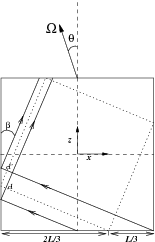
Figure 1: Sketch of the fluid domain and wave attractor. The dotted line represents the theoretical spatial structure of the inertial wave attractor in this situation. The focusing of one beam of width $d$ is shown for one reflection at the left boundary. The resulting beam has width $d^{\prime}=d/2$.

A sketch of the geometry is shown in Fig. 1. The square domain is represented together with the inclined rotation vector. An illustrative example of one reflection on the left boundary of an inviscid inertial wave beam is shown, where the focusing effect is quite clear. It is easy to show that in this situation, the focusing factor for one reflection is 2, i.e. $d^{\prime}=d/2$ with the notations chosen here.

2.2 Numerical implementation

To solve our problem numerically, we use SNOOPY, a 3D spectral code solving the equations of incompressible or Boussinesq (magneto)hydrodynamics using a Fourier representation (Lesur & Longaretti, 2005, 2007; Lesur & Ogilvie, 2010). We here compute the evolution of the velocity field in 2D (in the $xz$ plane) by putting only one point in the $y$ direction. The spatial computational domain is $-L_{\mathrm{c}}/2<\{x,z\}<L_{\mathrm{c}}/2$ and the typical resolution we use is $256\times 256$. To impose rigid, no-slip boundary conditions at the four edges of the fluid domain $-L/2<\{x,z\}<L/2$, we apply a mask in physical space on the velocity field so that all three components of the velocity are forced to vanish in the part of the domain outside the fluid, which is such that $L/L_{\mathrm{c}}=0.8$. By applying this mask in the physical space after each sub-timestep of the third-order Runge–Kutta method, we inevitably have a loss of energy in the neighbourhood of the boundaries. Both increasing the spatial resolution (to resolve the boundary layers) and decreasing the time step (to decrease the error linked to the mask) lead to a convergence towards zero of the loss of energy. In the cases shown here, a resolution of $256$ collocation points per dimension was found to be enough to ensure energy conservation to an accuracy of a few percent.

The initial condition we use is zero-velocity but, since a body force is applied to the system, a velocity field rapidly sets in, consisting of inertial waves whose temporal evolution we wish to follow in various situations. We start with the linear cases to which analytical results can be compared and then increase the amplitude of the force to trigger nonlinearities in the system.

Figure 2: Snapshots of $v_{z}$ inside the domain at times $0$, $T/4$, $T/2$ and $3T/4$, where $T=2\pi/\omega_{0}$ is the wave period. The instant labelled $t=0$ already corresponds here to about 45 wave periods, at a time when the beam centred on the attractor has reached its final structure.

3 The linear regime

3.1 General properties of the steady-state response and comparison with theory

An illustrative example is shown in Fig. 2 of a direct numerical simulation of an inertial wave attractor quickly developing in our computational domain. The forcing amplitude is chosen here to be small enough ($F_{0}=7.5\times 10^{-4}$) so that the nonlinear terms do not play a significant role. During a relatively short transient phase (a few tens of wave periods), the structure of the wave attractor starts to appear, forming a square shape inside our domain. The figure shows the oscillatory flow that is established after this transient phase. The inertial wave beam, an oscillating shear layer formed around the attracting structure, is clearly visible, the excitation being optimal in this case. We also see in this figure the transverse character of the inertial waves, with the phase propagating perpendicular to the beam.

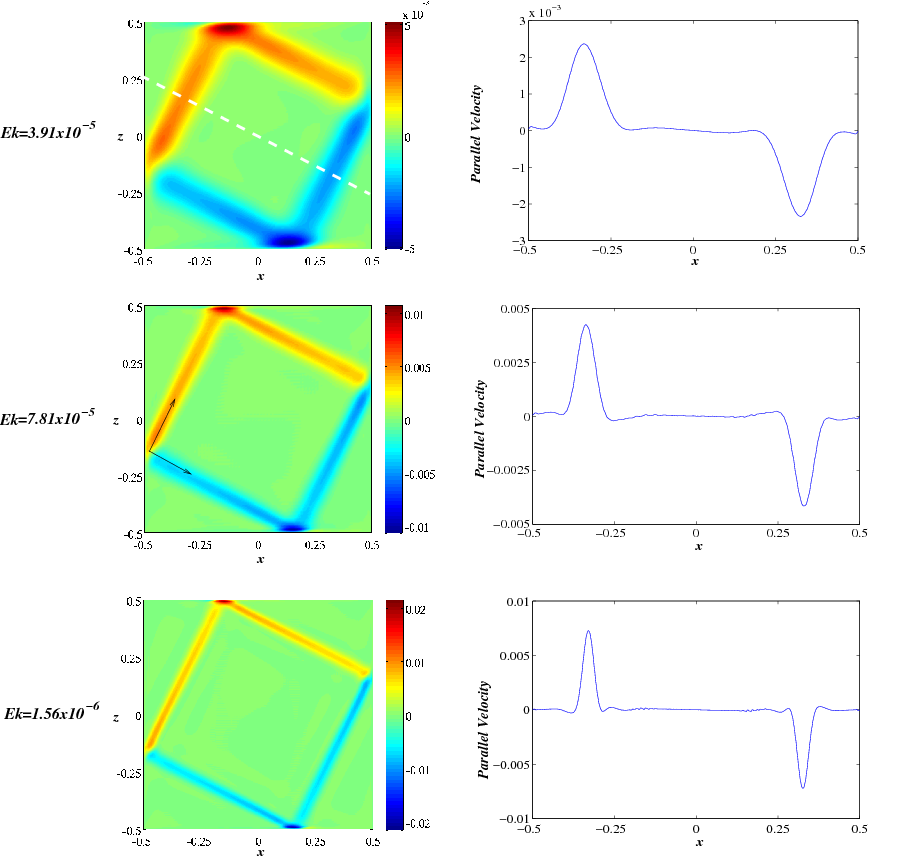
Figure 3: Snapshot of the velocity component parallel to the attractor after the structure has settled (left panels), and a cut of the same velocity (right panels) through the attractor, along the white dashed line represented in the top left panel, for 3 different values of the Ekman number.

The first analysis we make is to test in a simple way the predicted scaling of the thickness of the beam with the viscosity (Ogilvie, 2005), namely that the width scales with $Ek^{1/3}$ where $Ek$ is the Ekman number. We thus study simulations with various Ekman numbers at a fixed forcing amplitude $F_{0}=7.5\times 10^{-4}$ and measure the width of the beam in each case. Illustrative results are shown in Fig. 3, where we present for three different values of the Ekman number, a snapshot of the component of the velocity parallel to the beam. The spatial structure of the attractor then clearly appears. We add to these snapshots a cut through the attractor of this parallel velocity for each case. The thickness of the beam is measured in those various cases (we spanned $Ek$ values from $7.81\times 10^{-5}$ to $1.56\times 10^{-6}$) and we find a good agreement with the theoretical scaling of $Ek^{1/3}$.

We now proceed to a detailed comparison of the simulations with the theoretical predictions, looking at the velocity profiles along various cuts through the attractor. We examine both the component parallel to the attractor, $v_{\|}$, and the component perpendicular to the $xz$ plane, $v_{y}$. The velocity component perpendicular to the attractor and within the $xz$ plane is much smaller.

In each segment of the attractor, the solution takes the form of an internal wave beam that spreads self-similarly along its length because of viscosity (cf. Moore & Saffman, 1969). The scaling properties of the beam are easily understood if we consider a narrow beam emitted from a theoretical point source. Since the group velocity of an internal wave is proportional to its wavelength and directed perpendicular to the wavevector, the wave propagates along the beam at a speed proportional to the width of the beam. As the width increases as $t^{1/2}$ because of viscous diffusion, so the distance parallel to the beam increases as $t^{3/2}$. Therefore the width and the group velocity increase with the distance to the power $1/3$.

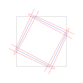
Figure 4: Representation of the boundary of the fluid domain (black), the wave attractor (blue) and the pattern of self-similarly spreading inertial-wave beams in a steady state (red), with virtual sources outside the fluid domain. The width of the beam doubles by viscous diffusion along each segment, but is halved at each reflection.

In a steady state, the viscous spreading of the beam is balanced globally by the focusing of the beam at its reflection points. In our case the width of the beam is halved on each reflection. It follows that each segment of the beam has a virtual source that is located outside the fluid domain at a parallel distance that is $1/7$ of the length of one side of the attractor. This ensures that the width of the beam is doubled between each reflection. The pattern of beams and virtual sources is indicated in Fig. 4.

Ogilvie (2005) makes detailed predictions for the streamfunction of the flow within the plane in the steady-state response in the asymptotic limit of small Ekman number, where the beam is narrow. The ‘inner solution’ found in the neighbourhood of the attractor contains, in principle, an infinite series of modes with different structures parallel and perpendicular to the attractor. Much of the complexity of the analysis comes from having to determine the amplitudes of the higher modes, $n\geq 1$, which have an oscillatory structure in the direction parallel to the beam. The amplitude $a_{0}$ of the ‘fundamental’ $n=0$ mode is much more easily determined. Furthermore, it is found that the $n=0$ mode dominates the response in the case we consider here, where the body force is very smooth and its curl is independent of position. We therefore recall only this component of the asymptotic inner solution and compare it with the results of our simulations.

Translating the results of Ogilvie (2005) into the context and notations of the present paper, we expect that

$$v_{\|}=\mathrm{Re}[U(\tau,\mu)\exp(-i\omega_{0}t)],$$ (5)

$$v_{y}=\mathrm{Re}[iU(\tau,\mu)\exp(-i\omega_{0}t)],$$ (6)

where $\omega_{0}$ is the forcing frequency (which is also the frequency of the primary wave), and $U$ is a complex velocity profile given by

$$U(\tau,\mu)=\left(\frac{\omega_{0}}{\nu\mu}\right)^{1/3}a_{0}\,\,\chi_{0}^{\prime}(\tau).$$ (7)

Here $\mu$ is the distance along the beam from the virtual source and $\tau$ the transverse distance $\tilde{\tau}$ scaled by $\mu^{-1/3}$ and multiplied by $(\omega_{0}/\nu)^{1/3}$ to keep the dimension of a distance. The velocity components are scaled with $\mu^{-1/3}$ to take into account the increase of the group velocity during propagation along the wave beam. If we consider the leftmost corner of the attractor, the virtual source being located at $x_{\mathrm{s}},z_{\mathrm{s}}$, the expressions for $\mu$ and $\tau$ are

$$\mu=(x-x_{\mathrm{s}})\sin\beta+(z-z_{\mathrm{s}})\cos\beta,$$ (8)

$$\tilde{\tau}=(x-x_{\mathrm{s}})\cos\beta-(z-z_{\mathrm{s}})\sin\beta,$$ (9)

$$\tau=\left(\frac{\omega_{0}}{\nu\mu}\right)^{1/3}\tilde{\tau},$$ (10)

where $\beta$ is the angle between the vertical boundary and the beam, shown in Fig. 1.

The amplitude coefficient of the ‘fundamental’ $n=0$ mode as described above is

$$a_{0}=\frac{\delta}{\ln\alpha},$$ (11)

where $\delta$ and $\alpha$ are respectively the forcing and focusing constants. The focusing constant $\alpha$ represents the focusing experienced by a wave beam in one full circuit around the container. In our case, each reflection at the boundary focuses our beam by a factor $2$. In one full loop, the beam undergoes four reflections and the focusing factor is thus $\alpha=2^{4}=16$.

The factor $\delta$ is related to the change in the streamfunction around each circuit of the wave attractor, due to the body force. In our problem it is defined in the following way:

$$\delta=\frac{i}{2\omega_{0}}\int(\boldsymbol{\nabla}\times\boldsymbol{a})_{y}\,\,\mathrm{d}A,$$ (12)

where the integral is computed over the area enclosed by the attractor, and a time-dependence of $\exp(-i\omega_{0}t)$ is understood for the forcing. [This expression differs by a factor of $-2\omega_{0}$ from the one in Ogilvie (2005) because the problem was defined slightly differently in that paper.] In our case, it is thus equal to

$$\delta=\frac{i}{2\omega_{0}}\,\,F_{0}\,\,\frac{5L^{2}}{9}.$$ (13)

Figure 5: Real and imaginary parts (solid and dashed lines) of the dimensionless velocity profile of the beam.

Finally $\chi_{0}(\tau)$ is the transverse profile of the streamfunction, which satisfies an ordinary differential equation whose solutions are obtained by the Laplace transform of Moore & Saffman (1969). The first derivative $\chi_{0}^{\prime}$ which appears in the expression for the parallel velocity (and also for the $y$-velocity, which is related to it through the Coriolis force) has the following integral representation:

$$\chi_{0}^{\prime}(\tau)=i\int_{0}^{\infty}\exp(-ip\tau-p^{3})\,\mathrm{d}p=ig(-\tau).$$ (14)

Note that the complex function $g(\tau)$ is composed purely of positive wavenumbers; its real and imaginary parts are plotted in Figure 5, and its maximum modulus is $\max|g|=g(0)=\Gamma({\textstyle\frac{4}{3}})\approx 0.8930$.

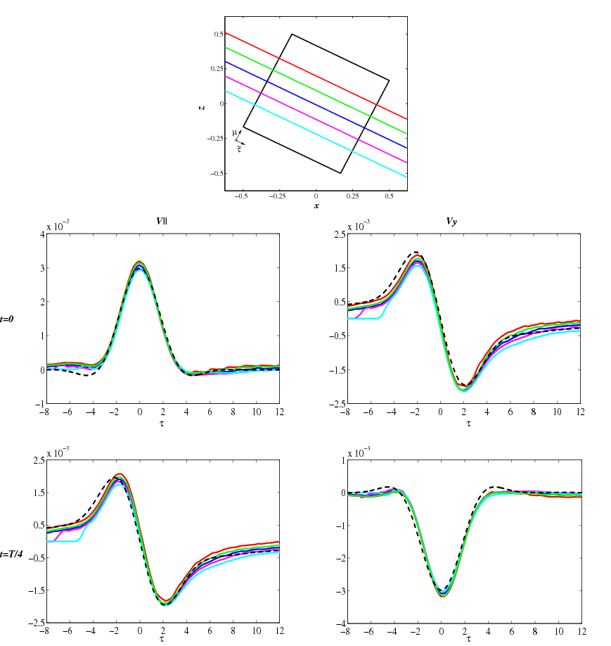
Figure 6: Top panel: sketch of the attractor inside the container with a representation of the various cuts made through the attractor, for which the profiles of the parallel and the $y$-velocities are shown. The red dot at the bottom left of the sketch marks the position of the virtual source, i.e. the origin of the coordinate system $(\tilde{\tau},\mu)$. Four other panels: cuts of the velocities parallel and perpendicular to the beam, as a function of the scaled transverse distance $\tau$ (shown on the top panel). The point $\tau=0$ indicates the centre of the wave beam. The cuts are represented at the same times as the two upper panels of Fig. 2. The colored lines show the results of the simulations and the dotted black line the theoretical prediction.

Figure 6 shows cuts at different distances from the virtual source along the beam of the parallel and perpendicular velocities, rescaled by $\mu^{1/3}$ to account for viscous spreading. The cuts are shown as functions of the scaled transverse distance $\tau$, $\tau=0$ corresponding to the centre of the beam. The case shown here is at $Ek=7.81\times 10^{-6}$. The theoretical velocities given by expressions (5) and (6) and also rescaled by $\mu^{1/3}$ are superimposed on those curves. This figure shows a fairly good agreement between the theoretical profile and the simulated attractor at various temporal phases in the steady-state. We indeed find that both the amplitude of the velocities and the width of the beam scale with the distance to the virtual source to the power $1/3$. In agreement with what was shown in Fig. 2, the parallel velocity is positive and maximum at temporal phase $t=0$ and changes sign at $\tau=0$ at temporal phase $t=T/4$. It is the opposite for the $y$-velocity, as also expected from the theory. We note that the theoretical profiles are symmetric or antisymmetric with respect to the centre of the beam at these temporal phases. This is verified in the simulations but this is more easily seen for cuts made far from the virtual source (green and red curves) where the left boundary of the domain does not affect the velocity profiles.

3.2 Building an inertial wave attractor

An interesting aspect of the problem that is revealed through direct numerical simulations of the wave attractor is the transient evolution from the initial state with zero velocity to the formation of the final steady-state oscillatory solution described in Ogilvie (2005). Fig. 7 shows the temporal evolution of the $z$-component of the velocity inside the attractor from the beginning of the simulation, for two different values of the Ekman number, namely $Ek=7.81\times 10^{-5}$ and $Ek=7.81\times 10^{-6}$. The transient evolution is different in these two cases. Since the waves are focused into a spatial structure of smaller transverse extent in the case where the viscosity is smaller, and the group velocity of the waves diminishes in this process, it takes longer to establish the steady state. To be more precise, in the case where $Ek=7.81\times 10^{-5}$, the steady state is reached in about 5 wave periods, while, in the $Ek=7.81\times 10^{-6}$ case, we need to wait about twice as long before the simulation settles. This is consistent with the scaling of the thickness of the attractor with $Ek$. Since the width of the beam scales with $Ek^{1/3}$, and the group velocity is proportional to the wavelength, the time it takes to reach the steady state also scales with $Ek^{1/3}$. Consequently, if a steady state is reached in about 5 wave periods in the $Ek=7.81\times 10^{-5}$ case, it will be reached in about $5\times 10^{1/3}\approx 10.5$ wave-periods in the $Ek=7.81\times 10^{-6}$ case, which is consistent with our numerical results.

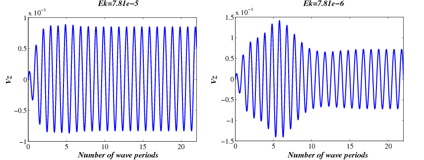
Figure 7: Temporal evolution of the vertical velocity $v_{z}$ at a point located inside the attractor, from the beginning of the simulation, in cases where $Ek=7.81\times 10^{-5}$ (left panel) and $Ek=7.81\times 10^{-6}$ (right panel).

If we now focus on the energy balance in the system, we can compare the energy input by the forcing term in the Navier–Stokes equation and the energy dissipation due to the viscous term. For the total kinetic energy to be conserved, these two terms should exactly balance each other in the steady state, when averaged over one oscillation cycle. More precisely, we should have in our case where $\nu$ is constant:

$$\int_{\cal{D}}\,\,\,\frac{\partial}{\partial t}\left(\frac{v^{2}}{2}\right)\,\mathrm{d}A=\int_{\cal{D}}\,\,\,\boldsymbol{a}\cdot\boldsymbol{v}\,\mathrm{d}A+\nu\int_{\cal{D}}\,\,\,\boldsymbol{v}\cdot\nabla^{2}\boldsymbol{v}\,\mathrm{d}A,$$ (15)

where $\cal{D}$ designates the fluid domain. Equivalently,

$$\frac{\mathrm{d}}{\mathrm{d}t}\int_{\cal{D}}\,\,\,\frac{v^{2}}{2}\,\mathrm{d}A=\int_{\cal{D}}\,\,\,\boldsymbol{a}\cdot\boldsymbol{v}\,\mathrm{d}A-\nu\int_{\cal{D}}\,\,\,|\boldsymbol{\nabla}\times\boldsymbol{v}|^{2}\,\mathrm{d}A,$$ (16)

which shows that the rate of change of the total kinetic energy is the difference of the power input by the body force and the viscous dissipation rate.

We are here interested in the transient evolution and more precisely in the time it takes for the power input to reach its steady state compared to the time it takes for the dissipation rate to settle. Moreover, in the steady state, the asymptotic value (when $Ek$ tends to $0$) of the dissipation rate derived in Ogilvie (2005) can be compared to our numerical results. In particular, we wish to investigate the possible independence of the dissipation rate with viscosity when $Ek$ tends to $0$.

Figure 8: Energy input versus dissipation: temporal evolution from the beginning of the simulation, focus on the transient phase.

We first focus on the simulation at $Ek=7.81\times 10^{-6}$ with a forcing amplitude of $F_{0}=7.5\times 10^{-4}$ and compute the power input by the force as well as the viscous dissipation rate. Figure 8 shows these quantities. The black line represents the power input, temporally averaged over a wave period. The red curve represents the evolution of the dissipation rate from the initial state until it reaches a well-established steady state. It is quite clear from this figure that the time-scale for saturation of the power input is much shorter than that of the viscous dissipation. The typical time it takes for the power to reach a steady state is about 4–5 wave periods while the saturation time for the dissipation rate is about 14 periods. The significance of this result is that, while the waves are still in the process of being focused towards the attractor and approaching the scale on which they can be dissipated, the energy flux into the attractor has already reached its asymptotic value. Only later will the energy flux be matched by viscous dissipation in a steady state. At that time, a final value of the dissipation rate will be reached, which, for a fixed value of the forcing amplitude $F_{0}$, should be asymptotically independent of the value of the Ekman number, as shown in Ogilvie (2005).

We note that in our simulation, a discrepancy exists in the saturated regime between the mean power exerted by the force and the dissipation rate. As stated in the first section, this is due to the way the rigid walls are applied in the SNOOPY code, which uses decomposition on Fourier modes and thus usually deals with periodic boundary conditions. The application of a mask on the velocity adds an error of the order of $\Delta t$ in the numerical scheme and thus causes the system to lose part of its energy at the boundaries. Decreasing the time step and increasing the resolution to solve for the viscous boundary layers appearing close to the walls both help to reduce this loss of energy. Various convergence tests were run to have a clear control on the effects of the mask and it was found that the typical time it takes to reach a steady state is not strongly affected; only the final value of the dissipation rate is sensitive to the spatial resolution and time step. In the best cases we have, the energy is conserved at the level of a few percent.

The value of the viscosity was then varied to investigate the transient phase for different Ekman numbers. The results are shown in Fig. 9, where only the dissipation rate is represented. It is clear from this plot that the time it takes for the dissipation rate to saturate depends on the viscosity. As stated before, we find that this typical time scales with $Ek^{-1/3}$, a similar scaling to what is found for the width of the final wave beam. However, the long-term dissipation rate seems to approach a limiting value, asymptotically independent of the Ekman number for $Ek\ll 1$, as shown by Ogilvie (2005). To have a better comparison to his analytical results, we compute the theoretical value of the asymptotic dissipation rate in the present system. For a smooth forcing function (which we have here), it is shown that the dominant contribution to the dissipation rate is made by the coefficient $a_{0}$ whose expression was given above (see Eq. 11).

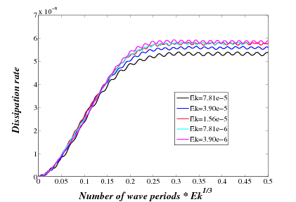
Figure 9: Evolution of the average dissipation rate in the domain for various values of the viscosity, as a function of time scaled by $Ek^{1/3}$.

The value of the asymptotic dissipation rate is then obtained by the expression derived by Ogilvie (2005):

$$D\approx 2\omega_{0}\,\frac{\pi}{2}\,\,\ln\alpha\,\,|a_{0}|^{2}=\omega_{0}\frac{\pi|\delta|^{2}}{\ln\alpha}.$$ (17)

The factor $2\omega_{0}$ appears because of the conversion of notation between the present problem and the one studied by Ogilvie (2005). In our case here where $F_{0}=7.5\times 10^{-4}$, we find an expected asymptotic value of $6.955\times 10^{-8}$. In figure 9, the dissipation rate seems to saturate at a lower value but this is again due to the fact that a small discrepancy exists between the work done by the force and the dissipation rate. If energy conservation was perfect in our domain, the dissipation rate would saturate at the same value as the rate of working. Since the latter is less affected by the application of the mask, we computed the asymptotic value reached by the power input and we obtained $D=6.65\times 10^{-8}$ for $Ek=7.81\times 10^{-6}$ and $D=6.74\times 10^{-8}$ for $Ek=3.9\times 10^{-6}$, thus very close to the asymptotic value found analytically.

4 Nonlinear cases

We now investigate the effect of increasing the amplitude of the body force. The idea is that we will reach a level where the nonlinear term will start to play a role and affect the spatial and temporal structure of the attractor.

4.1 Linear analysis of the instability of an inertial wave beam

In order to anticipate the behaviour of the nonlinear cases and in particular the characteristics of the possible instabilities which could occur, we carry out a local analysis of a narrow inertial wave beam, such as occurs in the presence of a wave attractor. We consider a simpler problem here, working in an $xy$ plane such that the primary motion is a narrow inertial wave beam aligned with the $x$-axis (i.e. a different coordinate system from the global attractor but without loss of generality or consequences on the characteristics of the instability). The equations considered are the same as Eqs. 1 and 2. We examine the dynamics on scales comparable to the width of the beam, and therefore assume periodic boundary conditions in $x$, neglecting the viscous spreading of the beam along its length. Consistent with this approximation, we also neglect the smaller $y$ component of the velocity. The beam can then be described as

$${\bf{u}}={\bf{u}}_{\mathrm{b}}=u(y,t)\,{\bf{e}}_{x}+w(y,t)\,{\bf{e}}_{z}=\mathrm{Re}\{[U(y)\,{\bf{e}}_{x}+W(y)\,{\bf{e}}_{z}]\,\mathrm{e}^{-\mathrm{i}\omega_{\mathrm{b}}t}\},$$ (18)

$$p=\mathrm{Re}[P(y)\,\mathrm{e}^{-\mathrm{i}\omega_{\mathrm{b}}t}],$$ (19)

where $U(y)$, $W(y)$ and $P(y)$ are complex amplitudes and $\omega_{\mathrm{b}}$ is the beam frequency. The basic equations are satisfied if

$$-\mathrm{i}\omega_{\mathrm{b}}U+2\Omega_{y}W=0,$$ (20)

$$-2\Omega_{x}W=-\partial_{y}P,$$ (21)

$$-\mathrm{i}\omega_{\mathrm{b}}W-2\Omega_{y}U=0,$$ (22)

which implies $\omega_{\mathrm{b}}=\pm 2\Omega_{y}$, with $W=\pm\mathrm{i}U$ respectively. Nonlinear effects are absent because ${\bf{u}}_{\mathrm{b}}\cdot{\nabla}{\bf{u}}_{\mathrm{b}}=\mathbf{0}$. To sustain the beam against viscous dissipation, a body force $a=-\nu\nabla^{2}{\bf{u}}_{\mathrm{b}}$ must be applied. (In the context of the wave attractor, the viscous force leads instead to a gradual spreading of the beam along its length, which is compensated by focusing at the points of reflection. In the local model, we could allow the beam to decay freely, but applying a body force has the advantage of maintaining a constant amplitude in the absence of instability.)

To understand the choice of signs, let us consider the dispersion relation for 2D inviscid inertial waves,

$$\omega^{2}=\frac{4(\Omega_{x}k_{x}+\Omega_{y}k_{y})^{2}}{k_{x}^{2}+k_{y}^{2}},$$ (23)

which implies a group velocity ${\bf{v}}_{\mathrm{g}}$ given by

$$2\omega v_{\mathrm{g}x}=\frac{8\Omega_{x}(\Omega_{x}k_{x}+\Omega_{y}k_{y})}{k_{x}^{2}+k_{y}^{2}}-\frac{8k_{x}(\Omega_{x}k_{x}+\Omega_{y}k_{y})^{2}}{(k_{x}^{2}+k_{y}^{2})^{2}},$$ (24)

and similarly for $v_{\mathrm{g}y}$. In the limit $k_{x}\to 0$ relevant for the beam, we have

$$v_{\mathrm{g}x}\to\frac{4\Omega_{x}\Omega_{y}}{\omega k_{y}}.$$ (25)

If we set up the problem such that $\Omega_{x}>0$ and $\Omega_{y}>0$, and choose the solution with the positive signs, then $\omega_{\mathrm{b}}>0$. If the beam is composed of positive wavenumbers $k_{y}>0$, then $v_{\mathrm{g}x}$ will be positive and the beam will propagate in the $+x$ direction.

As stated in Section 3.1, we assume that the relevant velocity profile of the beam is given by the dominant $n=0$ mode (Ogilvie, 2005; Moore & Saffman, 1969; Thomas & Stevenson, 1972) so that

$$U(y)=U_{0}g(\tau)=U_{0}\int_{0}^{\infty}\exp(-k^{3}+\mathrm{i}k\tau)\,\mathrm{d}k,$$ (26)

where $U_{0}>0$ is the beam amplitude and $\tau=y/L_{\mathrm{b}}$ is a dimensionless transverse $y$ coordinate, scaled by a characteristic beam width $L_{\mathrm{b}}$.

In terms of the streamfunction $\psi$ and the relative vorticity $\omega_{z}$ of the flow in the $xy$ plane, we have

$$u_{x}=\partial_{y}\psi,\qquad u_{y}=-\partial_{x}\psi,\qquad\omega_{z}=\partial_{x}u_{y}-\partial_{y}u_{x}=-\nabla^{2}\psi,$$ (27)

and the basic equations become

$$(\partial_{t}+{\bf{u}}\cdot{\nabla})\omega_{z}-2{\bf{\Omega}}\cdot{\nabla}u_{z}=\nu\nabla^{2}\omega_{z}+\partial_{x}a_{y}-\partial_{y}a_{x},$$ (28)

$$(\partial_{t}+{\bf{u}}\cdot{\nabla})u_{z}-2{\bf{\Omega}}\cdot{\nabla}\psi=\nu\nabla^{2}u_{z}+a_{z}.$$ (29)

We linearize these equations about the beam solution, assuming perturbations $\propto\mathrm{e}^{\mathrm{i}k_{x}x}$, to obtain

$$(\partial_{t}+\mathrm{i}k_{x}u)\omega_{z}^{\prime}+\mathrm{i}k_{x}\psi^{\prime}\partial_{y}^{2}u-2(\Omega_{x}\mathrm{i}k_{x}+\Omega_{y}\partial_{y})u_{z}^{\prime}=\nu(-k_{x}^{2}+\partial_{y}^{2})\omega_{z}^{\prime},$$ (30)

$$(\partial_{t}+\mathrm{i}k_{x}u)u_{z}^{\prime}-\mathrm{i}k_{x}\psi^{\prime}\partial_{y}w-2(\Omega_{x}\mathrm{i}k_{x}+\Omega_{y}\partial_{y})\psi^{\prime}=\nu(-k_{x}^{2}+\partial_{y}^{2})u_{z}^{\prime},$$ (31)

with

$$\omega_{z}^{\prime}=(k_{x}^{2}-\partial_{y}^{2})\psi^{\prime},$$ (32)

where the primes denote the perturbed quantities. We treat the $y$ direction numerically by taking a Fourier transform and discretizing the wavenumber $k_{y}$ on a regular grid, which leads to a large system of coupled linear ordinary differential equations (ODEs) in $t$. In practice this is equivalent to solving the problem in a finite domain of width $L_{y}$ with periodic boundary conditions. Since the beam is then not isolated but is effectively surrounded by periodic copies, we aim to make $L_{y}\gg L_{\mathrm{b}}$ and to seek localized instabilities that do not rely on the periodic repetition of the beam.

Since $u$ and $w$ are periodic in $t$, this is a Floquet problem. We integrate the system of ODEs forwards in time over one beam period $T_{\mathrm{b}}=2\pi/\omega_{\mathrm{b}}$ starting from many different initial conditions that span the space of initial data, i.e. by making as many computations as the number of ODEs. This generates the monodromy matrix that determines the evolution of an arbitrary initial condition over one beam period. We calculate the eigenvalues $\lambda$ of the monodromy matrix, which are the characteristic multipliers of the Floquet analysis, and we deduce the complex growth rates $s$ from the relation $\lambda=\exp(sT_{\mathrm{b}})$. The beam is unstable if $\mathrm{Re}(s)>0$ for any mode. The frequency of the instability is given by $\mathrm{Im}(s)$, but this is defined only modulo $\omega_{\mathrm{b}}$.

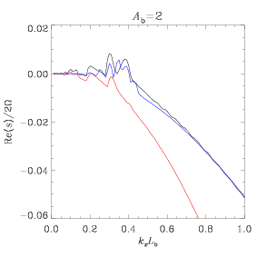
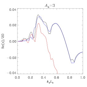
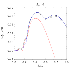
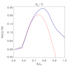
Figure 10: Linear stability of beams of different amplitudes. The largest growth rate of the Floquet eigenmodes, in units of $2\Omega$, is plotted versus the parallel wavenumber, in units of $L_{\mathrm{b}}^{-1}$, for beams of amplitudes $A_{\mathrm{b}}=2$, $3$, $4$ and $5$. The black lines are computed for a beam Ekman number of $Ek_{\mathrm{b}}=0.05$ and a periodic domain of width $L_{y}=40\pi\,L_{\mathrm{b}}$. The blue lines are for $Ek_{\mathrm{b}}=0.05$ and $L_{y}/L_{\mathrm{b}}=80\pi$, while the red lines are for $Ek_{\mathrm{b}}=0.1$ and $L_{y}/L_{\mathrm{b}}=40\pi$. Black crosses show growth rates estimated from numerical simulations with $Ek_{\mathrm{b}}=0.05$ and $L_{y}/L_{\mathrm{b}}=40\pi$. Note that the blue and black lines are often indistinguishable, indicating convergence of the growth rate with respect to the parameter $L_{y}/L_{\mathrm{b}}$.

The problem is determined by several dimensional parameters: $\Omega_{x}$, $\Omega_{y}$, $\nu$, $U_{0}$, $L_{\mathrm{b}}$, $k_{x}$ and $L_{y}$. We specialize to the case $\Omega_{x}=\Omega_{y}=\Omega/\sqrt{2}$ in which the beam propagates at an angle $\pi/4$ to the rotation axis, as in the global problem we consider. The beam is then described by two dimensionless parameters, the dimensionless beam amplitude

$$A_{\mathrm{b}}=\frac{U_{0}}{2\Omega L_{\mathrm{b}}}$$ (33)

and the beam Ekman number

$$Ek_{\mathrm{b}}=\frac{\nu}{2\Omega L_{\mathrm{b}}^{2}}.$$ (34)

The results of the linear calculation can be expressed by finding the dimensionless growth rate $s/2\Omega$ as a function of the dimensionless wavenumber $k_{x}L_{\mathrm{b}}$. The remaining dimensionless parameter is $L_{y}/L_{\mathrm{b}}$, which we aim to make as large as possible.

The maximum relative vorticity in the beam is $0.4514(U_{0}/L_{\mathrm{b}})$; this follows from $\max|g^{\prime}|=g^{\prime}(0)/\mathrm{i}={\textstyle\frac{1}{3}}\Gamma({\textstyle\frac{2}{3}})\approx 0.4514$. Both $x$ and $z$ components of the relative vorticity attain this maximum value. The maximum beam vorticity exceeds the vorticity $2\Omega$ associated with the background rotation when $A_{\mathrm{b}}>2.215$. (It may also be relevant for stability to compare the components of the beam vorticity in the direction of the rotation axis with $2\Omega$; then the beam exceeds the background when $A_{\mathrm{b}}>3.133$, which implies that Rayleigh’s criterion is violated near the centre of the beam at some phase of the oscillation.)

Sample results of our linear calculations are shown in Figure 10. For sufficiently large $A_{\mathrm{b}}$ the beam has a robust local instability, for values of $k_{x}L_{\mathrm{b}}$ somewhat less than unity, that is insensitive to $L_{y}$ for $L_{y}/L_{\mathrm{b}}\gg 1$. The maximum growth rate increases rapidly with $A_{\mathrm{b}}$. For smaller $A_{\mathrm{b}}$ weaker instabilities are found in periodic domains, but these depend significantly on $L_{y}$ and may vanish in the limit $L_{y}/L_{\mathrm{b}}\gg 1$. They probably involve parametric resonances with global inertial modes of the periodic domain, and rely on the artificial periodic repetition of the beam. For $A_{\mathrm{b}}=1$, there is no instability for $Ek_{\mathrm{b}}=0.05$ or $Ek_{\mathrm{b}}=0.1$.

We have verified the linear calculations and determined the nonlinear outcome of the instability of the beam through direct numerical simulations in which equations (28) and (29) are solved in a periodic box using a spectral method. The scaled box length $L_{x}/L_{\mathrm{b}}$ enters as an additional dimensionless parameter. The beam is initialized and maintained through a body force as described above. A very small random perturbation is added to the flow, either with a single wavenumber $k_{x}$ or a broad spectrum. The outcome of the simulations is in excellent agreement with the Floquet analysis regarding the growth rates of the unstable modes. Some of these growth rates are indicated as crosses in Figure 10. In cases with a strong instability, the transverse kinetic energy grows and saturates. The other two parts of the kinetic energy are reduced below their laminar values but are still greater than the transverse energy. We find that the temporal power spectrum is quite noisy but shows a main peak at the beam frequency and two smaller peaks at subharmonics close to half the primary wave frequency.

4.2 Parameters of the beams expected in the global wave attractor

In this section we estimate the dimensionless parameters of the inertial-wave beams expected to occur in the global wave attractor simulations on the basis of the linear asymptotic analysis of Ogilvie (2005). If we neglect the nonlinear terms in the basic equations (28) and (29), assume a time-dependence $\propto\mathrm{e}^{-\mathrm{i}\omega_{\mathrm{b}}t}$ and set to zero the force component $a_{z}$, then we obtain

$$-(-\mathrm{i}\omega_{\mathrm{b}}-\nu\nabla^{2})\nabla^{2}\psi-2{\bf{\Omega}}\cdot{\nabla}u_{z}=F_{0},$$ (35)

$$(-\mathrm{i}\omega_{\mathrm{b}}-\nu\nabla^{2})u_{z}-2{\bf{\Omega}}\cdot{\nabla}\psi=0,$$ (36)

where $F_{0}=\partial_{x}a_{y}-\partial_{y}a_{x}$. We select coordinates aligned with the attractor, in which one of the beams is centred on the line $y=0$, and $\omega_{\mathrm{b}}=2\Omega_{x}=2\Omega_{y}=\sqrt{2}\Omega$ as in the previous section. In this case our equations become

$$-(-\mathrm{i}\omega_{\mathrm{b}}-\nu\nabla^{2})\nabla^{2}\psi-\omega_{\mathrm{b}}(\partial_{x}+\partial_{y})u_{z}=F_{0},$$ (37)

$$(-\mathrm{i}\omega_{\mathrm{b}}-\nu\nabla^{2})u_{z}-\omega_{\mathrm{b}}(\partial_{x}+\partial_{y})\psi=0,$$ (38)

which may be combined into

$$(\mathrm{i}\omega_{\mathrm{b}}+\nu\nabla^{2})^{2}\nabla^{2}\psi+\omega_{\mathrm{b}}^{2}(\partial_{x}+\partial_{y})^{2}\psi=(\mathrm{i}\omega_{\mathrm{b}}+\nu\nabla^{2})F_{0}.$$ (39)

The viscous terms are important only in narrow beams. Expanding out the equation and retaining only the leading viscous terms, we obtain

$$2\omega_{\mathrm{b}}^{2}\partial_{x}\partial_{y}\psi+2\mathrm{i}\omega_{\mathrm{b}}\nu\nabla^{4}\psi=\mathrm{i}\omega_{\mathrm{b}}F_{0},$$ (40)

which can be written in the same form as the basic equation (3.1) of Ogilvie (2005),

$$\mathrm{i}\partial_{x}\partial_{y}\psi+\epsilon^{3}\nabla^{4}\psi=f,$$ (41)

if we identify

$$\epsilon^{3}=-\frac{\nu}{\omega_{\mathrm{b}}},\qquad f=-\frac{F_{0}}{2\omega_{\mathrm{b}}}.$$ (42)

As stated in Sect. 3.1 and according to Ogilvie (2005), the dominant ‘$n=0$’ part of the asymptotic inner solution close to the attractor is

$$\psi\sim a_{0}\chi_{0}(\tau)+b_{0},$$ (43)

where $b_{0}$ is an unimportant constant and $a_{0}$ and $\chi_{0}(\tau)$ were defined above (see Eqs 11 and 14). We recall that:

$$a_{0}=\frac{\delta}{\ln\alpha},\qquad\delta=-\mathrm{i}\int_{\mathrm{attractor}}f\,\mathrm{d}A,$$ (44)

that the function $\chi_{0}(\tau)$ is related to our function $g(\tau)$ through

$$\chi_{0}^{\prime}(-\tau)=\mathrm{i}g(\tau),$$ (45)

and that the scaled coordinate $\tau$ is defined as $\tau=y/L_{\mathrm{b}}$ where

$$L_{\mathrm{b}}=-\epsilon\mu^{1/3}=\left(\frac{\nu\mu}{\omega_{\mathrm{b}}}\right)^{1/3},$$ (46)

where $\mu$ is the distance along the beam from its virtual source, outside the fluid domain.

We therefore expect a velocity parallel to the beam of amplitude

$$U_{0}=-\frac{\mathrm{i}a_{0}}{L_{\mathrm{b}}}=\frac{F_{0}}{2\omega_{\mathrm{b}}L_{\mathrm{b}}\ln\alpha}\frac{5L^{2}}{9}.$$ (47)

The predicted dimensionless beam amplitude is then

$$A_{\mathrm{b}}=\frac{U_{0}}{2\Omega L_{\mathrm{b}}}=\frac{1}{2^{5/6}4\ln 2}\left(\frac{5}{9}\right)^{2/3}\left(\frac{\nu}{2\Omega L^{2}}\right)^{-2/3}\frac{F_{0}}{(2\Omega)^{2}}\left(\frac{\mu}{L_{\mathrm{a}}}\right)^{-2/3}$$ (48)

and the beam Ekman number is

$$Ek_{\mathrm{b}}=\frac{\nu}{2\Omega L_{\mathrm{b}}^{2}}=\left(\frac{9}{10}\right)^{1/3}\left(\frac{\nu}{2\Omega L^{2}}\right)^{1/3}\left(\frac{\mu}{L_{\mathrm{a}}}\right)^{-2/3}.$$ (49)

$L_{\mathrm{a}}$ is the length of one side of the attractor and is thus equal in the complete problem to $\sqrt{5/9}\,L$. Note that the dimensionless distance $\mu/L_{\mathrm{a}}$ along the beam ranges from $1/7$ to $8/7$, already showing that if the instability develops, it should start where the dimensionless amplitude is maximal and thus at the reflection points where $\mu/L_{\mathrm{a}}=1/7$. This is indeed where the subharmonics in our global attractor simulations seem to be excited first.

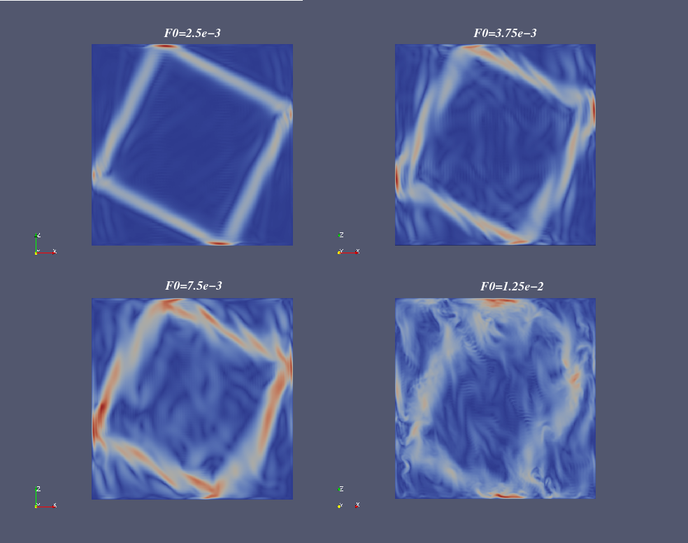
Figure 11: Snapshot of the norm of the velocity in the plane $\sqrt{v_{x}^{2}+v_{z}^{2}}$ in the statistically steady state for four different forcing amplitudes, from $F_{0}=2.5\times 10^{-3}$ to $F_{0}=1.25\times 10^{-2}$.

4.3 Instability of the primary wave attractor in the full non-linear simulations

Let us now come back to the direct numerical simulations of the global attractor which was studied in Section 3.1 in the linear regime. We are thus returning to the coordinate system defined in Section 2.1, in which coordinates $(x,z)$ are aligned with the container and $y$ is in the third direction. The two previous subsections indicate that an instability should be clearly visible when the equivalent beam Ekman number is around $Ek_{b}=0.05$. We choose to fix the value of $Ek={\nu}/{2\Omega L^{2}}$ to a value which was studied in the linear regime (i.e. $Ek=3.9\times 10^{-6}$), which, according to the previous subsection, translates into a beam Ekman number of $Ek_{b}\approx 0.0556$ at the reflection point where $\mu/L_{\mathrm{a}}=1/7$.

For this value of $Ek_{\mathrm{b}}$, the linear analysis above shows us that the first signs of a clear local instability should be seen for a beam amplitude of $A_{\mathrm{b}}\approx 4$, leading to a forcing amplitude around ${F_{0}}/{(2\Omega)^{2}}=2\times 10^{-3}$. Indeed, for $A_{\mathrm{b}}=1$, all the growth rates are negative and the threshold for instability is not reached yet. As shown in Fig. 10, when $A_{\mathrm{b}}=2$, the growth rates of possible unstable modes are extremely small (of the order of $70$ wave periods) and the instability thus likely not to be seen in our global simulations. On the contrary when we reach the value of $A_{\mathrm{b}}\approx 4$, a clear instability is present in the linear analysis as seen in the two bottom panels of Fig. 10. We have not tried to determine precisely the threshold for instability in the global simulations, but we wish to determine whether we get some clear signs of instability when we force the system with ${F_{0}}/{(2\Omega)^{2}}\geq 2\times 10^{-3}$.

We show in Fig. 11 the norm of the velocity $(v_{x},0,v_{z})$ in the $(x,z)$-plane for increasing values of the forcing amplitude, for an Ekman number $Ek=3.9\times 10^{-6}$. The four snapshots were chosen at a time when both the power input and the dissipation rate have reached a statistically steady state and at a temporal phase close to $t=0$ (i.e. when the parallel velocity is positive and maximum). As seen in this figure, as the forcing amplitude is increased, the spatial structure of the beam is perturbed and starts to be modified mostly at the locations of reflections, i.e. at the corners of the attractor. At $F_{0}=3.75\times 10^{-3}$ and $F_{0}=7.5\times 10^{-3}$, we start to distinguish waves propagating at different angles with respect to the rotation vector, indicating the potential existence of excitation at different frequencies, as will be presented later. In the case with the largest forcing amplitude ($F_{0}=1.25\times 10^{-2}$), the attractor is hardly visible since the kinetic energy is much less concentrated than in the previous cases. The wave focusing is in this case less efficient. The primary wave beam is nonetheless still distinguishable but tends to be broader and more affected by the surrounding velocity field. It is then clear that the attractor is strongly affected by the nonlinearities and filters will have to be applied to distinguish the spatial structure of the beam in these cases. We make use of the procedure of Grisouard et al. (2008) to correctly visualize the beam in the nonlinear cases. We choose to filter the $z$ and the $y$-components of the velocity at the frequency of the forcing term first and then at various subharmonics to observe the spatial structure at each of those frequencies. Our filtered field at frequency $\omega$ thus takes the following expression:

$${\bf V}_{\omega}(x,z)=\frac{\omega}{N\pi}\,\,\int_{t_{\mathrm{i}}}^{t_{\mathrm{f}}}\,\,{\bf v}(x,z,t)\exp[\mathrm{i}\,\omega(t-t_{\mathrm{i}})]\,\mathrm{d}t.$$ (50)

where $t_{\mathrm{i}}$ is taken in the well-established steady state at about $500$ wave periods $(T=2\pi/\omega_{0})$ after initialization and $t_{\mathrm{f}}$ is taken $N\approx 100$ wave periods later.

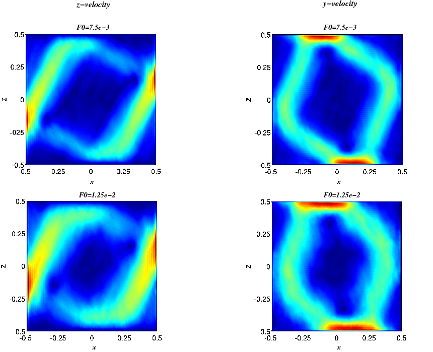
Figure 12: Modulus of the filtered velocity field at $\omega_{0}=\sqrt{2}\Omega$ for the cases where the amplitude of the forcing is equal to $F_{0}=7.5\times 10^{-3}$ and $F_{0}=1.25\times 10^{-2}$ and with $Ek=3.9\times 10^{-6}$.

Figure 12 shows the result of the filtering of $v_{z}$ and $v_{y}$ at the forcing frequency $\omega_{0}$ in two cases, namely when the forcing amplitude is set to $7.5\times 10^{-3}$ and when it is set to $1.25\times 10^{-2}$. The latter case corresponds to the last panel of Fig. 11 where the beam was clearly strongly perturbed by the nonlinearities. The filtering procedure thus enables us to recover the spatial structure of the primary beam, i.e. at the forcing frequency. One striking feature here is that the effective thickness of the attractor increases in the nonlinear cases, indicating that instability and nonlinear dynamical processes prevent the waves from focusing on very short scales.

When the energy balance is investigated, we find again in those nonlinear cases that in the statistically steady state, the dissipation rate is on average equal to the power input from the body force, with an error of a few percent that may be due to the effects of the mask as in the linear regime.

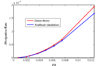
Figure 13: Blue curve: dissipation rate computed for various forcing amplitudes (from 16). Red curve: dissipation rate predicted by linear theory (from 17), which scales with $F_{0}^{2}$.

However, there is a difference in the nonlinear cases in the time it takes for the dissipation rate to saturate to its final value. Indeed, when the forcing amplitude is increased, it takes less time for the dissipation rate to saturate, which is related to the fact that the final beam becomes broader, as seen in Fig. 12. When the forcing is stronger, it thus seems that the kinetic energy reaches the dissipative scales more rapidly by an instability mechanism than it does purely by geometrical focusing. As a consequence, the level of saturation for the dissipation rate is reached before the waves have time to focus on the attractor and the spatial structure of the wave beam is strongly modified. The dissipation rate is computed for the cases with $F_{0}=7.5\times 10^{-4},2\times 10^{-3},10^{-2},3.75\times 10^{-3},5\times 10^{-3},6.25\times 10^{-3},7.5\times 10^{-3}$ and $1.25\times 10^{-2}$ and compared to the asymptotic linear value calculated in the previous section. Figure 13 shows the values of the dissipation rate as a function of the forcing amplitude $F_{0}$ (blue curve) and the asymptotic values found in the linear theory (red curve). We find an agreement between the two curves of around $95\%$ for the first three points, where the nonlinear effects are limited. The agreement then decreases to $92\%$ for the four following values and then drops to $85\%$ for the last case which corresponds to $F_{0}=1.25\times 10^{-2}$. In the latter case, the strong nonlinear effects prevent the waves from focusing on the short scale of the theoretical attractor. The instability of the wave beam provides here another way to transfer energy to smaller and smaller wavelengths until they reach the dissipative scale.

4.4 Non linear outcome of the instability in the global simulations

Since it is clearly visible in Fig. 11 that the structure of the flow changes with increasing amplitude of the forcing applied to the system, we need to focus on the temporal power spectrum of the velocity, in order to have a precise idea of which frequencies are excited in the domain. Fig. 14 shows the spectra of one component of the velocity ($v_{z}$) at a particular point in the attractor, for a forcing amplitude varying from $F_{0}=2\times 10^{-3}$ to $F_{0}=3.75\times 10^{-3}$ and keeping $Ek=3.9\times 10^{-6}$. All spectra are superimposed so that we can clearly analyse which frequencies appear for which forcing amplitude. In the linear case at $F_{0}=2\times 10^{-3}$, the only visible peak is the one at the forcing frequency $\omega=\omega_{0}=\sqrt{2}/2$. This peak of highest amplitude is present for all cases we have computed. This also explains why the spatial structure of the attractor could still be recovered even for the relatively high forcing amplitude of $F_{0}=1.25\times 10^{-2}$.

When the forcing is increased and thus when the simulations become more and more nonlinear, additional frequencies are excited, especially at lower values. It seems that the instability here transfers energy from the primary wave to two recipient waves at lower frequencies. This was also found in laboratory experiments where internal gravity waves were excited (Joubaud et al., 2012).

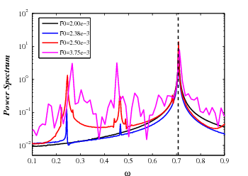
Figure 14: Power spectrum of the kinetic energy for cases at various forcing amplitudes, as a function of frequency $\omega$ and for $Ek=3.9\times 10^{-6}$. The vertical dashed line shows the location of the primary wave frequency $\omega_{0}=\sqrt{2}\Omega=\sqrt{2}/2$.

As the forcing amplitude increases and the nonlinearities become even more important, these subharmonics tend to get closer to half the primary wave frequency. The resonance condition for the frequencies remains true in those more nonlinear cases. This is mostly visible in the case where $F_{0}=3.75\times 10^{-3}$ in which the peaks at low frequencies move closer to $\omega_{0}/2=\sqrt{2}/4$. This can be explained by the fact that as the forcing amplitude is increased, the Reynolds number of the flow becomes larger and the instability behaves as if the viscosity was reduced. The characteristics of the instability thus become closer and closer to the inviscid case: shorter secondary waves with a frequency close to half the primary wave frequency, in agreement with the dispersion relation of such inertial waves.

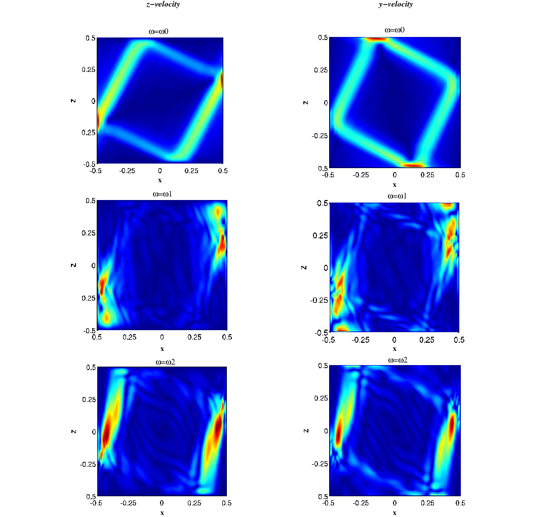
Figure 15: Filtered velocity field ($z$ and $y$ components) for the case with a forcing amplitude of $F_{0}=2.5\times 10^{-3}$. The filtering is made at the 3 principal frequencies visible in the power spectrum, namely $\omega_{0}=\sqrt{2}/2$, $\omega_{1}=0.244$ and $\omega_{2}=0.463$.

It is then interesting to use the same procedure as the previous section to filter the velocity field not at the primary frequency $\omega_{0}$ like we did to get the spatial structure of the main attractor, but at the subharmonic frequencies, namely at $\omega_{1}$ and $\omega_{2}$. The results are shown in Fig. 15 for the case at $F_{0}=2.5\times 10^{-3}$, where the frequencies of the subharmonics clearly appear in the power spectrum of Fig. 14.

In Fig. 15, six panels are represented, showing the filtering of the $z$ and the $y$-components of the velocity at the frequency of the primary wave $\omega_{0}$, and at the frequencies where the Fourier transform shows a signal, namely at $\omega_{1}\approx 0.244$, $\omega_{2}\approx 0.463$. Those values correspond approximately to $\omega_{1}/\omega_{0}=0.345$ and $\omega_{2}/\omega_{0}=0.655$. On the top panels, the regular spatial structure of the initial attractor is recovered, with a typical thickness slightly larger than in the linear simulations. On the next two panels, it seems that the secondary waves are excited within the primary wave attractor in a region where the energy of the primary wave is maximum (i.e. close to the walls where the reflections occur). The secondary waves then propagate with a different angle with respect to the rotation vector compared to the primary wave. This is due to the dispersion relation of such inertial waves which implies that the angle between the rotation vector and the direction of propagation depends directly on the wave frequency. Since those waves have smaller wavelengths than the primary wave, they also dissipate more quickly and thus do not propagate very far away from their region of excitation. This is especially true for the waves excited at $\omega_{1}$. Indeed, the mid-panels show a strong location of kinetic energy at this frequency close to the region of excitation but the structure stays spatially localized very close to the corners of the attractor. This is less true for the waves excited at the higher frequency $\omega_{2}$ which clearly exhibit a region of propagation along a beam inclined at an angle $\theta_{2}$ with respect to the rotation vector, such that $\sin\theta_{2}=\omega_{2}/2\Omega$.

5 Summary and conclusion

The purpose of this work was to simulate numerically the evolution in 2D of an inertial wave attractor in a square container in the linear and nonlinear regimes, with a particular focus on the build-up of the attractor before it reaches a steady-state and the instability occurring in the nonlinear case. This study complements previous work on this problem, namely laboratory experiments and linear calculations. In the linear regime, the characteristics of internal wave attractors predicted by theory are well recovered. In particular, we find that the thickness of the attractor scales with the Ekman number to the power $1/3$. For a fixed Ekman number, we moreover confirm that after a reflection at the boundary, the amplitude of the velocity field decreases as the distance from the source to the power $1/3$ while the breadth of the wave beam increases by the same factor. Finally, we find in the simulations that, for a body force of fixed amplitude, the dissipation rate indeed becomes independent of the Ekman number and approaches the asymptotic value derived analytically in Ogilvie (2005).

Since we compute the evolution of the wave attractor from the very beginning where an incompressible fluid is forced in a closed container, we have access to the transient phase before the system reaches a statistically steady state. In this simple linear case, only two quantities will play a role in the energy balance: the power input due to the periodic forcing of the system and the dissipation rate. Both those quantities reach the same absolute value in the steady state in order for energy to be conserved. However, we find here that the power (i.e. the rate of working by the applied force) saturates in about 5 wave periods in all cases, while the dissipation rate reaches its asymptotic value on a timescale that depends on the Ekman number, typically close to 15 wave periods. The kinetic energy of the flow therefore continues to build up, and the dissipation rate increases, until the wave attractor has reached its final thickness, while the rate of working by the applied force saturates much earlier. This is consistent with the viewpoint that the attractor acts as a “black hole” that absorbs the energy flux associated with the quasi-inviscid, large-scale waves that are focused towards it.

The present work also focused on the properties of inertial wave attractors in the nonlinear regimes. To do so, the forcing amplitude was increased until nonlinear effects would start to play a significant role. The primary wave beam oscillating at the forcing frequency $\omega_{0}$ is then found to be subject to an instability which is investigated through linear analysis and nonlinear calculations of the simpler case of a single infinite narrow wave beam. The onset of this instability and the nonlinear outcome are determined in this simpler case and are consistent with the characteristics of the global wave attractor in the nonlinear regime. It is found that this instability transfers energy to waves of lower frequencies and shorter wavelengths. Those secondary inertial waves are excited close to the reflection points and then propagate with a direction in agreement with the typical inertial wave dispersion relation. Since they possess a smaller scale, they dissipate quickly and propagate over much shorter distances than the primary waves. As the forcing amplitude is increased, their effective Reynolds number is increased and the frequencies of the secondary waves drift towards $\omega_{0}/2$, thus approaching the outcome of a regular parametric subharmonic instability in the inviscid case. In the cases where instability occurs, the energy is transferred rapidly to shorter wavelengths which then dissipate. As a consequence, the dissipation rate reaches its saturation more quickly than in the linear cases. In the present work, this type of instability is described theoretically and recovered in nonlinear direct numerical simulations. An instability of a wave beam with similar characteristics was found in an experiment and supported by nonlinear numerical simulations by Clark & Sutherland (2010). Other types of instabilities were also observed in laboratory experiments of gravity waves (Joubaud et al., 2012) or inertial waves (Bordes et al., 2012) excited in closed containers.

In geophysical or astrophysical situations, inertial waves can be excited in stars or planets by tidal forcing due to an orbiting companion. Moreover, these systems can easily be in a nonlinear regime if the forcing is sufficiently strong (because of the companion being sufficiently close and/or massive). Under these conditions, wave attractors can still be present but the flow may be unstable and the dissipation rate and tidal torque may be reduced below the value predicted by linear theory.

Of course the problem considered here was 2D, consisting of a very simple geometry and it has been shown that moving to 3D and spherical geometry may strongly modify the behaviour of wave attractors and the characteristics of the dissipation processes (Rieutord & Valdettaro, 2010). However, it is the first example here of strong nonlinear effects emerging in simulations of wave attractors, namely subharmonic instabilities. It is interesting to note that our simulations have counterparts in the recent fluid experiments of Scolan et al. (2013), which also exhibit a strongly nonlinear regime of wave attractors.

Obviously, much more can be done on this problem. If we consider the conditions in the interiors of stars or giant planets, large-scale flows such as meridional flows or differential rotation are likely to exist and modify the build-up of potential wave attractors. Turbulent convection will of course also probably act on the wave focusing and defocusing and may disrupt the formation of wave attractors. A next possible step could be the computation of the same kind of simulations for a compressible fluid in a rotating spherical shell, where both gravity and inertial waves would exist. In spherical geometry, critical latitude singularities were shown to be dominant features of periodically forced flows in a linear regime. It would be valuable to carry out fully nonlinear simulations of these phenomena.