Transition probabilities in the $U(3,3)$ limit of the symplectic IVBM

Abstract

The tensor properties of the algebra generators are determined in respect to the reduction chain $Sp(12,R)\supset U(3,3)\supset U_{p}(3)\otimes\overline{U_{n}(3)}\supset U^{\ast}(3)\supset O(3)$, which defines one of the dynamical symmetry limits of the Interacting Vector Boson Model (IVBM). The symplectic basis according to the considered chain is thus constructed and the action of the $Sp(12,R)$ generators as transition operators between the basis states is illustrated. The matrix elements of the $U(3,3)$ ladder operators in the so obtained symmetry-adapted basis are given. The $U(3,3)$ limit of the model is further tested on the more complicated and complex problem of reproducing the $B(E2)$ transition probabilities between the collective states of the ground band in ${}^{104}Ru$, ${}^{192}Os$, ${}^{192}Pt$, and ${}^{194}Pt$ isotopes, considered by many authors to be axially asymmetric. Additionally, the excitation energies of the ground and $\gamma$ bands in ${}^{104}Ru$ are calculated. The theoretical predictions are compared with the experimental data and some other collective models which accommodate the $\gamma-$rigid or $\gamma-$soft structures. The obtained results reveal the applicability of the model for the description of the collective properties of nuclei, exhibiting axially asymmetric features.

PACS 21.60.Fw, 23.20.-g, 21.10.Re, 27.80.+w, 27.60.+j

I Introduction

Symmetry is an important concept in physics. In finite many-body systems, it appears as time reversal, parity, and rotational invariance, but also in the form of dynamical symmetries DG -RW . In the algebraic models, the use of the dynamical symmetries defined by a certain reduction chain of the group of dynamical symmetry yields exact solutions for the eigenvalues and eigenfunctions of the model Hamiltonian, which is constructed from the invariant operators of the subgroups in the chain. Many properties of atomic nuclei have been investigated using such models, in which one obtains bands of collective states which span irreducible representations of the corresponding dynamical groups.

Something more, it is very simple and straightforward to calculate the matrix elements of transition operators between the eigenstates as both - the basis states and the operators - can be defined as tensor operators in respect to the considered dynamical symmetry. Then the calculation of matrix elements is simplified by the use of a respective generalization of the Wigner-Eckart theorem, which requires the calculation of the isoscalar factors and reduced matrix elements. By definition such matrix elements give the transition probabilities between the collective states attributed to the basis states of the Hamiltonian.

The comparison of the experimental data with the calculated transition probabilities is one of the best tests of the validity of the considered algebraic model. With the aim of such applications of one of the dynamical symmetries of the symplectic Interacting Vector Boson Model (IVBM), we develop in this paper a practical mathematical approach for explicit evaluation of the matrix elements of transitional operators in the model.

The IVBM and its recent applications for the description of diverse collective phenomena in the low-lying energy spectra (see, e.g., the review article pepan ) exploit the symplectic algebraic structures and the Sp(12,$R$) is used as a dynamical symmetry group. Symplectic algebras and their substructures have been applied extensively in the theory of nuclear structure GL -Vanagas . They are used generally to describe systems with a changing number of particles or excitation quanta and in this way provide for larger representation spaces and richer subalgebraic structures that can accommodate the more complex structural effects as realized in nuclei with nucleon numbers that lie far from the magic numbers of closed shells. In particular, the model approach was adapted to incorporate the newly observed higher collective states, both in the first positive and negative parity bands Sp12U6 by considering the basis states as ”yrast” states for the different values of the number of bosons $N$ that built them.

In Ref.TSIVBM a new dynamical symmetry limit of the IVBM was introduced, which seems to be appropriate for the description of deformed even-even nuclei, exhibiting triaxial features. Usually, in the geometrical approach the triaxial nuclear properties are interpreted in terms of either the $\gamma$-unstable rotor model of Wilets and Jean WJ or the rigid triaxial rotor model (RTRM) of Davydov et al. DF . An alternative description can be achieved by exploiting the properties of the $SU^{\ast}(3)$ algebra introduced in Ref.TSIVBM (and appearing also in the context of IBM-2 PSDiep ). The latter is appropriate for nuclei in which the one type of particles is particle-like and the other is hole-like. Using a schematic Hamiltonian with a perturbed $SU^{\ast}(3)$ dynamical symmetry, the IVBM was applied for the calculation of the low-lying energy spectrum of the nucleus ¹⁹²Os TSIVBM . The obtained results proved the relevance of the proposed dynamical symmetry in the description of deformed triaxial nuclei.

In this paper we develop further our theoretical approach initiated in Ref.TSIVBM by considering the transition probabilities in the framework of the symplectic IVBM with $Sp(12,R)$ as a group of dynamical symmetry. For this purpose we consider the tensorial properties of the algebra generators in respect to the reduction chain:

(6)

where $U_{p}(3)$ and $\overline{U_{n}(3)}$ are the one-fluid algebras corresponding to the two nuclear subsystems, $U^{\ast}(3)$ is the combined two-fluid algebra, and $SO(3)$ is the standard angular momentum algebra. Further we classify the basis states by the quantum numbers corresponding to the irreducible representations (irreps) of different subgroups along the chain (6). In this way we are able to define the transition operators between the basis states and then to evaluate analytically their matrix elements. This will allow us further to test the model in the description of the electromagnetic properties observed in some non-axial nuclei. As a first step we will test the theory on the transitions between the states belonging to the ground state bands (GSB) in some even-even nuclei from the $A\approx 100$ and $A\approx 190$ mass regions.

II Tensorial properties of the generators of the Sp(12,R) group

It was suggested by Bargmann and Moshinsky BargMosh that two types of bosons are needed for the description of nuclear dynamics. It was shown there that the consideration of only two-body system consisting of two different interacting vector particles will suffice to give a complete description of $N$ three-dimensional oscillators with a quadrupole-quadrupole interaction. The latter can be considered as the underlying basis in the algebraic construction of the phenomenological IVBM.

The basic building blocks of the IVBM TSIVBM are the creation and annihilation operators of two kinds of vector bosons $u_{m}^{{\dagger}}(\alpha)$ and $u_{m}(\alpha)$ $(m=0,\pm 1)$, which differ in an additional quantum number $\alpha=\pm 1/2$ (or $\alpha=p$ and $n$)$-$the projection of the $T$-spin (an analogue to the $F$-spin of IBM-2 or the $I$-spin of the particle-hole IBM). In the present paper, we consider these two bosons just as elementary building blocks or quanta of elementary excitations (phonons) rather than real fermion pairs, which generate a given type of algebraic structures. Thus, only their tensorial structure is of importance and they are used as an auxiliary tool, generating an appropriate dynamical symmetry.

The vector bosons can be considered as components of a $6-$dimensional vector, which transform according to the fundamental $U(6)$ irreducible representation $[1,0,0,0,0,0]_{6}\equiv[1]_{6}$ and its conjugate (contragradient) one $[0,0,0,0,0,-1]_{6}\equiv[1]_{6}^{\ast}$, respectively. These irreducible representations become reducible along the chain of subgroups (6) defining the dynamical symmetry. This means that along with the quantum number characterizing the representations of $U(6)$, the operators are also characterized by the quantum numbers of the subgroups of chain (6). Introducing the notations $u_{i}^{{\dagger}}(\frac{1}{2})=p_{i}^{{\dagger}}$ and $u_{i}^{{\dagger}}(-\frac{1}{2})=n_{i}^{{\dagger}}$, the components of the creation operators $u_{m}^{{\dagger}}(\alpha)$ labeled by the chain (6) can be written as:

$$p^{{\dagger}}_{m}\equiv p^{{{\dagger}}[1]_{6}}_{[1]_{3}[0]^{\ast}_{3}\ [1]_{3}(1)_{3}m},\ \ \ n^{{\dagger}}_{m}\equiv n^{{{\dagger}}[1]_{6}}_{[0]_{3}[1]^{\ast}_{3}\ [1]^{\ast}_{3}(1)_{3}m}.$$ (7)

According to the chain (6), the fundamental $U(6)$ irrep $[1]_{6}$ decomposes as

$$[1]_{6}\supset[1]_{3}\oplus[1]^{\ast}_{3},$$ (8)

i.e. as a direct product sum of the $U_{p}(3)$ and $\overline{U_{n}(3)}$ fundamental irreps. In Eq.(8) the $[1]^{\ast}_{3}$ denotes the (contragradient) irrep of $\overline{U_{n}(3)}$ which is conjugate to the $[1]_{3}$ of $U_{p}(3)$. This corresponds to the case when the one type of particles in the two-fluid nuclear system is particle-like and the other is hole-like. Note that there is an alternative decomposition of the fundamental $U(6)$ irrep $[1]_{6}$:

$$[1]_{6}\supset[1]_{3}\oplus[1]_{3},$$ (9)

where the group $\overline{U_{n}(3)}$ in Eq.(6) should be replaced by the $U_{n}(3)$ one. The decomposition (9) is appropriate for the situation when the nucleus is considered as consisting of two particle-like constituents. In our further considerations we will need also the reduction of the $U(6)$ irrep $[2]_{6}$ along the chain (6). According to the decomposition rules for the fully symmetric $U(6)$ irreps, we obtain for the $U_{p}(3)\otimes\overline{U_{n}(3)}$ content

$$[2]_{6}\supset[2]_{3}[0]^{\ast}_{3}+[1]_{3}[1]^{\ast}_{3}+[0]_{3}[2]^{\ast}_{3}.$$ (10)

Thus, the generators of the symplectic group $Sp(12,R)$ can already be defined as irreducible tensor operators according to the whole chain (6) of subgroups as follows.

The raising operators of $Sp(12,R)$ can be expressed as

$$F_{[\lambda]_{3}[0]_{3}^{\ast}\quad[\lambda]_{3}}^{\quad[\chi]_{6}\quad LM} =C_{[1]_{3}[0]_{3}^{\ast}\quad[1]_{3}[0]^{\ast}_{3}\quad[\lambda]_{3}[0]^{\ast}_{3}}^{[1]_{6}\quad\quad[1]_{6}\quad\quad\quad[\chi]_{6}}C^{[\lambda]_{3}}_{[1]_{3},[1]_{3}}$$

$$\times C_{(1)_{3}(1)_{3}(L)_{3}}^{[1]_{3}[1]_{3}[\lambda]_{3}}C_{1m1n}^{LM}$$

$$\times p^{{{\dagger}}[1]_{6}}_{[1]_{3}[0]^{\ast}_{3}\ [1]_{3}(1)_{3}m}p^{{{\dagger}}[1]_{6}}_{[1]_{3}[0]^{\ast}_{3}\ [1]_{3}(1)_{3}n},$$ (11)

$$F_{[0]_{3}[\lambda]_{3}^{\ast}\quad[\lambda]^{\ast}_{3}}^{\quad[\chi]_{6}\quad LM} =C_{[0]_{3}[1]_{3}^{\ast}\quad[0]_{3}[1]^{\ast}_{3}\quad[0]_{3}[\lambda]^{\ast}_{3}}^{[1]_{6}\quad\quad[1]_{6}\quad\quad\quad[\chi]_{6}}C^{[\lambda]_{3}}_{[-1]_{3},[-1]_{3}}$$

$$\times C_{(1)_{3}(1)_{3}(L)_{3}}^{[1]^{\ast}_{3}[1]^{\ast}_{3}[\lambda]^{\ast}_{3}}C_{1m1n}^{LM}$$

$$\times n^{{{\dagger}}[1]_{6}}_{[0]_{3}[1]^{\ast}_{3}\ [1]^{\ast}_{3}(1)_{3}m}n^{{{\dagger}}[1]_{6}}_{[0]_{3}[1]^{\ast}_{3}\ [1]^{\ast}_{3}(1)_{3}n},$$ (12)

$$F_{[1]_{3}[1]_{3}^{\ast}\quad[\lambda]_{3}}^{\quad[\chi]_{6}\quad LM} =C_{[1]_{3}[0]_{3}^{\ast}\quad[0]_{3}[1]^{\ast}_{3}\quad[0]_{3}[\lambda]_{3}}^{[1]_{6}\quad\quad[1]_{6}\quad\quad\quad[\chi]_{6}}C^{[\lambda]_{3}}_{[1]_{3},[-1]_{3}}$$

$$\times C_{(1)_{3}(1)_{3}(L)_{3}}^{[1]_{3}[1]^{\ast}_{3}[\lambda]_{3}}C_{1m1n}^{LM}$$

$$\times p^{{{\dagger}}[1]_{6}}_{[1]_{3}[0]^{\ast}_{3}\ [1]_{3}(1)_{3}m}n^{{{\dagger}}[1]_{6}}_{[0]_{3}[1]^{\ast}_{3}\ [1]^{\ast}_{3}(1)_{3}n},$$ (13)

where, according to the lemma of Racah Racah , the Clebsch-Gordan coefficients along the chain are factorized by means of the isoscalar factors (IF), defined for each step of decomposition (6). The lowering operators $G_{[\lambda^{\prime}]_{3}[\lambda^{\prime\prime}]_{3}\quad[\lambda]_{3}}^{\quad[\chi]_{6}\quad\quad LM}$ of $Sp(12,R)$ are obtained from the rasing ones $F_{[\lambda^{\prime}]_{3}[\lambda^{\prime\prime}]^{{\dagger}}_{3}\quad[\lambda]_{3}}^{\quad[\chi]_{6}\quad\quad LM}$ by Hermition conjugation. That is why we consider only the tensor properties of the raising operators.

The tensors (11)-(13) transform according to

$$[1]_{6}\times[1]_{6}=[2]_{6}+[1,1]_{6},$$ (14)

and their Hermition conjugate counterparts according to

$$[1]_{6}^{\ast}\times[1]_{6}^{\ast}=[-2]_{6}+[-1,-1]_{6},$$ (15)

respectively. But, since the basis states of the IVBM are fully symmetric, we consider only the fully symmetric $U(6)$ representation $[2]_{6}$ and its conjugate $[-2]_{6}$. Hence, the tensors (11)-(13) transform according to the $U(6)$ irrep $[\chi]_{6}\equiv[2]_{6}$.

The tensor (11) with respect to the $U^{\ast}(3)$ subgroup transforms according to the direct product

$$[1]_{3}\times[1]_{3}=[2]_{3}+[1,1]_{3},$$ (16)

while (12) and (13) transform according to

$$[1]^{\ast}_{3}\times[1]^{\ast}_{3}=[2,2]_{3}+[2,1,1]_{3}=[-2]_{3}+[1]_{3},$$ (17)

$$[1]_{3}\times[1]^{\ast}_{3}=[2,1]_{3}+[1,1,1]_{3}=[1,-1]_{3}+[0]_{3}$$ (18)

and obviously, because of their symmetric character, (11) and (12) transform only according to the symmetric $U^{\ast}(3)$ representations $[2]_{3}$ and $[-2]_{3}$, respectively. The latter follows also from the reduction (10). In this way we obtain the following set of raising generators:

$$F_{[2]_{3}[0]_{3}^{\ast}\quad[2]_{3}}^{\quad[2]_{6}\quad LM},\quad F_{[0]_{3}[2]_{3}^{\ast}\quad[-2]_{3}}^{\quad[2]_{6}\quad LM},$$ (19)

$$F_{[1]_{3}[1]_{3}^{\ast}\quad[2,1,0]_{3}}^{\quad[2]_{6}\quad LM},\quad F_{[1]_{3}[1]_{3}^{\ast}\quad[0]_{3}}^{\quad[2]_{6}\quad LM},$$ (20)

which together with their conjugate (lowering) operators change the number of bosons $N$ by two. The operators (20) and their conjugate counterparts are the ladder generators of $U(3,3)$ algebra.

In terms of Elliott’s notations Elliott $\left(\lambda,\mu\right)$, we have $[2]_{3}=(2,0)$, $[2]^{\ast}_{3}=[-2]_{3}=(0,2)$, $[210]_{3}=(1,1)$ and $[0]_{3}=(0,0)$. The corresponding values of $L$ from the $SU(3)\supset O(3)$ reduction rules are $L=0,2$ in both the $(2,0)$ and $(0,2)$ irreps, $L=1,2$ in the $(1,1)$ irrep and $L=0$ in the $(0,0)$.

The number preserving operators transform according to the direct product $[\chi]_{6}$ of the corresponding $U(6)$ representations $[1]_{6}$ and $[1]_{6}^{\ast}$, namely

$$[1]_{6}\times[1]_{6}^{\ast}=[1,-1]_{6}+[0]_{6},$$ (21)

where $[1,-1]_{6}=[2,1,1,1,1,0]_{6}$ and $[0]_{6}=[1,1,1,1,1,1]_{6}$ is the scalar $U(6)$ representation. They generate the maximal compact subgroup $U(6)$ of $Sp(12,R)$.

The tensor operators

$$A_{[\lambda]_{3}[0]^{\ast}_{3}\quad[\lambda]_{3}}^{[1-1]_{6}\quad LM}\simeq\frac{1}{\sqrt{2}}\sum_{m,k}C_{1m1k}^{LM}p_{m}^{{\dagger}}p_{k}$$ (22)

$$A_{[0]_{3}[\lambda]^{\ast}_{3}\quad[\lambda]^{\ast}_{3}}^{[1-1]_{6}\quad LM}\simeq\frac{1}{\sqrt{2}}\sum_{m,k}C_{1m1k}^{LM}\ n_{m}^{{\dagger}}n_{k}$$ (23)

correspond to the generators of the $U_{p}(3)$ and $\overline{U_{n}(3)}$ algebras, respectively. The operators with $L=1$ represent the angular momentum components, whereas those with $L=2$ correspond to the quadrupole momentum operators and together they generate the one-fluid $SU_{\tau}(3)$ ($\tau=p,n$) algebra. The tensors (22), (23) together with (20) and their conjugate counterparts, in turn, constitute the full set of $U(3,3)$ generators.

The linear combination operators

$$A^{\prime LM}_{[\lambda]_{3}}=A^{[1-1]_{6}\quad LM}_{[\lambda]_{3}[0]^{\ast}_{3}\quad[\lambda]_{3}}-(-1)^{L}A^{[1-1]_{6}\quad LM}_{[0]_{3}[\lambda]^{\ast}_{3}\quad[\lambda]_{3}}$$ (24)

generate the $U^{\ast}(3)$ algebra. The $SU^{\ast}(3)$ algebra is obtained by excluding the operator $A^{\prime 00}=N_{p}-N_{n}=M$ which is the single generator of the $O(2)$ algebra, whereas the angular momentum algebra $SO(3)$ is generated by the generators $A^{\prime 1M}\equiv L_{M}=L^{p}_{M}+L^{n}_{M}$ only. The operator $M$, counting the difference between particle and holes, is also the first order Casimir of $U(3,3)$ algebra and it decomposes the action space $\mathcal{H}$ of the $Sp(12,R)$ generators to the ladder ${\mathcal{H}}_{\nu}$ subspaces of the boson representations of $Sp(12,R)$ with $\nu=N_{p}-M_{n}=\pm 0,\pm 2,\pm 4,\ldots$ Sp2NRbr .

Finally, the tensors

$$A^{[1-1]_{6}\quad LM}_{[1]_{3}[1]_{3}\quad[\lambda]_{3}}\simeq\frac{1}{\sqrt{2}}\sum_{m,k}C_{1m1k}^{LM}\ p_{m}^{{\dagger}}n_{k},$$ (25)

$$A^{[1-1]_{6}\quad LM}_{[1]^{\ast}_{3}[1]^{\ast}_{3}\quad[\lambda]_{3}}\simeq\frac{1}{\sqrt{2}}\sum_{m,k}C_{1m1k}^{LM}\ n_{m}^{{\dagger}}p_{k}$$ (26)

with $L=0,1,2$ and $M=-L,-L+1,...,L$ extend the $U_{p}(3)\otimes\overline{U_{n}(3)}$ algebra to the $U(6)$ one.

In this way we have listed all the irreducible tensor operators in respect to the reduction chain (6) that correspond to the infinitesimal operators of the $Sp(12,R)$ algebra.

III Construction of the symplectic basis states of IVBM

Next, we can introduce the tensor products

$$T^{([\chi_{1}]_{6}[\chi_{2}]_{6})\quad\omega[\chi]_{6}}_{[\lambda_{1}]_{3}[\lambda_{2}]_{3}\quad\quad[\lambda]_{3}\quad\quad LM}=$$

$$\sum T^{[\chi_{1}]_{6}\quad\quad L_{1}M_{1}}_{[\lambda_{1}^{\prime}]_{3}[\lambda_{1}^{\prime\prime}]^{\ast}_{3}\ [\lambda_{1}]_{3}}T^{[\chi_{2}]_{6}\quad\quad L_{2}M_{2}}_{[\lambda_{2}^{\prime}]_{3}[\lambda_{2}^{\prime\prime}]^{\ast}_{3}\ [\lambda_{2}]_{3}}$$

$$\times C^{[\chi_{1}]_{6}\quad\quad\quad[\chi_{2}]_{6}\quad\quad\quad\omega[\chi]_{6}}_{[\lambda_{1}^{\prime}]_{3}[\lambda_{1}^{\prime\prime}]^{\ast}_{3}\quad[\lambda_{2}^{\prime}]_{3}[\lambda_{2}^{\prime\prime}]^{\ast}_{3}\quad[\lambda_{1}]_{3}[\lambda_{2}]_{3}}$$

$$\times C^{[\lambda]_{3}}_{[\lambda_{1}]_{3},[\lambda_{2}]_{3}}C^{[\lambda_{1}]_{3}\quad[\lambda_{2}]_{3}\quad[\lambda]_{3}}_{K_{1}L_{1}\ K_{2}L_{2}\quad KL}C^{L_{1}\quad L_{2}\quad L}_{M_{1}\quad M_{2}\quad M}$$ (27)

of two tensor operators $T^{[\chi_{i}]_{6}\quad\quad L_{i}M_{i}}_{[\lambda^{\prime}_{i}]_{3}[\lambda^{\prime\prime}_{i}]^{\ast}_{3}\ [\lambda_{i}]_{3}}$, which are as well tensors in respect to the considered reduction chain. We use (27) to obtain the tensorial properties of the operators in the enveloping algebra of $Sp(12,R),$ containing the products of the algebra generators. In this particular case we are interested in the transition operators between states differing by four bosons $T^{[4]_{6}\quad\quad LM}_{[\lambda^{\prime}]_{3}[\lambda^{\prime\prime}]^{\ast}_{3}\ [\lambda]_{3}}$, expressed in terms of the products of two operators $T^{[2]_{6}\quad\quad L_{i}M_{i}}_{[\lambda^{\prime}_{i}]_{3}[\lambda^{\prime\prime}_{i}]^{\ast}_{3}\ [\lambda_{i}]_{3}}$. Making use of the decomposition (10) and the reduction rules in the chain (6), we list in Table 1 all the representations of the chain subgroups that define the transformation properties of the resulting tensors.

Table 1: Tensor products of two raising operators.

$\ \ \ \ [2]_{6}$ $[\lambda_{1}^{\prime}]_{3}[\lambda_{1}^{\prime\prime}]_{3}^{\ast}$	$\ \ \ \ [2]_{6}$ $[\lambda_{2}^{\prime}]_{3}[\lambda_{2}^{\prime\prime}]_{3}^{\ast}$	$\ \ \ \ [4]_{6}$ $[\lambda_{1}]_{3}[\lambda_{2}]_{3}^{\ast}$	$U^{\ast}(3)$ $\ [\lambda]_{3}$	$O(3)$ $K;\ L$
$\ \ \ [2]_{3}[0]_{3}^{\ast}$	$\ \ [2]_{3}[0]_{3}^{\ast}$	$\ \ [4]_{3}[0]_{3}^{\ast}$	$\ \ [4]_{3}$	$0;0,2,4$
$\ \ \ [2]_{3}[0]_{3}^{\ast}$	$\ \ [0]_{3}[2]_{3}^{\ast}$	$\ \ [2]_{3}[2]_{3}^{\ast}$	$\ [42]_{3}$	$2;2,3,4$ $0;0,2$
$\ \ \ [2]_{3}[0]_{3}^{\ast}$	$\ \ [0]_{3}[2]_{3}^{\ast}$	$\ \ [2]_{3}[2]_{3}^{\ast}$	$\ [321]_{3}$	$1;1,2$
$\ \ \ [2]_{3}[0]_{3}^{\ast}$	$\ \ [0]_{3}[2]_{3}^{\ast}$	$\ \ [2]_{3}[2]_{3}^{\ast}$	$\ \ [0]_{3}$	$0;0$
$\ \ \ [0]_{3}[2]_{3}^{\ast}$	$\ \ [0]_{3}[2]_{3}^{\ast}$	$\ \ [0]_{3}[4]_{3}^{\ast}$	$[-4]_{3}$	$0;0,2,4$

In order to clarify the role of the tensor operators introduced in previous section as transition operators and to simplify the calculation of their matrix elements, the basis for the Hilbert space must be symmetry adapted to the algebraic structure along the considered subgroup chain (6). It is evident from (19) and (20) that the basis states of the IVBM in the $\mathcal{H}_{+}$ ($N-$even) subspace of the boson representations of $Sp(12,R)$ can be obtained by a consecutive application of the raising operators $F^{[\chi]_{6}\quad\quad LM}_{[\lambda^{\prime}]_{3}[\lambda^{\prime\prime}]^{\ast}_{3}\ [\lambda]_{3}}$ on the boson vacuum $\mid 0\ \rangle$ (ground state) , annihilated by the tensor operators $G^{[\chi]_{6}\quad\quad LM}_{[\lambda^{\prime}]_{3}[\lambda^{\prime\prime}]^{\ast}_{3}\ [\lambda]_{3}}\mid 0\ \rangle=0$  and $A^{[\chi]_{6}\quad\quad LM}_{[\lambda^{\prime}]_{3}[\lambda^{\prime\prime}]^{\ast}_{3}\ [\lambda]_{3}}\mid 0\ \rangle=0$.

Thus, in general a basis for the considered dynamical symmetry of the IVBM can be constructed by applying the multiple symmetric couplings (27) of the raising tensors $T^{[2]_{6}\quad\quad L_{i}M_{i}}_{[\lambda^{\prime}_{i}]_{3}[\lambda^{\prime\prime}_{i}]^{\ast}_{3}\ [\lambda_{i}]_{3}}$ with itself - $[F\times\ldots\times\quad F]^{[\chi]_{6}\quad\quad LM}_{[\lambda^{\prime}]_{3}[\lambda^{\prime\prime}]^{\ast}_{3}\ [\lambda]_{3}}$. The possible $U^{\ast}(3)$ couplings are enumerated by the set $[\lambda]_{3}=\{[n_{1},n_{2},n_{3}]\equiv(\lambda=n_{1}-n_{2},\mu=n_{2}-n_{3});n_{1}\geq n_{2}\geq n_{3}\geq 0$ $\}$. We note that the integers $\{n_{i}\}$ can take non-negative as well as negative values and hence correspond to mixed irreps of $U^{\ast}(3)$ Flores . The number of copies of the operator $F$ in the symmetric product tensor $[N]_{6}$ is $N/2$, where $N=N_{p}+N_{n}$. Each raising operator will increase the number of bosons $N$ by two. Then, the resulting infinite basis can be written as:

$$|[N]_{6};[N_{p}]_{3},[N_{n}]^{\ast}_{3};(\lambda,\mu);KLM\rangle,$$ (28)

where $[N]_{6}$, $[N_{p}]_{3}$ and $[N_{n}]^{\ast}_{3}$ denote the irreducible representations of the $U(6)$, $U_{p}(3)$ and $\overline{U_{n}(3)}$ groups respectively, while the quantum numbers $KLM$ denote the basis of the irrep $(\lambda,\mu)$ of $SU^{\ast}(3)$. By means of these labels, the basis states can be classified in each of the two irreducible even ${\mathcal{H}}_{+}$ with $N=0,2,4,\ldots,$ and odd ${\mathcal{H}}_{-}$ with $N=1,3,5,...,$ representations of $Sp(12,R)$.

Table 2: Symplectic classification of the $SU^{\ast}(3)$ basis states.

$N\backslash\nu$	$\cdots$	$6$	$4$	$2$	$\ \ 0$	$-2$	$-4$	$-6$	$\cdots$
$0$					$\ (0,0)$
$2$			$F_{[2]_{3}[0]_{3}^{\ast}}^{[2]_{6}}$ $\ \ \ \ \ \swarrow$	$(2,0)$	$(1,1)$ $(0,0)$	$(0,2)$	$F_{[0]_{3}[2]_{3}^{\ast}}^{[2]_{6}}$ $\searrow$
$4$		$F_{[1]_{3}[1]_{3}^{\ast}}^{[2]_{6}}\downarrow$	$(4,0)$	$(3,1)$ $(2,0)$	$(2,2)$ $(1,1)$ $(0,0)$	$(1,3)$ $(0,2)$	$(0,4)$
$6$	$A_{[1]_{3}^{\ast}[1]_{3}^{\ast}}^{[1-1]_{6}}$ $\ \ \ \Longrightarrow$	$(6,0)$	$(5,1)$ $(4,0)$	$(4,2)$ $(3,1)$ $(2,0)$	$(3,3)$ $(2,2)$ $(1,1)$ $(0,0)$	$(2,4)$ $(1,3)$ $(0,2)$	$(1,5)$ $(0,4)$	$(0,6)$	$A_{[1]_{3}[1]_{3}}^{[1-1]_{6}}$ $\ \Longleftarrow$
$\vdots$		$\ \ \ \ \ \vdots$	$\ \ \ \ \vdots$	$\ \ \ \ \vdots$	$\ \ \ \ \vdots$	$\ \ \ \ \ \vdots$	$\ \ \ \ \vdots$	$\ \ \ \ \vdots$

The $Sp(12,R)$ classification scheme for the $SU^{\ast}(3)$ boson representations obtained by applying the reduction rules for the irreps in the chain (6) for even value of the number of bosons $N$ is shown on Table 2. Each row (fixed $N$) of the table corresponds to a given irreducible representation of the $U(6)$ algebra, whereas the $SU^{\ast}(3)$ quantum numbers $(\lambda,\mu)$ define the cells of the Table 2. On the other hand, the so called ladder representation of the non-compact algebra $U(3,3)$ acts in the space of the boson representation of the $Sp(12,R)$ algebra. Thus the ladder representations of $U(3,3)$ correspond to the columns (fixed value of $\nu$) of the Table 2. Note that along the columns the $SU^{\ast}(3)$ irreps repeat each other except the ones corresponding to the first row for each $N$.

Now, it is clear which of the tensor operators act as transition operators between the basis states ordered in the classification scheme presented on Table 2. The operators $F^{[2]_{6}\quad\quad LM}_{[1]_{3}[1]^{\ast}_{3}\quad[\lambda]_{3}}$ give the transitions between two neighboring cells $(\downarrow)$ from one column, while the $F^{[2]_{6}\quad\quad LM}_{[2]_{3}[0]^{\ast}_{3}\quad[\lambda]_{3}}$ $(\swarrow)$ or $F^{[2]_{6}\quad\quad LM}_{[0]_{3}[2]^{\ast}_{3}\quad[\lambda]_{3}}$ $(\searrow)$ ones change the column as well. The tensors $A^{[1-1]_{6}\quad LM}_{[1]_{3}[1]_{3}\quad[\lambda]_{3}}$ and $A^{[1-1]_{6}\quad LM}_{[1]^{\ast}_{3}[1]^{\ast}_{3}\quad[\lambda]_{3}}$, acting within the rows, change a given $SU^{\ast}(3)$ irrep to the neighboring one on the left $(\Longleftarrow)$ and right $(\Longrightarrow)$, respectively. The operators $A^{\prime LM}_{[210]_{3}}$ (24), which correspond to the $SU^{\ast}(3)$ generators do not change the $SU(3)$ representations $(\lambda,\mu)$, but can change the angular momentum $L$ inside it. The action of the tensor operators on the $SU^{\ast}(3)$ vectors inside a given cell or between the cells of Table 2. is also schematically presented on it with corresponding arrows, given above in parentheses.

IV Matrix elements of the $U(3,3)$ ladder operators

Physical applications are based on the correspondence of sequences of $SU(3)$ vectors to sequences of collective states belonging to different bands in the nuclear spectra. The above analysis permits the definition of the appropriate transition operators as corresponding combinations of the tensor operators given in Sections II and III.

In the present work we are interesting in the calculation of the matrix elements of the $U(3,3)$ generators in appropriately chosen symmetry-adapted basis. For this purpose we consider the following reduction chain:

$$U(3,3)\supset U_{p}(3)\otimes\overline{U_{n}(3)}\supset U^{\ast}(3)\supset SO(3),$$ (29)

which is a part of (6). The basis is

$$|\nu;[N_{p}]_{3},[N_{n}]^{\ast}_{3};[\lambda]_{3};KLM\rangle,$$ (30)

where $[\lambda]_{3}=(\lambda,\mu)$ and the new label $\nu$ denotes the different $U(3,3)$ ladder representations. Note that the number of bosons $N$ is not a good quantum number along the chain (29) and hence the $U(6)$ irrep label $[N]_{6}$ is irrelevant and will be omitted in the further considerations.

The matrix elements of $U(3,3)$ generators can be calculated using the fact that the Hilbert state space is the tensor product of the $p-$ and $n-$boson representation spaces $[N_{p}]_{3}$ and $[N_{n}]^{\ast}_{3}$, i.e.

$$|[N_{p}]_{3},[N_{n}]^{\ast}_{3};[\lambda]_{3}\rangle=|[N_{p}]_{3}\rangle\otimes|[N_{n}]^{\ast}_{3}\rangle,$$ (31)

coupled to good total $U^{\ast}(3)$ symmetry. Tensor operators in the p-n space can be constructed by coupling tensors in the separate spaces to good total $U^{\ast}(3)$ symmetry.

In the preceding sections we expressed all the symplectic generators and the basis states as components of irreducible tensors in respect to the reduction chain (6). Thus, for calculating of the matrix elements of the $U(3,3)$ generators (which are a subset of the symplectic generators), one can use the generalized Wigner-Eckart theorem with respect to the $U_{p}(3)\otimes\overline{U_{n}(3)}$ subgroup:

$$\langle\nu;[N^{\prime}_{p}]_{3},[N^{\prime}_{n}]^{\ast}_{3};[\lambda^{\prime}]_{3};K^{\prime}L^{\prime}M^{\prime}|T^{\quad\quad\quad\quad lm}_{[\sigma^{\prime}]_{3}[\sigma^{\prime\prime}]_{3}\quad[\sigma]_{3}}|\nu;[N_{p}]_{3},[N_{n}]^{\ast}_{3};[\lambda]_{3};KLM\rangle$$

$$=\langle\nu;[N^{\prime}_{p}]_{3},[N^{\prime}_{n}]^{\ast}_{3};[\lambda^{\prime}]_{3};K^{\prime}L^{\prime}||T^{\quad\quad\quad\quad lm}_{[\sigma^{\prime}]_{3}[\sigma^{\prime\prime}]_{3}\quad[\sigma]_{3}}||\nu;[N_{p}]_{3},[N_{n}]^{\ast}_{3};[\lambda]_{3};KL\rangle C^{L^{\prime}M^{\prime}}_{LM,lm}.$$ (32)

Note that the $U(3,3)$ generators (20) act within a given ladder representation (fixed $\nu$) and change the number of bosons $N$ by two, whereas the generators (19) change the $U(3,3)$ irrep $\nu$ as well. The double-barred reduced matrix elements in (32) are determined by the triple-barred matrix elements:

$$\langle\nu;[N^{\prime}_{p}]_{3},[N^{\prime}_{n}]^{\ast}_{3};[\lambda^{\prime}]_{3};K^{\prime}L^{\prime}||T^{\quad\quad\quad\quad lm}_{[\sigma^{\prime}]_{3}[\sigma^{\prime\prime}]_{3}\quad[\sigma]_{3}}||\nu;[N_{p}]_{3},[N_{n}]^{\ast}_{3};[\lambda]_{3};KL\rangle$$

$$=\langle\nu;[N^{\prime}_{p}]_{3},[N^{\prime}_{n}]^{\ast}_{3};[\lambda^{\prime}]_{3}|||T^{\quad\quad\quad\quad lm}_{[\sigma^{\prime}]_{3}[\sigma^{\prime\prime}]_{3}\quad[\sigma]_{3}}|||\nu;[N_{p}]_{3},[N_{n}]^{\ast}_{3};[\lambda]_{3}\rangle C^{[\lambda]_{3}\quad[\sigma]_{3}\quad[\lambda^{\prime}]_{3}}_{KL\quad kl\quad K^{\prime}L^{\prime}}$$ (33)

where $C^{[\lambda]_{3}\quad[\sigma]_{3}\quad[\lambda^{\prime}]_{3}}_{KL\quad kl\quad K^{\prime}L^{\prime}}$ are the $U(3)$ isoscalar factors and the triple-barred matrix elements depend only on the $U_{p}(3)$, $\overline{U_{n}(3)}$ and $U^{\ast}(3)$ quantum numbers. Obviously, for the evaluation of the matrix elements (32) of the $U(3,3)$ operators in respect to the chain (6) the knowledge of the $U(3)$ IF as well as the reduced triple-barred matrix elements is required.

We consider the $SO(3)$ reduced matrix element of the $U(3,3)$ ladder operator $F^{\quad\quad\quad\quad lm}_{[1]_{3}[1]_{3}^{\ast}\quad[2,1,0]_{3}}\sim[p^{{\dagger}}_{[1]_{3}}\times n^{{\dagger}}_{[1]_{3}^{\ast}}]^{\quad lm}_{[2,1,0]_{3}}$:

$$\langle\nu;[N^{\prime}_{p}]_{3},[N^{\prime}_{n}]^{\ast}_{3};[\lambda^{\prime}]_{3};K^{\prime}L^{\prime}||F^{\quad\quad\quad\quad lm}_{[1]_{3}[1]_{3}^{\ast}\quad[2,1,0]_{3}}||\nu;[N_{p}]_{3},[N_{n}]^{\ast}_{3};[\lambda]_{3};KL\rangle$$

$$=\langle\nu;[N^{\prime}_{p}]_{3},[N^{\prime}_{n}]^{\ast}_{3};[\lambda^{\prime}]_{3}|||F^{\quad\quad\quad\quad lm}_{[1]_{3}[1]_{3}^{\ast}\quad[2,1,0]_{3}}|||\nu;[N_{p}]_{3},[N_{n}]^{\ast}_{3};[\lambda]_{3}\rangle C^{[\lambda]_{3}\ \ [2,1,0]_{3}\quad[\lambda^{\prime}]_{3}}_{KL\quad\ kl\quad\quad K^{\prime}L^{\prime}}.$$ (34)

Since the operator under consideration acts on the separate $p-$ and $n-$spaces, the reduced triple-barred matrix element can be expressed as a product of the separate reduced triple-barred matrix elements tme :

$$\langle\nu;[N^{\prime}_{p}]_{3},[N^{\prime}_{n}]^{\ast}_{3};[\lambda^{\prime}]_{3}|||F^{\quad\quad\quad\quad lm}_{[1]_{3}[1]_{3}^{\ast}\quad[2,1,0]_{3}}|||\nu;[N_{p}]_{3},[N_{n}]^{\ast}_{3};[\lambda]_{3}\rangle$$

$$=\sum_{\rho_{p}\rho_{n}}\left\{\begin{tabular}[]{llll}$(N_{p},0)$&$(1,0)$&$(N_{p}^{\prime},0)$&$\rho_{p}$\\ $(0,N_{n})$&$(0,1)$&$(0,N_{n}^{\prime})$&$\rho_{n}$\\ $(N_{p},N_{n})$&$(1,1)$&$(N_{p}^{\prime},N_{n}^{\prime})$&$1$\\ $\ \ \ \ 1$&$\ \ 1$&$\ \ \ \ \ 1$&\end{tabular}\right\}\langle[N^{\prime}_{p}]_{3}|||p^{{\dagger}}|||[N_{p}]_{3}\rangle_{\rho_{p}}\langle[N^{\prime}_{n}]^{\ast}_{3}|||n^{{\dagger}}|||[N_{n}]^{\ast}_{3}\rangle_{\rho_{n}},$$ (39)

where $\{...\}$ stands for the $SU(3)$ $9-(\lambda,\mu)$ symbol. In our case $\rho_{p}$ and $\rho_{n}$ are equal to 1, so there is no sum in Eq.(39). Taking into account that for the maximal couplings (i.e. $N^{\prime}_{p}=N_{p}+1$ and $N^{\prime}_{n}=N_{n}+1$) the corresponding $SU(3)$ $9-(\lambda,\mu)$ symbol is equal to 1, we obtain for the reduced triple-barred matrix element

$$\langle\nu;[N_{p}+1]_{3},[N_{n}+1]^{\ast}_{3};[\lambda^{\prime}]_{3}|||F^{\quad\quad\quad\quad lm}_{[1]_{3}[1]_{3}^{\ast}\quad[2,1,0]_{3}}|||\nu;[N_{p}]_{3},[N_{n}]^{\ast}_{3};[\lambda]_{3}\rangle$$

$$=\sqrt{(N_{p}+1)(N_{n}+1)},$$ (40)

where we have used the fact that in the case of vector bosons which span the fundamental irrep $[1]$ of $u(n)$ algebra, the $u(n)$-reduced matrix element of raising generators has the well known form LeRo .

The $SO(3)$ reduced matrix element of the complimentary ladder operator $G^{\quad\quad\quad\quad lm}_{[1]^{\ast}_{3}[1]_{3}\quad[2,1,0]_{3}}\sim[p_{[1]^{\ast}_{3}}\times n_{[1]_{3}}]^{\quad lm}_{[2,1,0]_{3}}$ of $U(3,3)$ algebra can be obtained from Eq.(39) and Eq.(40) simply by conjugation:

$$\langle\nu;[N_{p}-1]_{3},[N_{n}-1]^{\ast}_{3};[\lambda^{\prime}]_{3};K^{\prime}L^{\prime}||G^{\quad\quad\quad\quad lm}_{[1]^{\ast}_{3}[1]_{3}\quad[2,1,0]_{3}}||\nu;[N_{p}]_{3},[N_{n}]^{\ast}_{3};[\lambda]_{3};KL\rangle$$

$$\left(\langle\nu;[N_{p}]_{3},[N_{n}]^{\ast}_{3};[\lambda^{\prime}]_{3}||F^{\quad\quad\quad\quad lm}_{[1]_{3}[1]_{3}^{\ast}\quad[2,1,0]_{3}}||\nu;[N_{p}-1]_{3},[N_{n}-1]^{\ast}_{3};[\lambda]_{3}\rangle\right)^{\ast}$$

$$=\sqrt{N_{p}N_{n}}C^{[\lambda]_{3}\quad[2,1,0]_{3}\quad[\lambda^{\prime}]_{3}}_{KL\quad\quad kl\quad\quad K^{\prime}L^{\prime}}.$$ (41)

We want to point out that the isoscalar factors appearing in Eqs. (34) and (41) are not known in general. A computer code is available for their numerical evaluation code .

V B(E2) transition probabilities for the ground state band

The most important point of the symplectic IVBM in the practical applications to real nuclei is the identification of the experimentally observed collective states of different bands with a subset of the basis states from the symplectic extension given in Table 2. In general, an appropriate subset of $SU(3)$ states are the so called ”stretched” states stretched . Their domination is determined by the important role of the quadrupole-quadrupole interactions in the collective excitations. Thus, the most important $SU(3)$ states will be those with maximal weight, i.e. those which have maximal eigenvalues of the second order $SU(3)$ Casimir operator.

In the present approach we give as an example the evaluation of the $B(E2)$ transition probabilities between the states of the ground state band (GSB). For this purpose, we consider the following type of stretched states $(\lambda,\mu)=(\lambda_{0}+k,\mu_{0}+k)$, where $\lambda_{0}$ and $\mu_{0}$ fix the starting $SU^{\ast}(3)$ state built by $N_{0}=\lambda_{0}+\mu_{0}$ bosons and $k$ is changing. In our application, the integer number $k$ is related to the angular momentum $L$ and gives rise to the collective bands. Note that the presented type of the $SU^{\ast}(3)$ stretched states are the states from the ladder representations (the columns of Table 2) of the $U(3,3)$ algebra. Hence an arbitrary transition between these ladder states can be performed by the action of the ladder operators of $U(3,3)$ or the tensor product operators from the enveloping algebra of $Sp(12,R)$. For the GSB we chose $N_{0}=0$, i.e. the initial $SU^{\ast}(3)$ state corresponding to the ground state is $(\lambda_{0},\mu_{0})=(0,0)$. In this way, the states of the GSB are identified with the $SU^{\ast}(3)$ multiplets $(L,L)$. In order to visualize the correspondence under consideration, we illustrate the selected subset of basis states in Table 3.

Table 3: The subset of basis states (30) associated with the states of the GSB.

$(\lambda,\mu)$	$(0,0)$	$(2,2)$	$(4,4)$	$(6,6)$	$(8,8)$	$\ldots$
$\ \ L$	$\ \ 0$	$\ \ 2$	$\ \ 4$	$\ \ 6$	$\ \ 8$	$\ldots$

As it was mentioned earlier, the vector bosons are considered as elementary excitations or phonons that build different collective states. Because of the latter, the same $U(3,3)$ irrep (i.e. the same $SU^{\ast}(3)$ content in the pn-space as described above) is associated with the states of the GSB for all nuclei under consideration.

Transition probabilities are by definition $SO(3)$ reduced matrix elements of transition operators $T^{E2}$ between the $|i\rangle-$initial and $|f\rangle-$final collective states

$$B(E2;L_{i}\rightarrow L_{f})=\frac{1}{2L_{i}+1}\mid\langle\quad f\parallel T^{E2}\parallel i\quad\rangle\mid^{2}.$$ (42)

Using the tensorial properties of the $Sp(12,R)$ generators and the mapping considered above, it is easy to define the $E2$ transition operator between the states of the GSB band as:

$$T^{E2}=e[A^{\prime 20}_{[210]_{3}}+$$

$$\theta([F\times F]^{\quad\quad\quad\quad 20}_{[2]_{3}[2]^{\ast}_{3}\quad[420]_{3}}+[G\times G]^{\quad\quad\quad\quad 20}_{[2]^{\ast}_{3}[2]_{3}\quad[420]_{3}})],$$ (43)

where the first tensor operator is the $SU^{\ast}(3)$ quadrupole operator and actually changes only the angular momentum with $\Delta L=2$ within a given irrep $(\lambda,\mu)$.

The tensor product

$$[F\times F]^{\quad\quad\quad\quad 20}_{[2]_{3}[2]^{\ast}_{3}\quad[420]_{3}}$$

$$=\sum C^{[420]_{3}}_{[2]_{3},[2]^{\ast}_{3}}C^{(2,0)(0,2)(2,2)}_{\quad 2\quad 2\quad 2}C^{20}_{20,20}$$

$$\times F^{\quad\ \quad\quad 20}_{[2]_{3}[0]^{\ast}_{3}\quad[2]_{3}}F^{\quad\ \quad\quad 20}_{[0]_{3}[2]^{\ast}_{3}\quad[-2]_{3}}$$ (44)

of the rasing generators of $Sp(12,R)$ changes the number of bosons by $\Delta N=4$ and $\Delta L=2$.

For the $SO(3)$ reduced matrix element of the tensor product $[F\times F]^{\quad\quad\quad\quad 20}_{[2]_{3}[2]^{\ast}_{3}\quad[420]_{3}}$ between the states of the GSB we obtain

$$\langle 0;[N_{p}+2]_{3},[N_{n}+2]^{\ast}_{3};[\lambda^{\prime}]_{3};K^{\prime}=0L^{\prime}||[F\times F]^{\quad\quad\quad\quad 20}_{[2]_{3}[2]^{\ast}_{3}\quad[420]_{3}}||0;[N_{p}]_{3},[N_{n}]^{\ast}_{3};[\lambda]_{3};K=0L\rangle$$

$$=C^{[\lambda]_{3}\ [4,2,0]_{3}\ [\lambda^{\prime}]_{3}}_{KL\quad kl\quad\ K^{\prime}L^{\prime}}\sum_{\rho_{p}\rho_{n}}\left\{\begin{tabular}[]{llll}$(N_{p},0)$&$(2,0)$&$(N_{p}+2,0)$&$\rho_{p}$\\ $(0,N_{n})$&$(0,2)$&$(0,N_{n}+2)$&$\rho_{n}$\\ $(N_{p},N_{n})$&$(2,2)$&$(N_{p}+2,N_{n}+2)$&$1$\\ $\ \ \ \ 1$&$\ \ 1$&$\ \ \ \ \ 1$&\end{tabular}\right\}\langle[N_{p}+2]_{3}|||F|||[N_{p}]_{3}\rangle_{\rho_{p}}\langle[N_{n}+2]^{\ast}_{3}|||F|||[N_{n}]^{\ast}_{3}\rangle_{\rho_{n}}$$ (49)

$$=\sqrt{(N_{p}+1)(N_{p}+2)(N_{n}+1)(N_{n}+2)}C^{[\lambda]_{3}\ [4,2,0]_{3}\ [\lambda^{\prime}]_{3}}_{KL\quad kl\quad\ K^{\prime}L^{\prime}},$$ (50)

where again for the case of the maximal couplings $\rho_{p}=\rho_{n}=1$ and hence there is no sum in Eq.(50) and the $SU(3)$ 9-$(\lambda,\mu)$ coefficient is equal to 1. In Eq.(50) we have used the standard recoupling technique for two coupled $U(3)$ tensors Recoupling :

$$\langle[N_{p}+2]_{3}|||F|||[N_{p}]_{3}\rangle$$

$$=U([N_{p}]_{3};[1]_{3};[N_{p}+2]_{3};[1]_{3}|[N_{p}+1]_{3};[2]_{3})$$

$$\times\langle[N_{p}+2]_{3}|||p^{{\dagger}}_{[1]_{3}}|||[N_{p}+1]_{3}\rangle$$

$$\times\langle[N_{p}+1]_{3}|||p^{{\dagger}}_{[1]_{3}}|||[N_{p}]_{3}\rangle,$$ (51)

where $U(\ldots)$ denotes the $U(3)$ Racah coefficient, which for maximal couplings is equal to 1.

Similarly, for the $SO(3)$ reduced matrix element of the tensor product $[G\times G]^{\quad\quad\quad\quad 20}_{[2]^{\ast}_{3}[2]_{3}\quad[420]_{3}}$ we obtain

$$\langle 0;[N_{p}-2]_{3},[N_{n}-2]^{\ast}_{3};[\lambda^{\prime}]_{3};K^{\prime}=0L^{\prime}||[G\times G]^{\quad\quad\quad\quad 20}_{[2]^{\ast}_{3}[2]_{3}\quad[420]_{3}}||0;[N_{p}]_{3},[N_{n}]^{\ast}_{3};[\lambda]_{3};K=0L\rangle$$

$$=\sqrt{N_{p}(N_{p}-1)N_{n}(N_{n}-1)}C^{[\lambda]_{3}\ [4,2,0]_{3}\ [\lambda^{\prime}]_{3}}_{KL\quad kl\quad\ K^{\prime}L^{\prime}}.$$ (52)

Finally, we calculate the matrix element of the quadrupole operator $A^{\prime 20}_{[210]_{3}}$ using the fact that it is an $SU^{\ast}(3)$ generator. So, the Wigner-Eckart theorem is applied in respect to the $SU^{\ast}(3)$ subgroup

$$\langle 0;[N^{\prime}_{p}]_{3},[N^{\prime}_{n}]^{\ast}_{3};(N^{\prime}_{p},N^{\prime}_{n});0L-2||A^{\prime 20}_{[210]_{3}}||0;[N_{p}]_{3},[N_{n}]^{\ast}_{3};(N_{p},N_{n});0L\rangle$$

$$=\delta_{N_{p}N^{\prime}_{p}}\delta_{N_{n}N^{\prime}_{n}}\sum\limits_{\rho=1,2}C_{\quad L-2\ \ \quad 2\quad\quad L}^{(N^{\prime}_{p},N^{\prime}_{n})\ (1,1)\ \rho(N_{p},N_{n})}\langle(N^{\prime}_{p},N^{\prime}_{n})|||A^{\prime 20}_{[210]_{3}}|||(N_{p},N_{n})\rangle_{\rho}.$$ (53)

The reduced triple-barred matrix elements are well known and are given for $\rho=1$ by RRAnn

$$\langle(\lambda=N_{p},\mu=N_{n})|||A^{\prime 20}_{[210]_{3}}|||(\lambda=N_{p},\mu=N_{n})\rangle_{1}$$

$$=\left\{\begin{array}[]{c}g_{\lambda\mu},\ \ \mu=0\\ -g_{\lambda\mu},\ \mu\neq 0\end{array}\right.$$ (56)

where

$$g_{\lambda\mu}=2\left(\frac{\lambda^{2}+\mu^{2}+\lambda\mu+3\lambda+3\mu}{3}\right)^{1/2}$$ (57)

and the phase convention is chosen to agree with that of Draayer and Akiyama code . For $\rho=2$ we have $\langle(\lambda,\mu)|||A^{\prime 20}_{[210]_{3}}|||(\lambda,\mu)\rangle_{2}=0$.

With the help of the above analytic expressions (50), (52) and (53) for the matrix elements of the tensor operators forming the $E2$ transition operator we can calculate the transition probabilities (42) between the states of the ground state band as attributed to the $SU^{\ast}(3)$ symmetry-adapted basis states of the model (30). All the required $U(3)$ IF’s are numerically obtained using the computer code code .

VI Application to real nuclei

In order to test the model predictions following from our theoretical considerations we apply the theory to real nuclei exhibiting axially asymmetric features for which there is enough available experimental data for the transition probabilities between the states of the ground bands from the $A\sim 100$ and $A\sim 190$ mass regions. The application actually consists of fitting the two parameters $e$ and $\theta$ of the transition operator $T^{E2}$ (43) to experiment for each isotope.

As a first example we consider the intraband $B(E2)$ transitions in the GSB for the nucleus ${}^{104}Ru$, which was assumed to possess transitional properties between the $\gamma$-soft ($O(6)$ limit) and $\gamma$-rigid ($SU^{\ast}(3)$ limit) structures PSDiep , Diep . The ${}^{96-108}Ru$ isotopes have also been described within the framework of IBM-1 as transitional between $U(5)$ and $O(6)$ limits IBMRu , whereas in the Generalized Collective Model these nuclei are described as transitional between spherical and triaxial with a prolate onset for ${}^{96}Ru$ GCMRu . The experimental data IBMts for the $B(E2)$ transition probabilities between the states of the GSB are compared with the corresponding theoretical results of the symplectic IVBM in Figure 1. For comparison, the theoretical predictions of the IBM-1 IBMts , including a cubic term producing a stable triaxial minimum, those of the IBM-2 IBM2Ru104 , Rigid Triaxial Rotator Model (RTRM) Toki , and $\gamma$-unstable model of Wilets and Jean WJ are also shown. From the figure one can see that all models presented reproduce the general trend of the experimental data, but nevertheless the latter lie between the predictions of the $\gamma$-unstable and $\gamma$-rigid models, suggesting a more complex and intermediate situation between these two structures. Note the identical curves for IBM-1 and IBM-2 up to $L\simeq 8$. With a slightly modified values of the parameters $\theta$ and $e$, the IVBM results become very similar to those of IBM, which is also illustrated in the Figure 1 (dashed curve).

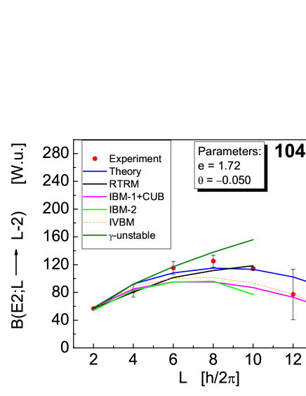
Figure 1: (Color online) Comparison of theoretical and experimental values for the $B(E2)$ transition probabilities in ${}^{104}Ru$. The theoretical results of IBM-1 with a cubic term included, IBM-2, Rigid Triaxial Rotor Model, and $\gamma$-unstable model of Wilets and Jean are also shown.

Next, we present the theoretical results for some nuclei from the $A\sim 190$ mass region. The Pt-Os region is traditionally considered within the IBM-1 framework to be a good example for the transition between $SU(3)$ and $O(6)$ IBM-OsPt . A number of theoretical calculations Bonche , CCQH , Robledo , Nomura1 , Nomura2 predict a tiny region of triaxiality between the prolate and oblate shapes in this mass region. Recent self-consistent Hartree-Fock-Bogoliubov calculations Robledo with Gogny D1S and Skyrme SLy4 forces predict that the prolate to oblate transition takes place at neutron number $N=116$ (¹⁹²Os, ¹⁹⁴Pt).

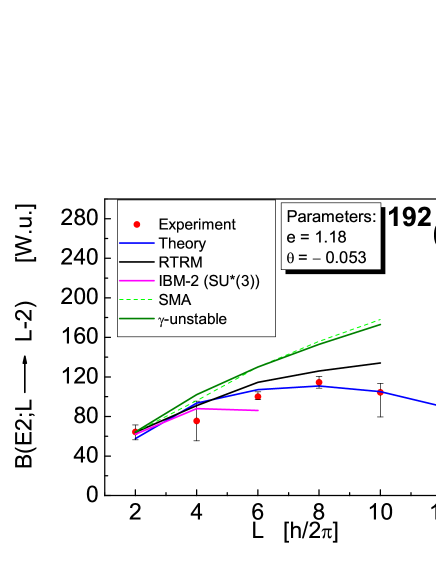
Figure 2: (Color online) Comparison of theoretical and experimental values for the $B(E2)$ transition probabilities in ${}^{192}Os$. The theoretical results of the Rigid Triaxial Rotor Model, IBM-2 in its $SU^{\ast}(3)$ limit, sextic and Mathieu approach (SMA), and $\gamma$-unstable model are also shown.

In Figure 2, the experimental $B(E2)$ values for transitions between the members of the GSB in ${}^{192}Os$ are compared with the theoretical results of IVBM, IBM-2 Walet ($SU^{\ast}(3)$ limit), RTRM Toki , sextic and Mathieu approach (SMA) Raduta , and $\gamma$-unstable model of Wilets and Jean WJ . One can see a slight reduction of the collectivity with the increasing spin well described by the IVBM, whereas the RTRM, SMA, and $\gamma$-unstable model of Wilets and Jean overestimate the observed experimental data.

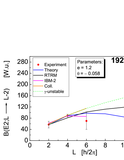
Figure 3: (Color online) Comparison of theoretical and experimental values for the $B(E2)$ transition probabilities in ${}^{192}Pt$. The theoretical results of the Rigid Triaxial Rotor Model, IBM-2, Quadrupole Collective Model, and $\gamma$-unstable model are also shown.

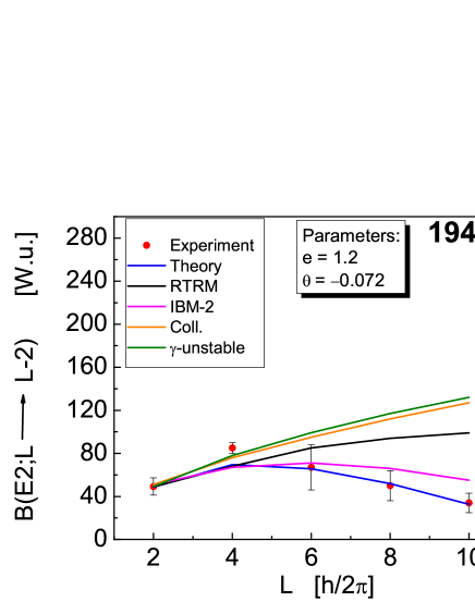
Figure 4: (Color online) Comparison of theoretical and experimental values for the $B(E2)$ transition probabilities in ${}^{194}Pt$. The theoretical results of the Rigid Triaxial Rotor Model, IBM-2, Quadrupole Collective Model, and $\gamma$-unstable model are also shown.

Next, the experimental $B(E2)$ values Nomura2 between the states of the GSB in ${}^{192}Pt$ and ${}^{194}Pt$ isotopes are shown in Figures 3 and 4, respectively, compared with the theoretical predictions of IVBM from one side, and those of IBM-2 Nomura2 , RTRM Toki , the Quadrupole Collective Model (Coll.) Nomura2 , and $\gamma$-unstable model WJ from another. The reduction in the $B(E2)$ values with increasing spin is well described by the IVBM in the two nuclei, compared to the predictions of other collective models.

From Figs. 1$-$4 one can see that the IVBM describes the $B(E2)$ transitions probabilities between the collective states of the GSB in the four considered even-even nuclei rather well. At this point we want to make some comments concerning the two parameters $e$ and $\theta$. Detailed analysis shows that the two main types of $B(E2)$ behavior - the enhancement or the reduction of the $B(E2)$ values - can be described within the present approach. The change of the values of the parameter $e$ affects mainly the scale. The coefficient in front of the second term in Eq.(43) is about of two orders of magnitude smaller than the $SU(3)$ contribution to the transition operator (43), but its role in reproducing the correct behavior of the transition probabilities between the states of the GSB is very important. At $\theta=0$ the theory gives a very specific, almost ”linear”, behavior of the $B(E2)$ values. For $\theta<0$, with the increasing of the absolute value of the parameter $\theta$ - the theoretical curve goes from that of enhanced $B(E2)$ values (which is an indication for the enhanced collectivity in the high angular momentum domain) to the case of the well-known ”cutoff effect”, which is a characteristic feature of all $SU(3)$-based calculations.

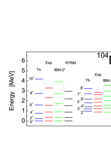
Figure 5: (Color online) Excitation energies of the GSB and $\gamma$ band in ${}^{104}Ru$, compared with the experimental data and the predictions of IBM-2 in its $SU^{\ast}(3)$ limit and RTRM. The values of the model parameters are $a_{1}=0.2155$ MeV, $b=-0.0098$ MeV, $a_{3}=-0.0002$ MeV, and $b_{3}=0.0387$ MeV.

Being a group of dynamical symmetry, the $Sp(12,R)$ through its reduction given by Eq.(6) determines the type of spectra (obtained at fixed values of the model parameters in the Hamiltonian) of different nuclei that it can describe. As an illustration, in Fig. 5 we show the theoretical results for the excitation energies of the ground and $\gamma$ bands in ${}^{104}Ru$, compared with the experimental data and the predictions Ru104e of IBM-2 in its $SU^{\ast}(3)$ limit and RTRM, both of which incorporate $\gamma$-rigid structures. The states of the $\gamma$ band are associated with the stretched states from the $\nu=-2$ irrep of $U(3,3)$. (Detailed comparison of the energy spectra obtained in the present approach for some even-even nuclei, assumed to be axially asymmetric, with experiment will be given elsewhere.) The Hamiltonian used in our calculation, expressed as a linear combination of the Casimir operators along the chain (6), is of the form

$$H=a_{1}M^{2}+b(N_{n}^{2}-N_{p}^{2})+a_{3}C_{2}[SU^{\ast}(3)]+b_{3}C_{2}[SO(3)].$$ (58)

The values of the model parameters are determined by fitting the energies of the ground and $\gamma$ bands in ${}^{104}Ru$ to the experimental data exp , using a $\chi^{2}$-procedure. From the Fig. 5 we see that the IVBM results are very similar to the ones predicted by the IBM-2. The RTRM gives better description of the collective states of the GSB, while for the $\gamma$ band it gives pronounced $\gamma$-rigid doublet structure not observed in experiment. The latter shows more regular spacings of the states in the $\gamma$ band, reasonably well reproduced by both the IVBM and IBM-2.

The results obtained for both the $B(E2)$ transition probabilities between the collective states of the GSB in the even-even nuclei under consideration and the energy levels of the GSB and $\gamma$ band in ${}^{104}Ru$ prove the correct mapping of the basis states to the experimentally observed ones. We recall the transitional character of the nucleus ${}^{104}Ru$ between $\gamma$-unstable ($O(6)$ limit) and $\gamma$-rigid ($SU^{\ast}(3)$ limit) in terms of the IBM. In this way the theoretical results obtained within the framework of IVBM suggest the range of the applicability of the present approach and reveal its relevance in the description of nuclei that exhibit axially asymmetric features in their spectra.

VII Conclusions

In the present paper we investigated the tensor properties of the algebra generators of $Sp(12,R)$ with respect to the reduction chain (6). $Sp(12,R)$ is the group of dynamical symmetry of the IVBM. The basis states of the model are also classified by the quantum numbers corresponding to the irreducible representations of the subgroups from the chain. The action of the symplectic generators as transition operators between the basis states is analyzed. The matrix elements of the $U(3,3)$ ladder operators in the so obtained symmetry-adapted basis are given.

The $U(3,3)$ limit of the symplectic IVBM is further tested on the more complicated and complex problem of reproducing the $B(E2)$ transition probabilities between the states of the ground band in some even-even nuclei from the $A=190$ and $A=190$ mass regions assumed by many authors to be axially asymmetric. In developing the theory the advantages of the algebraic approach are used for the assignment of the basis states to the experimentally observed states of the collective bands and the construction of the $E2$ transition operator as linear combination of tensor operators representing the generators of the subgroups of the respective chain. This allows the application of a specific version of the Wigner-Eckart theorem and consecutively leads to analytic results for their (reduced) matrix elements in the $U(3,3)$ symmetry-adapted basis that give the transition probabilities.

In the application to real nuclei, the parameters of the transition operator are evaluated in a fitting procedure for GSB of the considered nuclei. The $B(E2)$ transition probabilities between collective states of the ground state band in ${}^{104}Ru$, ${}^{192}Os$, ${}^{192}Pt$, and ${}^{194}Pt$ isotopes are calculated and compared with the experimental data and some other collective models that accommodate the $\gamma$-rigid or $\gamma$-soft structures. The experimental data for the presented examples are reproduced rather well, although the results are very sensitive to the values of the model parameters.

Being a group of dynamical symmetry, the $Sp(12,R)$ through its reduction given by Eq.(6) determines the type of spectra (obtained at fixed values of the model parameters in the Hamiltonian) of different nuclei that it can describe. The excited states of the GSB and $\gamma$ band in the transitional nucleus ${}^{104}Ru$ are calculated within the IVBM using a four parameter Hamiltonian, expressed as a linear combinations of the Casimir operators along the dynamical chain (6) and compared with the experimental data and the predictions of IBM-2 in its $SU^{\ast}(3)$ limit and RTRM, both of which incorporate $\gamma$-rigid structures. The structure of the two bands is reasonably well described by the present approach.

Summarizing, the results obtained for both the $B(E2)$ transitions probabilities between the collective states of the GSB in the even-even nuclei under consideration and the energy levels of the GSB and $\gamma$ band in ${}^{104}Ru$ prove the correct mapping of the basis states to the experimentally observed ones and reveal the role of the symplectic symmetries in the description of nuclei, exhibiting axially asymmetric features in their spectra.

References

(1)Dynamical Groups and Spectrum generating Algebras, Volumes 1 and 2,
edited by A. Bohm, Y. Ne’eman, and A. O. Barut (World Scientific
Publishing Co. Pte. Ltd., Singapore, 1988).
(2)Algebraic Approaches to Nuclear Structure:
Interacting Boson and Fermion Models, edited by R. F. Casten
(Harwood Academic Publishers, New York, 1993).
(3) F. Iachello, Lie Algebras and Applications, Lect.
Notes Phys. Volume 708 (Springer-Verlag, Berlin Heidelberg, 2006).
(4) Symmetries in Atomic Nuclei: From Isospin to
Supersymmetry, by A. Frank, P. V. Isacker, J. Jolie, Springer Tracks
in Modern Physics Volume 230 (Springer-Verlag, New York, 2009).
(5)Fundamentals of Nuclear Models: Foundational Models,
by D. J. Rowe, J. L. Wood (World Scientific Publisher Press,
Singapore, 2010).
(6) A. I. Georgieva, H. G. Ganev, J. P. Draayer and V. P. Garistov,
Phys. Part. Nucl. 40, 469 (2009).
(7) S. Goshen and H. J. Lipkin, Ann. Phys. (N.Y.) 6, 301
(1959); S. Goshen and H. J. Lipkin, On the Application of the Group
or to Nuclear Structure in Spectroscopic and
Group Theoretical Methods in Physics. Racah 138 Memorial Volume,
edited by F. Bloch, S. G. Goshen, A. de Shalit, S. Sambursky, and I.
Talmi (North-Holland, Amsterdam, 1968), pp. 245.
(8) G. N. Afanas’ev, E. N. Mikhailov, and P. P.
Raychev, Yad. Fiz. 14, 734 (1971); P. P. Raychev, Yad. Fiz.
16, 1171 (1972).
(9) M. Moshinsky and C. Quesne, J. Math. Phys. 12, 1772 (1971).
(10) M. Moshinsky, J. Math. Phys. 25, 1555 (1984);
E. Chacon, P. Hess, M. Moshinsky, J. Math. Phys. 25,
1565 (1984); O. Castanos, E. Chacon, and M. Moshinsky, J. Math.
Phys. 25, 1211, (1984); O. Castanos, E. Chacon, and M.
Moshinsky, J. Math. Phys. 25, 2815 (1984); M. Moshinsky, M.
Nicolesku, R. T. Sharp, J. Math. Phys. 26, 2995 (1985); E.
Chacon, P. Hess, and M. Moshinsky, J. Math. Phys. 28, 2223
(1987).
(11) G. Rosensteel and D. Rowe, Phys. Rev. Lett. 38, 10
(1977); G. Rosensteel and D. Rowe, Ann. Phys. (N.Y.) 126,
343 (1980).
(12) J. P. Draayer and G. Rosensteel, Phys. Lett. 124B,
281 (1983); J. P. Draayer and G. Rosensteel, Phys. Lett.
125B, 237 (1983); J. P. Draayer, K. J. Weeks, and G.
Rosensteel, Nucl. Phys. A413, 215 (1983).
(13) O. Castanos, P. O. Hess, J. P. Draayer, and P. Rochford, Nucl. Phys. A524,
469 (1994); D. Troltenier, J. P. Draayer, P. O. Hess, and O.
Castanos, Nucl. Phys. A576, 351 (1994).
(14) P. Kramer, Ann. Phys. (N.Y.) 141,
254, 269 (1982).
(15) V. V. Vanagas, Algebraic Foundations of
Microscopic Nuclear Theory (Nauka, Moscow, 1988) (in Russian).
(16) H. Ganev, V. P. Garistov, A.I. Georgieva, Phys. Rev.
C 69, 014305 (2004).
(17) H. G. Ganev, Phys. Rev. C83, 034307 (2011).
(18) L. Wilets and M. Jean, Phys. Rev. 102, 788 (1956).
(19) A. S. Davydov and G. F. Filippov, Nucl. Phys. 8, 237
(1958).
(20) A. E. L. Dieperink, Nucl. Phys. A421, 189c
(1984).
(21) V. Bargmann and M. Moshynsky, Nucl. Phys. 18,
697 (1960); V. Bargmann and M. Moshynsky, Nucl. Phys. 23,
177 (1961).
(22) G. Racah, Phys. Rev. 76, 1352 (1949).
(23) J. P. Elliott, Proc. R. Soc. (London), Ser.A,
245, pp. 128, 526 (1958).
(24) A. Georgieva, M. Ivanov, P. Raychev and R. Roussev, Int. J.
Theor. Phys. 25, 1181 (1986).
(25) J. Flores, J. Math. Phys. 8, 454 (1967);
J. Flores and M. Moshinsky, Nucl. Phys. A93, 81 (1967).
(26) D. J. Millenar, J. Math. Phys. 19, 1513
(1978); J. Escher and J. P. Draayer, J. Math. Phys. 39,
5123 (1998).
(27) R. Le Blanc and D. J. Rowe, J. Phys. A: Math.
Gen. 20, L681 (1987).
(28) J. P. Draayer and Y. Akiyama, J. Math. Phys.
14, 1904 (1973); Y. Akiyama and J. P. Draayer, Comput.
Phys. Commun. 5, 405 (1973).
(29) D. J. Rowe, Prog. Part. Nucl. Phys. 37, 4711
(1985).
(30) B. G. Wybourne, Classical Groups for Physicists,
(Wiley, New York, 1974); C. Quesne, J. Phys. A: Math. Gen.
23, 847 (1990); 24, 2697 (1991).
(31) G. Rosensteel and D. J. Rowe, Ann. Phys. 126, 343 (1980).
(32) A. E. L. Dieperink and R. Bijker, Phys. Lett. B116,
77 (1982).
(33) A. Frank, P. Van Isacker, and P. D. Warner,
Phys. Lett. B197, 474 (1987).
(34) D. Troltenier et al.,
Z. Phys. A 338, 261 (1991).
(35) K. Heyde, P. Van Isacker, M. Waroquier, and J.
Moreau, Phys. Rev. C 29, 1420 (1984).
(36) A. Giannatiempo, A. Nannini, P. Sona, and D. Cutoiu,
Phys. Rev. C52, 2969 (1995).
(37) H. Toki and A. Faessler,
Z. Phys. A 276, 35 (1976).
(38) R. F. Casten, and J. Cizewski,
Nucl. Phys. A309, 477 (1978).
(39) P. Bonche et al.,
Nucl. Phys. A500, 308 (1989).
(40) L. Fortunato, C. E. Alonso, J. M. Arias, J. E.
Garcia-Ramos, and A. Vitturi, Phys. Rev. C 84, 014326
(2011).
(41) L. M. Robledo, R. Rodriguez-Guzman, and P.
Sarriguren, J. Phys. G: Nucl. Part. Phys. 36, 115104
(2009).
(42) K. Nomura et al.,
Phys. Rev. C 83, 014309 (2011).
(43) K. Nomura et al.,
Phys. Rev. C 84, 014302 (2011).
(44) N. R. Walet and P. J. Brussaard,
Nucl. Phys. A474, 61 (1987).
(45) A. A. Raduta and P. Buganu, Phys. Rev.
C 83, 034313 (2011).
(46) J. Stachel at al., Nucl. Phys. A383, 429 (1982).
(47) Evaluated Nuclear Structure Data File (ENSDF),
http://ie.lbl.gov/databases/ensdfserve.html