Analysis of Aggregated Functional Data from Mixed Populations with Application to Energy Consumption

Abstract

Understanding the energy consumption patterns of different types of consumers is essential in any planning of energy distribution. However, obtaining consumption information for single individuals is often either not possible or too expensive. Therefore, we consider data from aggregations of energy use, that is, from sums of individuals’ energy use, where each individual falls into one of $C$ consumer classes. Unfortunately, the exact number of individuals of each class may be unknown: consumers do not always report the appropriate class, due to various factors including differential energy rates for different consumer classes. We develop a methodology to estimate the expected energy use of each class as a function of time and the true number of consumers in each class. We also provide some measure of uncertainty of the resulting estimates. To accomplish this, we assume that the expected consumption is a function of time that can be well approximated by a linear combination of B-splines. Individual consumer perturbations from this baseline are modeled as B-splines with random coefficients. We treat the reported numbers of consumers in each category as random variables with distribution depending on the true number of consumers in each class and on the probabilities of a consumer in one class reporting as another class. We obtain maximum likelihood estimates of all parameters via a maximization algorithm. We introduce a special numerical trick for calculating the maximum likelihood estimates of the true number of consumers in each class. We apply our method to a data set and study our method via simulation.

, , , and

t1Research supported by CAPES and ELAP/Canadian Bureau for International Education t2Research supported by CNPq grants 302755/2010-1, 476764/2010-6 and 302182/2010-1 t3Research supported by the National Science and Engineering Research Council of Canada.

1 Introduction

Efficient distribution of energy is a problem of vital importance to electric companies around the world. An important goal in energy distribution is to not overload the energy distribution system. To prevent overload, distribution networks typically have been designed to handle the maximum demand. An alternative and more efficient strategy to not only reduce the chance of overload but also to maximize the use of existing equipment is to redistribute energy to consumers so that demand is fairly constant over time. Understanding the typical energy use pattern of each type of consumer is essential for this plan.

In most regions, each energy consumer belongs to one of several classes, such as residential, commercial or industrial, and each consumer class has a different pattern of energy consumption. For example, in Brazil, residential consumers appear to have a spike in electricity consumption from 6 pm to 8 pm, due partially to the use of electric showers after the workday. Commercial and industrial consumers appear to have high electricity consumption between 8 am and 6 pm.

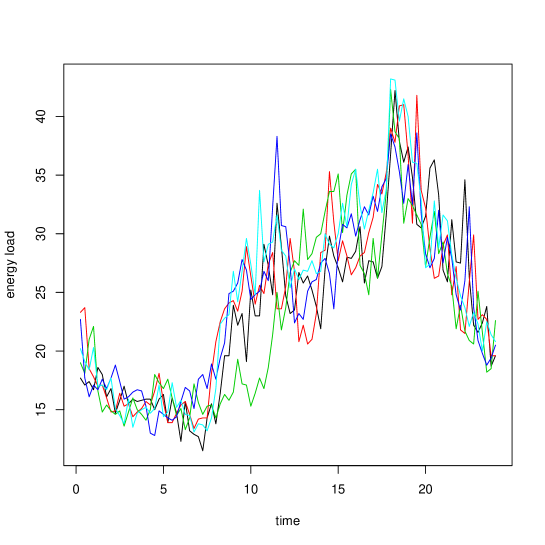
Figure 1: Data analysis: data from Transformer 1. The plot shows total electricity usage for each of five weekdays between 06/21/2002 and 06/27/2002. Each color corresponds to a different day.

One way to determine consumer energy use patterns is to monitor the energy use of each consumer in a large sample composed of different types of consumers. However, obtaining consumer-level data is costly. Furthermore, consumer-level data is extremely variable. On the other hand, aggregated data are readily available from subregions, specifically from transformers that decrease voltage and redistribute energy to consumers. Samples of daily electric load of transformers constitute our data set. Figure 1 shows the data collected from a transformer which redistributes energy to 41 consumers, with measurements recorded every fifteen minutes. The plot gives five total energy consumption curves in units of kilo-volt-amperes of the 41 consumers, one for each weekday in the period June 21 to June 27, 2002, inclusive. We see that the energy consumption curves follow a clear pattern, with little variability from day to day. For the data presented in Figure 1, we know that 7 consumers report that they are commercial consumers and 34 report that they are residential consumers. Residential consumers are of two types: those who receive monophasic electrical power and those who receive biphasic electrical power. Of the 34 residential consumers, 5 reported being monophasic and 29 reported being biphasic. However, these counts may not be accurate – consumers do not always report the appropriate class, due to various factors including differential energy rates for different consumer classes.

Our data set is from Companhia Paulista de Força e Luz (CPFL) Energia, a company that distributes electric energy in Southeast Brazil. We analyze data as in Figure 1, but from three transformers. The three transformers serve a total of 168 consumers, of whom 155 reported being residential customers and 13 reported being commercial customers. See Table 1, which contains reported counts and our estimates of true counts of consumer types.

Our goal is to use this aggregated energy use data set along with the reported number of consumers in each class to estimate the true number of consumers in each class and to estimate each class’s expected energy consumption as a function of time. Our proposed framework is to assume that each expected consumption pattern is a smooth curve that can be well approximated by a function which is a linear combination of B-splines. Individual consumer perturbations from this baseline are modeled as B-splines with random coefficients. We treat the reported numbers of consumers in each category as random variables with distribution depending on the true numbers of consumers in each class and on the probabilities of a consumer in one class reporting as another class. We obtain maximum likelihood estimates of all parameters and introduce a special numerical trick for calculating the maximum likelihood estimates of the true number of consumers in each class (see Theorem 1).

Details of our model are in Section 2, with estimates described in Section 3. In Section 4 we give details of implementation as well as extend our model and estimation procedure to the case where there are replicate observations from each transformer. Section 5 contains the analysis of the energy consumption data for the three transformers. Section 6 contains the results of a simulation study.

The estimation of typical load curves of electrical consumption using aggregated functional data was first done by Dias, Garcia and Martarelli (2009) and revisited in the Bayesian framework by Dias, Garcia and Schmidt (2013). However, these authors assumed that consumers reported their true classes.

In summary, we develop and study statistical methodology for the analysis of curve data, where the distribution of each curve depends on a class membership variable. We do not observe data from individual curves, but only observe pointwise sums. Moreover, we do not know the exact counts for class membership, only approximate counts. Our goal is to use the approximate counts and the aggregated curve data to estimate the true number of individuals in each class and to estimate the typical curve of each class. In addition, we estimate variance and covariance parameters.

In the signal processing literature the problem of aggregated information is known as linear Blind Signal Separation (BSS). The simplest model assumes the existence of $C$ independent signals $W_{1}(\cdot),\ldots,W_{C}(\cdot)$ and the observation of at least $I$ mixtures $Y_{1}(\cdot),\ldots,Y_{I}(\cdot)$, these mixtures being $Y_{i}(\cdot)=\sum_{c=1}^{C}a_{ic}W_{c}(\cdot)$, for $i=1,\ldots,I$ with unknown coefficients $a_{i1},\ldots,a_{iC}$. However, the BSS problem lies in the identification of the signals $W_{1}(\cdot),\ldots,W_{C}(\cdot)$ using only the observed data whereas in this paper we are interested in the mean and covariance functions of such processes. Usually the BSS methods are based on multivariate techniques (component analysis, orthogonalization, spatio-temporal decorrelation) which consider the time as a discrete set and do not take into account that the sources and the observations are continuous curves. For a review on the algorithms and the statistical principles of BSS see e.g. Cardoso (1998), Choi et al. (2005), and Comon and Jutten (2010).

2 Notation and model

We index transformer by $i=1,\ldots,I$, class by $c=1,\ldots,C$ and consumer served by transformer $i$ by $l=1,\ldots,N_{i}$. We denote the true class of individual $l$ served by transformer $i$ as $c_{li}$ and the reported class as $r_{li}$. We let $W_{li}(t)$ equal the electricity consumption at time $t$ of individual $l$ served by transformer $i$. We model $W_{li}$ as a hidden, random process whose distribution depends on the value of $c_{li}$. In transformer $i$, we do not observe the $W_{li}$’s but rather their sum plus measurement error, at $n_{i}$ time points, $t_{i1}<t_{i2}<\cdots<t_{in_{i}}$. For simplicity of notation and exposition, we only consider the case with $n_{i}\equiv n$ and $t_{ij}\equiv t_{j}$, for all $i$ and for $j=1,\ldots,n$. We do not observe $M_{ci}$, the true number of consumers in class $c$ served by transformer $i$. Rather, we observe $R_{ci}$, the number of reported consumers in class $c$ served by transformer $i$. Throughout, we assume that random quantities are independent from transformer to transformer.

We are interested in estimating the true counts of consumers in each class, served by each transformer, and the typical usage curve of a consumer of class $c$, which is simply the expected value of $W_{li}(t)$ when $c_{li}=c$.

2.1 Model for $W_{li}$ and the observed aggregated electricity consumption

We suppose that, for an individual of class $c$, the energy consumption is a stochastic process with distribution depending on $c$ but not on the transformer. Specifically, we suppose that $W_{li}$, the energy consumption of consumer $l$ served by transformer $i$ of consumer type $c_{li}=c$, is given by

$$W_{li}(t)\bigg{|}_{c_{li}=c}=~{}~{}\alpha_{c}(t)+\alpha_{cli}^{*}(t)$$

where $\alpha_{c}$ is the non-random typical usage curve (also called the typology) in class $c$ and $\alpha_{cli}^{*}$ is the consumer-specific random perturbation. Using the notation that the $k$th component of a vector ${v}$ is $\mbox{\boldmath${v}$}[k]$, we model $\alpha_{c}$ and $\alpha_{cli}^{*}$ with B-splines basis functions $\phi_{1},\ldots,\phi_{K}$ and $\psi_{1},\ldots,\psi_{K^{*}}$. Letting $\mbox{\boldmath{$\gamma$}}(t)=(\gamma_{1}(t),\ldots,\gamma_{K}(t))^{\prime}$ and $\mbox{\boldmath{$\psi$}}(t)$ defined similarly,

$$\alpha_{c}(t)=\sum_{k=1}^{K}\mbox{\boldmath{$\gamma$}}^{c}[k]\phi_{k}(t)\equiv\mbox{\boldmath{$\phi$}}(t)^{\prime}\mbox{\boldmath{$\gamma$}}^{c}$$ (1)

and

$$\alpha_{cli}^{*}(t)=\sum_{k=1}^{K^{*}}\mbox{\boldmath{$\gamma$}}^{cli}[k]\psi_{k}(t)\equiv\mbox{\boldmath{$\psi$}}(t)^{\prime}\mbox{\boldmath{$\gamma$}}^{cli}.$$ (2)

We suppose that the vector $\mbox{\boldmath{$\gamma$}}^{c}$ is an unknown parameter vector and the vectors $\mbox{\boldmath{$\gamma$}}^{cli}$ are random effects, normally distributed, independent with mean 0 and covariance matrix $\Sigma_{c}$. Note that this implies that, given $c_{li}=c$, $W_{li}$ is a Gaussian process with mean $\alpha_{c}$ and covariance function

$$\sigma_{c}(s,t)\equiv{\rm{cov}}(W_{li}(s),W_{li}(t))={\rm{cov}}(\alpha_{cli}^{*}(s),\alpha_{cli}^{*}(t))=\mbox{\boldmath{$\psi$}}(s)^{\prime}~{}\Sigma_{c}~{}\mbox{\boldmath{$\psi$}}(t).$$

The process $\alpha_{cli}^{*}$ allows us to account for within consumer correlation over time. We assume that the $\alpha_{cli}^{*}$’s are independent processes.

Notice that the vectors of basis function evaluations $\mbox{\boldmath{$\phi$}}(t)$ and $\mbox{\boldmath{$\psi$}}(t)$ in (1) and (2), respectively, do not depend on the consumer type $c$ – that is, we use the same size of basis ($K$ and $K^{*}$) and the same knot locations for all types of consumers. One could consider a different number of basis functions and different knot locations for each consumer class. For instance, one could place more knots around 6-9pm for residential consumers as they show a spike in electricity consumption during this time of the day. We also use the same basis functions for each transformer, that is $\mbox{\boldmath{$\phi$}}(t)$ and $\mbox{\boldmath{$\psi$}}(t)$ in (1) and (2), respectively, do not depend on $i$.

It is important to note that, in our model, $\alpha_{c}$ cannot depend on the transformer $i$, that is, that the $\mbox{\boldmath{$\gamma$}}^{c}$’s in (1) can not depend on $i$. If the $\mbox{\boldmath{$\gamma$}}^{c}$’s were to depend on $i$, we would be unable to estimate them from our data: our data consist of just one total energy curve per transformer, a curve that is a weighted sum of the unknown class-level total energy curves. By using the same $\mbox{\boldmath{$\gamma$}}^{c}$’s for all transformers, we are able to pool information across all of the transformers’ total energy curves in order to estimate the $\mbox{\boldmath{$\gamma$}}^{c}$’s.

Choosing the number of basis functions $K$, which is equivalent to choosing the number of knots, has been a subject of great research interest. Several authors suggested algorithms in order to provide a good choice of the dimension of the approximant space as a function of the sample size; see, for example, Gu (1993), Antoniadis (1994), Bodin, Villemoes and Wahlberg (2000), Kohn, Marron and Yau (2000) and De Vore, Petrova and Temlyakov (2003). However, all of these procedures, including adaptive ones such as Kooperberg and Stone (1991), Luo and Wahba (1997) and Dias (1998), deal with a non-random choice of $K$.

For consumers served by transformer $i$, we observe the total energy use plus error. We assume that the magnitude of the variability of the error does not depend on the transformer. That is, we observe the data vector ${\bf{Y}}_{i}\equiv(Y_{i}(t_{i1}),\ldots,Y_{i}(t_{in}))^{\prime}$ where, for $\epsilon_{i}(\cdot)$ and $W_{li}(\cdot)$ independent, with $\epsilon_{i}$ Gaussian white noise with var($\epsilon_{i}(t))=\sigma^{2}$,

$$Y_{i}(t) = \sum_{l=1}^{N_{i}}\sum_{c=1}^{C}W_{li}(t)~{}{\rm{I}}\{c_{li}=c\}~{}+~{}\epsilon_{i}(t)$$ (3)

$$= \sum_{c=1}^{C}M_{ci}~{}\alpha_{c}(t)~{}+~{}\sum_{l=1}^{N_{i}}\sum_{c=1}^{C}\alpha^{*}_{cli}(t){\rm{I}}\{c_{li}=c\}~{}+~{}\epsilon_{i}(t).$$

We easily see that E$(Y_{i}(t))=\sum_{c=1}^{C}M_{ci}~{}\alpha_{c}(t)$ and, because of the independence of the $\alpha_{cli}^{*}$’s,

$${\rm{cov}}(Y_{i}(s),Y_{i}(t))=\sum_{l=1}^{N_{i}}\sum_{c=1}^{C}{\rm{I}}\{c_{li}=c\}~{}{\rm{cov}}(\alpha_{cli}^{*}(s),\alpha_{cli}^{*}(t))~{}+~{}{\rm{cov}}(\epsilon_{i}(s),\epsilon_{i}(t)).$$

Defining the $n$ by $K$ matrices $\Phi$ and $\Psi$ as

$$\Phi[j,k]=\phi_{k}(t_{ij}){~{}~{}\rm{and~{}~{}}}\Psi[j,k]=\psi_{k}(t_{ij})$$

yields

$${\bf{Y}}_{i}\sim{\rm{N}}\left(\Phi\sum_{c=1}^{C}M_{ci}\mbox{\boldmath{$\gamma$}}^{c},\Psi\sum_{c=1}^{C}M_{ci}\Sigma_{c}\Psi^{\prime}+\sigma^{2}{\rm{I}}\right).$$ (4)

From (4), we see that, without further information about the $M_{ci}$’s, the distribution of ${\bf{Y}}_{i}$ is not identifiable - there are an infinite number of distinct $M_{ci}$’s and $\gamma^{c}$’s yielding the same distribution. However, when we observe the reported counts, the joint distribution of $\mathbf{Y}_{i}$ and $R_{1i},\dots,R_{Ci}$ is identifiable, provided we know the rates of misreporting.

Equation (3) considers the case where there is only one $W_{li}$ for each consumer and can be used to model the situation where $W_{li}$ is the power usage on a specified date or the average of usages on a sequence of dates. We can easily extend (3) to model the situation where there are $D_{i}$ replicates of the $W_{li}$’s for consumer $l$ served by transformer $i$. We use this extension in the simulation study and in the data analysis to model a consumer’s energy consumption on a sequence of five days, considering these five days as five replicates. The calculation and maximization of the likelihood for the replicate case is a straightforward modification of the iterative procedure described in Section 3.

2.2 Model for the reported counts of consumer classes

Recall that $r_{li}$ is the class reported by consumer $l$ served by transformer $i$, that $c_{li}$ is the consumer’s true class, that $M_{ci}$ is the true number of consumers of class $c$ served by transformer $i$ and that $R_{ci}$ is the corresponding reported number. We suppose that all consumers report some class, that is, that $N_{i}$, the total number of consumers served by transformer $i$, is equal to $\sum_{c}R_{ci}$, which is also equal to $\sum_{c}M_{ci}$. Recall that, in our model, the $M_{ci}$’s are fixed parameters and the $R_{ci}$’s are random variables. We require a model for consumer reporting, that is, for $R_{1i},\ldots,R_{Ci}$ for true counts $M_{1i},\ldots,M_{Ci}$.

To model consumer reporting, we suppose that there is a known fraud matrix ${\cal{F}}$, not depending on the transformer, with

$${\cal{F}}(c,r)=P\{r_{li}=r|c_{li}=c\},~{}r,c=1,\ldots,C,$$

the probability that a consumer of class $c$ reports as being of class $r$. We assume that consumers report independently of other consumers.

Table 2, a $C$ by $C$ table of counts, is useful in understanding the distribution of the reported counts. For convenience, we drop the transformer subscript $i$. Let $x_{cj}$ be the number of consumers who are of class $c$ but report they are of class $j$. The reported number of consumers of class $j$ is the sum of counts in column $j$: $R_{j}=\sum_{c}x_{cj}$. The true number of consumers of class $c$ is the sum of counts in row $c$: $M_{c}=\sum_{j}x_{cj}.$

For $c=1,\ldots,C$, let ${\bf{X}}_{c}\equiv(x_{c1},\ldots,x_{cC})^{\prime}$, the vector of reported counts from consumers of class $c$, found in row $c$ of the count table with row total equal to $M_{c}$. Then ${\bf{X}}_{c}$ is multinomial$(M_{c},{\cal{F}}(c,1),\ldots,{\cal{F}}(c,C))$. By independence of consumer reporting, ${\bf{X}}_{1},\ldots,{\bf{X}}_{C}$ are independent. Thus, we have defined the joint distribution of $R_{1}=\sum_{c}x_{c1},\ldots,R_{C}=\sum_{c}x_{cC}$ when the true class counts are $M_{1},\ldots,M_{C}$.

3 Maximum Likelihood Estimation

We estimate the parameters by maximizing the log likelihood. Let the parameter vectors describing the $W_{li}$ processes be those defining the class means, the $\alpha_{c}$’s, that is, let the set of parameter vectors describing the $W_{li}$ processes be ${\cal{G}}=(\mbox{\boldmath{$\gamma$}}^{1},\ldots,\mbox{\boldmath{$\gamma$}}^{C})^{\prime}$. Let the set of parameters defining the class variance structure be ${\cal{S}}=\{\Sigma_{1},\ldots,\Sigma_{C}\}$. Recall that $\sigma^{2}$ is the measurement error variance. Let ${\bf{M}}_{i}=(M_{1i},\ldots,M_{Ci})^{\prime}$ be the vector of true class counts in transformer $i$ and ${\bf{M}}$ the collection of true counts, ${\bf{M}}_{1},\ldots,{\bf{M}}_{I}$. Recall that the elements of ${\bf{M}}$ are unknown parameters.

The data are ${\bf{Y}}_{i}$ as in (4) and ${\bf{R}}_{i}=(R_{1i},\ldots,R_{Ci})^{\prime}$, the reported counts, for transformers $i=1,\ldots,I$.

By the independence of the transformers, the log likelihood is

$${\cal{L}}({\cal{G}},{\cal{S}},{\sigma}^{2},{\bf{M}})=\sum_{i=1}^{I}{\cal{L}}_{i}({\cal{G}},{\cal{S}},\sigma^{2},{\bf{M}}_{i})$$

where

$${\cal{L}}_{i}({\cal{G}},{\cal{S}},\sigma^{2},{\bf{M}}_{i}) \equiv {\cal{L}}_{i}({\cal{G}},{\cal{S}},\sigma^{2},{\bf{M}}_{i}\big{|}{\bf{Y}}_{i},{\bf{R}}_{i})$$ (5)

$$= \log~{}\big{[}~{}f_{Y_{i}}({\bf{Y}}_{i}\big{|}{\cal{G}},{\cal{S}},\sigma^{2},{\bf{M}}_{i})\times P\{{\bf{R}}_{i}|{\bf{M}}_{i}\}~{}\big{]}$$

where $P\{{\bf{R}}_{i}\big{|}{\bf{M}}_{i}\}$ is the probability mass function of ${\bf{R}}_{i}$ calculated assuming that the true consumer category counts for transformer $i$ are the components of the vector ${\bf{M}}_{i}$. The expression for $\log[f_{Y_{i}}({\bf{Y}}_{i}\big{|}{\cal{G}},{\cal{S}},\sigma^{2},{\bf{M}}_{i})]$ follows directly from our model (4). The other part of ${\cal{L}}_{i}$, $P\{{\bf{R}}_{i}\big{|}{\bf{M}}_{i}\}$, is discussed in Sections 3.3 and 3.4.

3.1 Maximization procedure

We carry out the maximization of ${\cal{L}}$ iteratively and step-wise, where, at the $s$th iteration, we update the parameter estimates ${\cal{G}}^{(s)}$, ${\cal{S}}^{(s)}$, ${\sigma}^{2(s)}$ and ${\bf{M}}^{(s)}$ to ${\cal{G}}^{(s+1)}$, ${\cal{S}}^{(s+1)}$, ${\sigma}^{2(s+1)}$ and ${\bf{M}}^{(s+1)}$ so that ${\cal{L}}({\cal{G}}^{(s+1)},{\cal{S}}^{(s+1)},{\sigma}^{2(s+1)},{\bf{M}}^{(s+1)})$ $\geq{\cal{L}}({\cal{G}}^{(s)},{\cal{S}}^{(s)},{\sigma}^{2(s)},$ ${\bf{M}}^{(s)})$. We initialize the procedure by taking ${\bf{M}}_{i}^{(0)}\equiv{\bf{R}}_{i}$. We then carry out the following two steps until convergence. Details of each step follow in Sections 3.2, 3.3 and 4.

1. Given ${\bf{M}}^{(s)}$, we let ${\cal{G}}^{(s+1)}$, ${\cal{S}}^{(s+1)}$ and ${\sigma}^{2(s+1)}$ maximize the log likelihood, or at least not decrease the log likelihood.

2. Given ${\cal{G}}^{(s+1)}$, ${\cal{S}}^{(s+1)}$ and ${\sigma}^{2(s+1)}$, we let ${\bf{M}}^{(s+1)}$ maximize the log likelihood, or at least not decrease the log likelihood.

We have no theory to prove that the maximum likelihood is unique or that our iterative procedure converges. However, in all of our analyses - of simulated data and of the transformer data - our procedure always converged. To study the possible problem of multi-modality of the likelihood function, for a few data sets we used several different sets of starting values for the parameter estimates. In all cases, the algorithm converged to the same final parameter estimates.

3.2 Step 1: updating ${\cal{G}}$, ${\cal{S}}$ and ${\sigma}^{2}$

Using ${\bf{Y}}_{i}$’s normal distribution in (4), we see that we must minimize

$$l_{1}({\cal{G}},{\cal{S}},{\sigma}^{2})\equiv\sum_{i=1}^{I}\log\Big{|}\Psi\sum_{c=1}^{C}M_{ci}\Sigma_{c}\Psi^{\prime}+\sigma^{2}{\rm{I}}\Big{|}$$

$$+\sum_{i=1}^{I}\left({\bf{Y}}_{i}-\sum_{c=1}^{C}M_{ci}\Phi\mbox{\boldmath{$\gamma$}}^{c}\right)^{\prime}\left(\Psi\sum_{c=1}^{C}M_{ci}\Sigma_{c}\Psi^{\prime}+\sigma^{2}{\rm{I}}\right)^{-1}\left({\bf{Y}}_{i}-\sum_{c=1}^{C}M_{ci}\Phi\mbox{\boldmath{$\gamma$}}^{c}\ \right)$$

as a function of ${\cal{G}}$, ${\cal{S}}$ and ${\sigma}^{2}$, keeping the $M_{ci}$’s fixed. We carry this out iteratively, in three steps:

1. Given ${{\cal{S}}}^{(s)}$ and ${\sigma}^{2(s)}$, let ${\cal{G}}^{(s+1)}$ minimize $l_{1}$. This step poses no problem and can be done explicitly yielding

   $${\cal{G}}^{(s+1)} = \left(\displaystyle\sum_{i=1}^{I}\left[M_{1i}^{(s)}\Phi\cdots M_{Ci}^{(s)}\Phi\right]^{\prime}\Lambda_{i}^{-1}\left[M_{1i}^{(s)}\Phi\cdots M_{Ci}^{(s)}\Phi\right]\right)^{-1}$$ (6)

   $$\quad\times\left(\displaystyle\sum_{i=1}^{I}\left[M_{1i}^{(s)}\Phi\cdots M_{Ci}^{(s)}\Phi\right]^{\prime}\Lambda_{i}^{-1}\mathbf{Y}_{i}\right),$$

   where $\Lambda_{i}=\left(\Psi\sum_{c=1}^{C}M_{ci}^{(s)}\Sigma_{c}^{(s)}\Psi^{\prime}+\sigma^{2(s)}\mathbf{I}\right)$.

2. Given ${\cal{G}}^{(s+1)}$ and ${{\cal{S}}}^{(s)}$, find ${\sigma}^{2(s+1)}$ that minimizes $l_{1}$. This would generally require a numerical minimization.

3. Given ${\cal{G}}^{(s+1)}$ and ${\sigma}^{2(s+1)}$, let ${\cal{S}}^{(s+1)}$ minimize $l_{1}$. This is the most challenging step and will typically require simplifying assumptions of the form of the $\Sigma_{c}$’s, as in Section 4. In addition, this would generally require a numerical minimization.

3.3 Step 2: updating ${\bf{M}}_{1},\ldots,{\bf{M}}_{I}$

Note that, to maximize the log likelihood with respect to ${\bf{M}}_{1},\ldots,{\bf{M}}_{I}$, we can carry out $I$ separate maximizations, one for each transformer. That is, for each fixed $i=1,\ldots,I$, we seek $M_{ci}$, $c=1,\ldots,C$ to maximize ${\cal{L}}_{i}({\cal{G}},{\cal{S}},\sigma^{2},{\bf{M}}_{i})$ in (5), treating ${\cal{G}}$, ${\cal{S}}$, and $\sigma^{2}$ as fixed.

This step brings challenges. The function $P\{{\bf{R}}_{i}\big{|}{\bf{M}}_{i}\}$ does not have a closed form, nor does its derivative. Furthermore, Newton-Raphson type methods of maximization are inappropriate since each $M_{ci}$ is an integer with plausible values usually within a small range of the reported count $R_{ci}$. Therefore the possible values of $M_{ci}$ must be treated as integer.

We can approximate the function $P\{{\bf{R}}_{i}\big{|}{\bf{M}}_{i}\}$ via simulation. The most natural simulation is a “brute force” one: for each fixed ${\bf{M}}_{i}$ we would generate a large number of ${\bf{R}}_{i}$’s according to the model described in Section 2.2 and calculate the proportion of times the generated ${\bf{R}}_{i}$ is equal to the observed ${\bf{R}}_{i}$. For instance, consider the case that transformer $i$ serves 50 consumers, of two classes, with the reported number of residential consumers $R_{1i}=$40 and the reported number of commercial consumers $R_{2i}=$10. We would want to calculate $P\{R_{1i}=40,R_{2i}=10|M_{1i}=m_{1},M_{2i}=50-m_{1}\}$ for all values of $m_{1}$, or at least all plausible values of $m_{1}$. Thus, we would want to carry out many simulations – 51 if we wanted to consider all possible values of $m_{1}$. We would have to do this for each transformer. Clearly, a short cut would be desirable.

Fortunately, we have determined a less computer intensive simulation method to approximate $P\{{\bf{R}}_{i}\big{|}{\bf{M}}_{i}\}$, justified by Theorem 1 in the next section. We show that we can calculate $P\{{\bf{R}}_{i}\big{|}{\bf{M}}_{i}\}$ in ${\cal{L}}_{i}$ via a function $H_{i}$. We can easily and quickly approximate and table $H_{i}(m)$ for all values of $m$ with only one simulation per transformer. Thus, to maximize ${\cal{L}}_{i}$, by Theorem 1, it suffices to find ${\bf{M}}_{i}$ to maximize

$${\cal{L}}_{i}^{*}({\bf{M}}_{i}|{\bf{Y}}_{i},{\bf{R}}_{i})\equiv{\cal{L}}_{i}^{*}({\bf{M}}_{i})\equiv-\frac{1}{2}\log\Big{|}\Psi\sum_{c=1}^{C}M_{ci}\Sigma_{c}\Psi^{\prime}+\sigma^{2}{\rm{I}}\Big{|}$$

$$-\frac{1}{2}\left({\bf{Y}}_{i}-\sum_{c=1}^{C}M_{ci}\Phi\mbox{\boldmath{$\gamma$}}^{c}\right)^{\prime}\left(\Psi\sum_{c=1}^{C}M_{ci}\Sigma_{c}\Psi^{\prime}+\sigma^{2}{\rm{I}}\right)^{-1}\left({\bf{Y}}_{i}-\sum_{c=1}^{C}M_{ci}\Phi\mbox{\boldmath{$\gamma$}}^{c}\ \right)$$

$$+\sum_{c=1}^{C}\log M_{ci}!+\log H_{i}({\bf{M}}_{i}).$$

In our data analyses and simulation studies, we easily calculated ${\cal{L}}_{i}^{*}({\bf{M}}_{i})$ for all possible values of ${\bf{M}}_{i}$ and chose the value of ${\bf{M}}_{i}$ that maximized ${\cal{L}}_{i}^{*}$. If this is not practical, then one could calculate ${\cal{L}}_{i}^{*}$ for a small range of values of ${\bf{M}}_{i}$.

3.4 Alternate form for P$({\bf{R}}_{i}|{\bf{M}}_{i})$

For convenience, we will once again drop $i$, the subscript indicating the transformer. Recall the notation and the definitions in Section 2.2, where we defined the joint distribution of $R_{1},\ldots,R_{C}$ by defining the distribution of the rows of Table 2. Here, we derive an expression for the probability that $R_{1}=\mathpzc{r}_{1},\ldots,R_{C}=\mathpzc{r}_{C}$ in terms of random vectors, $\tilde{{\bf{X}}}_{1},\ldots,\tilde{{\bf{X}}}_{C}$, that resemble the columns of Table 2. Specifically, for $j=1,\ldots,C$, let $\tilde{{\bf{X}}}_{j}$ be multinomial with parameters $\mathpzc{r}_{j},p_{1j},p_{2j},\ldots,$ and $p_{Cj}$ with

$$p_{cj}=\frac{{\cal{F}}(c,j)}{\sum_{l=1}^{C}{\cal{F}}(l,j)}.$$ (7)

Thus, the entries of each $\tilde{{\bf{X}}}_{j}$ sum to $\mathpzc{r}_{j}$ and the multinomial probability associated with the $c$th component of $\tilde{{\bf{X}}}_{j}$ is proportional to ${\cal{F}}(c,j)$, the probability that a consumer of class $c$ reports being in class $j$. That is, $\tilde{{\bf{X}}}_{j}$ is a vector of counts, dividing up the $\mathpzc{r}_{j}$ consumers who have reported being class $j$ into their true classes. While the distribution of $\tilde{{\bf{X}}}_{j}$ is not equal to the conditional distribution of column $j$ of Table 2 given $R_{j}=\mathpzc{r}_{j}$, the distribution of $\tilde{{\bf{X}}}_{j}$ does relate to the distribution of $R_{1},\ldots,R_{C}$, as given in the following theorem.

Theorem 1.

For the random variables $R_{1},\ldots,R_{C}$ as defined in Section 2.2 and for $\tilde{{\bf{X}}}_{1},\ldots,\tilde{{\bf{X}}}_{C}$ independent with distributions as defined above,

$$P\{{\bf{R}}={\bf{r}}|{\bf{M}}={\bf{m}}\} = P\{R_{1}=\mathpzc{r}_{1},\ldots,R_{C}=\mathpzc{r}_{C}|M_{1}=m_{1}\ldots,M_{C}=m_{C}\}$$

$$= \frac{\prod_{j=1}^{C}\left[\sum_{c=1}^{C}{\cal{F}}(c,j)\right]^{r_{j}}}{\prod_{j=1}^{C}\mathpzc{r}_{j}!}\times\prod_{c=1}^{C}m_{c}!\times H(m_{1},\ldots,m_{C})$$

where

$$H(m_{1},\ldots,m_{C})={\rm{E}}\left({\rm{I}}\bigg{\{}\sum_{j=1}^{C}\tilde{{\bf{X}}}_{j}[c]=m_{c},c=1,\ldots,C\bigg{\}}\right).$$ (8)

Comment. Theorem 1 allows us to approximate $P\{{\bf{R}}={\bf{r}}|{\bf{M}}={\bf{m}}\}$ for fixed ${\bf{r}}$ via one simulation study. To understand this, consider the following simple example. Suppose there are two classes and we have data from a transformer that serves 75 clients, with reported counts $\mathpzc{r}_{1}=32$ and $\mathpzc{r}_{2}=43$. Suppose that the fraud matrix is

$${\cal{F}}=\left[\begin{array}[]{ccc}0.98&0.02\\ 0.05&0.95\end{array}\right].$$ (9)

The “brute force” way to approximate $P\{R_{1}=32,R_{2}=43|M_{1}=m_{1},M_{2}=m_{2}\}$ (the way we avoid) is to carry out one simulation study for each vector $(m_{1},m_{2})$, generating vectors ${\bf{X}}_{1},{\bf{X}}_{2}$ and counting the proportion of times that ${\bf{X}}_{1}+{\bf{X}}_{2}$ equals (32,43)^′. Fortunately, the Theorem gives a form for $P\{R_{1}=32,R_{2}=43|M_{1}=m_{1},M_{2}=m_{2}\}$ that allows us to carry out just one simulation study that can then be used for all vectors $(m_{1},m_{2})$, as follows. We simulate $B$ data sets, with the $b$th simulated data set consisting of two independent multinomial vectors:

$$\tilde{{\bf{X}}}_{1}^{b}~{}\sim~{}{\rm{~{}multinomial}}\left(32,\frac{0.98}{1.03},\frac{0.05}{1.03},\right),$$

and

$$\tilde{{\bf{X}}}_{2}^{b}~{}\sim~{}{\rm{~{}multinomial}}\left(43,\frac{0.02}{0.97},\frac{0.95}{0.97}\right).$$

Let $M_{1}^{b}$ and $M_{2}^{b}$ correspond to the row totals: $M_{c}^{b}=\tilde{{\bf{X}}}_{1}^{b}[c]+\tilde{{\bf{X}}}_{2}^{b}[c]$. We then approximate ${H}$ via $\hat{H}$, using the $M_{1}^{b}$’s and $M_{2}^{b}$’s that result from the simulation. For instance, $\hat{H}(34,42)$ is the proportion of the $B$ simulated data sets that had $M_{1}^{b}=34$ and $M_{2}^{b}=42$.

We carry out this procedure with $B=100,000$ runs. Table 3 shows the resulting approximations of $H(m_{1},75-m_{1})$ when $R_{1}=32$ and $R_{2}=43$.

In general, to estimate $H$, we simulate $B$ independent sets distributed as $\{\tilde{{\bf{X}}}_{1},\ldots,\tilde{{\bf{X}}}_{C}\}$, with the $b$th simulated data set denoted $\{\tilde{{\bf{X}}}_{1b},\ldots,\tilde{{\bf{X}}}_{Cb}\}$, $b=1,\ldots,B$. We let

$$\hat{H}(m_{1},\ldots,m_{C})=\frac{1}{B}\sum_{b=1}^{B}{\rm{I}}\bigg{\{}\sum_{j=1}^{C}\tilde{{\bf{X}}}_{jb}[c]=m_{c},c=1,\ldots,C\bigg{\}}.$$

Proof of Theorem 1. Write $P\{{\bf{R}}={\bf{r}}|{\bf{M}}={\bf{m}}\}$ as

$$\sum_{x_{cj}:\sum_{c}x_{cj}=\mathpzc{r}_{j}}P\{{\bf{X}}_{1}=(x_{11},\ldots,x_{1C})\}~{}\times$$

$$\times~{}P\{{\bf{X}}_{2}=(x_{21},\ldots,x_{2C})\}\times\cdots\times P\{{\bf{X}}_{C}=(x_{C1},\ldots,x_{CC})\}$$

$$=\sum_{\begin{subarray}{c}x_{cj}:\sum_{c}x_{cj}=\mathpzc{r}_{j}\\ {\rm{and}}~{}\sum_{j}x_{cj}=m_{c}\end{subarray}}\Bigg{\{}\left[\frac{m_{1}!}{x_{11}!\cdots x_{1C}!}{\cal{F}}(1,1)^{x_{11}}\cdots{\cal{F}}(1,C)^{x_{1C}}\right]\times\cdots$$

$$\times\left[\frac{m_{C}!}{x_{C1}!\cdots x_{CC}!}{\cal{F}}(C,1)^{x_{C1}}\cdots{\cal{F}}(C,C)^{x_{CC}}\right]\Bigg{\}}.$$

Rearranging terms yields that the probability is equal to

$$\frac{\prod_{c=1}^{C}m_{c}!}{\prod_{c=1}^{C}\mathpzc{r}_{c}!}~{}\sum_{\begin{subarray}{c}x_{cj}:\sum_{c}x_{cj}=\mathpzc{r}_{j}\\ {\rm{and}}~{}\sum_{j}x_{cj}=m_{c}\end{subarray}}\Bigg{\{}\left[\frac{\mathpzc{r}_{1}!}{x_{11}!x_{21}!\cdots x_{C1}!}{\cal{F}}(1,1)^{x_{11}}\cdots{\cal{F}}(C,1)^{x_{C1}}\right]\times\cdots$$

$$\times\left[\frac{\mathpzc{r}_{C}!}{x_{1C}!x_{2C}!\cdots x_{CC}!}{\cal{F}}(1,C)^{x_{1C}}\cdots{\cal{F}}(C,C)^{x_{CC}}\right]\Bigg{\}}$$

$$= \frac{\prod_{c=1}^{C}m_{c}!}{\prod_{c=1}^{C}\mathpzc{r}_{c}!}~{}\sum_{\begin{subarray}{c}x_{cj}:\sum_{c}x_{cj}=\mathpzc{r}_{j}\\ {\rm{and}}~{}\sum_{j}x_{cj}=m_{c}\end{subarray}}\left[\frac{\mathpzc{r}_{1}!}{x_{11}!x_{21}!\cdots x_{C1}!}p_{11}^{x_{11}}p_{21}^{x_{21}}\cdots p_{C1}^{x_{C1}}\right]\times\cdots$$

$$\times\left[\frac{\mathpzc{r}_{C}!}{x_{1C}!x_{2C}!\cdots x_{CC}!}p_{1C}^{x_{1C}}p_{2C}^{x_{2C}}\cdots p_{CC}^{x_{CC}}\right]~{}~{}\times\prod_{j=1}^{C}\left[\sum_{c=1}^{C}{\cal{F}}(c,j)\right]^{\mathpzc{r}_{j}}$$

$$= \frac{\prod_{j=1}^{C}\left[\sum_{c=1}^{C}{\cal{F}}(c,j)\right]^{\mathpzc{r}_{j}}}{\prod_{c=1}^{C}\mathpzc{r}_{c}!}\times\prod_{c=1}^{C}m_{c}!\times$$

$$~{}~{}\times\sum_{x_{cj}:\sum_{j}x_{cj}=m_{c}}{\prod_{j=1}^{C}}P\{\tilde{{\bf{X}}}_{j}=(x_{1j},\ldots,x_{Cj})\}$$

$$= \frac{\prod_{j=1}^{C}\left[\sum_{c=1}^{C}{\cal{F}}(c,j)\right]^{\mathpzc{r}_{j}}}{\prod_{c=1}^{C}\mathpzc{r}_{c}!}\times\prod_{c=1}^{C}m_{c}!\times H(m_{1},\ldots,m_{C}).$$

4 Details of Implementation

We now give details of implementation concerning choice of starting values of the parameter estimates, maximization of the likelihood under the restriction that $\Sigma_{c}=\sigma^{2}_{\gamma,c}{\rm{I}}$ and the choice of software.

As previously mentioned, we recommend using the reported counts as the initial estimates of the true counts.

Recall from Section 2.1 that we assume the magnitude of the variability of the error does not depend on the transformer, that is, $\sigma^{2}_{i}=\sigma^{2}$ for all $i=1,\ldots,I$. To obtain the initial estimate of $\sigma^{2}$ in the replicate case, we first fit a smoothing spline curve to each replicate in transformer $i$ and calculate the sample variance of the residuals of that fit adjusting for the correct degrees of freedom, which are based on the trace of the smoothing hat matrix. We then pool those variances across replicates and transformers to obtain our initial estimate of $\sigma^{2}$. For the non-replicate case the procedure is the same, but we only need to pool across transformers. More details on smoothing based estimation of variances and calculation of appropriate degrees of freedom can be found in Wahba (1983).

Since we assume that the $\mbox{\boldmath{$\gamma$}}^{cli}$’s have covariance $\Sigma_{c}=\sigma_{\gamma,c}^{2}{\rm{I}}$, the set of covariance parameters ${\cal{S}}$ is equal to $\{\sigma_{\gamma,c}^{2},c=1,\ldots,C\}$. We use method of moments for our initial estimates of the $\sigma_{\gamma,c}^{2}$’s, using the fact that ${\bf{Y}}_{i}$ has a multivariate distribution with covariance matrix $[\sum_{c=1}^{C}M_{ci}\sigma_{\gamma,c}^{2}]\Psi\Psi^{\prime}+\sigma^{2}{\rm{I}}]$. For the purpose of calculating the initial estimates, we suppose that prior knowledge tells us that $\sigma_{\gamma,c}^{2}=s_{c}\sigma_{\gamma,C}^{2}$ for some known $s_{c}$’s, $c=1,\ldots,C-1$. To extend this notation, we set $s_{C}=1$.

In the non-replicate case, we write

$$\sum_{i,j}{\rm{var}}({\bf{Y}}_{i}[j])=\sigma_{\gamma,C}^{2}\sum_{i}\left[\sum_{c=1}^{C}M_{ci}s_{c}\right]{\rm{trace}}(\Psi\Psi^{\prime})+In\sigma^{2}.$$ (10)

We use our initial estimates of $M_{ci}$ and $\mbox{\boldmath{$\gamma$}}^{c}$ to form the estimate of the left side of (10):

$$\sum_{j}\widehat{{\rm{var}}}({\bf{Y}}_{i}[j])=||{\bf{Y}}_{i}-\widehat{M}_{ci}^{(0)}\Phi\hat{\mbox{\boldmath{$\gamma$}}}^{c(0)}||^{2}.$$

We substitute our estimates of the $M_{ci}$’s and the $\sigma^{2}$’s into the right side of (10) and then solve for our estimate of $\sigma_{\gamma,C}^{2}$. This yields our initial estimate, $\hat{\sigma}_{\gamma,C}^{2(0)}$, and our other initial estimates, $\hat{\sigma}_{\gamma,c}^{2(0)}\equiv s_{c}\hat{\sigma}_{\gamma,C}^{2(0)}$.

In the case where we observe $D$ replicates from transformer $i$, we modify the calculations, summing both sides of (10):

$$\sum_{d,i,j}{\rm{var}}({\bf{Y}}_{i,d}[j])=D\Bigg{\{}\sigma_{\gamma,C}^{2}\sum_{i}\left[\sum_{c=1}^{C}M_{ci}s_{c}\right]{\rm{trace}}(\Psi\Psi^{\prime})+In\sigma^{2}\Bigg{\}}$$

and estimating the variance of ${\bf{Y}}_{i,d}[j]$ by the sample variance of ${\bf{Y}}_{i,1}[j]$, $\ldots,{\bf{Y}}_{i,D}[j]$.

To maximize the likelihood, we carry out Steps 1, 2 and 3 of the updating algorithm of Section 3.2. Step 1 is straightforward. For the one-dimensional maximization of Step 2, that is, for updating estimates of $\sigma^{2}$, we use the $R$ function optimize.

For Step 3 of the updating algorithm, we must minimize $l_{1}$ with respect to the $\sigma_{\gamma,c}^{2}$’s. First, write

$$\Psi\sum_{c=1}^{C}M_{ci}\Sigma_{c}\Psi^{\prime}+\sigma^{2}{\rm{I}}=\left(\sum_{c=1}^{C}M_{ci}\sigma^{2}_{\gamma,c}\right)\Psi\Psi^{\prime}+\sigma^{2}{\rm{I}}.$$

Writing the eigenvalue-eigenvector decomposition $\Psi\Psi^{\prime}$ as $Q^{\prime}\Gamma Q$ with $\Gamma$ diagonal and $Q$ orthonormal yields

$$\left[\left(\sum_{c=1}^{C}M_{ci}\sigma^{2}_{\gamma,c}\right)\Psi\Psi^{\prime}+\sigma^{2}{\rm{I}}\right]^{-1}=Q^{\prime}\left[\left(\sum_{c=1}^{C}M_{ci}\sigma^{2}_{\gamma,c}\right)\Gamma+\sigma^{2}{\rm{I}}\right]^{-1}Q.$$

Let $\Delta_{i}=\Delta_{i}(\sigma^{2}_{\gamma,1},\ldots,\sigma^{2}_{\gamma,C})$ be the diagonal matrix

$$\Delta_{i}=\left(\sum_{c=1}^{C}M_{ci}\sigma^{2}_{\gamma,c}\right)\Gamma+\sigma^{2}{\rm{I}}.$$

Thus, letting ${\bf{Y}}_{i}^{*}=Q({\bf{Y}}_{i}-\sum_{c}M_{ci}\Phi\mbox{\boldmath{$\gamma$}}^{c})$, we must find $\sigma^{2}_{\gamma,1},\ldots,\sigma^{2}_{\gamma,C}$ to minimize

$$l_{1}({\cal{G}},\{\sigma^{2}_{\gamma,1},\ldots,\sigma^{2}_{\gamma,C}\},{\sigma}^{2})=\sum_{i}\log\left|\Delta_{i}\right|+\sum_{i}{{\bf{Y}}_{i}^{*}}^{\prime}\Delta_{i}^{-1}{\bf{Y}}_{i}^{*}.$$

Since $\Delta_{i}$ is diagonal, the minimization can be easily carried out numerically via a $C$-dimensional optimization. Here, we have used the $R$ function optim with method L-BFGS-B, which is a modification of the quasi-Newton method. This function allows specification of a lower and upper bound for each variable, which we need to force variance parameter estimates to be non-negative. Note that we can calculate $Q$ and $\Gamma$ at the beginning of our iterations, as they are determined by the choice of basis. The modification of Step 3 for the replicate case is similar.

5 Data analysis

Recall that our data set consists of energy consumption data from three transformers, recorded every 15 minutes during five days of a particular week. For each transformer, we have $C=3$ consumer types, residential monophasic $(c=1)$, residential biphasic $(c=2)$ and commercial $(c=3)$. In our analysis, we use the methods of Section 4 with $D=5$ replicates, one for each weekday.

In the analysis, we consider the fraud matrix given by

$${\cal{F}}=\left[\begin{array}[]{ccc}0.96&0.02&0.02\\ 0&0.98&0.02\\ 0.05&0.05&0.9\end{array}\right],$$ (11)

where a commercial consumer self-reports as either a monophasic or biphasic residential consumer, each with probability 0.05. A residential biphasic consumer never self-reports as monophasic and self-reports as a commercial consumer with probability 0.02. A monophasic consumer self-reports as biphasic with probability 0.02 and as commercial with probability 0.02. The misreporting occurs because commercial consumers pay a higher rate for their energy than residential consumers and, therefore, small business owners may report themselves as either residential monophasic or biphasic consumers. The other type of misreporting is rare, but possible. For example, a consumer with a business and residence at the same location may close the business but fail to notify the energy company. Another example would be a residential consumer that self-reports biphasic but actually behaves as a monophasic consumer, using only 127 volts. On the other hand, a biphasic consumer cannot self-report as a monophasic consumer because the energy company knows the voltage power of the residences. All this information can be obtained from the experts in the field.

We model the energy load of transformer $i$ on day $d$ as defined in Sections 2 and 4. We use the same $\phi$’s as $\psi$’s, a set of nine cubic B-spline basis functions with equally spaced knots. We consider the case where $\Sigma_{c}$ = $\sigma^{2}_{\gamma,c}$ ${{\rm{I}}}$, $c=1,2,3$, and $\sigma_{i}^{2}=\sigma^{2}$, $i=1,\ldots,I$.

We find initial estimates of $\sigma^{2}$, $\sigma^{2}_{\gamma,1}$ , $\sigma^{2}_{\gamma,2}$ and $\sigma^{2}_{\gamma,3}$ using the methods described in Section 4. Specifically, we calculate the ${\bf\hat{Y}}_{id}$’s using cubic smoothing splines. We choose one smoothing parameter by eye, to use for all spline fits. The chosen smoothing parameter results in using 10 degrees of freedom to fit each replicate. We find $\hat{\sigma}^{2(0)}$ via

$$\hat{\sigma}^{2(0)}=\frac{\displaystyle\sum_{i=1}^{3}\sum_{d=1}^{5}\sum_{j=1}^{96}\|{\bf{Y}}_{id}[j]-{\hat{{\bf{Y}}}_{id}[j]}\|^{2}}{15(96-10)}=7.16.$$ (12)

To find our initial estimates, we suppose that $\sigma^{2}_{\gamma,2}$ = $\sigma^{2}_{\gamma,1}$ and $\sigma^{2}_{\gamma,3}$ = $\sigma_{\gamma,1}^{2}$, which yields $\hat{\sigma}^{2(0)}_{\gamma,1}=\hat{\sigma}^{2(0)}_{\gamma,2}=0.074$ and $\hat{\sigma}^{2(0)}_{\gamma,3}=0.446$. After our iterative maximization of the likelihood, we obtain our final estimates for the variance parameters: ${\hat{\sigma}^{2}}=7.17$, $\hat{\sigma}^{2}_{\gamma,1}=0.102$, $\hat{\sigma}^{2}_{\gamma,2}=0.011$ and $\hat{\sigma}^{2}_{\gamma,3}=0.338$.

Table 1 presents the number of reported consumers from the residential and commercial classes and our estimates of the true numbers of consumers. According to our estimates, transformers 1 and 2 have the correct number of reported consumers for all classes, while transformer 3 has one monophasic consumer reporting as biphasic.

The estimated typical energy usage curves of residential and commercial consumers are shown in Figure 2. Panel (a) shows the three estimates together while panels (b), (c) and (d) show each estimate separately. We can see that, at all times, the residential biphasic usage is higher than the monophasic residential usage. Commercial usage drops close to zero around 5am. The peak load of commercial consumers is almost six times the peak load of monophasic residential consumers and four times that of biphasic residential consumers.

Residential consumers have a high peak of energy consumption around 8–9 pm, due to the local habit of taking showers at night. There is another peak around noon: if it is “real”, it probably occurs because Brazilians return home for lunch. Commercial consumers have a load that increases between 5 am until a peak at around 6 pm.

Note that we do not have standard error bars for these estimates, and our statements cannot be made with quantifiable certainty.

To check how well our procedure fits the data, we estimated the electric load through the weighted sum of typical curves $\big{(}\sum_{c=1}^{3}\hat{M}_{ci}\hat{\alpha}_{c}(t)\big{)}$. In Figure 3, we plot this estimated function along with the observed electrical load. We see that we have obtained a very good fit.

6 Simulation studies

We carry out eight different simulation studies, generating 200 data sets in each study. For each data set, we generate data from five transformers, each serving 75 consumers of two classes: residential ($c=1$) and commercial ($c=2$). Four of the eight simulation studies contain replicates of power consumption curves for each transformer and four do not. We consider two scenarios for typical consumer usage curves: one with the curves similar to what is expected in real data (with $\alpha_{2}$ much larger than $\alpha_{1}$) and one with the two curves similar in scale. We also consider two scenarios for the values of the $M$’s: one similar to the data set, with the $M_{1}$’s much larger than $M_{2}$’s in all transformers (unbalanced $M$’s) and one with the sum of the $M_{1}$’s across the five transformers approximately equal to the sum of the $M_{2}$’s (balanced $M$’s).

Details of the scenarios and data generation are given in Section 6.1. Results of the simulation studies are given in Section 6.2.

6.1 Data generation

In each of our eight simulation studies, energy consumption for each transformer is “observed” every 15 minutes, so that there are 96 measurements taken each day, with time $t\in[0,24]$. All data sets are generated from equations (1), (2) and (3) with $\mbox{Var}(\epsilon_{i}(t))=3.5$, for $i=1,...,5$. For the basis functions, we use the same $\phi$’s as $\psi$’s, a set of nine cubic B-splines with equally spaced knots. For consumer $l$ of class $c$ served by transformer $i$, we construct $\alpha^{*}_{cli}$ by sampling $\mbox{\boldmath{$\gamma$}}^{cli}$ from a multivariate normal distribution with mean of zero and covariance matrix $\Sigma_{c}=\sigma^{2}_{\gamma,c}{{\rm{I}}}$. We choose $\sigma^{2}_{\gamma,c}$ and $\alpha_{c}$, the class $c$’s expected energy consumption, according to two different cases, one with ($\alpha_{1},\sigma_{\gamma,1})$ the same scale as ($\alpha_{2},\sigma_{\gamma,2}$) and the other with the scale of ($\alpha_{1},\sigma_{\gamma,1}$) much smaller than the scale of ($\alpha_{2},\sigma_{\gamma,2}$). Details are given below.

For the $i$th transformer, we generate the reported counts in the two classes by generating multinomial vectors ${\bf{X}}_{i1}$ and ${\bf{X}}_{i2}$ as described in Section 2.2, using the fraud matrix given in (9). For each transformer, we choose to generate the reported counts once and use these reported counts in all simulation studies. Table 4 contains the true and reported counts for consumers of class 1 for both types of $M$’s – balanced $M$’s and unbalanced $M$’s. We use the same reported counts in all simulated data sets because it is easier to study the properties of the estimated true counts, as we can see in Table 5 of the paper and Tables 3 and 4 of the supplementary material.

We study the four cases listed below.

Case 1: The two functions $\alpha_{1}$ and $\alpha_{2}$ are of the same scale and the $M_{1}$’s and $M_{2}$’s are balanced.

Case 2: The two functions $\alpha_{1}$ and $\alpha_{2}$ are of the same scale and the $M_{1}$’s are much bigger than the $M_{2}$’s.

Case 3: The function $\alpha_{1}$ is of a much smaller scale than the function $\alpha_{2}$ and the $M_{1}$’s and $M_{2}$’s are balanced.

Case 4: The function $\alpha_{1}$ is of a much smaller scale than the function $\alpha_{2}$ and the $M_{1}$’s are much bigger than the $M_{2}$’s.

We do not consider the case where $\alpha_{1}$ is of a much smaller scale than $\alpha_{2}$ and the $M_{1}$’s are much smaller than the $M_{2}$’s, as the estimates of $\alpha_{1}$ and $\alpha_{2}$ are extremely poor in this challenging case.

To relate these cases to our example, consider class 1 as residential and class 2 as commercial. We would expect the load of a consumer of residential class to be lower than that of a consumer of commercial class, that is, $\alpha_{1}$ is of smaller scale than $\alpha_{2}$, as in Cases 3 and 4. Also, typically, the number of residential consumers served by a transformer is higher than the number of commercial consumers (Cases 2 and 4).

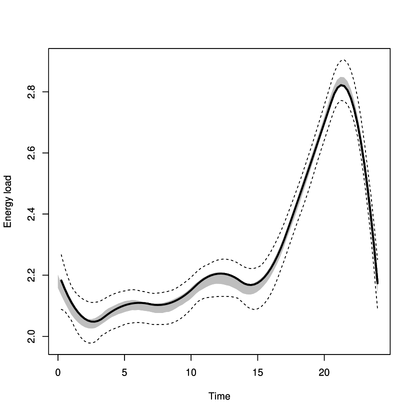
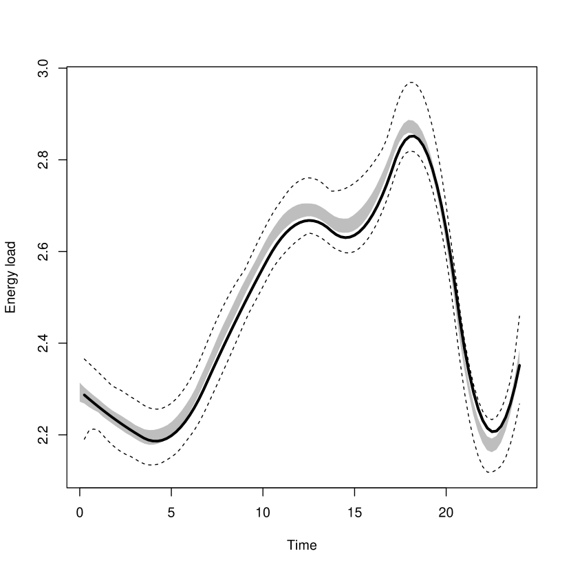
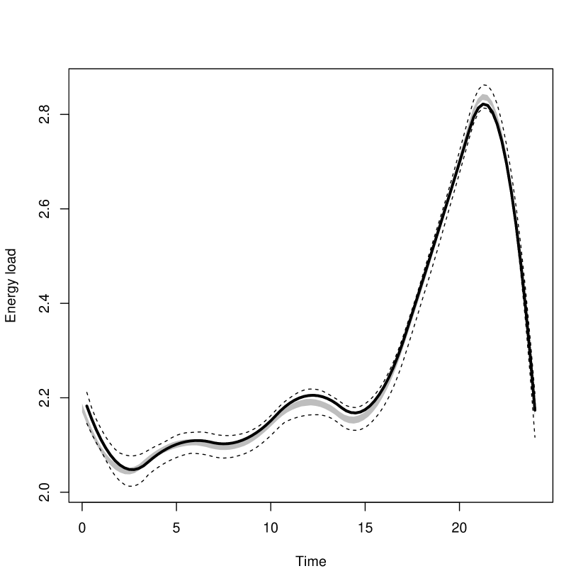
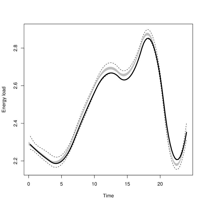
Figure 4: Simulation study Case 1 ($\alpha_{1}$ and $\alpha_{2}$ are of the same scale and the $M$’s are balanced): pointwise minimum, maximum, first and third quartiles of the 200 estimated typologies for classes $c=1$ residential (left column) and $c=2$ commercial (right column) without replicates (top row) and with replicates (bottom row). The solid curve is the true typology used to generate the data, the shaded gray area corresponds to the area between the first and third quartiles and the dashed lines corresponds to the minimum and maximum.

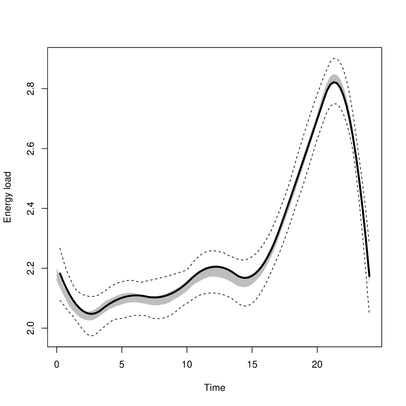
Figure 5: Simulation study Case 2 ($\alpha_{1}$ and $\alpha_{2}$ are of the same scale and the $M_{1}$’s are much bigger than the $M_{2}$’s): pointwise minimum, maximum, first and third quartiles of the 200 estimated typologies for classes $c=1$ residential (left column) and $c=2$ commercial (right column) without replicates (top row) and with replicates (bottom row) as in Figure 4.

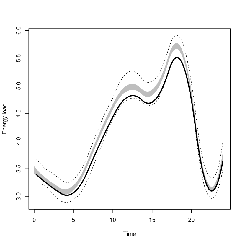
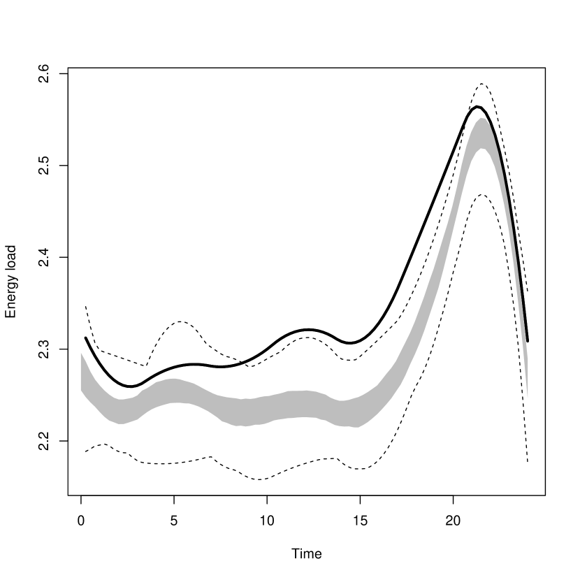
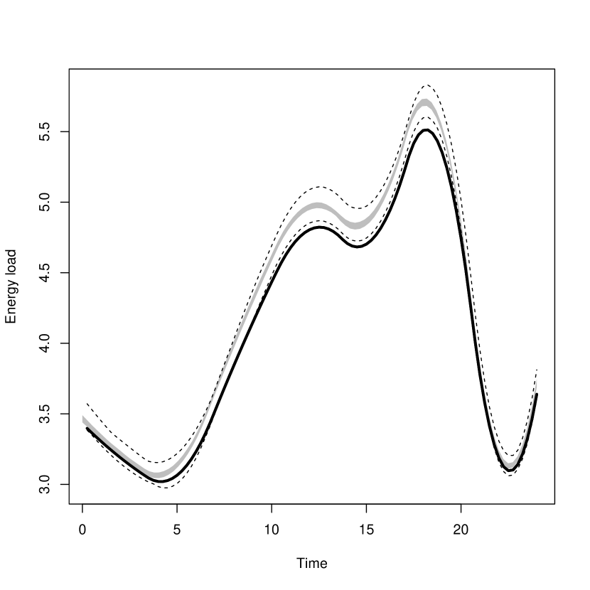
Figure 6: Simulation study Case 3 ($\alpha_{1}$ is much smaller than $\alpha_{2}$ and the $M$’s are balanced): pointwise minimum, maximum, first and third quartiles of the 200 estimated typologies for classes $c=1$ residential (left column) and $c=2$ commercial (right column) without replicates (top row) and with replicates (bottom row) as in Figure 4.

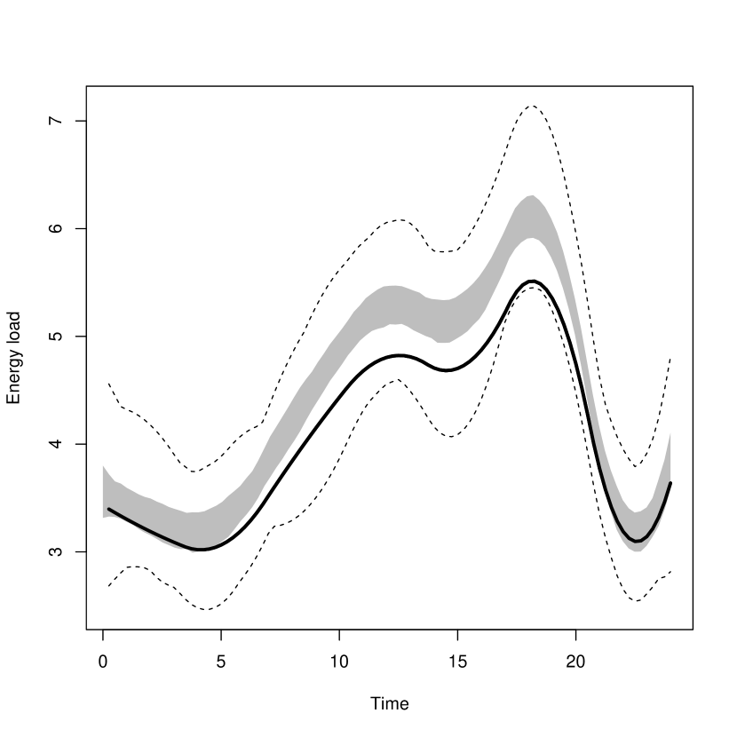
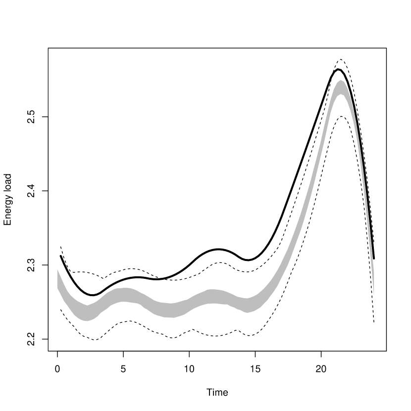
Figure 7: Simulation study Case 4 ($\alpha_{1}$ is much smaller than $\alpha_{2}$ and the $M_{1}$’s are much bigger than the $M_{2}$’s): pointwise minimum, maximum, first and third quartiles of the 200 estimated typologies for classes $c=1$ residential (left column) and $c=2$ commercial (right column) without replicates (top row) and with replicates (bottom row) as in Figure 4.

Figures 4 and 5 show the curves $\alpha_{1}$ and $\alpha_{2}$ for Cases 1 and 2. Figures 6 and 7 present the curves for Cases 3 and 4.

For Cases 3 and 4 we obtain $\alpha_{1}$ and $\alpha_{2}$ along with the corresponding $\mbox{\boldmath{$\gamma$}}^{1}$ and $\mbox{\boldmath{$\gamma$}}^{2}$ by fitting a B-spline model to the data considering a residential class $c=1$ and a commercial class $c=2$. For Cases 1 and 2, we rescale $\alpha_{1}$ and $\alpha_{2}$ by rescaling the associated $\mbox{\boldmath{$\gamma$}}^{1}$ and $\mbox{\boldmath{$\gamma$}}^{2}$ so that all components are between 0 and 1 and the simulated curves are all positive. For instance, to rescale $\alpha_{1}$, let $a_{1}$ equal the minimum of $\mbox{\boldmath{$\gamma$}}^{1}$’s components and $b_{1}$ equal the maximum. We define the rescaled $\alpha_{1}(t)$ as $\mbox{\boldmath{$\phi$}}(t)^{\prime}\mbox{\boldmath{$\gamma$}}^{*1}+2$ with

$$\gamma^{*1}[k]=\frac{\hat{\gamma}^{1}[k]-a_{1}}{b_{1}-a_{1}}.$$ (13)

For the variance parameters for the consumer level energy consumption curves, for Cases 1 and 2, we set $\sigma^{2}_{\gamma,1}$ = 0.03 and $\sigma^{2}_{\gamma,2}$ = 2 $\times$ $\sigma^{2}_{\gamma,1}$ = 0.06. For Cases 3 and 4, to maintain the relative variability of the consumer level curves about the $\alpha_{c}$’s, we rescale $\sigma^{2}_{\gamma,c}$ by multiplying by the appropriate constant: $(b_{c}-a_{c})^{2}$, $c=1,2$. In Cases 1–4, the value of $\sigma_{\gamma,2}^{2}$ is twice $\sigma_{\gamma,1}^{2}$ because we believe that this reflects the variability among commercial consumers compared to the variability among residential consumers.

Figure 8 shows an example of simulated consumer-level data for Case 1 for the first transformer. The left plot shows the energy consumption of 5 out of the 45 consumers of class 1 (residential consumers) and the right plot shows the energy consumption of 5 out of the 30 consumers of class 2 (commercial consumers). Recall that in practice these consumer level consumption curves are not observed: we only observe the sum of all of the 75 curves.

For each of Cases 1–4, we generate two types of data sets: one with just one day observed per transformer and another with five days (replicates) observed per transformer. We generate the days independently, which is a simplification since consumer level day to day usages are probably correlated.

6.2 Analysis and Results

In calculating our estimates, we consider the same fraud matrix $F$ and the same basis functions used to generate data. We also assume that $\Sigma_{c}=\sigma^{2}_{\gamma,c}{\bf I}$ and $\sigma_{i}^{2}=\sigma^{2}$. Recall that for the maximization in Step 2 we require values of the $H$ function given in (8). As described in Section 3.4, we approximate $H$ in each transformer by simulating $B=100,000$ independent data sets just once and tabling the results.

The estimates of $\alpha_{1}$ and $\alpha_{2}$ are summarized in Figures 4-7, which show the pointwise minimum, maximum, median and quartiles of the 200 estimates for each of Cases 1–4. We see that estimates of the $\alpha_{c}$’s are best when the true $\alpha_{c}$’s are of the same scale (Figures 4 and 5). As expected, estimates of the $\alpha_{c}$’s are less variable when they are based on data with replicates (bottom row of plots). When $\alpha_{1}$ is much smaller than $\alpha_{2}$, the estimates are severely biased (Figures 6 and 7). We always obtain excellent estimates of the total electric load for each transformer through the weighted sum $\hat{M}_{1i}\hat{\alpha}_{1}(t)+\hat{M}_{2i}\hat{\alpha}_{2}(t)$, $i=1,\ldots,5$ (e.g., see Figure 9).

Estimates of true consumer counts in the five transformers are provided in Tables 3 and 4 of the supplementary material. The results for transformer $i=2$ are reproduced here in Table 5. The estimates of $M_{1}$ are tabled in the top half of Table 5 for cases with $\alpha_{1}$ and $\alpha_{2}$ of the same scale (Case 1) and of different scales (Case 3), for data with or without replicates. For instance, in the balanced $M$ case (Case 1), transformer 2 contains $M_{1}=$ 29 consumers of class $c=1$, with 32 consumers reporting that they are of class $c=1$. We see that in all cases in this transformer, the most common estimate is $\hat{M}_{1}=31$. We also see that the estimates of $M_{1}$ are more variable for data with no replicates, as expected.

In looking at Tables 3 and 4 of the supplementary material, we see that in all cases, the most common estimate of $M_{1}$ is either at the reported number or at the true value of $M_{1}$ or at some number in between. In many cases, the most common value is equal to the truth, or at least shifted from the reported number towards the truth. Notable exceptions are in transformer 3 in Table 3, when the $M$’s are balanced and in transformers 3, 4 and 5 in Table 4 when the $M$’s are unbalanced. In these exceptions, the most common value of the estimates is the reported number (with one exception). An extreme case of this is in Table 4 (the unbalanced $M$’s case): in transformer 4, our estimates of $M_{1}$ seem “stuck” on the value of the reported number of class 1 consumers. This bias towards the reported number of consumers of class 1 may be due to the fact that, in some cases, the reported number is lower than the true number, which is unusual. As expected, the variability of estimates is always lower when the data contain replicates but, perhaps surprisingly, the bias is not lower.

For variance component estimation, the regression error variance is very well-estimated in all simulation scenarios. However, estimates of the variance parameters of the consumer level energy consumption curves caused some problems, particularly when we observe only one day of data per transformer. In fact, in this case, in many data sets, the estimated consumer level variances are equal to zero.

To investigate the effect of increasing the number of transformers as well as increasing the number of replicates (number of days) we conduct further simulations and present the results in the Supplementary Material. We consider the following scenarios: (i) 5 transformers and 30 days of observation; (ii) 5 transformers and 100 days of observation; (iii) 50 transformers and 1 day of observation; (iv) 50 transformers with 5 days of observation. As expected, the variability of the estimated typologies is reduced by increasing the number of transformers and/or the number of replicates. In addition, the bias in typology estimation is reduced by increasing the number of transformers. Perhaps surprisingly, this bias is not reduced by increasing the number of replicates. Thus, in cases where estimates have a large bias and a decreased variability, the estimated typologies concentrate around the wrong curve. Even with the increase number of replicates and/or number of transformers, in Cases 3 and 4 (when $\alpha_{1}$ is much smaller than $\alpha_{2}$) many estimates of $\sigma_{\gamma,1}^{2}$ were zero. Estimation of $\sigma^{2}$ was good throughout. In general, we found that estimation of $M_{1}$ was as described above: the estimates tended to be shifted from the reported number of consumers of class 1 to the true number. The variability of the estimates decreased with the number of replicates, but surprisingly, not with the number of transformers. The bias typically did not decrease when we increased the number of replicates but did usually decrease with an increase in the number of transformers.

7 Conclusions

In this paper we proposed a generalization of the work of Dias, Garcia and Martarelli (2009) on estimating mean curves when the available sample consists of aggregated functional data. The main novelty of this work is to incorporate a randomness in the counts for class membership. This flexibility allows the analysis of the data even when there is some misreporting in the number of consumers of each type. We also use random effects to model the within transformer correlation structure.

To study the properties of our method, we analyzed artificial data sets exploring different scenarios and we also analyzed a real data set. The artificial data allowed us to explore the influence of increasing the number of replications and the number of transformers. In the data example, it is clear from comparing the observed aggregated curves with the weighted sum of the estimated typical ones, that the proposed model provides reasonable estimates of the mean curve.

Supplementary material

The file supplementary.pdf contains supplementary plots, tables and comparisons for the examples discussed in this paper. It also includes the results of further simulation studies for different numbers of transformers and replicates.

(a) $\hat{\alpha}_{1}$

(b) $\hat{\alpha}_{2}$

(c) $\hat{\alpha}_{3}$

(d) $\hat{\alpha}_{1}$, $\hat{\alpha}_{2}$ and $\hat{\alpha}_{3}$

Figure 2: Data analysis: estimated expected energy consumption, $\hat{\alpha}_{1}$ (residential monophasic), $\hat{\alpha}_{2}$ (residential biphasic) and $\hat{\alpha}_{3}$ (commercial). (a), (b) and (c) show $\hat{\alpha}_{1}$, $\hat{\alpha}_{2}$ and $\hat{\alpha}_{3}$, respectively. (d) shows the three estimated curves together, $\hat{\alpha}_{1}$ (dotted curve), $\hat{\alpha}_{2}$ (solid curve) and $\hat{\alpha}_{3}$ (dashed curve).

(a) Transformer 1

(b) Transformer 2

(c) Transformer 3

Figure 3: Data analysis: observed data and estimated aggregated curves for transformers 1, 2 and 3.

Figure 8: Simulation study Case 1 ($\alpha_{1}$ and $\alpha_{2}$ are of the same scale and the $M$’s are balanced): example of simulated individual level energy consumption curves (dashed curves) for 5 consumers of class 1 (left) and 5 consumers of class 2 (right) compared with the true typical curves (solid line).

Figure 9: Simulation study Case 4 ($\alpha_{1}$ is much smaller than $\alpha_{2}$ and the $M_{1}$’s are much bigger than the $M_{2}$’s): estimate of the total electric load ($\hat{M}_{1i}\hat{\alpha}_{1}(t)+\hat{M}_{2i}\hat{\alpha}_{2}(t)$) for one of the five transformers.

	Monophasic		Biphasic		Commercial
Transformer	Reported	Estimated	Reported	Estimated	Reported	Estimated
1	5	5	29	29	7	7
2	4	4	43	43	3	3
3	48	49	26	25	3	3

Table 1: Data set: reported counts of consumer classes and our estimated counts for the data.

	1	$\cdots$	$j$	$\cdots$	$C$	Row  totals
1	$x_{11}$	$\cdots$	$x_{1j}$	$\cdots$	$x_{1C}$	$M_{1}$
$\vdots$	$\vdots$		$\vdots$		$\vdots$	$\vdots$
$c$	$x_{c1}$	$\cdots$	$x_{cj}$	$\cdots$	$x_{cC}$	$M_{c}$
$\vdots$	$\vdots$		$\vdots$		$\vdots$	$\vdots$
$C$	$x_{C1}$	$\cdots$	$x_{Cj}$	$\cdots$	$x_{CC}$	$M_{C}$
Column  totals	$R_{1}$	$\cdots$	$R_{j}$	$\cdots$	$R_{C}$	$N$

Table 2: Counts of consumer in different categories: $x_{cj}$ is the number of consumers of type $c$ who have reported they are of class $j$.

	$m_{1}$
	25	26	27	28	29	30	31	32	33	34	35	36	37
$\hat{H}$	0.000	0.002	0.007	0.027	0.075	0.166	0.256	0.255	0.143	0.051	0.014	0.003	0.000

Table 3: Estimates of $H(m_{1},75-m_{1})$ when $R_{1}=32$ and $R_{2}=43$ for the fraud matrix in (9).

	Balanced		Unbalanced
Transformer	Truth	Reported	Truth	Reported
1	45	45	66	65
2	29	32	65	66
3	61	60	69	68
4	24	28	62	63
5	12	16	72	71
Total	171	181	334	333

Table 4: Simulation study: the true number of consumers of class 1 and the randomly generated reported number of consumers, as used in the simulation studies. Each transformer served a total of 75 consumers, for a total of 375 consumers.

	${\widehat{M}_{1}}$
Cases	28	${\bf{29}}$	30	31	$[32]$	33
1 without replication	3	24	61	74	35	3
3 without replication	1	7	37	97	55	3
1 with 5 replications	0	0	63	135	2	0
3 with 5 replications	0	0	25	161	14	0

	${\widehat{M}_{1}}$
Cases	64	${\bf{65}}$	$[66]$	67	68
2 without replication	5	63	109	21	2
4 without replication	0	144	56	0	0
2 with 5 replications	0	7	192	1	0
4 with 5 replications	0	170	30	0	0

Table 5: Simulation study: tables of the simulated distribution of $\hat{M}_{1}$, the estimated number of consumers of class $c=1$ (residential) in transformer $i=$2. The top table shows the results for the cases with balanced $M$’s (Cases 1 and 3) and the bottom table shows the results for the cases where all $M_{1}$’s are much larger than the $M_{2}$’s (Cases 2 and 4) . In each table, the column heading contains different possible estimate values with the true value of $M_{1}$ in bold font and the reported value within brackets. Each of the remaining rows corresponds to a different simulation scenario. Each row contains the number of estimates of $M_{1}$ (out of the 200 estimates) that are equal to the associated column heading.

References

- Antoniadis (1994) {bincollection}[author] \bauthor\bsnmAntoniadis, \bfnmAnestis\binitsA. (\byear1994). \btitleWavelet methods for smoothing noisy data. In \bbooktitleWavelets, Images, and Surface Fitting \bpages21–28. \bpublisherA K Peters. \bmrnumberMR1302234 \endbibitem
- Bodin, Villemoes and Wahlberg (2000) {barticle}[author] \bauthor\bsnmBodin, \bfnmPer\binitsP., \bauthor\bsnmVillemoes, \bfnmLars F.\binitsL. F. and \bauthor\bsnmWahlberg, \bfnmBo\binitsB. (\byear2000). \btitleSelection of best orthonormal rational basis. \bjournalSIAM Journal on Control and Optimization \bvolume38 \bpages995–1032 (electronic). \bmrnumberMR1760057 (2001j:42019) \endbibitem
- Cardoso (1998) {barticle}[author] \bauthor\bsnmCardoso, \bfnmJean-François\binitsJ.-F. (\byear1998). \btitleBlind signal separation: statistical principles. \bjournalProceedings of the IEEE. Special Issue on Blind Identification and Estimation \bvolume9 \bpages2009-2025. \endbibitem
- Choi et al. (2005) {barticle}[author] \bauthor\bsnmChoi, \bfnmSeungjin\binitsS., \bauthor\bsnmCichocki, \bfnmAndrzej\binitsA., \bauthor\bsnmPark, \bfnmHyung-Min\binitsH.-M. and \bauthor\bsnmLee, \bfnmSoo-Young\binitsS.-Y. (\byear2005). \btitleBlind source separation and independent component analysis: a review. \bjournalNeural Information Processing - Letters and Reviews \bvolume6 \bpages1–57. \endbibitem
- Comon and Jutten (2010) {bbook}[author] \bauthor\bsnmComon, \bfnmPierre\binitsP. and \bauthor\bsnmJutten, \bfnmChristian\binitsC. (\byear2010). \btitleHandbook of Blind Source Separation: Independent Component Analysis and Applications, \bedition1st ed. \bpublisherAcademic Press. \endbibitem
- De Vore, Petrova and Temlyakov (2003) {barticle}[author] \bauthor\bsnmDe Vore, \bfnmRonald\binitsR., \bauthor\bsnmPetrova, \bfnmGuergana\binitsG. and \bauthor\bsnmTemlyakov, \bfnmVladimir\binitsV. (\byear2003). \btitleBest basis selection for approximation in . \bjournalFoundations of Computational Mathematics \bvolume3 \bpages161–185. \bmrnumberMR1966298 (2004c:41033) \endbibitem
- Dias (1998) {barticle}[author] \bauthor\bsnmDias, \bfnmRonaldo\binitsR. (\byear1998). \btitleDensity estimation via hybrid splines. \bjournalJournal of Statistical Computation and Simulation \bvolume60 \bpages277–294. \endbibitem
- Dias, Garcia and Martarelli (2009) {barticle}[author] \bauthor\bsnmDias, \bfnmRonaldo\binitsR., \bauthor\bsnmGarcia, \bfnmNancy Lopes\binitsN. L. and \bauthor\bsnmMartarelli, \bfnmAngelo\binitsA. (\byear2009). \btitleNon-parametric estimation for aggregated functional data for electric load monitoring. \bjournalEnvironmetrics \bvolume20 \bpages111–130. \endbibitem
- Dias, Garcia and Schmidt (2013) {barticle}[author] \bauthor\bsnmDias, \bfnmRonaldo\binitsR., \bauthor\bsnmGarcia, \bfnmNancy Lopes\binitsN. L. and \bauthor\bsnmSchmidt, \bfnmAlexandra Mello\binitsA. M. (\byear2013). \btitleA hierarchical model for aggregated functional data. \bjournalTechnometrics \bvolume55 \bpages321-334. \endbibitem
- Gu (1993) {barticle}[author] \bauthor\bsnmGu, \bfnmChong\binitsC. (\byear1993). \btitleSmoothing spline density estimation: a dimensionless automatic algorithm. \bjournalJournal of the American Statistical Association \bvolume88 \bpages495-504. \endbibitem
- Kohn, Marron and Yau (2000) {barticle}[author] \bauthor\bsnmKohn, \bfnmRobert\binitsR., \bauthor\bsnmMarron, \bfnmJ. S.\binitsJ. S. and \bauthor\bsnmYau, \bfnmPaul\binitsP. (\byear2000). \btitleWavelet estimation using Bayesian basis selection and basis averaging. \bjournalStatistica Sinica \bvolume10 \bpages109–128. \bmrnumberMR1742103 (2000k:62086) \endbibitem
- Kooperberg and Stone (1991) {barticle}[author] \bauthor\bsnmKooperberg, \bfnmCharles\binitsC. and \bauthor\bsnmStone, \bfnmCharles J.\binitsC. J. (\byear1991). \btitleA study of logspline density estimation. \bjournalComputational Statistics and Data Analysis \bvolume12 \bpages327–347. \endbibitem
- Luo and Wahba (1997) {barticle}[author] \bauthor\bsnmLuo, \bfnmZhen\binitsZ. and \bauthor\bsnmWahba, \bfnmGrace\binitsG. (\byear1997). \btitleHybrid adaptive splines. \bjournalJournal of the American Statistical Association \bvolume92 \bpages107–116. \endbibitem
- Wahba (1983) {barticle}[author] \bauthor\bsnmWahba, \bfnmG.\binitsG. (\byear1983). \btitleBayesian “confidence intervals” for the cross-validated smoothing spline. \bjournalJournal of the Royal Statistical Society Series B \bvolume45 \bpages133–150. \endbibitem