Non-collinear magnetism induced by frustration in transition-metal nanostructures deposited on surfaces

Abstract

How does magnetism behave when the physical dimension is reduced to the size of nanostructures? The multiplicity of magnetic states in these systems can be very rich, in that their properties depend on the atomic species, the cluster size, shape and symmetry or choice of the substrate. Small variations of the cluster parameters may change the properties dramatically. Research in this field has gained much by the many novel experimental methods and techniques exhibiting atomic resolution. Here I review the ab-initio approach, focusing on recent calculations on magnetic frustration and occurrence of non-collinear magnetism in antiferromagnetic nanostructures deposited on surfaces.

I Introduction

Atomic and nanometer scale magnetism - in short called nanomagnetism - stands as one of the frontier fields in magnetism. Nanomagnetism opens on one hand new vistas to magnetic storage media, on the other hand it is a largely unexplored area of physics where novel effects ought to be expected. Controlling the flow of magnetic and charge information between increasingly smaller structures hinges on the meticulous control of the coupling between spins. Obviously, this is of central importance for the design of novel devices engineered on the level of individual atomic spins sarma whose functionality is geared towards computing speed, storage capacity and energy saving. Unprecedented opportunities for atomic engineering of future spintronics and quantum information devices arise thanks to fundamental explorations of magnetic nanochains and nanostructures using advanced experimental methods (see e.g. Refs. crommie ; mirkovic ; rusponi ; stroscio ; wurth ; hirjibehedin ; wiebe ; wiebe2 ; wiebe3 ; wulfhekel ; heinze ; loth ).

By means of the scanning tunneling microscope (STM), nanostructures are built atom by atom on different kind of substrates in controlled processes, resulting in well-defined magnetic units on the nano-scale. For example, logic gates based on magnetic nanochains were recently built alex_science while even the magnetic exchange interactions between adatoms could be evaluated quantitatively using STM wiebe ; wiebe3 . Moreover a recently developed technique, inelastic scanning tunneling spectroscopy (ISTS), allowed access of spin excitations with STM. Thus values of the magnetic anisotropy energy and magnetic properties of nanostructures down to single adatoms are measured experimentally and simulated theoretically (see for example Refs. hirjibehedin ; wulfhekel2 ; khajetoorians ; persson ; fernandez-rossier ; lorente ; lounis_ists ). The properties of the magnetic nano-objects crucially depend on the atom species, the cluster shape and size and on the substrate material, magnetization and surface orientation. Therefore, there are numerous properties and effects, the understanding of which requires an interdisciplinary theoretical approach by ab-initio electronic structure methods, simplifying models, and statistical-mechanical methods, which together with experiment serve the goal of a description and a qualitative understanding of magnetic nano-structures (see e.g. Refs. smogunov ; carbone ; lazarovitz ; mokrousov ; lagoute ; ebert ; mavropoulos ; klautau

Among the manifestations of magnetic complexity, perhaps most striking is the phenomenon of non-collinear magnetism, i.e., the case when the magnetic moments of atoms in a system are oriented in different directions. Far from paramagnetism, which occurs in the limit of vanishing inter-atomic interactions, here we are faced with particularly strong nearest-neighbor magnetic-moment coupling, reaching the order of magnitude of 0.5 eV, with non-collinearity being the result of competition among interactions. Basically, there are two types of competition. The first comes from direct antiferromagnetic exchange, with the competing interactions being of the same order of magnitude and the non-collinearity arising in a nearest-neighbor length scale. This effect is usually termed as frustration and will be the main topic of discussion in the present paper. The second is a competition of direct exchange with anisotropic exchange which arises from spin-orbit coupling and is typically at least an order of magnitude weaker. It leads to longer-range manifestation of non-collinear magnetism, typically on a length-scale of a few interatomic distances or more. Here we will simply reference works that have studied the latter, while our focus is on the former.

Magnetic frustration denotes the inability to satisfy competing exchange interactions between neighboring atoms. A simple model for frustration is the following (see Fig. 1), based on the antiferromagnetic (AF) interaction among neighboring Cr atoms. Starting with an antiferromagnetic (AF) Cr dimer, the addition of a third Cr atom to form an equilateral triangle leads to a frustrated geometry. Each atomic moment tends to be aligned AF to both its neighbors. Since this is impossible, the moments of the three atoms relax in a state of compromise. The ground state is then non-collinear, characterized by an angle of 120^∘ between each two atoms. The number of non-collinear solutions that share this property is infinite, since if all moments are rotated by the same angle their relative orientation to each other does not change. On the other hand, interaction with a magnetic substrate of a fixed-moment orientation stabilizes only one or perhaps a few of these infinitely many states.

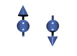
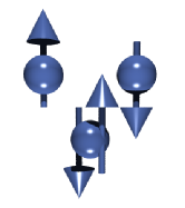
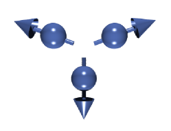
A                               B                               C

Figure 1: Example of frustration seen with an antiferromagnetic Cr dimer (A) to which we add a third equidistant atom. A magnetically frustrated state is obtained (B) because all three atoms tend to couple antiferromagnetically to each other leading then to a non-collinear magnetic structure (C) as a ground state.

This Neel state is an example of intra-cluster frustration that can occur in clusters deposited on non-magnetic surfaces with a triangular symmetry such as fcc(111) surfaces bergman ; demangeat ; costa ; stocks ; gotsis ; antal ; bergman_gold ; klautau_pt ; nikos (e.g. Cu(111), Au(111) or Pt(111)). On magnetic surfaces, however, the non-collinear state can be also realized without intra-cluster frustration if there is a competition between the intra-cluster interactions, on the one hand, and the cluster-substrate interactions, on the other lounis05 ; lounis07 ; lounis08 ; lounis_prl ; wulfhekel . We call such a situation a cluster-substrate frustration, which as we shall see can also lead to complex magnetic behavior.

In fact, it is helpful in general to distinguish between three factors contributing to the equilibrium magnetic state:
(i) the pair interaction among the atoms in the cluster,
(ii) the interaction of the cluster atoms with the substrate, and
(iii) the geometry of the cluster (which is fixed by the substrate).
This separation is meaningful because the nearest-neighbors exchange interaction is energetically dominant compared to second, third, etc. neighbors, and because in different cluster sizes or shapes the type of pair interaction (ferro- or antiferromagnetic) does not change qualitatively. Quantitatively, however, this is only an approximation, and effects beyond this occur which are computed during the self-consistent calculations presented in this Highlight.

A first approximation to a description of magnetic frustration phenomena can be achieved by employing a classical Heisenberg Hamiltonian of the form

$$H=-\frac{1}{2}\sum_{i\neq j}{J}_{ij}{\vec{e}_{i}\cdot\vec{e}_{j}}.$$ (1)

Here, $\vec{e}_{i}$ is a unit vector defining the direction of the magnetic moment and $i$ and $j$ indicate the magnetically involved atoms, including the substrate atoms. The sign and strength of the terms $J_{ij}$ (where the magnitude of the moments has been absorbed) define the ground state. Spin-orbit interaction could lead to non-collinear magnetism and recently it has been shown that anti-symmetric type of interactions, called the Dzyaloshinskii-Moriya interactions dzialoshinskii could occur on surfaces heide_nature ; heide_prb ; szunyogh_prl or even nanostructures on surfaces ebert_prl ; antal ; ebert ; Bauer . These kind of interactions, reviewed in Ref. heide_highlight , can of course easily be included in the previous Heisenberg Hamiltonian by terms of the form $\vec{D}_{ij}\cdot\vec{e}_{i}\times\vec{e}_{j}$. Henceforth, however, we limit our discussion to the physics of finite nanostructures where the spin-orbit coupling is negligible.

One way to proceed is to derive the values of $J_{ij}$ from density-functional calculations at a particular (e.g. collinear ferromagnetic) state lichtenstein (see also Refs.bruno ; lounis_jij ; szilva ), and then find the energy minimum using Eq. (1). This is probably a good approximation under the condition that the magnitude of the moments does not depend strongly on the relative direction to the neighboring moments, and that no higher-order corrections to the energy are necessary. These conditions are usually met in systems where the direction of the moments varies in a length-scale of several inter-atomic distances, for example in the case of spin-orbit-induced non-collinear states, or in the case of low-energy magnetic excitations. Here, however, we are faced with strong directional fluctuations between neighboring moments, and it turns out that the conditions are not met. In addition, as we shall see, there occur more than one energy minima that are not reproduced by the Heisenberg model. Therefore one has to proceed by doing a full self-consistent calculation of the non-collinear state, using the Heisenberg model only as guideline.

Part of the reason that the Heisenberg Hamiltonian (1) fails is that we have in mind $3d$ transition elements. These are characterized by $d$ orbitals localized enough to produce a magnetic moment, but also delocalized enough to provide strong exchange interactions. Precisely this delocalization of the orbitals, creating itinerant states, has as a consequence that the electronic structure of an atom is affected by the magnetic orientation of its neighbors. Most susceptible to changes are actually the early and middle transition elements, e.g. V or Cr, due to their more delocalized $d$ orbitals compared to the Mn or later elements where the $d$ orbitals are deeper in the potential well; and also Ni, because of the low-energy scale of its magnetic moment.

The correlation function $\chi_{ij}$, i.e., the response of the moment at site $i$ to a rotation of the moment at $j$, is long-ranged. As a consequence, adding one magnetic atom at the boundary of a non-collinear nanostructure can change the whole state. Experimentally this can be achieved by moving a surface-adsorbed atom by an STM tip, as shown schematically in Fig. 2. We will see that such manipulations can lead to interesting even-odd effects, depending on the size and shape of the nanostructure.

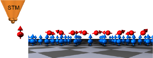
Figure 2: A STM tip moving an adatom towards a nanochain.

Most of the presented results are on magnetic surfaces, although some of the work carried out on non-magnetic surfaces is briefly discussed. The choice of cluster-atoms, substrate materials and surface orientations is motivated mainly according to points (i)-(iii) discussed earlier. Basically Cr and Mn are excellent candidates for the cluster because of their antiferromagnetic nature. Fe and Ni provide substrates with different strength of exchange interaction with the cluster. Finally, the fcc(111) and (001) surfaces provide different geometry types, the former inducing an intra-cluster frustration due to its triangular geometry, the latter not.

Two of the studied magnetic surfaces have non-triangular symmetry, thus frustration is induced by the interaction with the magnetic substrate. These are of fcc(001) type: Ni(001) and Fe_3ML/Cu(001) surface. The former surface provides a smaller magnetic coupling to the ad-clusters compared to the latter one. Fe_3ML/Cu(001) substrate, known to be ferromagnetic up to four Fe monolayers thomassen ; asada ; stepanyuk1 ; moroni , was chosen since it was used for x-ray magnetic circular dichroism measurements on Cr ad-clusters. The third surface is Ni(111) where the surface geometry is triangular, meaning, in terms of magnetic coupling, that a compact trimer with antiferromagnetic interactions resting on the surface necessarily suffers magnetic frustration. This frustration leads to the well-known non-collinear Neel states being characterized by 120^∘ angles between the moments. Hence, in such a system we face an interplay between the non-collinear coupling tendencies arising from the interaction among the adatoms in the cluster and the collinear tendencies arising from the additional coupling to the substrate atoms. This is very different to the Ni(001) or Fe_3ML/Cu(001) surfaces where the frustration and non-collinear state arises from the competition between the coupling in the cluster and with the substrate.

The majority of the ab-initio methods available for the treatment of non-collinear magnetism make explicit use of Bloch’s theorem and are thus restricted to periodic systems (bulk or films). Then one needs large supercells to simulate impurities in a given host (bulk or film) in order to avoid spurious interactions of the impurities from adjacent supercells. In contrast, the Korringa-Kohn-Rostoker Green function (KKR) method does not require a supercell which makes it an ideal tool to nanostructures on surfaces. Indeed since the method is based on Green functions, a real-space approach can elegantly be used papanikolaou ; ebert_highlight (see Fig. 3).

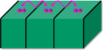
(a) (b)

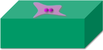
Figure 3: Adatoms on surface. In (a) the supercell approach is depicted with arrows showing the spurious interaction between nanostructures of adjacent supercells. This unwanted interaction is avoided in the real-space KKR formalism (b).

First non-collinear calculations by the KKR Green function method, though not self–consistent, were already performed in 1985. Oswald et al. oswald0 could show by using the method of constraints that the exchange interaction between the moments of Mn and Fe impurity pairs in Cu is in good approximation described by the $\cos\theta$–dependence of the Heisenberg model.

Sandratskii et al. sandratskii1 and Kübler et al. kuebler1 ; kuebler2 pioneered the investigation of non-collinear magnetic structures using self–consistent density functional theory and investigated the spin spiral of bcc Fe with the KKR method. Later on, $\Delta$-Fe was a hot topic, and the appearance of the experimental work of Tsunoda et al. tsunoda1 ; tsunoda2 led to the development of other first–principles methods able to deal with non-collinear magnetism such as LMTO mryasov , ASW knoepfle and FLAPW. kurz ; nordstroem ; sjoestedt

Several papers sandratskii2 ; sandratskii3 describe how symmetry simplifies the computational effort for the spiral magnetic structures in the case of perfect periodic systems—this involves the generalized Bloch theorem. In ab-initio methods, this principle is used together with the constrained density functional theory dederichs ; grotheer giving the opportunity of studying arbitrary magnetic configurations where the orientations of the local moments are constrained to nonequilibrium directions.

Concerning unsupported clusters, few methods are developed. For example, Oda et al. oda developed a plane-wave pseudopotential scheme for non-collinear magnetic structures. They applied it to small Fe clusters for which they found non-collinear magnetic structures for Fe₅ and linear-shape Fe₃. This last result was in contradiction with the work of Hobbs et al. hobbs who found only a collinear ferromagnetic configuration using a projector augmented-wave method. Small Cr clusters were found magnetically non-collinear, oda as shown also by Kohl and Bertsch kohl using a relativistic nonlocal pseudopotential method.

One main result of Oda et al. oda and Hobbs et al. hobbs concerns the variation of the magnetization density with the position. The spin direction changes in the interstitial region between the atoms where the charge and magnetization densities are small, while the magnetization is practically collinear within the atomic spheres. This supports the use of a single spin direction for each atomic sphere as an approximation in order to accelerate the computation; this approximation is followed also here.

II Theory: Non-collinear KKR formalism

The KKR method uses multiple-scattering theory in order to determine the one-electron Green function in a mixed site and angular–momentum representation. In the simple case of collinear magnetism, the retarded Green function is spin-diagonal, $G=\text{diag}(G_{\uparrow},G_{\downarrow})$, and is expanded as:

$${G}_{s}(\vec{R}_{n}+\vec{r},\vec{R}_{n^{\prime}}+\vec{r}^{\prime};E)=-i\sqrt{E}\sum_{L}{R}_{Ls}^{n}({\vec{r}_{<}};E){H}_{Ls}^{n}({\vec{r}_{>}};E)\delta_{nn^{\prime}}+\sum_{LL^{\prime}}{R}_{Ls}^{n}({\vec{r}};E){G}_{s;LL^{\prime}}^{nn^{\prime}}(E){R}_{L^{\prime}}^{n^{\prime}}({\vec{r}^{\prime}};E)$$ (2)

Here, $E$ is the energy and $\vec{R}_{n}$, $\vec{R}_{n^{\prime}}$ refer to the atomic nuclei positions. By $\vec{r}_{<}$ and $\vec{r}_{>}$ we denote respectively the shorter and longer of the vectors $\vec{r}$ and $\vec{r}^{\prime}$ which define the position in each Wigner–Seitz cell relative to the position $\vec{R}_{n}$ or $\vec{R}_{n^{\prime}}$. The wavefunctions ${R}_{sL}^{n}(\vec{r};E)$ and ${H}_{sL}^{n}(\vec{r};E)$ are, respectively, the regular and irregular solutions of the Schrödinger equation for the potential $V_{sn}$ at site $n$, being embedded in free space; $L=(l,m)$ is a combined index for angular momentum quantum numbers; $l$ is truncated at a maximum value of $l_{\mathrm{max}}$. The first term on the RHS of Equation (2) is the so-called single site scattering term, which describes the behavior of an atom $n$ in free space. All multiple-scattering information is contained in the second back-scattering term via the structural Green functions ${G}_{s;LL^{\prime}}^{nn^{\prime}}(E)$ which are obtained by solving the algebraic Dyson equation:

$${G}_{s;LL^{\prime}}^{nn^{\prime}}(E)=\mathring{G}^{nn^{\prime}}_{s;LL^{\prime}}(E)+\sum_{n^{\prime\prime},L^{\prime\prime}L^{\prime\prime\prime}}\!\!\!\!\!\mathring{G}_{s;LL^{\prime\prime}}^{nn^{\prime\prime}}(E){\Delta t}_{s;L^{\prime\prime}L^{\prime\prime\prime}}^{n^{\prime\prime}}(E){G}_{s;L^{\prime\prime\prime}L^{\prime}}^{n^{\prime\prime}n^{\prime}}(E)$$ (3)

Equation (3) follows directly from the usual Dyson eq. of the form $G_{s}=\mathring{G}_{s}+\mathring{G}_{s}\,\Delta V_{s}\,G_{s}$, with $\Delta V_{s}$ the perturbation in the potential for spin $s$ and $\mathring{G}_{s}$ the Green function for some already solved reference system. The summation in (3) is over all lattice sites $n^{\prime\prime}$ and angular momenta $L^{\prime\prime}$ for which the perturbation ${\Delta t}_{L^{\prime\prime}L^{\prime\prime\prime}}^{n^{\prime\prime}}(E)={t}_{L^{\prime\prime}L^{\prime\prime\prime}}^{n^{\prime\prime}}(E)-\mathring{t}_{L^{\prime\prime}L^{\prime\prime\prime}}^{n^{\prime\prime}}(E)$ between the ${t}$ matrices of the real and the reference system is significant (the $t$-matrix gives the scattering amplitude of the atomic potential). The quantities $\mathring{G}_{s;LL^{\prime}}^{nn^{\prime}}(E)$ are the structural Green functions of the reference system. For the calculation of a crystal bulk or surface, the reference system can be free space, or, within the screened KKR formulation SKKR , a system of periodically arrayed repulsive potentials. After the host (bulk or surface) Green function is found, it can be used in a second step as a reference for the calculation in real space of the Green function of an impurity or a cluster of impurities embedded in the host.

The algebraic Dyson equation (3) is solved by matrix inversion, as we will see later on in Equation (7). In case of spin-dependent electronic structure, spin indices enter in the $t$-matrix, the Green functions and in Eq. (3). Especially in the case of non-collinear magnetism, these quantities become $2\times 2$ matrices in spin space, denoted by $\boldsymbol{t}$ and $\boldsymbol{G}$ (see for example Refs. lounis05 or mertig ).

Once the spin-dependent Green function is known, all physical properties can be derived from it. In particular, the charge density $n(\vec{r})$ and spin density $\vec{m}(\vec{r})$ are given by an integration of the imaginary part of $\boldsymbol{G}$ up to the Fermi level $E_{F}$ and a trace over spin indices $s$ (putting the Green function in a matrix form in spin space):

$$n(\vec{r}) = -\frac{1}{\pi}\mathrm{Im}\mathrm{Tr}_{s}\int^{E_{F}}\boldsymbol{G}(\vec{r},\vec{r};E)\,dE$$ (4)

$$\vec{m}(\vec{r}) = -\frac{1}{\pi}\mathrm{Im}\mathrm{Tr}_{s}\int^{E_{F}}\vec{\boldsymbol{\sigma}}\,\boldsymbol{G}(\vec{r},\vec{r};E)\,dE.$$ (5)

Here, $\vec{\boldsymbol{\sigma}}=(\boldsymbol{\sigma}_{x},\boldsymbol{\sigma}_{y},\boldsymbol{\sigma}_{z})$ are the Pauli matrices.

The basic difference between non-collinear and collinear magnetism is the absence of a natural spin quantization axis common to the whole crystal. The density matrix is not anymore diagonal in spin space as in the case of collinear magnetism. Instead, in any fixed frame of reference it has the form

$$\boldsymbol{\rho}(\vec{r})=\begin{bmatrix}{\rho}_{\uparrow\uparrow}(\vec{r})&{\rho}_{\uparrow\downarrow}(\vec{r})\\ {\rho}_{\downarrow\uparrow}(\vec{r})&{\rho}_{\downarrow\downarrow}(\vec{r})\end{bmatrix}=\frac{1}{2}\left[n(\vec{r})+\vec{\boldsymbol{\sigma}}\cdot\vec{m}(\vec{r})\right]$$ (6)

At any particular point in space, of course, a local frame of reference can be found in which $\boldsymbol{\rho}$ is diagonal, but this local frame can change from point to point.

The KKR Green function ansatz for non-collinear magnetism is analogous to (2), but including non-spin-diagonal elements $ss^{\prime}$ lounis05 . A simplification is achieved by an approximation to the exchange-correlation potential which is assumed to be collinear within each atomic cell [by averaging the direction of the non-collinear exchange-correlation potential $\vec{B}_{\rm xc}(\vec{r})$], accelerating computational time of the single-site solutions and reducing the number of iterations. Then for each cell we define a local reference frame with respect to which the local solutions of the Schrödinger equation and the $t$-matrix, $\boldsymbol{t}^{\rm loc}_{n}$, are spin-diagonal. After the local Schrödinger equation is solved, the $t$-matrix of each atom is rotated in spin-space to a pre-defined global frame by a site-dependent transformation in spin space, $\boldsymbol{t}^{\rm glob}_{n}=\boldsymbol{U}_{n}\boldsymbol{t}^{\rm loc}_{n}\boldsymbol{U}_{n}^{\dagger}$. The resulting matrix $t_{n;ss^{\prime}}$ is not any more spin-diagonal (but always site-diagonal), with the non-diagonal terms containing the information on spin-flip scattering by the atomic potential. From $\boldsymbol{t}^{\rm glob}_{n}$, and from the reference-system structural Green function, we calculate, just as in the collinear case, the structural Green function of the perturbed system by solving the algebraic Dyson equation, where now all objects are matrices in terms of site, angular momentum, and spin index:

$$\boldsymbol{G}_{\mathrm{str}}(E)=\mathring{\boldsymbol{G}}_{\mathrm{str}}(E)[1-\Delta\boldsymbol{t}^{\mathrm{\text{glob}}}(E)\,\mathring{\boldsymbol{G}}_{\mathrm{str}}(E)]^{-1}.$$ (7)

In order to obtain the output charge- and spin-density, the local wavefunctions ${R}_{sL}^{n}(\vec{r};E)$ and ${H}_{sL}^{n}(\vec{r};E)$ are also projected to the global frame using the projection matrices $\boldsymbol{\sigma}_{ns}$ for the local spin–up ($\uparrow$) and spin–down ($\downarrow$) directions:

$$\boldsymbol{\sigma}_{ns}=\frac{1}{2}\boldsymbol{U}_{n}(\boldsymbol{1}\pm\boldsymbol{\sigma}_{z})\boldsymbol{U}^{{\dagger}}_{n}=(\boldsymbol{\sigma}_{ns})^{2}\ \ \ (\mbox{$+$ for $s=\uparrow$, $-$ for $s=\downarrow$})$$ (8)

Then we have:

$$\boldsymbol{G}^{\text{glob}}(\vec{R}_{n}+{\vec{r}},\vec{R}_{n^{\prime}}+{\vec{r}^{\prime}};E)=-i\sqrt{E}\sum_{Ls}{R}^{\text{loc}}_{nLs}({\vec{r}_{<}};E){H}^{\text{loc}}_{nLs}({\vec{r}_{>}};E)\boldsymbol{\sigma}_{ns}$$

$$+\sum_{LL^{\prime}ss^{\prime}}{R}^{\text{loc}}_{nLs}({\vec{r}};E)\boldsymbol{\sigma}_{ns}\boldsymbol{G}^{\text{glob}}_{LL^{\prime}nn^{\prime}}(E)\boldsymbol{\sigma}_{n^{\prime}s^{\prime}}{R}^{\text{loc}}_{n^{\prime}L^{\prime}s^{\prime}}({\vec{r}^{\prime}};E).$$ (9)

At the end, given the spin-density, an average is made in order to define the new site-dependent local axis $(\theta_{n},\phi_{n})$ with respect to the global reference frame:

$${\tan}{\theta}_{n}=\frac{\int_{\mathrm{WS}}{m}^{z}_{n}({\vec{r}})d{\vec{r}}}{\int_{\mathrm{WS}}{m}_{n}({\vec{r}})d{\vec{r}}},\ \ \ {\tan}{\phi}_{n}=\frac{\int_{\mathrm{WS}}{m}^{y}_{n}({\vec{r}})d{\vec{r}}}{\int_{\mathrm{WS}}{m}^{x}_{n}({\vec{r}})d{\vec{r}}}.$$ (10)

In order to find the output exchange-correlation potential within the local spin-density approximation, the spin density of each atom is projected on its local-frame direction $(\theta_{n},\phi_{n})$ and the self-consistency cycle is repeated in the usual density-functional theory sense.

III 3d single adatoms and inatoms

In order to understand the behavior of complex nanostructures it is necessary to investigate their building block that are adatoms and inatoms (i.e., impurity atoms in the first surface layer). Here we would like to review the behavior of 3$d$ adatoms on the three chosen ferromagnetic surfaces, Ni(001) (see for example Refs. nonas ; nonas1 ; nonas2 ; nonas3 ; lounis05 ), Fe_3ML/Cu(001) lounis08 and Ni(111) lounis07 .

By comparing the energies of the FM solution, where the adatom moment is parallel to the surface-atom moments, with the AF solution, where the relative orientation is of antiferromagnetic type, we find the first elements of the 3d series (Sc, Ti, V, Cr) are AF whereas Mn, Fe, Co and Ni are FM. This is is shown in Fig. 4(a) where the energy difference between the AF and FM solutions is plotted.

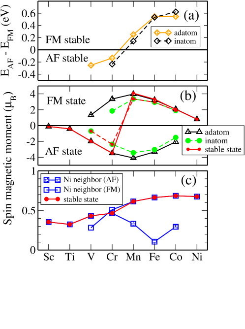
Figure 4: 3d adatoms and inatoms on Ni(001): (a) Energy difference between the AF and FM solutions. The values related to adatom and inatoms are described by respectively full and empty black diamonds. (b) Magnetic moments of the adatoms (black triangles) and inatoms (green circles) within the two possible magnetic configurations FM and AF. (c) Variation of the magnetic moments of Ni nearest neighbors of the adatoms. Adapted with permission from Ref.lounis05 .

Clearly, the AF-FM transition occurs when the adatom atomic number changes from Cr ($Z=24$) to Mn ($Z=25$). lounis05 This transition can be interpreted as in the case of the interatomic interaction of magnetic dimers anderson ; oswald , in terms of the energy gain due to the formation of hybrid states with the Ni substrate as the $3d$ virtual bound state (VBS) comes lower in energy with increasing $Z$ (see Fig. 5). Energy is gained when a half-occupied d VBS at $E_{F}$ is broadened by hybridization with the Ni minority 3d states, which lie at $E_{F}$ (the Ni majority d states are fully occupied and positioned below $E_{F}$). This mechanism is called double exchange (the term is borrowed from the magnetism of transition-element impurities in oxides, since the mechanism is similar). For the early 3d adatoms (Fig. 5a), it is the majority d VBS which is at $E_{F}$, thus the majority–spin direction of the adatom is favorably aligned with the minority–spin direction of Ni, and an AF coupling arises. For the late 3d adatoms (Fig. 5b), on the contrary, the minority d VBS is at $E_{F}$, and this aligns with the Ni minority d states; then a FM coupling arises. For our purposes we keep in mind that, since Cr and Mn are in the intermediate region, i.e., near the AF-FM transition point, their magnetic coupling to the Ni substrate is weak; this has consequences to be seen in the behavior of dimers, trimers, etc., in the next sections.

We should also stress the importance of kinetic exchange, which produces antiferromagnetic coupling, and occurs when occupied states of one atom hybridize with unoccupied states of its neighbor. This situation, demonstrated in Fig. 5, leads to a down-shifting of the occupied levels, gaining energy. Contrary to this, a parallel alignment does not lower the energy, since there is no level shifting, but only level broadening of majority VBS. Since these are fully occupied, the broadening brings no energy gain. This is the reason that Cr and Mn neighboring atoms couple antiferromagnetically anderson ; oswald .

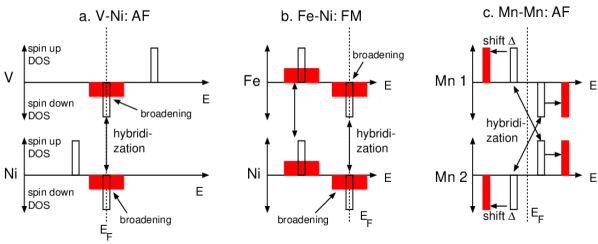
Figure 5: Alexander–Anderson model for neighboring magnetic atoms: (a) Early 3d transition elements in interaction with Ni surface atoms (double exchange); (b) Late 3d transition elements in interaction with Ni surface atoms (double exchange); (c) Cr or Mn dimer (kinetic exchange). Adapted with permission from Ref.lounis05 .

The magnetic moments of the adatoms and Ni nearest neighbors in the surface layer are shown in Fig. 4(b) and (c). Evidently the moment of the Ni nearest neighbors is strongly affected by the adatoms. Especially for Mn, Fe, and Co adatoms, where the FM configuration is stable, the Ni moment is strongly in the AF state. As regards the adatom moments, the half filled $d$ VBS, together with Hund’s rule, cause the Mn adatom to carry the highest magnetic moment (4.09 $\mu_{B}$) followed by Cr (3.48 $\mu_{B}$) and Fe (3.24$\mu_{B}$).

To understand the effect of coordination and stronger hybridization on the magnetic behavior of the adatoms, we take the case of impurities sitting in the first surface layer (inatoms). We carried out the calculations for V, Cr, Mn, Fe and Co impurities. The corresponding spin moments are shown in Fig. 4b (green circles), and the FM-AF energy differences are shown in Fig. 4a (open diamonds and dashed line). Compared to the adatom case, the spin moments are reduced, especially for V and Cr. This effect is expected due to the increase of the coordination number from 4 to 8 and the subsequent stronger hybridization of the impurity 3d levels with the host wavefunctions, especially for V and Cr where the $d$-levels are more extended. Moreover, the energy difference $\Delta E$ between the AF and FM solutions is affected, but in a non-uniform way. The energy trend has two origins. First, one has stronger total coupling simply due to the increased number of neighbors. Second, the interaction to each neighbor changes because the reduction of the local magnetic moment $M$ is accompanied by a reduction of the exchange splitting $\Delta E_{X}$ as $\Delta E_{X}\approx I\cdot M$, where $I\approx$ 1eV is the intra-atomic exchange integral. This means that, for the inatom, the occupied 3d states are closer to $E_{F}$ than for the adatom. In turn, this intensifies the hybridization of these states with the Ni 3d states (which are close to $E_{F}$). The hybridization-induced level shift or broadening (see Fig.5) increases, and the coupling energy is affected. Depending on the position of the VBS, this effect can have the same or opposite sign compared to the effect of more neighbors. Thus, in Cr we have a strengthening of the AF coupling, while in Mn we have a competition leading to the weakening of the FM coupling of Mn inatom compared to the adatom. Similarly, the stronger hybridization of the Co–inatom d–states stabilizes even more its FM configuration due to the energy gain from the broadening of the d virtual bound state.

We turn now to the Fe_3ML/Cu(001) substrate, known to be ferromagnetic thomassen ; asada ; stepanyuk1 ; moroni . The motivation comes partly from experiments carried out using for x-ray magnetic circular dichroism measurements on Cr ad-clusters lounis07 . Also it has the advantage that it keeps the fcc structure, so that the adatoms can be placed in nearest-neighbor positions, while for example adatoms on Fe bcc(001) would be placed in second-nearest neighbor positions. Finally, Fe_3ML/Cu(001) is expected to exert a much stronger exchange coupling on adatoms compared to the Ni(001) surface lounis08 . However, for Mn which is at the edge between FM and AF coupling, the net result is a (weak) AF coupling to the substrate, contrary to the weak FM coupling obtained on Ni surface. The difference in energy ($\Delta E_{AF}-E_{FM}=-49$ meV) is in the same order of magnitude with previously published results stepanyuk1 ($\Delta E_{AF}-E_{FM}=-34$ meV) . As regards the adatom moments, due to its half filled $d$ VBS the Mn adatom carries the highest magnetic moment (3.81 $\mu_{B}$) followed by Cr (3.30 $\mu_{B}$) and Fe (2.95$\mu_{B}$).

Cr adatoms are antiferromagnetically (AF) coupled to the Fe_3ML/Cu(001) substrate, as on Ni(001), but on a four times stronger energy scale of $\Delta E_{FM-AF}=565$ meV. This shows the strength of the interaction on Fe. The preference of the antiferromagnetic configuration shows up also in a considerably larger AF Cr-moment of $3.30\mu_{B}$ compared to the metastable ferromagnetic configuration ($2.80\mu_{B}$).

Changing the substrate geometry to triangular, we examine adatoms on the Ni(111) surface. The adatoms have three first neighboring atoms instead of four on fcc(001) surfaces. Our calculations show that the single Cr adatom is AF coupled to the surface with an increase of the magnetic moments ($M_{\mathrm{AF}}$ = 3.77 $\mu_{B}$ and $M_{\mathrm{FM}}$ = 3.70 $\mu_{B}$) compared to the results obtained for Ni(001) lounis07 . This increase arises from the weaker hybridization of the $3d$ wavefunctions with the substrate—the adatom has three neighbors on the (111) surface and four on the (001). The calculated energy difference between the FM and AF configurations is high enough that the AF configuration is stable at room temperature ($\Delta E_{\mathrm{AF}-\mathrm{FM}}=-94$ meV, corresponding to 1085 K). Also our results for the Mn adatom on Ni(111) are similar to what we found on Ni(001). The single Mn adatom prefers to couple ferromagnetically to the substrate at an energy scale of $\Delta E_{\mathrm{AF}-\mathrm{FM}}=208$ meV lounis07 . For the (001) surfaces the energy differences are both for Cr and Mn larger, roughly scaling with the coordination number ($\Delta E_{\mathrm{AF}-\mathrm{FM}}^{\mathrm{Cr}}=-134$ meV, $\Delta E_{\mathrm{AF}-\mathrm{FM}}^{\mathrm{Mn}}=252$ meV). The magnetic moment of Mn is high and reach a value of 4.17 $\mu_{B}$ for the FM configuration and 4.25 $\mu_{B}$ for the AF configuration. The moments are higher than for the Mn adatoms on Ni(001) ($M_{\text{AF}}$ = 4.09 $\mu_{B}$ and $M_{\text{FM}}$ = 3.92 $\mu_{B}$), again due to the lower coordination and hybridization of the $3d$ levels.

IV Dimers

Having established the single adatom behavior, we turn to adatom dimers, where frustration effects can be already witnessed. Here we discuss only the most interesting case, that is when the two adatoms are nearest neighbors and antiferromagnetically coupled to each other. In this situation, the interaction is strong enough to allow a frustration and thus non-collinear magnetism lounis05 either in the presence of ferromagnetic or antiferromagnetic coupling to the substrate.

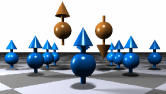
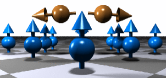
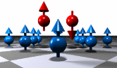
(a) (b) (c) (d)

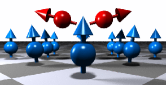
Figure 6: Most stable configurations of Cr/Mn dimer obtained with (a/c) the collinear KKR method and (b/c) the non-collinear KKR method. The rotation angle with respect to the $z$ axis is equal to 94.2^∘/72.6^∘. While the non-collinear state is the ground state for Mn-dimer it is only a local minimum for Cr-dimer. Atoms in blue correspond to the Ni substrate. Adapted with permission from Ref.lounis05 .

The starting, frustrated collinear configuration is the ferrimagnetic (FI) state, to be compared to the non-collinear configurations for Cr and Mn dimers on Ni(001). When we allow for a rotation of the magnetic moments, non-collinear solutions are obtained for the Cr- and Mn-dimer/Ni(001) systems. Fig. 6(a) represents the collinear magnetic ground state of the Cr system. As one expects from the adatom picture, both adatoms forming the dimer tend to couple AF to the substrate but due to their half filled d band they also tend to couple AF to each other.

Thus there is a competition between the interatomic coupling within the dimer, which drives it to a FI state, and the exchange interaction with the substrate, which drives the moments of both atoms in the same direction: AF for Cr and FM for Mn. As discussed in the previous section, the magnetic exchange interaction (MEI) to the substrate is relatively weak for Cr and Mn. Thus, the intra–dimer MEI is stronger than the MEI with the substrate, and in the collinear approximation the ground state is found FI. Removing the collinear constraint, a compromise can be found such that both adatom moments are oriented almost to each other and at the same time (for Cr) slightly AF to the substrate. This is shown in Fig. 6(b): the Cr adatom moments are aligned antiparallel to each other and basically perpendicular to the substrate moments. However, the weak AF interaction with the substrate causes a slight tilting, leading to an angle of 94.2^∘ with respect to the surface normal, instead of 90^∘. We also observe a very small tilting ($\approx 0.3^{\circ}$) of the magnetic moments of the four outer Ni atoms neighboring the Cr dimer (the two inner Ni atoms do not tilt for symmetry reasons).

Despite the above considerations, the collinear FI state (Fig. 6(a)) is also a self-consistent solution of the Kohn-Sham equations, even if the collinear constraint is removed. Total energy calculations are needed in order to determine if the non-collinear state (NC) is the true ground state, or if it represents a local minimum of energy with the collinear result representing the true ground state. After performing such calculations we find that the ground state is actually collinear with an energy difference of $\Delta E_{\mathrm{NC}-\mathrm{FI}}=40$ meV to the non-collinear state. This delicate balance cannot be captured by the Heisenberg model with fitted exchange interactions, but requires self-consistent density-functional calculations.

The result is different for a Mn dimer. Fig. 6(c) and (d) show the collinear and the non-collinear solutions. The dimer atoms couple strongly antiferromagnetically to each other but, just as for the single Mn adatoms, they also couple (weakly) ferromagnetically to the substrate. Both adatom moments, while aligned AF with respect to each other, are tilted in the direction of the substrate magnetization. With a rotation angle of $\approx 72.6^{\circ}$, the deviation from the $90^{\circ}$ configuration is rather large. Also the Ni moments are tilted by $7.4^{\circ}$. Finally total-energy calculations show that for the Mn-dimer the non-collinear solution is the ground state (total energy calculations yield $\Delta E_{\mathrm{NC}-\mathrm{FI}}=-13$ meV).

In both cases (Cr and Mn dimers) the frustrated collinear solution is asymmetric, while the non-collinear ground state restores the twofold symmetry of the system. The differences in energy between the FI and the non-collinear solutions are small and can be altered either by using a different type of exchange and correlation functional such as GGA or LSDA$+U$, or after relaxing the atoms. We note, however, that in a test calculation we found the Cr single-adatom relaxation to be small (3.23 % inward with respect to the interlayer distance), and thus we believe that the relaxation cannot affect the exchange interaction considerably.

As a cross-check, it is interesting to compare these non-collinear ab-initio results to model calculations based on the previously defined Heisenberg model 1 with the exchange parameters fitted to the total energy results. Taking into account only nearest-neighbor interactions and neglecting the rotation of Ni moments, we rewrite the Hamiltonian for the dimer in terms of the tilting angles $\theta_{1}$ and $\theta_{2}$ of the two Cr (or Mn) atoms (the azimuthal angles $\phi$ do not enter the expression because of symmetry reasons):

$${H}=-J_{\mathrm{Cr-Cr}}\cos(\theta_{1}-\theta_{2})-4J_{\mathrm{Cr-Ni}}(\cos\theta_{1}+\cos\theta_{2})+\mathrm{const}.$$ (11)

The interatomic exchange constants $J_{\mathrm{Cr-Ni}}$, $J_{\mathrm{Mn-Ni}}$, $J_{\mathrm{Mn-Mn}}$ and $J_{\mathrm{Cr-Cr}}$ are evaluated via a fit to the total energy obtained from collinear LSDA calculations of the FM, AF, and FI configurations.

We note the two extreme cases arising from this Heisenberg Hamiltonian: (i) $|J_{\mathrm{Cr-Ni}}|\gg|J_{\mathrm{Cr-Cr}}|$ leads to the stabilization of the collinear FM or AF configuration (adatom-like behavior) and (ii) $|J_{\mathrm{Cr-Ni}}|\ll|J_{\mathrm{Cr-Cr}}|$ leads to antiferromagnetic coupling within the dimer if $J_{\mathrm{Cr-Cr}}<0$. Within the Heisenberg model the FI solution and the non-collinear solution with $\theta=90^{\circ}$ have the same energy.

Table 1 summarizes the estimated exchange parameters.

$J_{ij}$ (meV)	$J_{\mathrm{Cr-Ni}}$	$J_{\mathrm{Cr-Cr}}$	$J_{\mathrm{Mn-Ni}}$	$J_{\mathrm{Mn-Mn}}$
(a)	$-1.3$	$-189.1$	$13.0$	$-138.2$
(b)	$-11.6$	$-221.3$	$27.0$	$-140.2$

Table 1: Values of magnetic exchange parameters $J_{ij}$ for Cr and Mn dimers on Ni(001), and obtained by the Lichtenstein formula lichtenstein (a) and extracted from collinear first-principles total energy calculations (b) ($J_{\mathrm{Cr-Ni}}$ and $J_{\mathrm{Mn-Ni}}$ are averaged over the different Ni nearest neighbors of the dimer atoms). Positive $J_{ij}$ correspond to ferromagnetic interactions, negative $J_{ij}$ to antiferromagnetic ones. Adapted with permission from Ref. lounis05

.

It is striking that the strong antiferromagnetic Cr-Cr and Mn-Mn interaction for the dimer (nearest neighbors) are more than an order of magnitude larger than the exchange interactions with the substrate, and responsible for the stabilization of the non-collinear states shown in Fig. 6. The exchange constants $J_{ij}$ fitted to total energy results can be compared to the ones obtained by starting from the FI state and using the Lichtenstein formula lichtenstein , having in mind also its restriction to low-angle rotations bruno ; lichtenstein2 ; lounis_jij . This rests on the force theorem, and yields the exchange constants corresponding to an infinitesimal rotation of the moments. The results of the two methods agree best for the Mn-Mn interaction, and reasonably well for the Cr-Cr interaction, but not for Mn-Ni and Cr-Ni. This is expected, since a rotation causes a significant change in the magnitude of the Ni moments, so that the force theorem is not applicable any more.

With the parameters from Table 1 one can also recalculate the non-collinear structure of the ground state. The agreement with the ab-initio results is quite reasonable. For the Cr dimer, one finds a slightly smaller tilting, i.e. 96^∘ instead of 94.2^∘, while for the Mn dimer the angle is 67.3^∘ instead of 70.6^∘.

The differences in energy calculated within this simple model suggest that the Cr-dimer has a non-collinear ground state ($\Delta E_{\mathrm{NC}-\mathrm{FI}}=-9.7$ meV) as well as the Mn-dimer ($\Delta E_{\mathrm{NC}-\mathrm{FI}}=-42$ meV). The discrepancy obtained for the case of Cr-dimer (the LSDA calculation gives the collinear FI ground state) can be attributed to the restrictions of the Heisenberg model. For instance, for the FI and non-collinear configurations, the Cr moments are slightly different, and also the reduction of the Ni moments as a function of the rotation angle cannot be described by the Heisenberg model, where the absolute values of the moments are assumed to be constant. Within the Heisenberg model, the FI solution (with $\theta_{1}=0^{\circ}$ and $\theta_{2}=180^{\circ}$) is degenerate with the non-collinear solution ($\theta_{1,2}=90^{\circ}$ with AF coupling within the dimer).

To evaluate the effect of change in coordination and hybridization, we have undertaken a study of inatom dimers (i.e., embedded in the surface layer), where we found that the ground state is of FI type for both Cr and Mn systems. It is interesting to note that recent simulations on Mn dimers deposited on Ni(001) surface were presented in Ref. stepanyuk considering the impact of an external electric field. It was shown that depending on the magnitude of the field, switching of the nature of magnetic ground state can be achieved.

On the fcc Fe_3ML/Cu(001) surface, the magnetic coupling between the surface atoms and the adatoms is expected to be stronger than on Ni(001) surface. Because of the AF coupling preference of the single Mn adatom to the substrate, the Mn–dimer is characterized by a non-collinear magnetic solution where the two moments are slightly tilted AF to the substrate ($\theta=115^{\circ}$). The Cr-dimer is, however, FI and no NC solution was found. The reason is the very strong AF coupling of the single Cr adatom to the Fe surface moments, that cannot be overcome by the MEI between the adatom and the substrate moments. In order to explain this we use the Heisenberg model, Eq. (11), to calculate the angle $\theta_{1}=\theta_{2}=\theta/2$ defining the non-collinear solution:

$$\cos(\theta)=-2\frac{J_{\mathrm{Cr-Fe}}}{J_{\mathrm{Cr-Cr}}}\ \mathrm{for}\ 2J_{\mathrm{Cr-Fe}}<J_{\mathrm{Cr-Cr}}$$ (12)

If $2|{J_{\mathrm{Cr-Fe}}|>|J_{\mathrm{Cr-Cr}}}|$, the angle is not defined and the solution is collinear. This is clearly realized in the present case: $2|{J_{\mathrm{Cr-Fe}}}|=2\times 80.8>|{J_{\mathrm{Cr-Cr}}}|=78$ meV. Note that the Cr-Fe coupling constants are considerably smaller than for the single adatom.

On Ni(111) surface, the magnetic behavior for the Cr and Mn dimers is similar to the behavior on Ni(001) surface with the difference of a reduction of the adatom-substrate MEI due to the lower coordination on Ni(111). This leads once more to a FI ground state for Cr-dimer whereas non-collinearity is a metastable state for Mn-dimer. Energetically, this state characterized with a rotation angle of $\theta=79^{\circ}$ is slightly higher, by 4.4 meV/adatom, than the energy of the FI solution.

V Chains

Now that we found the presence of both collinear and non-collinear states in dimers, it is reasonable to ask what happens in larger systems, such as antiferromagnetic clusters or chains. Within the Heisenberg model, the infinite antiferromagnetic chain deposited on a ferromagnetic surface is predicted to be non-collinear with atomic moments tilted in a similar fashion as the dimer moments at the condition that dimer is non-collinear lounis_prl . But what is the ground state of finite-length chains? For a preliminary answer one can employ again the classical Heisenberg Hamiltonian that we rewrite as follows:

$$H = -J_{1}\sum_{i=1}^{N-1}\cos(\theta_{i}-\theta_{i+1})-J_{2}\sum_{i=1}^{N}\cos(\theta_{i}).$$ (13)

$N$ is the number of atoms in the chain and $\theta$ is the rotation angle of the chain atom moment with respect to the magnetization of the surface. $J_{1}$($<0$) stands for an (antiferromagnetic) exchange interaction between two neighboring chain atoms at sites $i$ and $i\pm 1$ in the chain, while $J_{2}$ is the interaction between a given chain atom and the substrate.

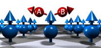
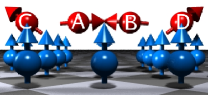
(a) (b) (c)

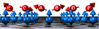
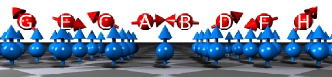
(d) (e)

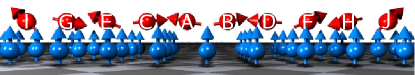
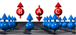
(f) (g)

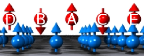
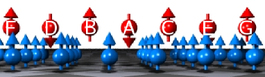
(h) (i)

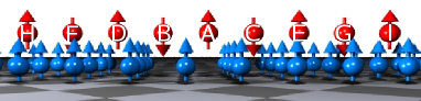
Figure 7: Magnetic ground configurations of the Mn nanochains on Ni(001) calculated with the KKR method. The nanochains with even number of Mn atoms (2, 4, 6, 8, 10) prefer a non-collinear ground state, the odd ones a collinear one. Atoms in blue correspond to the Ni substrate. Adapted with permission from Ref.lounis_prl .

Table 2: Ab initio results for even-numbered nanochains: size and angle of the magnetic moments as well as total energy differences between the NC and FI solutions. In every pair of chain atoms connected by a “-” sign, the azimuthal angles $\phi$ are equal to 0^∘-180^∘, while the magnetic moments and rotation angles $\theta$ are the same. Adapted with permission from Ref. lounis_prl

Length	$E_{\mathrm{NC}}-E_{\mathrm{FI}}$	Adatom	$\theta$(∘)	$M$ ($\mu_{B}$)
(adatoms)	(meV/adatom)
2	$-$11.16	A-B	73	3.71
4	$-$8.48	A-B,C-D	87, 54	3.55, 3.72
6	$-$7.82	A-B, C-D,	70, 104,	3.46, 3.52,
		E-F	45	3.67
8	$-$5.46	A-B, C-D,	84, 65,	3.47, 3.46,
		E-F, G-H	106, 44,	3.52, 3.66
10	$-$3.53	A-B, C-D,	78, 85,	3.47, 3.47
		E-F, G-H,	67, 102,	3.46, 3.52
		I-J	48	3.67

As an example, Mn-chains on Ni(001) surfaces are discussed; the obtained results are rather general  lounis_prl . For the dimer-case, the energy of the FI solution depends only on $J_{1}$ ($E_{\mathrm{FI}}=J_{1}$), because the contributions $J_{2}$ of both adatoms cancel out due to their antiparallel alignment. On the other hand, the energy of the NC solution (Fig. 7(a)) depends also on the magnetic interaction with the substrate in terms of $J_{2}$ ($E_{\mathrm{NC}}=-J_{1}\cos(2\theta)-2J_{2}\cos(\theta)$). For three Mn adatoms (Fig. 7(f)), we find the FI solution to be the ground state. Contrary to the dimer, the energy of the collinear solution of the trimer depends on $J_{2}$ ($E_{\mathrm{FI}}=2J_{1}-J_{2}$) due to the additional third adatom, which in fact allows the FI solution to be the ground state.

One sees here the premise of an odd-even effect on the nature of the magnetic ground state. On this basis one can conjecture that chains with even number of atoms would behave similarly to the dimer, because an additional energy with the substrate proportional to $J_{2}$ can be gained in the NC state by the small tilting off the $90^{\circ}$ angle shown in Fig. 7(a), while odd-numbered chains would behave similarly to the trimer. They can always gain energy in the collinear state due to one $J_{2}$ interaction term which does not cancel out.

Investigating the longer nanochains with even number of atoms shows that their ground state is always NC. Examples, calculated with the KKR method, are presented in Fig. 7(b)-(c)-(d)-(e) and in Table 2. In a first approximation, the magnetic moments are always in the plane perpendicular to the substrate magnetization keeping the magnetic picture seen for the dimer almost unchanged. Moreover, the neighboring magnetic moments are coupled almost AF. The atoms at both ends of the chains are closest to a FM orientation to the substrate (see Table 2). The two central chain atoms A-B (see Fig. 7 for the notation) are the ones which keep their rotation angles almost unaltered with respect to the dimer. The angle $\theta$ oscillates between 70^∘ obtained for the chain with 6 atoms up to 87^∘ obtained for the chain with 4 atoms. Note that the angle between two successive moments is about 150^∘, similar to the dimer result.

The considered odd-numbered nanochains are characterized by a FI ground state in which the majority of atoms are coupled FM to the surface. The total energy differences to the lowest lying metastable, i.e. NC state, first increases with respect to the length of the chain (see Table 3) up to a maximum for a chain with 7 atoms (10.5 meV/adatom) followed by a decrease for longer chains. This behavior is the property of the metastable NC state and arises from a competition between the edge and inner atoms of the chain. Edge atoms in odd chains favor collinear moment alignment to the substrate. For short chains, trimer and 5 atoms chains, they dominate the total magnetic behavior permitting only a slight tilting of the moments away from the FI state. For longer chains, however, the inner atoms experience basically the same local environment as the atoms in even chains resulting in similar moment orientations.

When increasing the length of the chains, both kinds of chains should converge to the same magnetic ground state since the even-odd parity is expected to be obsolete for infinite systems. Within the DFT framework, the investigation of longer chains is computationally very demanding. Thus, the Heisenberg model is used to investigate this magnetic transition.

Table 3: Ab initio results for odd-numbered nanochains: size of the magnetic moments and total energy differences between the NC and FI state. Atoms connected by a hyphen have the same magnetic moment.

Length	Adatom	$M$ ($\mu_{B}$)	$E_{\mathrm{NC}}-E_{\mathrm{FI}}$
(adatoms)		for FI	(meV/adatom)
3	A, B-C	$-$3.78, 3.65	8.85
5	A, B-C, D-E	3.43, $-$3.56, 3.64	9.52
7	A, B-C, D-E,	$-$3.54, 3.43, $-$3.56	10.48
	F-G	3.64
9	A, B-C, D-E,	3.43, $-$3.54, 3.43	9.29
	F-G, H-I	$-$3.56, 3.64
11	A, …, K-L	$-$3.59, …, 3.67	6.49

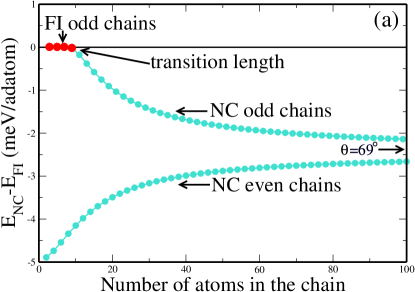
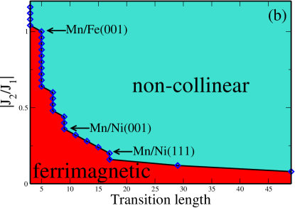
Figure 8: (a) Energy differences obtained from the Heisenberg model between the NC and the FI configuration for different lengths of Mn chains on Ni(001). The parameters used were $J_{1}=-138$ meV and $J_{2}=52$ meV. (b) Magnetic phase diagram of the odd chains showing the effect of the ratio ${J_{2}}/{J_{1}}$ on the transition lengths. If the length of the chains is smaller than the transition length, the FI configuration is the ground state. Adapted with permission from Ref.lounis_prl .

We discuss now the Heisenberg Model results. Two different approaches are used to solve Eq.13. In the first approach we allow the rotation angle $\theta_{i}$ to vary from site to site in the chain and in the second we consider a constant absolute value of $\theta$ at each site. The first, the inhomogeneous approach, requires an iterative numerical scheme while the second, the homogeneous one, leads to a simple analytical form. In Fig. 8(a), the energy difference between the NC and FI states determined by the first approach is plotted versus the length of Mn-nanochains. Negative values refer to a NC ground state. The model reproduces the DFT results showing that the even chains have always a NC ground state. Within this model, the ground state for odd chains changes from FI to NC when the number of atoms exceeds a transition length of 9 atoms which is smaller than what predicted from DFT. Moreover, even beyond this length, we notice an oscillatory behavior of the energy differences and the magnetic structure when going from the odd- to even-numbered chains. This behavior is easier to understand when considering the homogeneous ansatz, which leads to a somewhat larger transition length (19 atoms) for the odd chains. In this case, the energy difference per chain atom is given by $\Delta E_{\mathrm{NC-FI}}=\frac{NJ_{2}^{2}}{8(N-1)J_{1}}+P(N)\frac{|J_{2}|}{N}$, with $P(N)$, a parity function, equals 0 if $N$ is even, and 1 if $N$ is odd. Since the first term of $\Delta E_{\mathrm{NC-FI}}$ is negative for all lengths ($J_{1}<0$), NC is the ground state for all even-chains. The second term on the other hand is positive and provides for finite lengths an energy counterbalance allowing FI as the lowest energy solution. As this term decreases as $N^{-1}$, a cross-over to non-collinearity is expected for $N\approx 8|J_{1}|/|J_{2}|$, as found in Fig. 8(a). Moreover, we notice that for big values of $N$, $\Delta E_{\mathrm{NC-FI}}$ converges to a constant, ${J_{2}^{2}}/{(8J_{1}})$, which is confirmed by the convergence of the two curves in Fig. 8(a) towards the same NC state with $\theta_{\mathrm{NC}}=69^{\circ}$: if the chains are infinite the parity induced differences vanish.

The next point is the discussion of the general behavior of the transition length for odd chains. Using the inhomogeneous ansatz, we determine for each set of parameters ($J_{1}$, $J_{2}$) the corresponding transition length which leads to the phase diagram shown in Fig. 8(b). The obtained curve seems to decay roughly as $N^{-1}$. On one hand, small exchange-interaction ratios lead to very long transition lengths. This means that odd-even effects are expected to last for very long chains which can be easily observed experimentally. On the other hand, large values of $J_{2}$ compared to $J_{1}$ lead to very small transition lengths. The obtained phase diagram is interesting and can be used to predict the behavior as well as the transition lengths for other kinds of AF chains deposited on FM substrates. This model predicts for example a transition length of 5 atoms for Mn/Fe(001) while Mn/Ni(111) is characterized by a value of 17 atoms. Certainly, this transition length is subject to modifications depending on the accuracy of the exchange interactions, spin-orbit coupling and geometrical relaxations. Furthermore, we point out that the angles $\theta$ obtained by the model are in good agreement with our DFT calculations, meaning that the model reliably describes the very-long chains. In addition, it is interesting to note that a recent experimental as well as theoretical work revealed a similar NC behavior for a full-monolayer of Mn deposited on a bcc Fe(001) surface baroni . We note that recent simulations petrilli on Mn nanowires on bcc Fe(001) did not show the even-odd behavior since the magnetic exchange interactions among the nearest neighboring Mn adatoms were antiferromagnetic but smaller then the ferromagnetic magnetic exchange interaction with the substrate. Thus a non-collinear state is not expected in this situation (Eq. (12) is not fulfilled). However, interesting sinusoidal modulation of the magnetization is obtained with a period corresponding to the length of the Mn nanowires.

Recently, spin-polarized STM experiments on Mn nanowires deposited on Ni(110) combined with DFT calculations verified the existence of an even-odd effect in the magnetic ground states wulfhekel . Similar to Ni(001) substrate, the even-numbered wires are non-collinear while the odd-numbered ones are collinear. Interestingly, the ferrimagnetic contrast was observed experimentally for the trimer, but for the dimer and tetramer no signal was observed. This is reasonable since if there is no spin-orbit coupling the tilted moments of Mn atoms can rotate freely around the magnetization of the substrate. Thus, there is no possibility to observe a contrast from the components of the adatoms magnetic moments perpendicular to the magnetization of the surface while the parallel components are difficult to distinguish. In Ref. wulfhekel , an additional proposal is made for the fluctuations of the magnetization using zero-point energy motion for even-numbered chains. Indeed, although a barrier, induced by the spin-orbit interaction, exists between equivalent orientations of the magnetic moments, the strength of the fluctuations, evaluated within the Landau-Lifschitz-Gilbert formalism, is larger than the barrier. More details can be found in Ref. wulfhekel .

VI Compact clusters

VI.1 Fcc(001) surfaces

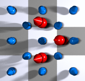
(a) (b)

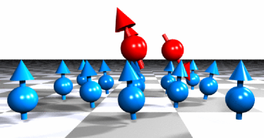
Figure 9: Non-collinear state of the Mn trimer on Ni(001) surface. Side view (a) and front view (b) are shown. This represents a local minimum in energy, with the collinear state being the ground state (see text). Atoms in blue correspond to the Ni substrate. Reprinted with permission from Ref. lounis05 . Copyright 2005 by the American Physical Society.

So far we have examined a simple one-dimensional geometry of the magnetic nanostructure, which can be stabilized at low enough temperatures. One expects, however, more compact structures to occur, where the increased coordination will favor a reduction of the cohesive energy. For example, instead of the aforementioned linear trimer, an isosceles rectangular triangle would occur on an fcc(001) surface (see Fig. 9).

In such a triangle on Ni(001), it is expected, and verified by total-energy calculations, to find the $\downarrow\uparrow\downarrow$ configuration as the collinear magnetic ground state for Cr and the $\uparrow\downarrow\uparrow$ for the Mn trimer ($\uparrow$ means an atomic moment parallel to the substrate magnetization, $\downarrow$ means antiparallel; the middle arrow represents the direction of the atomic moment at the right-angle corner of the triangle).

Allowing free rotation of the magnetic moments leads to no change for the Cr trimer $\downarrow\uparrow\downarrow$—the state remains collinear (within numerical accuracy). On the other hand, for the Mn trimer a non-collinear solution is found (Fig. 9) with the nearest neighbors almost antiferromagnetic to each other, but with a collective tilting angle with respect to the substrate. This tilting angle is induced by the ferromagnetic MEI between the central Mn atom with the substrate, competing with the antiferromagnetic MEI with its two companions. The top view of the surface shows that the in-plane components of the magnetic moments are collinear.

The tilting is somewhat smaller ($21.7^{\circ}$) for the two Mn atoms with moments up than for the Mn atom with moment down ($28.5^{\circ}$). Also the neighboring Ni–surface atoms experience small tilting, with varying angles around $4^{\circ}-10^{\circ}$. From the energy point of view, the ground state is collinear, $\uparrow\downarrow\uparrow$, with an energy difference of $\Delta E_{\mathrm{NC}-\uparrow\downarrow\uparrow}=23$ meV with respect to the local-minimum, non-collinear solution.

One should note that the moments of the two first neighboring impurities are almost compensated in the FI solution. The third moment determines the total interaction between the substrate and the trimer which has then a net moment coming mainly from the additional impurity. This interaction is identical to the single adatom (or inatom) type of coupling.

On Fe_3ML/Cu(001) surface, the nature and type of non-collinear structure of the trimer do not change much compared to what is obtained on Ni(001) surface. The only difference is that, here, the non-collinear solution is the ground state for the compact Cr- and Mn-trimer. The addition of a third adatom to the system forces a rotation of the moments. The two second-neighboring Cr/Mn impurities B and C (see Fig. 10(a)) have a moment tilted towards the surface by an angle of 156^∘/170^∘ (24^∘/10^∘ from the AF coupling) and adatom A moment is tilted up/down with an angle of 77^∘/20^∘. As can be noticed, the moment of the central adatom rotates by approximately twice the rotation angle of the moments of the outer adatoms. This is explained by the fact that the central magnetic moment experiences twice the AF exchange coupling from its two first neighboring atoms.

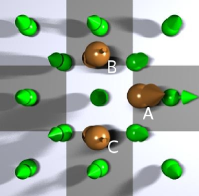
(a) (b)

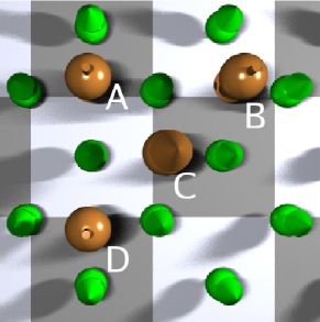
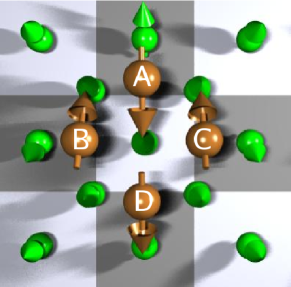
(c) (d)

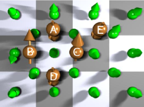
Figure 10: Front views of complex magnetic states of Cr ad-clusters on Fe_3ML/Cu(001) surface: (i) the trimer is shown in (a), (ii) the T-shape tetramer (tetramer 2) is presented in (b), (iii) the tetramer 1 is depicted in (c) and finally pentamer 1 is shown in (d). Unlabeled atoms (in green) correspond to the Fe substrate. Reprinted with permission from Ref.lounis08 . Copyright 2008 by the IOPscience.

We extended our study to bigger clusters, namely tetramers and pentamer. Two types of tetramers were considered: tetramer 1 is the most compact and forms a square (Fig. 10(c)), while tetramer 2 has a T-like shape (Fig. 10(b)). The ground state of Cr–tetramer 1 is non-collinear (Fig. 10(c)) with a magnetic moment of 2.5 $\mu_{B}$ carried by each impurity. One notices that the neighboring adatoms are almost AF coupled to each other(the azimuthal angle $\phi$ is either equal to 0⁰ or to 180⁰) with all moments rotated by the angle $\theta$ = 111^∘. Contrary to Cr, Mn–tetramer 1 has a collinear FI magnetic ground state with a total energy slightly lower (2.3 meV/adatom) than the energy of the non-collinear metastable solution. The latter is similar to the solution depicted in Fig. 10(c) but with moments slightly tilted upwards.

For Cr–tetramer 2 (see Fig. 10(b)) we obtained several collinear magnetic configurations. The most favorable one is characterized by an AF coupling of the three corner atoms with the substrate. The moment of adatom C, surrounded by the remaining Cr impurities, is then forced to orient FM to the substrate. When we allow for the direction of the magnetic moment to relax, we get a non-collinear solution having a similar picture, energetically close to the collinear one ($\Delta E_{\mathrm{col}-\mathrm{NC}}=2.3$ meV/adatom). Adatom C has now a moment somewhat tilted by 13^∘ ($\mu=$ 2.31 $\mu_{B}$) whereas adatom A has a moment tilted in the opposite direction by 172^∘ ($\mu=$ 2.85 $\mu_{B}$). Adatoms B and D have a moment of 2.87 $\mu_{B}$ with an angle of 176^∘. We note that tetramer 1 with a higher number of nearest-neighboring bonds (four instead of three for tetramer 2) is the most stable one ($\Delta E_{\mathrm{tet2}-\mathrm{tet1}}=14.5$ meV/adatom) with the non-collinear solution shown in Fig. 10(c).

To study the pentamers, we have chosen two structural configurations: pentamer 1 (Fig. 10(d)) with the highest number (five) of first neighboring adatom bonds (NAB) and pentamer 2 which is more compact has only four NAB. The latter one is obtained by extending the tetramer of Fig. 10(b) symmetrically with an additional adatom forming an X-shaped cluster. The pentamer 1 consists on a tetramer of type 1 plus an adatom (E) and is characterized by a non-collinear ground state. Let us understand the solution obtained in this case by starting from tetramer 1 (Fig. 10(d)), which is characterized by a non-collinear almost in-plane magnetic configuration. As we have seen, a single adatom is strongly AF coupled to the substrate. When attached to the tetramer it affects primarily the first neighboring impurity (adatom C) by tilting the magnetic moment from 111^∘ to 46^∘. Adatom E is also affected by this perturbation and experiences a tilting of its moment from 180^∘ to 164^∘. As a second effect, the second neighboring adatom, A, is also affected and suffers a moment rotation from 111^∘ to 138^∘. The AF coupling between first neighboring adatoms is always stable, thus adatom D has also a moment rotated opposite to the magnetization direction of the substrate with an angle of 155^∘ ($\mu=$  2.48 $\mu_{B}$). As adatom B tends to couple AF to its neighboring Cr adatoms, its magnetic moment tilts into the positive direction with an angle of 85^∘.

On the other hand, pentamer 2 is characterized by a non-collinear solution which is very close to the collinear one: the outer adatoms are AF coupled to the surface magnetization while the moment of the central adatom is forced to be oriented FM to the substrate. Surprisingly, this ad-cluster which has less first NAB (four instead of five) has a lower energy compared to pentamer 1. Here, energy difference between the two structural configurations is about 37 meV/adatom. The strength of the second NAB seem to be as important or stronger than the first NAB.

VI.1.1 Experiment

It is interesting to compare the aforementioned theoretical results to measurements determined using X-ray magnetic circular dichroism (XMCD). This type of experiments allows to determine the of spin or moment, $M_{z}$, per number of d-holes, $n_{d}$. The experiments were performed by the group of Wurth lounis08 on size-selected Cr ad-clusters deposited by soft-landing techniques on Fe_3ML/Cu(001). The nature of the experiment is such that a large surface area is sampled, and also only the size of the clusters is known, but not the shape. Therefore the experimental result is a statistical average over a number of (unknown) cluster shapes. After applying XMCD sum rules Laan99 , the Hamburg group of Wurth lounis08 arrived at the result shown in Fig. 11.

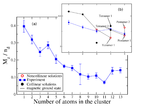
Figure 11: Spin moment per number of d-holes per atom versus cluster size for Cr clusters on a Fe_3ML/Cu(001) ferromagnetic substrate. Panel (a) shows experimental results for cluster-sizes up to 13 adatoms while panel (b) gives the comparison with ab initio results for cluster-sizes up to 5 adatoms. Blue squares describe the experimental values, black diamonds show represent collinear configurations, red circles correspond to non-collinear configurations and a black line connects the ratios obtained in the magnetic ground states. Reprinted with permission from Ref.lounis08 . Copyright 2008 by the IOPscience.

One notices the strong decrease of $M_{z}/n_{d}$ with increasing cluster size which is due to the appearance of antiferromagnetic or non-collinear structures as calculated by theory. The qualitative and quantitative trends observed in the experimental results agree well with the theoretical results (Fig. 11(b)) for Cr-atoms to Cr-pentamers. Although the theoretical values for Cr-atoms and dimers lie somewhat higher than the experimental values (including error bars) the agreement can still be judged to be very good in view of the remaining experimental uncertainties. Even details as the increase of spin magnetic moment from trimer to tetramer can be addressed. In order to understand the peak formed for the tetramer we compare in Fig. 11.(b) the ratio $M_{z}/n_{d}$ between the moment along the $z$-direction (defined by the magnetization of the substrate) and number of holes per atom obtained by theory for the different geometrical and spin structures. Black circles show the ratio calculated by taking into account the collinear solutions and the red ones show the ratio calculated from the non-collinear solutions. The black line connects the ratio obtained in the magnetic ground states. The non-collinear tetramer 1 has a much lower value than what was seen experimentally whereas the collinear tetramer 1 and tetramer 2 give a better description of the kink seen experimentally. With regards to the small energy difference ($\Delta E=14.5V$ meV) between the two tetramers considered, one could interpret the experimental value as resulting from an average of non-collinear tetramers 1, collinear and non-collinear tetramer 2. We believe that this explains why the tetramer ratio value is higher than the one obtained for a trimer. The trimer and the pentamers are clearly well described by the theory and fit to the experimental measurements.

VI.2 Fcc(111) surfaces

Before discussing the complex spin structures induced by a magnetic surface with triangular symmetry, it is instructive to look at the simpler cases of non-magnetic substrates.

VI.2.1 Non-magnetic surfaces

Using the RS-LMTO-ASA method, Bergman and co-workers bergman found that the ground state for the most compact Cr and Mn trimers is the Neel state with a rotation angle of 120^∘ between the magnetic moments (Fig. 12(a)). Such a non-collinear structures was also reported from calculations on Cr clusters, with the same geometry, supported on Au(111) surface gotsis ; bergman_gold .

In Figs. 12(b) and 12(c) more interesting structures are explored bergman . First six Mn atoms forming a hexagonal ring structure were studied [Fig 12(b)]. The antiferromagnetic nearest neighbor interaction causes a magnetic order where every second atom has its magnetic moment pointing up and every other has a moment pointing down, and the magnetic order is collinear. However, for the cluster with one extra atom in the center of the hexagonal ring [Fig. 12(c)] frustration occurs leading to a different magnetic order with a non-collinear component. The atoms at the edge of the cluster have a canted anti-ferromagnetic profile, with a net moment pointing antiparallel to the magnetization direction of the atom in the center of the cluster. The magnetic moment of the central atom is almost perpendicular ($\sim$ 100 ^∘) to the atoms at the edge of the cluster and with a magnetic moment of 2.7 $\mu_{B}$. The edge atoms have a magnetic moment of 4 $\mu_{B}$ each that has an angle of $\sim$ 165^∘ to neighboring edge atoms and is parallel to its second nearest neighbors. Interestingly, the non-collinear behavior does not occur for a Cr sextamer whereas the heptamer is non-collinear.

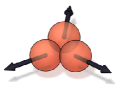
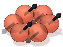
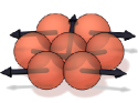
Figure 12: The magnetic ordering for Mn clusters on a Cu(111) surface according to calculations by Bergman et al. bergman (Adapted with permission - Copyright American Physical Society (2006)).

On the Au(111) surface, Antal and coworkers antal investigated the magnetic behavior of Cr ad-clusters using a the fully-relativistic KKR method. They also found the equilateral trimer to exhibit a frustrated 120^∘ Néel type of ground state with interestingly a small out-of-plane component of the magnetization that is induced by relativistic effects. In the cases of a linear chain and an isosceles trimer, collinear antiferromagnetic ground states are obtained with the magnetization lying parallel to the surface.

An interesting investigation was carried out by Ribeiro et al. klautau_pt for Mn corrals deposited on Pt(111) surface. In the considered structures, the coupling between nearest neighbors Mn adatoms is of antiferromagnetic nature and the magnetic ground state is found to be collinear and ferrimagnetic. But as soon as an additional Mn adatom is attached to the corral, non-collinear orientations of the magnetic moments are induced along the whole corrals similarly to the simulations presented in Ref. nikos .

VI.2.2 Magnetic surface: Ni(111)

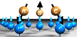
(a) (b)

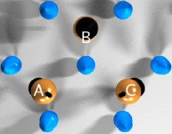
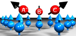
(c) (d)

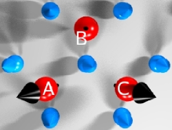
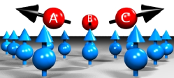
(e) (f)

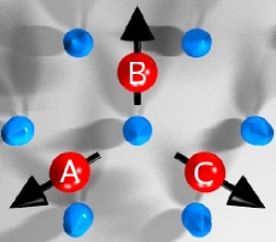
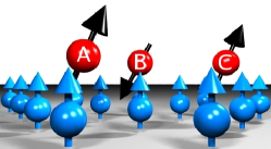
(g) (h)

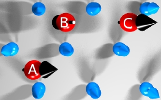
Figure 13: Side view (a) and top view (b) for the most stable configuration of Cr compact trimer on Ni(111); this corresponds also to the NC1 configuration of the Mn compact trimer. (c) and (d) represent the side view and top view of the ground state (NC2) of Mn compact trimer on Ni(111) while (e) and (f) depict an almost degenerate state (NC3) of the same Mn trimer. Finally, the side view (g) and top view (h) are shown for the most stable configuration of Mn corner trimer on Ni(111). The adatoms are labeled by A, B, and C. Unlabeled atoms (in blue) correspond to the Ni substrate. Reprinted with permission from Ref.lounis07 . Copyright 2007 by the American Physical Society.

As mentioned previously, trimers in equilateral triangle geometry are, in the presence of antiferromagnetic interactions, prototypes for non-collinear magnetism, with the magnetic moments of the three atoms having an angle of 120^∘ to each other. In our case, the 120^∘ state is perturbed by the exchange interaction with the substrate, and therefore the magnetic configuration is expected to be more complicated.

Let us start with a Cr dimer (Mn dimer) that we approach by a single Cr adatom (Mn adatom). Three different types of trimers can be formed: i) the compact trimer with an equilateral shape, ii) the corner trimer with an isosceles shape and iii) the linear trimer. The adatoms are named A, B and C, as shown in Fig. 13 (see Ref. lounis07 ).

In the most compact trimer, the distance between the three adatoms is the same leading to a strong intra-cluster frustration. This is attested for the Cr case for which we had difficulties finding a collinear solution. Our striking result, as depicted in fig. 13a-b, is that the non-collinear 120^∘ configuration is conserved with a slight modification. Indeed, our self-consistent ($\theta$, $\phi)$-angles are ($2^{\circ},0^{\circ}$) for adatom B and ($126^{\circ},0^{\circ}$) for adatom A and ($122^{\circ},180^{\circ}$) for adatom C. The angle between B and A is equal to the angle between B and C (124^∘) while the angle between A and C is 112^∘. The small variation from the prototypical 120^∘ configuration is due to the additional exchange interaction with Ni atoms of the surface. The coupling with the substrate leads thus to a deviation from the prototype 120^∘ state, with an additional rotation of $2^{\circ}$ for the FM adatom and of 4^∘ for the two other adatoms. In the picture of the 120^∘-state in a non-magnetic substrate [e.g., Fig. 12(a)], the moments are usually shown as if they were parallel to the surface. However, any rotation is allowed (if spin-orbit coupling is neglected), as long as it is the same for all moments so that their directions relative to each other are the same. Here the situation is different: the substrate magnetization forces a particular absolute choice of directions, while the relative angle between the trimer moments is not changed much.

For the compact Mn trimer, three non-collinear configurations were obtained: As in the case of the compact Cr trimer, the free Mn trimer must be in a 120^∘ configuration. Nevertheless, the magnetism of the substrate changes this coupling taking into account the single adatom behavior: Mn adatoms prefer a FM coupling to the substrate and an AF coupling with their neighboring Mn adatom.

The first non-collinear magnetic configuration (NC1) is similar to the Cr one (Fig. 13(a)-(b)), i.e. the moment of adatom B is oriented FM (3.61 $\mu_{B}$) to the substrate moments while the moments A (3.67 $\mu_{B}$) and C (3.67 $\mu_{B}$) are rotated into the opposite direction with an angle of 114^∘ between B and A and between B and C.

The second non-collinear configuration (NC2) has the opposite magnetic picture (Fig. 13(c)-(d)) as compared to compact Cr trimer. Moments A and C are oriented FM to the substrate, with a tilting of $\theta$ = 49^∘, $\phi$ = 0^∘ for atom A and $\theta$ = 51^∘, $\phi$ = 180^∘ for atom C; each of them carries a moment of 3.62 $\mu_{B}$. The AF interaction of atom B with A and C forces it to an AF orientation with respect to the substrate, characterized by $\theta$ = 179^∘, $\phi=0$, and a moment of 3.70 $\mu_{B}$. Thus the trimer deviates from the $120^{\circ}$-configuration: the angles between A and B moments and B and C moments are about $130^{\circ}$, and the angle between A and C is about $100^{\circ}$.

In the third magnetic configuration (NC3) the three moments (3.65 $\mu_{B}$) are almost in-plane and perpendicular to the substrate magnetization (see Fig. 13(e)-(f)). They are also slightly tilted in the direction of the substrate magnetization ($\theta=86^{\circ}$) due to the weak FM interaction with the Ni surface atoms. Within this configuration, the 120^∘ angle between the adatoms is almost sustained. Total energy calculations show that the NC2 configuration is the ground state which is almost degenerate with NC1 and NC3 ($\Delta\mathrm{E}_{\mathrm{NC1}-\mathrm{NC2}}=1.3$ meV/adatom and $\Delta\mathrm{E}_{\mathrm{NC3}-\mathrm{NC2}}=5.6$ meV/adatom). Thus already at low temperatures trimers might be found in all three configurations; in fact the spin arrangement might fluctuate among these three 120^∘ configurations or among the three possible degenerate configurations corresponding to each of NC1 and NC2 states, produced by interchanging the moments of atoms A, B and C. Compared to the collinear state energy of the compact trimer, the NC2 energy is lower by 138 meV/adatom. This very high energy difference is due to frustration, even higher than breaking a bond as shown in the next paragraphs. Contrary to this, the corner trimer shows a collinear ground state because it is not frustrated.

The next step is to move adatom C and increase its distance with respect to A in order to reshape the trimer into an isosceles triangle (what we call “corner trimer” in Fig. 13(g)-(h)). By doing this, the trimer loses the frustration and is characterized, thus, by a collinear FI ground state: the moments of adatoms A and C are AF oriented to the substrate (following the AF Ni-Cr exchange), while the moment of the central adatom B is FM oriented to the substrate, following the AF Cr-Cr coupling to its two neighbors. The magnetic moments do not change much compared to the compact trimer.

While the non-collinear state is lost for the corner Cr trimer, it is present for the corner Mn trimer as a local minimum with a tiny energy difference of 4.8 meV/adatom higher than the FI ground state. This value is equivalent to a temperature of $\sim$ 56 K, meaning that at room temperature both configurations co-exist. Here FI means that the central adatom B is AF oriented to the substrate with a magnetic moment of 3.71 $\mu_{B}$, forced by its two FM companions A and C (moment of 3.83 $\mu_{B}$) which have only one first neighboring adatom and are less constrained. The total moment of the ad-cluster is also high ($3.95\mu_{B}$) compared to the compact trimer value, reaching the value of the non-interacting system (with the third atom of the trimer far away from the other two).

The FI solution is just an extrapolation of the non-collinear solution shown in Fig. 13(g)-(h) (with magnetic moments similar to the collinear ones) in which the central adatom B (3.70 $\mu_{B}$) tends to orient its moment also AF to the substrate ($\theta$ = 152^∘, $\phi$ = 0^∘) and the two other adatoms with moments of 3.83 $\mu_{B}$ tend to couple FM to the surface magnetization with the same angles ($\theta$ = 23^∘, $\phi$ = 180^∘). It is important to point out that the AF coupling between these two latter adatoms is lost by increasing the distance between them. Indeed, one sees in Fig. 13(g)-(h) that the two moments are parallel.

It is interesting to compare the total energies of the three trimers we investigated. The compact trimer has more first neighboring bonds and is expected to be the most stable trimer. The energy differences confirm this statement. Indeed the total energy of the Cr compact trimer is 119 meV/adatom lower than the total energy of the corner trimer. Similarly, the Mn compact trimer has a lower energy of 53 meV/adatom compared to the corner trimer.

(a)

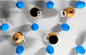
(b)

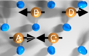
(c)

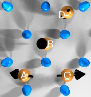
Figure 14: Top view of the collinear most stable solution (a) and the non-collinear metastable configuration (b) of compact Cr tetramer on Ni(111). In (c) is depicted the Cr tetramer-b magnetic ground state on Ni(111), which basically consists of the non-collinear trimer state of Fig.13(a) coupled antiferromagnetically to the fourth adatom. The adatoms are labeled by A, B, C, and D. Unlabeled atoms (in blue) correspond to the Ni substrate. Reprinted with permission from Ref.lounis07 . Copyright 2007 by the American Physical Society.

Finally we discuss the case of tetramers. We consider two types of tetramers, formed by adding a Cr or Mn adatom (atom D in Fig. 14) to the compact trimer. We begin with the compact tetramer (Fig. 14(a)-(b)). For both elements Cr and Mn, the FI solution is the ground state (Fig. 14(a)). The Cr tetramer, in particular, shows also a non-collinear configuration (Fig. 14(b)) as a local minimum which has, however, a slightly higher energy of $\Delta\mathrm{E}_{\mathrm{NC}-\mathrm{FI}}=1$ meV/adatom. Within this configuration the AF coupling between the adatoms is observed. However, the four moments are almost in-plane perpendicular to the substrate magnetization.

An additional manipulation consists in moving adatom D and forming a tetramer-b [Fig. 14(c)]. For such a structure, the collinear solution for the Cr tetramer is only a local minimum. In this structure, atom D has less neighboring adatoms compared to A, B, and C. In the non-collinear solution which is the magnetic ground state, the moment of adatom D (3.34 $\mu_{B}$) is almost AF oriented to the substrate ($\theta$ = 178^∘, $\phi$ = 0^∘). The remaining adatoms form a compact trimer in which the closest adatom to D, i.e. B, tends to orient its moment FM (2.45 $\mu_{B}$) to the substrate ($\theta$ = 19^∘, $\phi$ = 0^∘) while the moments of A (2.90 $\mu_{B}$) and C (2.80 $\mu_{B}$) tend to be oriented AF ($\theta_{\mathrm{A}}$ = 124^∘, $\phi_{\mathrm{A}}$ = 0^∘) and ($\theta_{\mathrm{C}}$ = 107^∘, $\phi_{\mathrm{C}}$ = 180^∘). In the (metastable) collinear solution for this tetramer, the moment of adatom B is oriented FM to the substrate while the moments of all remaining adatoms are oriented AF to the surface atoms. The total energy difference between the two configurations is equal to 49 meV/adatom. Compared to the total energy of the compact tetramer, our calculations indicate that the tetramer-b has a higher energy (109 meV/adatom).

Let us now turn to the case of the Mn tetramer-b. Also here, the non-collinear solution is the ground state while the collinear one is a local minimum. The energy difference between the two solutions is very small (2.8 meV/adatom). The moments are now rotated to the opposite direction compared to the Cr case, in order to fulfill the magnetic tendency of the single Mn adatom which is FM to the substrate. The Mn atom with less neighboring adatoms, i.e. D, has a moment of 3.84 $\mu_{B}$ rotated by ($\theta$ = 27^∘, $\phi$ = 0^∘), while its closest neighbor, atom B with a moment of 3.44 $\mu_{B}$, is forced by the neighboring companions to orient its moment AF ($\theta$ = 140^∘, $\phi$ = 180^∘). The adatoms A and C with similar magnetic moments (3.63 $\mu_{B}$) obtain a FM orientation with the following angles: ($\theta$ = 81^∘, $\phi$ = 0^∘) and ($\theta$ = 34^∘, $\phi$ = 0^∘). As in the case of Cr tetramer-b, the converged collinear solution is just the extreme extension of the non-collinear one: The “central” moment of the tetramer is forced by its FM Mn neighboring atoms to be AF to the substrate. The magnetic regime is similar to the one of Cr tetramer-b, i.e. high, with a total magnetic moment of 4.37 $\mu_{B}$. As expected, the most stable tetramer is the compact one, with an energy of 52 meV/adatom lower than tetramer b.

VII Summary and concluding remarks

In summary, we have reviewed recent work on the ab-initio investigation of complex spin-structures in ad-clusters deposited on magnetic surfaces. We have discussed prototype systems where different kinds of frustration exist: (i) frustration within the cluster and (ii) frustration arising from antiferromagnetic coupling between the adatoms in the cluster and competing magnetic interactions between the clusters and the surface atoms. We see that frustration results in non-collinear magnetic configuration on a length scale of nearest-neighbor distances. The energy scale of the directional relaxation of the magnetic moments with respect to the frustrated state can be comparable to the cohesive energy of the cluster.

In most of these cases, the present local density functional calculations give more than one energy minima, corresponding to different non-collinear states, that can be energetically very close (with differences of a few meV/atom). In these situations the system can easily fluctuate between these states. Naturally the relative energy values that were shown here can change if one corrects for the approximations that we used (neglect of spin-orbit coupling and structural relaxations, and use the local spin density approximation for the exchange-correlation energy), in particular as regards energy differences of the order of a few meV. However, the conclusion of existence of multiple almost degenerate magnetic states is expected to hold.

It is demonstrated in several occasions that the position of a single adatom within a nanostructure or the addition of an atom to a nanostructure provides a strong magnetic perturbation to the whole nano-entity. One could even envision adatoms acting as local magnetic switches, which via the local magnetic exchange field of the single adatom allow to switch the total moment on and off, and which therefore might be of interest for magnetic storage. This mechanism has been recently used experimentally to build magnetic logic gates alex_science . Thus, magnetic frustration could be useful for future nanosize information storage.

References

- (1) I. Zutic, J. Fabian, S. Das Sarma, Rev. Mod. Phys. 76, 323 (2004).
- (2) Y. Yayon, V. W. Brar, L. Senapati, et al. Phys. Rev. Lett. 99, 67202 (2007).
- (3) T. Mirkovic, M. L. Foo, A. C. Arsenault, et al. Nature Nanotechnology 2, 565 - 569 (2007).
- (4) S. Rusponi, T. Cren, N. Weiss, et al. Nature Materials 2, 546 (2003); W. Kuch, ibid. 2, 505 (2003).
- (5) J. A. Stroscio and R. J. Celotta, Science 306, 242 (2004).
- (6) J. T. Lau, A. Föhlisch, R. Nietubyć, et al. Phys. Rev. Lett. 89, 57201 (2002).
- (7) C. F. Hirjibehendin, C. P. Lutz, J. Heinrich, Science 312, 1021 (2006); A. J. Heinrich, et al. Science 306, 466 (2004).
- (8) L. Zhou, J. Wiebe, S. Lounis, E. Vedmedenko, F. Meier, S. Blügel, P. H. Dederichs, R. Wiesendanger, Nature Physics 6, 187 (2010).
- (9) F. Meier, S. Lounis, L. Zhou, J. Wiebe, S. Heers, Ph. Mavropoulos, P. H. Dederichs, S. Blügel and R. Wiesendanger, Phys. Rev. B 83, 075407 (2011)
- (10) A. A. Khajetoorians, J. Wiebe, B. Chilian, S. Lounis, S. Blügel and R. Wiesendanger, Nature Phys. 8, 497 (2012).
- (11) S. Holzberger, T. Schuh, S. Blügel, S. Lounis and W. Wulfhekel, Phys. Rev. Lett. 110, 157206 (2013).
- (12) D. Serrate, P. Ferriani, Y. Yoshida, S.-W. Hla, M. Menzel, K. von Bergmann, S. Heinze, A. Kubetzk and R. Wiesendanger, Nature Nanotech. 5, 350 (2010); N. Néel, S. Schröder, N. Ruppelt, P. Ferriani, J. Kröger, R. Berndt and S. Heinze, Phys. Rev. Lett. 110, 037202 (2013).
- (13) S. Loth, S. Baumann, C. P. Lutz, D. M. Eigler and A. J. Heinrich, Science 335, 196 (2012); S. Loth, M. Etzkorn, C. P. Lutz, D. M. Eigler, A. J. Heinrich, Science 329, 1628 (2010).
- (14) A. A. Khajetoorians, J. Wiebe, B. Chilian, R. Wiesendanger, Science 332, 1062 (2011).
- (15) T. Balashov, T. Schuh, A. F. Takács, A. Ernst, S. Ostanin, J. Henk, I. Mertig, P. Bruno, T. Miyamachi, S. Suga and W. Wulfhekel, Phys. Rev. Lett. 102, 257203 (2009).
- (16) A. A. Khajetoorians, T. Schlenk, B. Schweflinghaus, M. dos Santos Dias, M. Steinbrecher, M. Bouhassoune, S. Lounis, J. Wiebe and R. Wiesendanger, Phys. Rev. Lett. 111, 157204 (2013); A. A. Khajetoorians, S. Lounis, B. Chilian, A. T. Costa, L. Zhou, D. L. Mills and R. Wiesendanger, Phys. Rev. Lett. 106, 037205 (2011); B. Chilian, A. A. Khajetoorians, S. Lounis, A. T. Costa, D. L. Mills and R. Wiesendanger, Phys. Rev. B 84, 212401 (2011).
- (17) M. Persson, Phys. Rev. Lett. 103, 176601 (2009).
- (18) J. Fernandez-Rossier, Phys. Rev. Lett. 102, 256802 (2009).
- (19) N. Lorente and J.-P. Gauyacq, Phys. Rev. Lett. 103, 176601 (2009).
- (20) S. Lounis, A. T. Costa, R. B. Muniz and D. L. Mills, Phys. Rev. Lett. 105, 187205 (2010); S. Lounis, A. T. Costa, R. B. Muniz, and D. L. Mills, Phys. Rev. B 83, 035109 (2011).
- (21) A. Smogunov, A. Dal Corso, A. Delin, et al. Nature Nanotechnology 3, 22 (2008).
- (22) P. Gambardella, S. Rusponi, M. Veronese, et al. Science 300, 1130 (2003).
- (23) B. Lazarovits, L. Szunyogh, P. Weinberger, and B. Újfalussy, Phys. Rev. B 68, 024433 (2003).
- (24) Y. Mokrousov, G. Bihlmayer, S. Heinze and S. Blügel, Phys. Rev. Lett. 96, 147201 (2006); F. Schubert, Y. Mokrousov, P. Ferriani and S. Heinze, Phys. Rev. B 81, 165442 (2011).
- (25) J. Lagoute, C. Nacci, S. Folsch, Phys. Rev. Lett. 98, 146804 (2007).
- (26) O. Sipr, S. Bornemann, J. Minár, S. Polesya, et al. J. Phys.: Condens. Matter. 19 96203 (2007); S. Bornemann, O. Sipr, S. Mankovsky, S. Polesya, J. B. Staunton, W. Wurth, H. Ebert and J. Minar, Phys. Rev. B 86, 104436 (2012).
- (27) Ph. Mavropoulos, S. Lounis, R. Zeller, S. Blügel, Appl. Phys. A, 82, 103 (2006); Ph. Mavropoulos, S. Lounis, S. Blügel, Physica Status Solidi (b) 247, 1187 (2010)
- (28) M. M. Bezerra-Neto, M. S. Ribeiro, B. Sanyal, A. Bergman, R. B. Muniz, O. Eriksson and A. B. Klautau, Scientific Reports 3, 3054 (2013).
- (29) A. Bergman, L. Nordström, A. B. Klautau, S. Frota-Pessôa and O. Eriksson, Phys. Rev. B 73, 174434 (2006).
- (30) R. Robles and L. Nordström, Phys. Rev. B 74 094403 (2006).
- (31) S. Uzdin, V. Uzdin, C. Demangeat, Europhys. Lett. 47, 556 (1999).
- (32) A. T. Costa, R. B. Muniz, and D. L. Mills, Phys. Rev. Lett. 94, 137203 (2005).
- (33) G. M. Stocks, M. Eisenbach, B. Újfalussy, B. Lazarovits, L. Szunyogh, P. Weinberger, Progress in Materials Science, 25, 371 (2007).
- (34) H. J. Gotsis, N. Kioussis, D. A. Papaconstantopoulos, Phys. Rev. B 73, 014436 (2006).
- (35) A. Antal, B. Lazarovits, L. Udvardi, L. Szunyogh, B. Újfalussy, and P. Weinberger, Phys. Rev. B 77, 174429 (2008).
- (36) A. Bergman, L. Nordström, A. Klautau, S. Frota-Pessôa and O. Eriksson, J. Phys.: Condens. Matter 19, 156226 (2007).
- (37) M. S. Ribeiro, G. B. Corrêa Jr., A. Bergmann, L. Nordström, O. Eriksson and A. B. Klautau, Phys. Rev. B 83, 014406 (2011).
- (38) N. P. Konstantinidis and S. Lounis, Phys. Rev. B 88, 184414 (2013).
- (39) S. Lounis, Ph. Mavropoulos, P. H. Dederichs, and S. Blügel, Phys. Rev. B 72, 224437 (2005).
- (40) S. Lounis, Ph. Mavropoulos, R. Zeller, P. H. Dederichs and S. Blügel, ibid. 75, 174436 (2007).
- (41) S. Lounis, M. Reif, Ph. Mavropoulos, L. Glaser, P. H. Dederichs, M. Martins, S. Blügel and W. Wurth, Eur. Phys. Lett. 81, 47004 (2008).
- (42) S. Lounis, P. H. Dederichs, and S. Bl gel, Phys. Rev. Lett. 101, 107204 (2008)
- (43) I. E. Dzialoshinskii, Zh. Eksp. Teor. Fiz. 32, 1547 (1957): Sov. Phys. JETP 5, 1259 (1957); T. Moriya, Phys. Rev. 120, 91 (1960).
- (44) M. Bode, M. Heide, K. von Bergmann, P. Ferriani, S. Heinze, G. Bihlmayer, A. Kubetzka, O. Pietzsch, S. Blügel and R. Wiesendanger, Nature 447, 190 (2007).
- (45) M. Heide, G. Bihlmayer, and S. Blügel, Phys. Rev. B 78, 140403 (2008).
- (46) L. Udvardi, L. Szunyogh, Phys. Rev. Lett. 102, 207204 (2009).
- (47) J. Honolka, T. Y. Lee, K. Kuhnke, A. Enders, R. Skomski, S. Bornemann, S. Mankovsky, J. Minár, J. Staunton, H. Ebert, M. Hessler, K. Fauth, G. Schütz, A. Buchsbaum, M. Schmid, P. Varga, and K. Kern, Phys. Rev. Lett. 102, 067207 (2009); S. Mankovsky, S. Bornemann, J. Minár, S. Polesya, H. Ebert, J. B. Staunton, and A. I. Lichtenstein, Phys. Rev. B 80, 014422 (2009).
- (48) D. S. G. Bauer, Phd thesis, RWTH-Aachen (2013).
- (49) M. Heide, G. Bihlmayer, Ph. Mavropoulos, A. Bringer, S. Blügel, Psi-k Highlight 78 (2006), available at: http://www.psi-k.org/newsletters/News_78/Highlight_78.pdf.
- (50) A. I. Liechtenstein, M. I. Katsnelson, V. P. Antropov and V. A. Gubanov, J. Magn. Magn. Mat 67, 65 (1987).
- (51) P. Bruno, Phys. Rev. Lett. 90, 87205 (2003).
- (52) S. Lounis, P. H. Dederichs, Phys. Rev. B (R) 82 180404 (2010).
- (53) A. Szilva, M. Costa, A. Bergman, L. Szunyogh, L. Nordström and O. Eriksson, Phys. Rev. Lett. 111, 127204 (2013).
- (54) J. Thomassen, F. May, B. Feldmann, M. Wuttig, and H. Ibach Phys. Rev. Lett. 69, 3831 (1992).
- (55) T. Asada, S. Blügel, Phys. Rev. Lett. 79, 507 (1997).
- (56) V. S. Stepanyuk, W. Hergert, P. Rennert, B. Nonas, R. Zeller, and P. H. Dederichs, Phys. Rev. B 61, 2356 (2000).
- (57) E. G. Moroni, G. Kresse and J. Hafner, J. Phys.: Condens. Matter 11, L35 (1999).
- (58) N. Papanikolaou, R. Zeller, and P. H. Dederichs, J. Phys.: Condens. Matter. 14, 2799 (2002).
- (59) H. Ebert, S. Bornemann, J. Braun, D. Ködderitzsch, S. Lowitzer, S. Mankovskyy, J. Minár, M. Offenberger, S. Polesya, V. Popescu, Psi-k Highlight 79 (2010), available at: http://www.psi-k.org/newsletters/News_97/Highlight_97.pdf; H. Ebert, D. Ködderitzsch, J. Minar, Reports on Prog. in Phys. 74, 096501 (2011).
- (60) A. Oswald, R. Zeller and P. H. Dederichs, J. Magn. Magn. Mater. 54-57, 1247 (1986).
- (61) L. M.Sandratskii and P. G. Gulsetskii, J. Phys. F: Met. Phys.16, L43 (1986).
- (62) J. Kübler, K. H. Höck, and J.Sticht, J. Appl. Phys.63, 3482 (1988).
- (63) J. Kübler, K. H. Höck J.Sticht, and A. R. Williams, J. Phys. F: Met. Phys.18, 469 (1988).
- (64) Y. Tsunoda, J. Phys.: Condens. Matter 1, 10427 (1989).
- (65) Y. Tsunoda, Y. Nishioka, and R. M. Nicklow, J. Magn. Magn. Mater. 128, 133 (1993).
- (66) O. N. Mryasov, A. I. Liechtenstein, L. M. Sandratskii, and V. A. Gubanov, J. Phys.: Condens. Matter 3, 7683 (1991).
- (67) K. Knöpfle, L. M. Sandratskii,and J. Kübler, Phys.Rev. B 62, 5564 (2000).
- (68) Ph. Kurz, F. Förster, L. Nordström, G. Bihlmayer, and S. Blügel, Phys. Rev. B 69, 24415 (2004).
- (69) L. Nordström and D. J. Singh, Phys. Rev. Lett. 76, 4420 (1996)
- (70) E. Sjöstedt and Lars Nordström, Phys. Rev. B 66, 14447 (2002).
- (71) L. M. Sandratskii, Solid State Communications, 75, 527 (1990).
- (72) L. M. Sandratskii, Phys. Rev. B, 64, 134402 (2001).
- (73) P. H. Dederichs, S. Blügel, R. Zeller, and H. Akai, Phys. Rev. Lett. 53, 2512 (1984).
- (74) O. Grotheer, C. Ederer, and M. Fähnle, Phys. Rev. B 62, 5601 (2000).
- (75) T. Oda, A. Pasquarello, and R. Car, Phys. Rev. Lett. 80, 3622 (1998).
- (76) D. Hobbs, G. Kresse, and J. Hafner, Phys. Rev. B. 62, 11556 (2000).
- (77) C. Kohl and G. F. Bretsch, Phys. Rev. B. 60, 4205 (1999).
- (78) R. Zeller, P. H. Dederichs, B. Ujfalussy, L. Szunyogh, and P. Weinberger, Phys. Rev. B 52, 8807 (1995); R. Zeller, Phys. Rev. B 55, 9400 (1997); K. Wildberger, R. Zeller, and P. H. Dederichs, Phys. Rev. B 55 10074 (1997).
- (79) B. Y. Yavorsky, P. Zahn, and I. Mertig, Phys. Rev. B 70, 014413 (2004); M. Czerner, B. Y. Yavorsky, and I. Mertig, Phys. Rev. B 77, 104411 (2008).
- (80) B. Nonas, K. Wildberger, R. Zeller, and P. H. Dederichs, J. Magn. Magn. mater. 165, 137 (1997).
- (81) B. Nonas, K. Wildberger, R. Zeller, P. H. Dederichs and B. L. Gyorffy, Phys. Rev. B 57, 84 (1998).
- (82) B. Nonas, K. Wildberger, R. Zeller, and P. H. Dederichs, Phys. Rev. Lett. 80, 4574 (1998).
- (83) V. Popescu, H. Ebert, B. Nonas, and P. H. Dederichs, Phys. Rev. B 64, 184407 (2001).
- (84) S. Alexander and P. W. Anderson Phys. Rev. 133, A1594 (1964).
- (85) A. Oswald, R. Zeller, P. J. Braspenning and P. H. Dederichs 1985 J. Phys. F: Met. Phys. 15, 193 (1985).
- (86) I. Fischer and A. Rosch, Europhys. Lett., 68, 93 (2004).
- (87) S. H. Vosko, L. Wilk, and M. Nusair, J. Chem. Phys. 58, 1200 (1980).
- (88) N. Stefanou, H. Akai, and R. Zeller, Comp. Phys. Commun. 60, 231 (1990); N. Stefanou and R. Zeller, J. Phys.: Condens. Matter 3, 7599 (1991).
- (89) M. I. Katsnelson, A. I. Lichtenstein, J. Phys.: Cond. Matter 16, 7439 (2004).
- (90) P. Politi and M. G. Pini, Phys. Rev. B 79, 012405 (2009).
- (91) C. Grazioli, D. Alfè, S. R. Krishnakumar, et al. Phys. Rev. Lett. 95, 117201 (2005).
- (92) N. N. Negulyaev, V. S. Stepanyuk, W. Hergert, and J. Kirschner, Phys. Rev. Lett. 106, 037202 (2011).
- (93) R. N. Igarashi, A. B. Klautau, R. B. Muniz, B. Sanyal and H. M. Petrilli, Phys. Rev. B 85, 014436 (2012).
- (94) G. van der Laan, J. Synchrotron Rad., 6, 694 (1999).