Generation of a tunable environment for electrical oscillator systems

Abstract

Many physical, chemical and biological systems can be modeled by means of random-frequency harmonic oscillator systems. Even though the noise-free evolution of harmonic oscillator systems can be easily implemented, the way to experimentally introduce, and control, noise effects due to a surrounding environment remains a subject of lively interest. Here, we experimentally demonstrate a setup that provides a unique tool to generate a fully tunable environment for classical electrical oscillator systems. We illustrate the operation of the setup by implementing the case of a damped random-frequency harmonic oscillator. The high degree of tunability and control of our scheme is demonstrated by gradually modifying the statistics of the oscillator’s frequency fluctuations. This tunable system can readily be used to experimentally study interesting noise effects, such as noise-induced transitions in systems driven by multiplicative noise, and noise-induced transport, a phenomenon that takes place in quantum and classical coupled oscillator networks.

I Introduction

For many years, it has been known that fluctuations or noise can play an important role in various effects that take place in different physical, chemical and biological systems. Some examples of such effects are stochastic resonance hanggi_1998 , noise-induced transitions horsthemke_book ; parrondo_1994 , and noise-induced transport, a phenomenon that has been observed in quantum aspuru_2009 ; plenio_2008 and classical hanggi_2009 ; roberto_2013 systems.

Because noise-induced effects are generally described by models where several, albeit reasonable, assumptions are made, an experimental confirmation of these surprising, sometimes counterintuitive, theoretical predictions is certainly most desirable. The verification of predicted noise effects is, in general, most easily achieved on simple experimental systems. As stated in Ref. horsthemke_book , these systems should exhibit the following features: i) their time evolution should be well known for deterministic conditions, ii) their experimental design should not present great technical difficulties, and iii) variables of the system and the externally introduced noise should be easily controlled. In view of these points, we immediately realize that electrical oscillator circuits are the ideal choice. Indeed, the majority of the experimental studies on noise-induced phenomena has been carried out using electrical circuits kawakubo_1978 ; kabashima_1979 ; kabashima2_1979 ; berthet_2003 . Other systems where noise effects have been studied involve surface waves residori_2001 , spin waves in ferrites and antiferromagnets zautkin_1983 , and electroconvection in nematic liquid crystals john_1999 .

Most of the experiments mentioned above make use of systems driven by Gaussian white noise. However, it has been shown that systems driven by non-Gaussian noises might as well exhibit interesting features, such as shifts in the transition line for noise-induced transitions wio_2004 , enhancement of the signal-to-noise ratio in stochastic resonance fuentes_2001 ; castro_2001 , and enhancement of transport efficiency in Brownian motors bouzat_2004 . Therefore, in order to experimentally investigate new non-Guassian noise effects, one needs to design a system capable of producing various types of noise bearing different probability distributions.

In this paper, we introduce an experimental setup that performs as a tunable environment for classical electrical oscillators. We test our scheme by implementing the case of a damped random-frequency harmonic oscillator. We have chosen this system because it represents a fundamental tool in statistical physics, which has been extensively used to describe a myriad of physical systems in different research fields gitterman_book ; graham1982 ; ishimaru1999 ; turelly1977 ; takayasu1997 . The tunability of our system is demonstrated by gradually modifying the statistics of frequency fluctuations, which is managed by properly controlling the mean and variance of the oscillator’s frequency distribution. This is particularly relevant, because it implies that the system introduces directly fluctuations in the frequency of the signal, which contrasts with previous experimental studies, where fluctuations in the amplitude, rather than frequency, are introduced in the system residori_2001 ; berthet_2003 .

Because of its high degree of tunability and control, this setup can readily be used to experimentally observe effects of Gaussian berthet_2003 ; gitterman2013 and non-Gaussian wio_2004 noise-induced transitions, as well as noise-induced transport phenomena hanggi_2009 ; roberto_2013 .

II The model

We consider a damped random-frequency harmonic oscillator whose temporal evolution reads as gitterman_2005

$$\frac{d^{2}x}{dt^{2}}+\Gamma\frac{dx}{dt}+\omega_{0}^{2}\left[1+\phi\left(t\right)\right]x=0,$$ (1)

where $\Gamma$ is the damping coefficient, $\omega_{0}$ is the average frequency of the oscillator and $\phi\left(t\right)$ describes a stochastic Gaussian process with zero average $\left\langle\phi\left(t\right)\right\rangle=0$, and a specific autocorrelation function defined by $\left\langle\phi\left(t\right)\phi\left(t^{\prime}\right)\right\rangle=\kappa\left(t-t^{\prime}\right)$, where the function $\kappa\left(t-t^{\prime}\right)$ defines the type of noise that is considered. For instance, in the case of ideal white noise, the autocorrelation function is defined as $\left\langle\phi\left(t\right)\phi\left(t^{\prime}\right)\right\rangle=2D\delta\left(t-t^{\prime}\right)$, where $D$ denotes the intensity of the noise. A more realistic example is colored noise, where the autocorrelation function writes $\left\langle\phi\left(t\right)\phi\left(t^{\prime}\right)\right\rangle=(D/\tau_{c})\exp\left(-\left|t-t^{\prime}\right|/\tau_{c}\right)$, with $\tau_{c}$ being the correlation time of the stochastic process book_neuro .

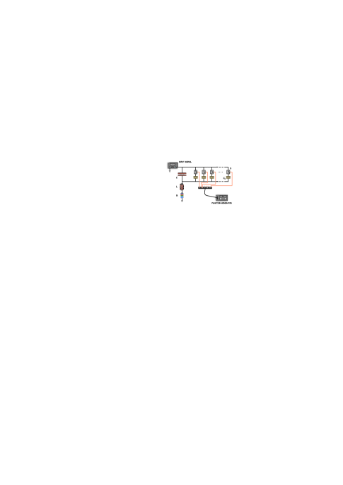
Figure 1: Scheme of the damped random-frequency electrical oscillator consisting of a RLC circuit with central capacitance $C$, inductance $L$ and a parasitic resistance $R$. Frequency fluctuations are achieved by switching on and off individual capacitors $C_{a}$ by means of analog switches $S$ that are driven by an arbitrary function generator.

Using the cumulant expansion described by Van Kampen van_kampen_book , Gitterman showed gitterman_book ; gitterman_2005 that the equation for $\left\langle x\right\rangle$, in the fast fluctuations regime, has the form (see Appendix for a detailed derivation)

$$\begin{split}\frac{d^{2}\left\langle x\right\rangle}{dt^{2}}+&\left(\Gamma+\frac{\omega_{0}^{4}}{2\nu^{2}}\text{c}_{2}\right)\frac{d\left\langle x\right\rangle}{dt}\\ &+\omega_{0}^{2}\left[1-\frac{\omega_{0}^{2}}{2\nu}\left(\text{c}_{1}-\frac{\Gamma}{2\nu}\text{c}_{2}\right)\right]\left\langle x\right\rangle=0,\end{split}$$ (2)

where $\nu=\left(\omega_{0}^{2}-\Gamma^{2}/4\right)^{1/2}$, and the coefficients $\text{c}_{1}$ and $\text{c}_{2}$ are defined by

$$\text{c}_{1} = \int_{0}^{\infty}\left\langle\phi\left(t\right)\phi\left(t-\xi\right)\right\rangle\sin\left(2\omega_{0}\xi\right)d\xi,$$ (3)

$$\text{c}_{2} = \int_{0}^{\infty}\left\langle\phi\left(t\right)\phi\left(t-\xi\right)\right\rangle\left[1-\cos\left(2\omega_{0}\xi\right)\right]d\xi.$$ (4)

Notice that, as pointed out in Ref. gitterman_book , the existence of frequency fluctuations in Eq. (1) introduces a noise-induced additional damping and a noise-induced frequency shift to the average signal of the oscillator.

III Experiment

III.1 The setup

The experimental setup that allows us to introduce random frequency fluctuations into a harmonic oscillator model is the following. Firstly, note that one can construct a system governed by Eq. (1) by making use of electrical $RLC$ oscillators (where $R$ stands for resistance, $L$ for inductance and $C$ for capacitance). In these systems, the charge in the capacitor satisfies the same equation as Eq. (1), where the coefficients $\Gamma$ and $\omega_{0}$ are defined by berthet_2003

$$\Gamma = R/L,$$ (5)

$$\omega_{0} = \left(LC_{0}\right)^{-1/2},$$ (6)

with $C_{0}$ denoting the average capacitance of the circuit. From Eq. (6) one can see that fluctuations in the frequency of the $RLC$ oscillator can be introduced by randomly switching the values of the capacitance explanation .

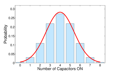
Figure 2: The probability that n-capacitors in the array are on follows a binomial distribution, which corresponds to a discretized Gaussian distribution with the same average and variance.

Random switching of capacitance is performed in the following way: An array of eight capacitors, each with equal capacitance $C_{a}$, is connected in parallel to a central capacitor $C$ of a $RLC$ circuit. To produce uncorrelated random switching, the individual capacitors are independently turned on/off by means of analog switches (NXP-74HC4066N quad bilateral switch), which are driven by independent digital signals provided by an arbitrary function generator (Signadyne digital I/O module SD-PXE-DIO-H0001), as shown in Fig. 1. Because we are interested in designing a Gaussian stochastic process, we program the arbitrary function generator, so each capacitor has the same probability to be on or off, in the same fashion as in a coin-tossing event. It is easy to show that the probability that $n$-capacitors in the array are on satisfies a binomial distribution given by

$$P\left(n\right)=\binom{8}{n}\frac{1}{2^{8}},$$ (7)

where $n=\{0,1,2,...,8\}$. This distribution is defined by a mean value $\left\langle n\right\rangle=4$ and a variance $\sigma^{2}_{b}=2$. Notice that the binomial distribution described in Eq. (7) is a discrete version of a Gaussian distribution with the same mean and variance, as depicted in Fig. 2. It is important to remark that due to the nonlinear relation between frequency and capacitance [Eq. (6)], when calculating the probability distribution of frequency, a Gaussian distribution is obtained provided that the condition $C_{a}\ll C$ is satisfied book_jacobs .

III.2 Implementation and Results

To test the proposed scheme, we construct a $RLC$ circuit where the central capacitance $C$ is provided by a 1 nF ceramic capacitor, inductance $L$ by a 1.5 mH ferrite core inductor, and resistance $R$ represents parasitic losses within the system. For the random switching of capacitance, we have designed several arrays using different ceramic capacitors with capacitance value $C_{a}=\{4.7,10,18,33,47,68,100\}$ pF. Notice from Fig. 2 that by changing the values of $C_{a}$ one can modify the variance of the Gaussian distribution, which in turn modifies the statistics of the noise in the system book_neuro .

To guarantee that our system is well described by Eq. (2), we make sure that frequency fluctuations are faster than the characteristic time evolution of the system, i.e., they satisfy the fast fluctuations condition gitterman_book . To this end, the digital signals from the arbitrary function generator are set with a time rate $\tau=650$ ns, which is longer than the response time of the analog switches ($400$ ns), and much shorter than the temporal evolution window of the measured signal ($t=100\;\mu$s).

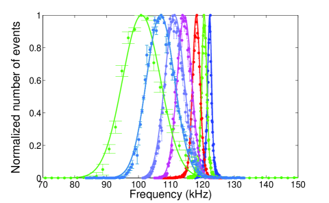
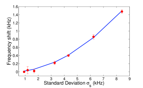
Figure 3: (a) Signal frequency histograms using different capacitor arrays. From left to right: $C_{a}=100,68,47,33,18,10,4.7$ pF. Dotted line: Experimental data, Solid line: Gaussian fitting. (b) Frequency shift as a function of the standard deviation $\sigma_{s}$. Dotted line: Experiment, Solid line: Theory.

Using the system described above, we have performed the simulation of Eq. (1). To this end, we keep the capacitor $C$ fixed and measure the averaged signal of the oscillator connected to different capacitor arrays. Figure 3(a) shows the histograms of the measured frequency in each case. Histograms are obtained from $50000$ different realizations, and they are normalized to the maximum number of events, where we define number of events as the number of realizations that have the same value of frequency. Notice that in all cases the probability distribution of the frequency follows a Gaussian distribution whose variance $\sigma_{s}^{2}$ depends strongly on the value of $C_{a}$ used in the connected array. This implies that this scheme allows to control the variance of the noise that is introduced in the system. Moreover, notice that by changing the way in which capacitors are turned on/off, one can modify the frequency probability distribution. For instance, a dichotomous-like random frequency could be obtained by switching on and off all capacitors at the same time.

To compare the results obtained in Fig. 3(a) with the theoretical model, we have measured the frequency shift that arises from the influence of frequency fluctuations, as predicted by Eq. (2). Figure 3(b) shows the frequency shift for each capacitor array. We have made use of Eq. (2), and the relation book_neuro : $D=\sigma^{2}\tau$, to find that the driving noise of our system can be described by a colored-noise-like autocorrelation function of the form

$$\left\langle\phi\left(t\right)\phi\left(t^{\prime}\right)\right\rangle=\frac{\sigma^{2}}{\omega_{0}^{2}}\exp\left(-\frac{\left|t-t^{\prime}\right|}{\tau}\right),$$ (8)

where the mean value of the frequency is computed with $C_{0}=C+4C_{a}$, and the variance of the driving noise is $\sigma^{2}=\left(\eta\sigma_{s}\right)^{2}$, with $\eta=3.4$. This relation between both variances can be understood as a consequence of the damping term in Eq. (1). The same effect can be found, for instance, in the Ornstein-Uhlenbeck process, where the resulting variance is proportional to the variance of the driving noise due to the presence of a damping term van_kampen_book .

In general, when simulating noise-induced transport effects, one is interested in keeping the mean frequency of each oscillator fixed while increasing the strength of the noise aspuru_2009 ; plenio_2008 ; roberto_2013 . This can be achieved in our system by controlling the values of the central capacitance $C$ and the time duration $\tau$ of the digital signals. Figure 4 shows the frequency histograms measured with different capacitor arrays. Notice that by properly controlling the parameters of the system, we are able to center all the probability distributions in the same value of frequency $f_{0}\simeq 123$ kHz. This demonstrates the flexibility of our system when modifying the statistical properties of the environmental noise that interacts with the oscillator. Parameters of the system used in each case are summarized in Table 1.

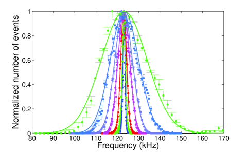
Figure 4: Frequency histograms for different capacitor arrays centered in the same mean frequency $f_{0}\simeq 123$ kHz. Dotted line: Experimental data, Solid line: Gaussian fitting.

$C_{a}$ (pF)		4.7	10	18	33	47	68	100
$C$ (nF)		1.120	1.090	1.053	0.978	0.933	0.840	0.355
$\tau$ (ns)		650	650	750	780	800	720	650

Table 1: Experimental parameters used to obtain the histograms shown in Fig. 4.

IV Conclusions and Outlook

In this paper, we have demonstrated a system that performs as a tunable environment for classical electrical oscillators. We have shown its operation by implementing the case of a damped random-frequency oscillator, where a perfect agreement with the theoretical model has been obtained. Finally, we have demonstrated the degree of control that one can achieve with this system by gradually modifying the variance of the frequency fluctuations, while maintaining a fixed central frequency of oscillation, which is of critical importance when simulating noise-induced energy transfer mechanisms in different scenarios, such as in the case of energy transfer in molecular aggregates.

The high degree of tunability and control of the proposed system can be further used to design various types of noise with different probability distributions. Moreover, it might allow us to study the transition from Markovian to non-Markovian dynamics of open systems. The results reported here represent an important step towards the experimental observation of Gaussian and non-Gaussian noise-induced transitions, and noise-induced transport effects.

Appendix A Derivation of the averaged amplitude equation of a damped random-frequency harmonic oscillator

Let us consider the equation for a damped random-frequency harmonic oscillator

$$\frac{d^{2}x}{dt^{2}}+\Gamma\frac{dx}{dt}+\omega^{2}_{0}\left[1+\alpha\phi\left(t\right)\right]x=0,$$ (9)

where $\Gamma$ is the damping coefficient, $\omega_{0}$ is the average frequency of the oscillator, and $\phi\left(t\right)$ is a dimensionless stochastic variable with zero average $\left\langle\phi\left(t\right)\right\rangle=0$, and an autocorrelation function satisfying $\langle\phi(t_{1})\phi(t_{2})\rangle\rightarrow 0$ for any two time points $t_{1}$, $t_{2}$ such that $|t_{2}-t_{1}|>\tau_{c}$, where $\tau_{c}$ is the correlation time of the stochastic process. To simplify the derivation of Eq. (2), and for consistency with Ref. van_kampen_book , we have included in Eq. (9) the parameter $\alpha$, which represents the strength of the stochastic fluctuations.

In order to solve Eq. (9), we first transform it into a set of first-order differential equations

$$\frac{d}{dt}X=\left(M_{\text{d}}+M_{\text{s}}\right)X,$$ (10)

where

$$X=\left[\begin{array}[]{c}x\left(t\right)\\ \dot{x}\left(t\right)\end{array}\right],$$ (11)

$$M_{\text{d}}=\left[\begin{array}[]{cc}0&1\\ -\omega_{0}^{2}&-\Gamma\end{array}\right],$$ (12)

$$M_{\text{s}}=\left[\begin{array}[]{cc}0&0\\ -\alpha\omega^{2}_{0}\phi\left(t\right)&0\end{array}\right].$$ (13)

Here, the matrices $M_{\text{d}}$ and $M_{\text{s}}$ represent the deterministic and stochastic evolution of the oscillator, respectively, and $\dot{x}\left(t\right)$ stands for the time derivative of the oscillator’s amplitude $x$.

In the matrix representation, it is easy to show that the equation for the deterministic evolution of the oscillator, i.e. $\dot{X}_{\text{d}}=M_{\text{d}}X_{\text{d}}$, has the solution

$$X_{\text{d}}\left(t\right)=U_{\text{d}}\left(t\right)X_{\text{d}}\left(0\right),$$ (14)

where

$$\begin{split}U_{\text{d}}\left(t\right)=\exp\left(-\frac{\Gamma}{2}t\right)\left[\begin{array}[]{cc}\cos\left(\nu t\right)+\left(\Gamma/2\nu\right)\sin\left(\nu t\right)&\sin\left(\nu t\right)/\nu\\ -\omega_{0}^{2}\sin\left(\nu t\right)/\nu&\cos\left(\nu t\right)-\left(\Gamma/2\nu\right)\sin\left(\nu t\right)\end{array}\right].\end{split}$$ (15)

Notice that the presence of damping in the harmonic oscillator produces a frequency shift that is given by $\nu=\sqrt{\omega_{0}^{2}-\Gamma^{2}/4}$.

Now, we make use of Eq. (15) to perform the transformation

$$X\left(t\right)=U_{\text{d}}\left(t\right)\tilde{X}\left(t\right),$$ (16)

which by substituting it into Eq. (10) allows us to write

$$\frac{d}{dt}\tilde{X}=\alpha U_{\text{d}}\left(-t\right)M_{\text{s}}\left(t\right)U_{\text{d}}\left(t\right)\tilde{X}\left(t\right).$$ (17)

Then, we iteratively solve Eq. (17) to find that the average of $\tilde{X}$ writes

$$\begin{split}\langle\tilde{X}\left(t\right)\rangle=&\langle\tilde{X}\left(0\right)\rangle+\alpha^{2}\int_{0}^{t}dt_{1}\int_{0}^{\infty}dt_{2}\langle U_{\text{d}}\left(-t_{1}\right)M_{\text{s}}\left(t_{1}\right)\\ &\times U_{\text{d}}\left(t_{1}-t_{2}\right)M_{\text{s}}\left(t_{2}\right)U_{\text{d}}\left(t_{2}\right)\rangle\langle\tilde{X}\left(0\right)\rangle.\end{split}$$ (18)

Notice that the linear term with $\alpha$ disappears since $\langle M_{\text{s}}\left(t\right)\rangle=0$. In writing Eq. (18), we have considered only the contributions up to $\alpha^{2}$, which is an approximation that is valid as long as the condition $\alpha\tau_{c}\ll 1$ is satisfied. In addition, we have assumed that the correlation time $\tau_{c}$ is much shorter than the integration time, so we can take $\langle\tilde{X}\left(t\right)\rangle\rightarrow\langle\tilde{X}\left(0\right)\rangle$, and integrate to infinity, in the second term of Eq. (18).

We now perform the time derivative of Eq. (18) to obtain

$$\begin{split}\frac{d}{dt}\langle\tilde{X}\left(t\right)\rangle=&\alpha^{2}\int_{0}^{\infty}d\xi\langle U_{\text{d}}\left(-t\right)M_{\text{s}}\left(t\right)U_{d}\left(\xi\right)M_{\text{s}}\left(t-\xi\right)\\ &\times U_{\text{d}}\left(t-\xi\right)\rangle\langle\tilde{X}\left(0\right)\rangle,\end{split}$$ (19)

where the substitutions $\xi=t_{1}-t_{2}$, and $t=t_{1}$ are used. Inverse transformation of Eq. (19), by means of Eq. (16), then gives

$$\begin{split}\frac{d}{dt}\langle X\left(t\right)\rangle=&\left[M_{\text{d}}+\alpha^{2}\int_{0}^{\infty}d\xi\langle M_{\text{s}}\left(t\right)U_{\text{d}}\left(\xi\right)\right.\\ &\times M_{\text{s}}\left(t-\xi\right)U_{\text{d}}\left(-\xi\right)\rangle\bigg{]}\langle X\left(t\right)\rangle.\end{split}$$ (20)

Using Eqs. (13) and (15), we can readily find that the expression inside the integral of Eq. (20) writes

$$\begin{split}\langle M_{\text{s}}\left(t\right)U_{\text{d}}\left(\xi\right)M_{\text{s}}\left(t-\xi\right)U_{\text{d}}\left(-\xi\right)\rangle=&\omega_{0}^{4}\langle\phi\left(t\right)\phi\left(t-\xi\right)\rangle\\ &\times\left\{\begin{array}[]{cc}0&0\\ \left[\sin\left(\nu\xi\right)/\nu\right]\left[\cos\left(\nu\xi\right)-\left(\Gamma/2\nu\right)\sin\left(\nu\xi\right)\right]&-\sin^{2}\left(\nu\xi\right)/\nu^{2}\end{array}\right\}.\end{split}$$ (21)

Finally, by substituting Eq. (21) into Eq. (20), and transforming the set of two first-order equations to a single second-order differential equation, Eq. (2) is obtained.

References

- (1) L. Gammaitoni, P. Hänggi, P. Jung, and F. Marchesoni, Rev. Mod. Phys. 70, 223 (1998).
- (2) W. Horsthemke and R. Lefever, Noise-Induced Transitions: Theory and Applications in Physics, Chemistry, and Biology (Springer, Berlin, 1984).
- (3) C. Van den Broeck, J. M. R. Parrondo, and R. Toral, Phys. Rev. Lett. 73, 3395 (1994).
- (4) P. Rebentrost, M. Mohseni, I. Kassal, S. Lloyd, and A. Aspuru-Guzik, New J. Phys. 11, 033003 (2009).
- (5) M. Plenio and S. Huelga, New J. Phys. 10, 113019 (2008).
- (6) P. Hänggi and F. Marchesoni, Rev. Mod. Phys. 81, 387 (2009).
- (7) R. de J. León-Montiel and Juan P. Torres, Phys. Rev. Lett. 110, 218101 (2013).
- (8) T. Kawakubo, S. Kabashima, and Y. Tsuchiya, Progr. Theor. Phys. 64, 150 (1978).
- (9) S. Kabashima and T. Kawakubo, Phys. Lett. A 70, 375 (1979).
- (10) S. Kabashima, S. Kogure, T. Kawakubo, and T. Okada, J. Appl. Phys. 50, 6296 (1979).
- (11) R. Berthet, A. Petrossian, S. Residori, B. Roman, and S. Fauve, Physica D 174, 84 (2003).
- (12) S. Residori, R. Berthet, B. Roman, and S. Fauve, Phys. Rev. Lett. 88, 024502 (2001).
- (13) V. V. Zautkin, B. I. Orel, and V. B. Cherepanov, Sov. Phys. JETP 58, 414 (1983).
- (14) T. John, R. Stannarius, and U. Behn, Phys. Rev. Lett. 83, 749 (1999).
- (15) H. S. Wio and R. Toral, Physica D 193, 161 (2004).
- (16) M. A. Fuentes, R. Toral, and H. S. Wio, Physica A 295, 114 (2001).
- (17) F. J. Castro, M. N. Kuperman, M. Fuentes, and H. S. Wio, Phys. Rev. E 64, 051105 (2001).
- (18) S. Bouzat and H. S. Wio, Eur. Phys. J. B 41, 97 (2004).
- (19) M. Gitterman, The Noisy Oscillator: The First Hundred Years, From Einstein Until Now (World Scientific, Singapore, 2005).
- (20) R. Graham, M. Höhnerbach, and A. Schenzle, Phys. Rev. Lett. 48, 1396 (1982).
- (21) A. Ishimaru, Wave Propagation and Scattering in Random Media (IEEE Press, Piscataway, NJ, 1997).
- (22) M. Turelli, Theoretical Population Biology 12, 140 (1977).
- (23) H. Takayasu, A.-H. Sato, and M. Takayasu, Phys. Rev. Lett. 79, 966 (1997).
- (24) M. Gitterman and D. A. Kessler, Phys. Rev. E 87, 022137 (2013).
- (25) M. Gitterman, Physica A 352, 309 (2005).
- (26) C. Laing and G. J. Lord, Stochastic Methods in Neuroscience (Clarendon Press, Oxford, 2008)
- (27) N. G. Van Kampen, Stochastic Processes in Physics and Chemistry (Elsevier, The Netherlands, 2007).
- (28) For the sake of simplicity, we have selected a random switching of the capacitance. However, one can always choose to randomly change the values of the inductance. By doing this, one adds more complexity to the system since the damping coefficient would randomly fluctuate as well.
- (29) K. Jacobs, Stochastic Processes for Physicists: Understanding Noisy Systems (Cambridge University Press, UK, 2010).