$B$ decays to two pseudoscalars and a generalized $\Delta I=\frac{1}{2}$ rule

Abstract

We perform an isospin analysis of $B$ decays to two pseudoscalars. The analysis extracts appropriate CKM and short distance loop factors to allow for comparison of non-perturbative QCD effects in the reduced matrix elements of the amplitudes. In decays where penguin diagrams compete with tree-level diagrams we find that the reduced matrix elements of the penguin diagrams, which are singlets or doublets under isospin, are significantly enhanced compared with the triplet and fourplet contributions of the weak Hamiltonian. This similarity to the $\Delta I=\frac{1}{2}$ rule in $K\to\pi\pi$ decays suggests that, more generally, processes mediated by Hamiltonians in lower-dimensional isospin representations see enhancement over higher-dimensional ones in QCD.

I Introduction

One of the longstanding puzzles in flavor physics is the $\Delta I=1/2$ rule. An isospin-$\tfrac{1}{2}$ neutral kaon may decay into two pions in either an isospin-0 or isospin-2 ($s$-wave) state with amplitude $A_{0}$ or $A_{2}$, respectively. Empirically,

$$\frac{\text{Re}\,A_{0}}{\text{Re}\,A_{2}}=22.5~{}.$$ (1)

The $\Delta I=1/2$ rule is the statement that the amplitude $A_{0}$, mediated by the part of the weak Hamiltonian that transforms as an $I=1/2$ tensor, is much larger than $A_{2}$, mediated by the larger $I=3/2$ tensor.

There is no satisfactory understanding of this rule. In Refs. Bardeen et al. (1986, 1987a, 1987b) and, more recently, Ref. Buras et al. (2014) the rule was investigated in chiral perturbation theory, in the large $N_{c}$ limit. However, it was argued in Ref. Chivukula et al. (1986) that for QCD, $N_{c}=3$ is not large enough for this limit to be useful. More recent studies using Monte Carlo simulations of QCD in the lattice have addressed the $\Delta I=1/2$ rule Blum et al. (2012); a very recent study on the lattice of the validity of the vacuum insertion approximation was done in Carrasco et al. (2013). The ratio in (1) is still twice as large as any values obtained on the lattice with unphysical quark masses, but it is expected that simulations at physical quark masses will reproduce the empirically observed ratio and shed light on the origin of the enhancement Boyle et al. (2013). This begs the question– does this enhancement occur in systems other than the $K\to\pi\pi$ system?

There is evidence that answers this question in the affirmative. Identifying any patterns of enhancements will give new insights into the long distance dynamics of QCD. For example, the $SU(3)$ analysis of $D\to KK,\pi\pi$ decays reveals a similar enhancement. In that system, the $D^{0}\to K^{+}K^{-}$ and $D^{0}\to\pi^{+}\pi^{-}$ amplitudes may be written as Quigg (1980)

$$\mathcal{A}(D^{0}\to K^{+}K^{-}) =(2T+E-S)\Sigma$$

$$+\tfrac{1}{2}(3T+2G+F-E)\Delta$$

$$\mathcal{A}(D^{0}\to\pi^{+}\pi^{-}) =-(2T+E-S)\Sigma$$

$$+\tfrac{1}{2}(3T+2G+F-E)\Delta$$

where $\Sigma\equiv\tfrac{1}{2}(V^{*}_{cs}V^{\phantom{*}}_{us}-V^{*}_{cd}V^{\phantom{*}}_{ud})$ and $\Delta\equiv\tfrac{1}{2}(V^{*}_{cs}V^{\phantom{*}}_{us}+V^{*}_{cd}V^{\phantom{*}}_{ud})$. $S$, $E$ and $F$ are the invariant matrix elements between a $D$ meson and a meson pair in an octet of the $\mathbf{\bar{6}}$, 15 and 3 components of the weak Hamiltonian, respectively, $G$ of the 3 to a singlet pair and $T$ of the 15 to a meson pair in the 27. Note that $\Sigma\approx\lambda=\sin\theta_{C}$, while $|\Delta|\sim\lambda^{5}$, so that $|\Delta|/\Sigma\sim 10^{-3}$. Neglecting $\Delta$ one would have $\Gamma(D^{0}\to K^{+}K^{-})=\Gamma(D^{0}\to\pi^{+}\pi^{-})$ in the $SU(3)$ limit. Experimentally $\Gamma(D^{0}\to K^{+}K^{-})/\Gamma(D^{0}\to\pi^{+}\pi^{-})\approx 3$ requires both the $\Sigma$ and $\Delta$ terms in the amplitude to contribute with similar strengths. Barring accidental cancellations this means that the matrix elements $G$ and $F$ are significantly enhanced. Since $\Delta$ has a large phase, significant CP-violation in these decays was predicted Golden and Grinstein (1989) and recently confirmed by experiment Aaltonen et al. (2012a, b); Aaij et al. (2013).

If $SU(3)$-breaking effects are included, the ratio $\Gamma(D^{0}\to K^{+}K^{-})/\Gamma(D^{0}\to\pi^{+}\pi^{-})\approx 3$ can be attained with only a “mild” enhancement of $F$ and $G$ relative to the other reduced matrix elements of about an order of magnitude Pirtskhalava and Uttayarat (2012); Bhattacharya et al. (2012); Feldmann et al. (2012); Brod et al. (2012); Cheng and Chiang (2012); Hiller et al. (2013). The enhancement in $F$ and $G$ is similar to that of the $\Delta I=1/2$ rule in that it appears in matrix elements of the smallest $SU(3)$-representation of the Hamiltonian. In this case, the dominant contributions are from the 3 Hamiltonian (as opposed to the $\mathbf{\bar{6}}$ and 15), whereas for the $\Delta I=1/2$ rule the dominant piece is from the $I=1/2$ Hamiltonian (as opposed to the $I=3/2$ piece).

In this work we investigate the possibility of similar enhancements in $B$ decays. We will show that an isospin analysis of $B\to K\pi$ decays and CP-asymmetries shows a marked enhancement of amplitudes mediated by the weak Hamiltonian in the lowest isospin representation. An analysis of $B\to\pi\pi$ decays shows that, although there is little enhancement of doublet versus fourplet amplitudes, the matrix elements of penguin contributions (which are purely $\Delta I=1/2$) are still enhanced to produce the observed data. Both these analyses support the general rule that amplitudes mediated by the piece of the weak Hamiltonian in the smallest representation of the symmetry group are enhanced.

It should go without saying that we have no dynamical explanation of the enhancement. This comes as no surprise, since the very $\Delta I=1/2$ rule has resisted explanation for more than a half century. But we hope that insights provided by this new, generalized rule may eventually lead to a global understanding of these enhancements.

II Isospin analysis

The strong interactions, to a good approximation, obey isospin symmetry. In hadronic spectra and decays isospin violating effects are no larger than a few per cent. We study the amplitudes for the decay of $B$-mesons to two light scalar mesons using isospin symmetry, under which kaons and $B$-mesons transform as doublets and pions as a triplet. The possible two-body final states are easily classified according to their transformation properties under isospin. We also need the transformation properties of the effective Hamiltonian responsible for the weak decay. The effective Hamiltonian is given in terms of four-quark operators, whose transformation properties are readily determined.

II.1 $B\to K\pi$

The effective Hamiltonian density for the $\Delta B=-1$, $\Delta S=-1$ decays, to leading order in the Fermi constant $G_{F}$, can be written as Buras (1998); Buchalla et al. (1996)

$$\mathcal{H}=\frac{G_{F}}{\sqrt{2}} \left[\lambda_{u}\left(C_{1}Q_{1}+C_{2}Q_{2}\right)-\lambda_{t}\sum_{i=3}^{6}C_{i}Q_{i}\right].$$ (2)

Here $\lambda_{q}\equiv V^{*}_{qb}V_{qs}$ are CKM factors and $C_{i}$’s are the Wilson coefficients. The “tree” ($Q_{1,2}$) and “penguin” ($Q_{3-6}$) operators are defined as

$$Q_{1} =\left(\bar{b}_{a}u_{b}\right)_{V-A}\left(\bar{u}_{b}s_{a}\right)_{V-A},$$

$$Q_{2} =\left(\bar{b}u\right)_{V-A}\left(\bar{u}s\right)_{V-A},$$

$$Q_{3} =\left(\bar{b}s\right)_{V-A}\sum_{q=u,d}\left(\bar{q}q\right)_{V-A},$$

$$Q_{4} =\left(\bar{b}_{a}s_{b}\right)_{V-A}\sum_{q=u,d}\left(\bar{q}_{b}q_{a}\right)_{V-A},$$

$$Q_{5} =\left(\bar{b}s\right)_{V-A}\sum_{q=u,d}\left(\bar{q}q\right)_{V+A},$$

$$Q_{6} =\left(\bar{b}_{a}s_{b}\right)_{V-A}\sum_{q=u,d}\left(\bar{q}_{b}q_{a}\right)_{V+A}$$ (3)

where $(\bar{q}q)_{V\pm A}$ is shorthand for $\bar{q}\gamma^{\mu}(1\pm\gamma^{5})q$. Both the coefficients $C_{i}$ and the matrix elements of the operators $Q_{i}$ depend on an arbitrary renormalization point $\mu$ but their combination in the Hamiltonian, Eq. (2), is $\mu$-independent. QCD-penguins arising from $u$ and $c$ quark loops combine into terms precisely of the form of top-quark penguins, since $\lambda_{c}+\lambda_{u}=-\lambda_{t}$. We have also neglected electroweak penguins (EWP), operators $Q_{7-10}$ in Ref.  Buras (1998). These introduce new isospin triplets into the Hamiltonian with a $\lambda_{t}$ coefficient, suppressed relative to the top-penguins by $\alpha/\alpha_{s}$. We have ignored EWP contributions out of pragmatism: were we to include their effects in our fits the number of unknown matrix elements would exceed the number of measured data. But our pragmatism is informed: the coefficients of EWP in the effective Hamiltonian are suppressed relative to QCD penguins roughly by a factor of $\alpha/\alpha_{s}$, or about 7% if evaluated at $\mu=M_{Z}$ and smaller at $m_{b}$. As will become evident, the approximation is supported by the very good fit of the model to both $B\to K\pi$ and $B\to\pi\pi$ processes.

Mode	$\mathcal{B}$ ($10^{-6}$)	$A_{CP}$	$C_{f}$	$S_{f}$
$B^{+}\to K^{+}\pi^{0}$	$12.9\pm 0.5$	$\phantom{-}0.037\pm 0.021$	–	–
$B^{+}\to K^{0}\pi^{+}$	$23.8\pm 0.7$	$-0.014\pm 0.019$	–	–
$B^{0}_{d}\to K^{0}\pi^{0}$	$\phantom{1}9.9\pm 0.5$	–	$0.00\pm 0.13$	$0.58\pm 0.17$
$B^{0}_{d}\to K^{+}\pi^{-}$	$19.6\pm 0.5$	$-0.087\pm 0.008$	–	–

Table 1: Data available in $B\to K\pi$ decays Beringer et al. (2012). The $C$ and $S$ parameters are measured for decays into the final CP eigenstate, $B^{0}_{d}\to K^{0}_{s}\pi_{0}$. The amplitude for $B^{0}_{d}\to K^{0}\pi^{0}$ on the other hand is given as $\mathcal{A}(B^{0}_{d}\to K^{0}\pi^{0})=\sqrt{2}~{}\mathcal{A}(B^{0}_{d}\to K^{0}_{s}\pi^{0}).$

As far as the group theory analysis of rates and CP asymmetries is concerned, different four-quark operators contributing to the Hamiltonian can be distinguished solely by their isospin quantum numbers and CKM factors. The Hamiltonian can therefore be compactly written in terms of the isospin representations in the following way:

$$H=V^{*}_{ub}V_{us}~{}\left(\mathbf{1}+[\mathbf{3}]^{1}_{~{}1}\right)+\frac{\alpha_{s}}{8\pi}~{}V^{*}_{tb}V_{ts}~{}\mathbf{1^{\prime}}~{},$$ (4)

where $\mathbf{1}$ ($\mathbf{1^{\prime}}$) denotes the singlet coming from the tree (penguin) operators, $[\mathbf{3}]^{1}_{~{}1}$ represents the triplet operator, and $\alpha_{s}$ the strong coupling constant evaluated at $M_{Z}$. We choose to normalize the singlet penguin operator with an agnostic factor of $\alpha_{s}/(8\pi)$ to make explicit the loop factor associated with it. This normalization does not affect the results of this paper, but it is a useful choice that, naïvely, would give reduced matrix element values of the same order of magnitude for every contribution. We introduce shorthand for the reduced matrix elements, as follows:

$$\langle\mathbf{\bar{2}|1|}B\rangle\equiv P_{b},\quad\langle\mathbf{\bar{2}|\mathbf{1^{\prime}}|}B\rangle\equiv P_{a},$$

$$\langle\mathbf{\bar{2}|3|}B\rangle\equiv T,\quad\langle\mathbf{\bar{4}|3|}B\rangle\equiv S~{}.$$ (5)

While we cannot compute $P_{a}$, $P_{b}$, $S$ and $T$ from first principles, we can determine them by fitting to experimental measurements of decay rates and CP asymmetries.

In terms of the reduced matrix elements in Eq. (II.1), the isospin decomposition of the decay amplitudes is

$$\mathcal{A}(B^{+}\to K^{+}\pi^{0}) =V^{\ast}_{ub}V^{\phantom{\ast}}_{us}~{}\frac{1}{\sqrt{2}}\left(P_{b}+T+2S\right)$$

$$+\,\frac{\alpha_{s}}{8\pi}~{}V^{\ast}_{tb}V^{\phantom{\ast}}_{ts}~{}\frac{P_{a}}{\sqrt{2}}~{},$$

$$\mathcal{A}(B^{+}\to K^{0}\pi^{+}) =V^{\ast}_{ub}V^{\phantom{\ast}}_{us}~{}\left(P_{b}+T-S\right)$$

$$+\,\frac{\alpha_{s}}{8\pi}~{}V^{\ast}_{tb}V^{\phantom{\ast}}_{ts}~{}P_{a}~{},$$

$$\mathcal{A}(B^{0}\to K^{0}\pi^{0}) =V^{\ast}_{ub}V^{\phantom{\ast}}_{us}~{}\frac{1}{\sqrt{2}}~{}\left(-P_{b}+T+2S\right)$$

$$-\,\frac{\alpha_{s}}{8\pi}~{}V^{\ast}_{tb}V^{\phantom{\ast}}_{ts}~{}\frac{P_{a}}{\sqrt{2}},$$

$$\mathcal{A}(B^{0}\to K^{+}\pi^{-}) =V^{\ast}_{ub}V^{\phantom{\ast}}_{us}~{}\left(P_{b}-T+S\right)$$

$$+\,\frac{\alpha_{s}}{8\pi}~{}V^{\ast}_{tb}V^{\phantom{\ast}}_{ts}~{}P_{a}~{}.$$ (6)

There is a contribution proportional to $V^{\ast}_{ub}V^{\phantom{\ast}}_{us}$ to the amplitude $\mathcal{A}\left(B^{+}\to K^{0}\pi^{+}\right)$. The only contribution to this process stems from the annihilation diagram, shown in Fig. 1. There is extensive literature on annihilation diagram suppression with respect to $W$-emission diagrams Chau et al. (1991); Gronau et al. (1994). To evaluate this expectation, denote the matrix element associated with the annihilation diagram by $M\equiv P_{b}+T-S$ and let $|M|=x|P_{a}|$ so that $x$ measures the relative importance of annihilation in comparison to the top-loop penguin. The value of $x$ for which the annihilation and penguin contributions to $B^{+}\to K^{0}\pi^{+}$ are of the same order can be estimated as

$$x=\frac{\alpha_{s}}{8\pi}~{}\bigg{|}\frac{V^{\ast}_{tb}V^{\phantom{\ast}}_{ts}}{V^{\ast}_{ub}V^{\phantom{\ast}}_{us}}\bigg{|}\simeq 0.24~{}.$$ (7)

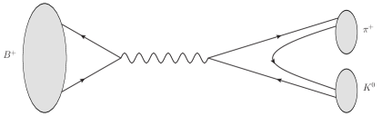
Figure 1: Leading order diagram contributing to the $B^{+}\to K^{0}\pi^{+}$ process.

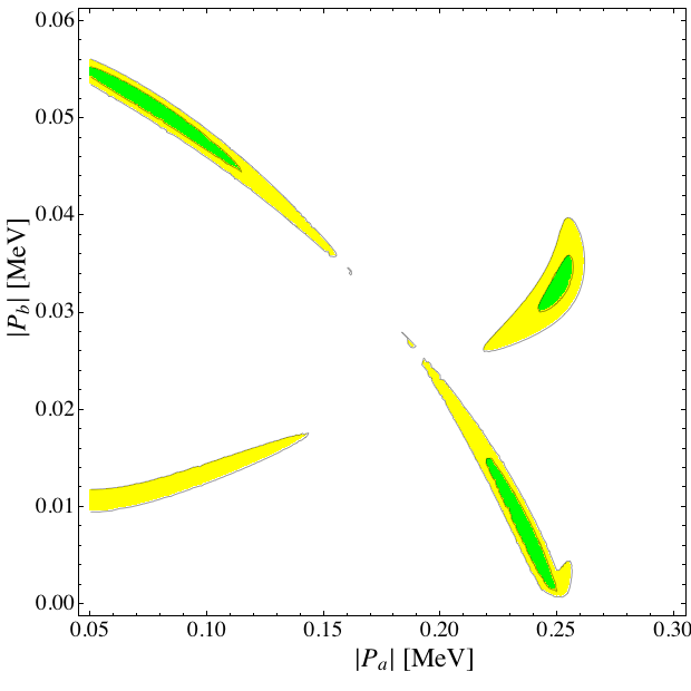
(a)

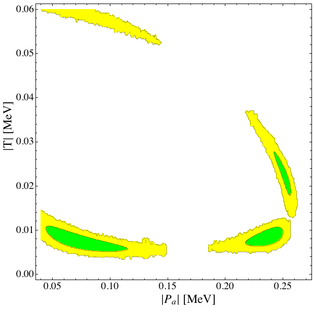
(b)

Figure 2: Fit to data of the reduced matrix elements for $B\to K\pi$. The figures show the 68% (green) and 95% (yellow) CL regions in the $|P_{a}|$ vs $|P_{b}|$ and $|P_{a}|$ vs $|T|$ planes. The raggedness of the contours is an artifact of the numerical computation.

Results of the fit

The available decay data for $B\to K\pi$ are collected in Table 1; the observables are defined in Appendix A. Performing a $\chi^{2}$ fit of matrix elements in Eq. (II.1) to the data, we find values for the matrix elements that match the observed data with a 95% confidence level. These minima are illustrated with 68% and 95% confidence levels in the $|P_{a}|$ vs. $|P_{b}|$ and $|P_{a}|$ vs. $|T|$ planes, respectively, in Fig. 2. The best fit has $\{|P_{a}|,\,|P_{b}|,\,|T|,\,|S|\}\simeq\{0.237,\,7.2\times 10^{-3},\,8.4\times 10^{-3},\,2.2\times 10^{-3}\}$ MeV with a chi-squared of ${\chi}^{2}=1.70$ for two degrees of freedom (a common phase in the reduced matrix elements is unobservable). The $\Delta I=0$ contribution to the amplitudes, from the Hamiltonian in the singlet representation, is given by the quantity

$$a_{\Delta I=0}=P_{b}+\frac{\alpha_{s}}{8\pi}~{}\frac{V^{\ast}_{tb}V^{\phantom{\ast}}_{ts}}{V^{\ast}_{ub}V^{\phantom{\ast}}_{us}}P_{a}$$ (8)

and the $\Delta I=1$ contribution, from the triplet Hamiltonian, by

$$a_{\Delta I=1}=\{T+2S,T-S\}.$$ (9)

for $\left(B^{+}\to K^{+}\pi^{0},B^{0}\to K^{0}\pi^{+}\right)$ and $\left(B^{+}\to K^{0}\pi^{+},B^{0}\to K^{+}\pi^{-}\right)$ respectively. For the best fit then, we find

$$\bigg{|}\frac{a_{\Delta I=0}}{a_{\Delta I=1}}\bigg{|}=\{4.8,~{}9.9\}$$ (10)

which is reminiscent of the $\Delta I=\tfrac{1}{2}$ rule from $K\to\pi\pi$ decays.

A second, slightly higher $\chi^{2}$-minimum has $\{|P_{a}|,\,|P_{b}|,\,|T|,\,|S|\}\simeq\{0.075,\,0.052,\,7.3\times 10^{-3},\,2.4\times 10^{-3}\}$ MeV with a chi-squared of ${\chi}^{2}=1.80$ and

$$\bigg{|}\frac{a_{\Delta I=0}}{a_{\Delta I=1}}\bigg{|}=\{5.2,~{}12.6\}~{}.$$ (11)

Both of these minima have significant enhancement of the penguin singlet, $P_{a}$, over the triplet matrix elements, $T$ and $S$. In the best fit case, however, the other singlet matrix element, $P_{b}$, does not show significant enhancement over the triplet matrix elements. Consequently, the annihilation diagram contribution is negligible in the best fit ($|M|=0.013$ MeV or, equivalently, $x=|M/P_{a}|=0.055$, to be compared with Eq. (7)) but provides a larger contribution than that of the penguin diagram in the second best fit (where $|M|=0.055$ MeV or, equivalently, $x=0.732$).

For completeness we note that there are two additional minima corresponding to $\chi^{2}=3.04$ and 4.34. These two minima are less favorable, so we ignore them in the rest of our study.

In all but the least favored minimum, there is significant enhancement of $|P_{a}|$ over the triplet Hamiltonian matrix elements. Moreover, the total contribution from the $\Delta I=0$ Hamiltonian, $a_{\Delta I=0}$, enjoys an enhancement over the $\Delta I=1$ contribution, $a_{\Delta I=1}$. More precise data will be welcomed to distinguish between these minima, which would also decide the role of the annihilation diagram in these decays.

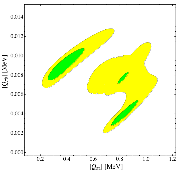
(a)

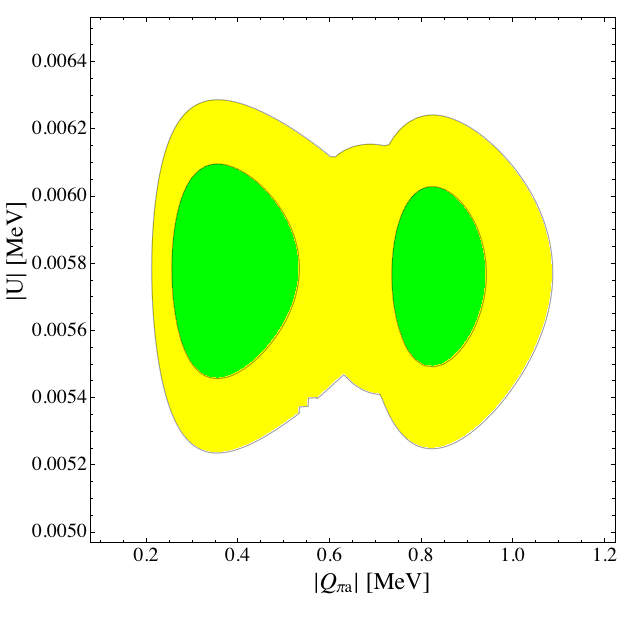
(b)

Figure 3: Fit to data of the reduced matrix elements for $B\to\pi\pi$. The figures show the 68% (green) and 95% (yellow) CL regions in the $|Q_{\pi a}|$ vs $|Q_{\pi b}|$ and $|Q_{\pi a}|$ vs $|U|$ planes. The raggedness of the contours is an artifact of the numerical computation.

II.2 $B\to\pi\pi$

The isospin analysis for $\pi\pi$ final states is analogous to that for $K$ decays, where the $\Delta I=\tfrac{1}{2}$ rule was discovered. Operator contributions are of the form in (II.1), but for $\Delta S=0$ processes. The Hamiltonian decomposes under isospin as $\mathbf{\bar{2}\times 2\times\bar{2}=\bar{2}+\bar{2}+\bar{4}}$ so that

$$H=V^{*}_{ub}V_{ud}~{}\left([\mathbf{\bar{2}}]^{2}+[\mathbf{\bar{4}}]^{12}_{1}\right)+\frac{\alpha_{s}}{8\pi}~{}V^{*}_{tb}V_{ts}~{}[\mathbf{\bar{2}^{\prime}}]^{2}~{},$$ (12)

The final states transform as $(\mathbf{3}\times\mathbf{3})_{S}=\mathbf{1}+\mathbf{5}$, so the non-vanishing reduced matrix elements are

$$\langle\mathbf{1|2^{\prime}|}B\rangle=Q_{\pi a},\;\langle\mathbf{1|2|}B\rangle=Q_{\pi b},\;\langle\mathbf{5|4|}B\rangle=U$$ (13)

and the decay amplitudes relevant to the processes in Table 2 are

$$\mathcal{A}(B^{+}\to\pi^{+}\pi^{0}) =\sqrt{\frac{3}{2}}~{}V^{\ast}_{ub}V^{\phantom{\ast}}_{ud}~{}\,U~{},$$

$$\mathcal{A}(B^{0}\to\pi^{0}\pi^{0}) =V^{\ast}_{ub}V^{\phantom{\ast}}_{ud}~{}\frac{1}{\sqrt{3}}\left(Q_{\pi b}-\sqrt{2}\,U\right)$$

$$+\frac{\alpha_{s}}{8\pi}~{}V^{\ast}_{tb}V^{\phantom{\ast}}_{td}~{}\frac{1}{\sqrt{3}}Q_{\pi a}~{},$$

$$\mathcal{A}(B^{0}\to\pi^{+}\pi^{-}) =V^{\ast}_{ub}V^{\phantom{\ast}}_{ud}~{}\frac{1}{\sqrt{3}}\left(\sqrt{2}\,Q_{\pi b}+U\right)$$

$$+\frac{\alpha_{s}}{8\pi}~{}V^{\ast}_{tb}V^{\phantom{\ast}}_{td}~{}\sqrt{\frac{2}{3}}\,Q_{\pi a}~{}.$$ (14)

Results of the fit

Mode	$\mathcal{B}$ ($10^{-6}$)	$A_{CP}$	$C_{f}$	$S_{f}$
$B^{+}\to\pi^{+}\pi^{0}$	$5.5\pm 0.4$	$0.03\pm 0.04$	–	–
$B^{0}\to\pi^{0}\pi^{0}$	$1.91^{\pm}0.22$	–	$-0.43\pm 0.24$	–
$B^{0}\to\pi^{+}\pi^{-}$	$5.12\pm 0.19$	–	$-0.38\pm 0.15$	$-0.65\pm 0.07$

Table 2: Data available in $B\to\pi\pi$ decays from Ref Beringer et al. (2012).

The data available in this decay channel are listed in Table  2. We perform a $\chi^{2}$-fit of the model, Eq. (II.2), to the data. The result of the fit is illustrated with 68% (green) and 95% (yellow) CL regions in the $|Q_{\pi a}|$ vs $|Q_{\pi b}|$ and $|Q_{\pi a}|$ vs $|U|$ planes, respectively, in Fig. 3. For the best fit to the data we obtain $\{|Q_{\pi a}|,~{}|Q_{\pi b}|,~{}|U|\}\simeq\{0.35,~{}8.8\times 10^{-3},~{}5.8\times 10^{-3}\}$ MeV with a chi-squared of ${\chi}^{2}\simeq 1.39$ for 2 degrees of freedom. Two additional regions with a good fit to the data are found, one with $\{|Q_{\pi a}|,~{}|Q_{\pi b}|,~{}|U|\}\simeq\{0.82,~{}3.9\times 10^{-3},~{}5.8\times 10^{-3}\}$ MeV for a chi-squared of ${\chi}^{2}\simeq 2.07$ and the other with $\{|Q_{\pi a}|,~{}|Q_{\pi b}|,~{}|U|\}\simeq\{0.82,~{}7.7\times 10^{-3},~{}5.8\times 10^{-3}\}$ MeV for a chi-squared of ${\chi}^{2}\simeq 3.38$. Since the last minimum is less favorable, we will ignore it. The contribution to the amplitudes from the Hamiltonian in the doublet representation is

$$a_{\Delta I=1/2}=Q_{\pi b}+\frac{\alpha_{s}}{8\pi}\frac{V^{*}_{tb}V_{td}}{V^{*}_{ub}V_{ud}}Q_{\pi a}$$ (15)

and from the fourplet Hamiltonian

$$a_{\Delta I=3/2}=U.$$ (16)

We find no enhancement of the $\Delta I=1/2$ amplitude with respect to the $\Delta I=3/2$ amplitude. To wit, for the best fits (next favorable minimum) we find

$$\bigg{|}\frac{a_{\Delta I=1/2}}{a_{\Delta I=3/2}}\bigg{|}=1.04\,(1.05).$$ (17)

There is little enhancement of the reduced matrix element corresponding to the tree-level doublet Hamiltonian, $Q_{\pi b}$, with respect to the tree-level quadruplet $U$. However, the large enhancement of the penguin doublet reduced matrix element $Q_{\pi a}$ over $U$ is analogous to that in the $K\to\pi\pi$ decays, which has identical isospin analysis to the $B\to\pi\pi$ case. That a similar enhancement exists in the $B$ system —both in $K\pi$ and $\pi\pi$ final states— is striking, and cries out for a dynamical explanation of the role of flavor symmetries in these enhancements.

II.3 $B\to K\overline{K}$

Mode	$\mathcal{B}$ ($10^{-6}$)	$A_{CP}$	$C_{f}$	$S_{f}$
$B^{+}\to K^{+}\overline{K}^{0}$	$1.19\pm 0.18$	$0.04\pm 0.14$	–	–
$B^{0}\to K^{+}K^{-}$	$0.13\pm 0.05$	–	–	–
$B^{0}\to K^{0}\overline{K}^{0}$	$1.21\pm 0.16$	$-0.6\pm 0.7$	$0.0\pm 0.4$	$-0.8\pm 0.5$

Table 3: Data available in $B\to K\bar{K}$ decays Beringer et al. (2012).

At leading order, decays of B mesons to kaons proceed via the $\Delta S=0$ Hamiltonian in (12). The $K$ ($\bar{K}$) transforms as a $\mathbf{2}$ ($\mathbf{\bar{2}}$) under isospin, so the final states decompose under isospin as $\mathbf{2\times\bar{2}=1+3}$.

The reduced matrix elements are then $\langle\mathbf{1|2^{(\prime)}}|B\rangle$, $\langle\mathbf{3|2^{(\prime)}}|B\rangle$ and $\langle\mathbf{3|4}|B\rangle$, giving nine parameters to accommodate the seven data entries listed in Table 3. Even with a measurement of $C$ and $S$ in $B^{0}\to K^{+}K^{-}$ in hand the matrix elements could not be determined unambiguously, but with precise $KK$ data it may be possible to distinguish the physical solution from others.

III Short distance QCD effects

How much of the enhancement in the lower dimensional isospin representation matrix elements can be attributed to computable short distance QCD effects? Comparing the effective Hamiltonian in Eq. (2) against the decay amplitudes in Eq. (II.1), we see that

$$\begin{split}\frac{\alpha_{s}}{8\pi}P_{a}&=\langle K\pi|\sum_{i=3}^{6}C_{i}(m_{b})Q_{i}|B\rangle\\ &=|C_{6}(m_{b})|\langle\mathbf{2}|\mathbf{1^{\prime}}|\mathbf{2}\rangle.\end{split}$$ (18)

Our analysis cannot yield information about the matrix elements of each of the operators $Q_{3,\ldots,6}$. The last step in (18) defines the matrix element of the sum of the operators, $\langle 2|\mathbf{1^{\prime}}|2\rangle$, after extracting the magnitude of the largest Wilson coefficient, $|C_{6}|$.

Similarly we can define

$$\begin{split}P_{b}&=\langle K\pi|\sum_{i=1,2}C_{i}(m_{b})Q_{i}|B\rangle=C_{-}(m_{b})\langle\mathbf{2}|\mathbf{1}|\mathbf{2}\rangle,\\ T&=\langle K\pi|\sum_{i=1,2}C_{i}(m_{b})Q_{-}|B\rangle=C_{-}(m_{b})\langle\mathbf{2}|\mathbf{3}|\mathbf{2}\rangle,\\ S&=\langle K\pi|\sum_{i=1,2}C_{i}(m_{b})Q_{-}|B\rangle=C_{-}(m_{b})\langle\mathbf{4}|\mathbf{3}|\mathbf{2}\rangle,\end{split}$$ (19)

where $C_{\pm}=C_{1}\pm C_{2}$ and $Q_{\pm}=Q_{1}\pm Q_{2}$. The $Q_{\pm}$ operators do not have definite isospin. However, for the $B\to\pi\pi$ case the corresponding operator $Q_{-}$ is pure $\Delta I=1/2$, so using the $Q_{\pm}$ basis is natural. Moreover, at 1-loop the operators $Q_{\pm}$ do not mix among themselves. Hence, to estimate the matrix elements of the “tree” operators we have extracted the coefficient $C_{-}$. In any case, since $C_{\pm}$ are of order 1, this introduces little bias in our analysis.

For our analysis we take the numerical value of Wilson coefficients at NLO in the NDR scheme for $\Lambda^{(5)}_{\bar{MS}}=225$ MeV from table 8 of Buras (1998). We find that, for matrix elements from our best fit,

$$\begin{aligned} |\langle\mathbf{2}|\mathbf{1^{\prime}}|\mathbf{2}\rangle|&\approx 0.028\text{ MeV},\\ |\langle\mathbf{2}|\mathbf{1}|\mathbf{2}\rangle|&\approx 0.006\text{ MeV},\end{aligned}\;\begin{aligned} |\langle\mathbf{2}|\mathbf{3}|\mathbf{2}\rangle|&\approx 0.007\text{ MeV},\\ |\langle\mathbf{4}|\mathbf{3}|\mathbf{2}\rangle|&\approx 0.002\text{ MeV}.\end{aligned}$$ (20)

while for the secondary $\chi^{2}$ minimum

$$\begin{aligned} |\langle\mathbf{2}|\mathbf{1^{\prime}}|\mathbf{2}\rangle|&\approx 0.009\text{ MeV},\\ |\langle\mathbf{2}|\mathbf{1}|\mathbf{2}\rangle|&\approx 0.041\text{ MeV},\end{aligned}\;\begin{aligned} |\langle\mathbf{2}|\mathbf{3}|\mathbf{2}\rangle|&\approx 0.006\text{ MeV},\\ |\langle\mathbf{4}|\mathbf{3}|\mathbf{2}\rangle|&\approx 0.002\text{ MeV}.\end{aligned}$$ (21)

The $\Delta I=0$ enhancement for both of these sets of matrix elements, Eqs. (10) and (11), corresponds to an enhancement of one or the other singlet matrix element relative to the largest triplet by a factor of between 4 and 7.

An analogous analysis can be performed for $B\to\pi\pi$ decays. We define

$$\frac{\alpha_{s}}{8\pi}Q_{\pi a} =\langle\pi\pi|\sum_{i=3}^{6}C_{i}(m_{b})Q_{i}|B\rangle$$

$$=|C_{6}(m_{b})|\langle\mathbf{1}|\mathbf{2^{\prime}}|\mathbf{2}\rangle.$$

$$Q_{\pi b}= \,\langle\pi\pi|\sum_{i=1,2}C_{i}(m_{b})Q_{i}|B\rangle=C_{-}(m_{b})\langle\mathbf{1}|\mathbf{2}|\mathbf{2}\rangle,$$

$$U= \,\langle\pi\pi|C_{+}(m_{b})Q_{+}|B\rangle=C_{+}(m_{b})\langle\mathbf{5}|\mathbf{4}|\mathbf{2}\rangle,$$ (22)

The matrix element of the operator $Q_{+}$ can be determined because it is the only “tree” contribution to a $\Delta I=3/2$ transition. We find that, for matrix elements from our best fit,

$$|\langle\mathbf{1}|\mathbf{2^{\prime}}|\mathbf{2}\rangle|\approx 0.040\text{ MeV}, \;|\langle\mathbf{1}|\mathbf{2}|\mathbf{2}\rangle|\approx 0.007\text{ MeV},$$ (23)

$$|\langle\mathbf{5}|\mathbf{4}|\mathbf{2}\rangle|\approx \,0.006\text{ MeV},$$

while for the secondary $\chi^{2}$ minimum

$$|\langle\mathbf{1}|\mathbf{2^{\prime}}|\mathbf{2}\rangle|\approx 0.094\text{ MeV}, \;|\langle\mathbf{1}|\mathbf{2}|\mathbf{2}\rangle|\approx 0.003\text{ MeV},$$ (24)

$$|\langle\mathbf{5}|\mathbf{4}|\mathbf{2}\rangle|\approx \,0.006\text{ MeV}~{}.$$

IV Discussion and Conclusions

There is a striking consistency in the reduced matrix element enhancement that persists in the $B$ decay channels studied. As suggested at the end of Section II.2, this may be indicative of the importance of flavor symmetries in non-perturbative regimes in QCD, or perhaps in new physics contributions (note we have only assumed the quark model, CKM parametrization, etc. of the Standard Model). The enhancement of matrix elements with effective Hamiltonians in lower-dimensional isospin representations is only present when penguin diagrams can compete against tree level weak exchanges, which are also the processes where CP violation is predicted at lowest order. These are the $B\to K\pi$ and $B\to\pi\pi$ channels in this work.

In our estimates for hadronic matrix elements in Eqs. (20), (23) and (24), but not (21), it is the penguin contributions to the lowest isospin change operator ($\Delta I=0$ for $B\to K\pi$ and $\Delta I=1/2$ for $B\to\pi\pi$), rather than both penguin and tree contributions, that are enhanced. While we cannot select among the fits a priori, in the best fits for both $B\to K\pi$ and $B\to\pi\pi$ the penguin dominates the total enhancement, giving a factor of between 4 and 7. The precise value of the enhancement is immaterial: we have made plausible assumptions to remove the short distance QCD effects, but we don’t have the means to do this precisely and unambiguously. Moreover, the matrix elements $P_{a},\ldots,U$ are defined with convenient factors of $\sqrt{2}$ and $\sqrt{3}$ which further adds to the ambiguity. But the enhancement of amplitudes, Eqs. (10) (or (11)), is unambiguous. Comparable enhancements in the penguin matrix elements for $B\to K\pi$ and $B\to\pi\pi$ lead to a significant amplitude enhancement in $B\to K\pi$ but very little enhancement in $B\to\pi\pi$, but only because the latter is CKM-suppressed relative to the former.

Appendix A Relevant Observables in $B$ Decays

Here we review the definition of various decay observables employed in our analysis. We will follow the convention of Ref. Beringer et al. (2012). We denote an amplitude for the $B$-meson, $B$, decaying to final state $f$ by $\mathcal{A}_{f}$. The CP-conjugated decay is denoted by $\overline{A}_{\bar{f}}$. Since we are interested in the $s$-wave 2-body decay of the $B$, the partial decay width is given by

$$\Gamma_{f}=\frac{1}{8\pi}\frac{p_{\ast}}{m_{B}^{2}}|\mathcal{A}_{f}|^{2}$$ (25)

where $p_{\ast}$ is the magnitude of the 3-momentum of one of the daughter particles. The branching ratio, $\mathcal{B}$, can then be computed from the above partial width.

We are also interested in the CP-violating properties of the decays. For decays of charged $B$s we can define the direct CP-violation as

$$A_{CP}\equiv\frac{|\overline{\mathcal{A}}_{\bar{f}}|^{2}-|\mathcal{A}_{f}|^{2}}{|\overline{\mathcal{A}}_{\bar{f}}|^{2}+|\mathcal{A}_{f}|^{2}}.$$ (26)

In the case of the neutral $B^{0}$ decay where the final state $f$ is common to both $B^{0}$ and $\overline{B}^{0}$ decays, we have to take into account $B^{0}-\overline{B}^{0}$ mixing in defining CP-violating parameters. This occurs when $f$ is a CP eigenstate, i.e. $\bar{f}=\pm f$. The two CP-violating parameters can be defined as 

$$C_{f}\equiv\frac{1-|\lambda_{f}|^{2}}{1+|\lambda_{f}|^{2}},\quad S_{f}\equiv\frac{2\text{Im}(\lambda_{f})}{1+|\lambda_{f}|^{2}},$$ (27)

where

$$\lambda_{f}=\frac{V^{\ast}_{tb}V_{td}}{V_{tb}V^{\ast}_{td}}\frac{\overline{\mathcal{A}}_{f}}{\mathcal{A}_{f}}.$$ (28)

In case of $B^{0}\to K^{0}\pi^{0}$ decay, neutral kaon mixing contributes an extra factor of $-V^{*}_{cd}V_{cs}/V_{cd}V^{*}_{cs}$ in the definition of $\lambda_{f}$.

References

- Bardeen et al. (1986) W. A. Bardeen, A. Buras, and J. Gerard, Phys.Lett. B180, 133 (1986).
- Bardeen et al. (1987a) W. A. Bardeen, A. Buras, and J. Gerard, Nucl.Phys. B293, 787 (1987a).
- Bardeen et al. (1987b) W. A. Bardeen, A. Buras, and J. Gerard, Phys.Lett. B192, 138 (1987b).
- Buras et al. (2014) A. J. Buras, J.-M. Gerard, and W. A. Bardeen, (2014), arXiv:1401.1385 [hep-ph] .
- Chivukula et al. (1986) R. S. Chivukula, J. Flynn, and H. Georgi, Phys.Lett. B171, 453 (1986).
- Blum et al. (2012) T. Blum, P. Boyle, N. Christ, N. Garron, E. Goode, et al., Phys.Rev.Lett. 108, 141601 (2012), arXiv:1111.1699 [hep-lat] .
- Carrasco et al. (2013) N. Carrasco, V. Lubicz, and L. Silvestrini, (2013), arXiv:1312.6691 [hep-lat] .
- Boyle et al. (2013) P. Boyle et al. (RBC Collaboration, UKQCD Collaboration), Phys.Rev.Lett. 110, 152001 (2013), arXiv:1212.1474 [hep-lat] .
- Quigg (1980) C. Quigg, Z.Phys. C4, 55 (1980).
- Golden and Grinstein (1989) M. Golden and B. Grinstein, Phys.Lett. B222, 501 (1989).
- Aaltonen et al. (2012a) T. Aaltonen et al. (CDF Collaboration), Phys.Rev. D85, 012009 (2012a), arXiv:1111.5023 [hep-ex] .
- Aaltonen et al. (2012b) T. Aaltonen et al. (CDF Collaboration), Phys.Rev.Lett. 109, 111801 (2012b), arXiv:1207.2158 [hep-ex] .
- Aaij et al. (2013) R. Aaij et al. (LHCb collaboration), (2013), arXiv:1310.4740 [hep-ex] .
- Pirtskhalava and Uttayarat (2012) D. Pirtskhalava and P. Uttayarat, Phys.Lett. B712, 81 (2012), arXiv:1112.5451 [hep-ph] .
- Bhattacharya et al. (2012) B. Bhattacharya, M. Gronau, and J. L. Rosner, Phys.Rev. D85, 054014 (2012), arXiv:1201.2351 [hep-ph] .
- Feldmann et al. (2012) T. Feldmann, S. Nandi, and A. Soni, JHEP 1206, 007 (2012), arXiv:1202.3795 [hep-ph] .
- Brod et al. (2012) J. Brod, Y. Grossman, A. L. Kagan, and J. Zupan, JHEP 1210, 161 (2012), arXiv:1203.6659 [hep-ph] .
- Cheng and Chiang (2012) H.-Y. Cheng and C.-W. Chiang, Phys.Rev. D86, 014014 (2012), arXiv:1205.0580 [hep-ph] .
- Hiller et al. (2013) G. Hiller, M. Jung, and S. Schacht, Phys.Rev. D87, 014024 (2013), arXiv:1211.3734 [hep-ph] .
- Buras (1998) A. J. Buras, (1998), arXiv:hep-ph/9806471 [hep-ph] .
- Buchalla et al. (1996) G. Buchalla, A. J. Buras, and M. E. Lautenbacher, Rev.Mod.Phys. 68, 1125 (1996), arXiv:hep-ph/9512380 [hep-ph] .
- Beringer et al. (2012) J. Beringer et al. (Particle Data Group), Phys.Rev. D86, 010001 (2012).
- Chau et al. (1991) L.-L. Chau, H.-Y. Cheng, W. Sze, H. Yao, and B. Tseng, Phys.Rev. D43, 2176 (1991).
- Gronau et al. (1994) M. Gronau, J. L. Rosner, and D. London, Phys.Rev.Lett. 73, 21 (1994), arXiv:hep-ph/9404282 [hep-ph] .
- Note (1) Here we ignore the effect of CP-violation in mixing which is less than 1%.