Framework Flexibility and the Negative Thermal Expansion Mechanism of Copper(I) Oxide, Cu₂O

Abstract

The negative thermal expansion (NTE) mechanism in Cu₂O has been characterised via mapping of different Cu₂O structural flexibility models onto phonons obtained using ab-initio lattice dynamics. Low frequency acoustic modes that are responsible for the NTE in this material correspond to vibrations of rigid O–Cu–O rods. There is also some small contribution from higher frequency optic modes that correspond to rotations of rigid and near-rigid OCu₄ tetrahedra as well as of near-rigid O–Cu–O rods. The primary NTE mode also drives a ferroelastic phase transition at high pressure; our calculations predict this to be to an orthorhombic structure with space group $Pnnn$.

I Introduction

Negative thermal expansion (NTE) is a property of significant interest to those working in the field of materials design. Not only does it offer the prospect of structures that remain undistorted over significant temperature rangesRomao et al. (2013); Lind (2012); Takenaka (2012); Miller et al. (2009); Goodwin (2008) but, in addition, other unusual phenomena (such as softening under pressure or enhanced gas adsorption and filtration) are often linked to the microscopic origins of NTE.Fang and Dove (2013); Hammonds et al. (1998) Understanding these microscopic driving mechanisms in NTE materials is therefore of fundamental importance.

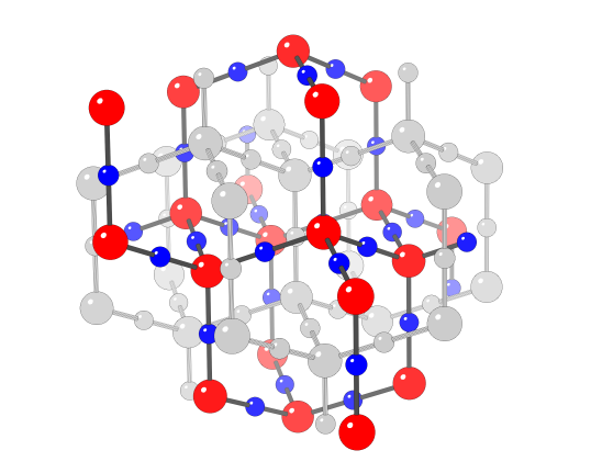
Figure 1: The Cu₂O crystal framework. The structure is shown in ball and stick representation: red atoms are O; blue atoms are Cu. One of the two sublattices is shaded in pale grey for clarity.

Copper oxide, Cu₂O, has NTE at low temperatures. Its coefficient of thermal expansion has been variously measured as having a minimum value between $-$8.0 and $-$2.95 MK^-1 at temperatures between 80 and 100 K, before increasing to become weak positive thermal expansion above 200 K.White (1978); Schäfer and Kirfel (2002); Dapiaggi et al. (2003); Chapman and Chupas (2009)

Cu₂O is also one of the simpler NTE-exhibiting frameworks,Fornasini et al. (2009) its structure consisting of two interpenetrating diamondoid cristobalite lattices—see Figure 1. Despite its structural simplicity compared to other NTE frameworks, the atomic-scale origin of the NTE in Cu₂O is not fully understood.

Inelastic neutron scattering,Bohnen et al. (2009) Raman scattering and luminescenceReimann and Syassen (1989) as well as ab-initio calculationsBohnen et al. (2009); Gupta et al. (2013) have identified specific phonon modes responsible for driving NTE in Cu₂O. All such modes exist below 5 THz, with the largest contribution coming from transverse acoustic modes in the $\Gamma$–X–M region of reciprocal spaceBohnen et al. (2009); Gupta et al. (2013) (in this paper we use the notation of Bradley and CracknellBradley and Cracknell (1972) to label the high-symmetry points of the reciprocal cell). Optic modes that contribute weakly to both NTE and positive thermal expansion (PTE) also exist in this energy range.Reimann and Syassen (1989); Bohnen et al. (2009); Gupta et al. (2013)

A common mechanism for NTE suggested for framework materials is the ‘tension effect’,Barrera et al. (2005) in which transverse vibrations of bridging atoms in a three-atom connection bring the two end atoms towards each other due to the relatively high energy cost of stretching interatomic bonds. Romao et al. (2013); Miller et al. (2009); Sleight (1998) However, there is a similar mechanism in which a group of atoms rotate as a whole and bring inwards the planes of atoms connected to their ends. Both mechanisms are shown in Figure 2. A similar mechanism is found to be important in the related NTE material Zn(CN)₂.Fang et al. (2013) Both types of motions will be correlated and described in terms of phonon normal modes. For zero wave vector, the traditional tension mechanism will be described by optic phonons, but the rotational motion will more likely be part of a transverse acoustic phonon that generates a shear deformation of the structure.

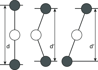
Figure 2: Illustration of two transverse vibrations that can contribute to NTE. Both lead to negligible stretching of nearest-neighbour bonds, but result in reduction of the inter-atomic or inter-planar distances (in this case reducing distance $d$ to $d^{\prime}$). If enough of these vibrations exist with large enough amplitude in a material, they can drive macroscopic NTE.

All materials undergo some drive towards PTE due to longitudinal bond expansion arising from the anharmonicity of interatomic potentials.Dove (1993) However, if a tension-effect mode has low enough energy and thus large enough amplitude (given that a phonon’s amplitude is inversely proportional to the square of its frequencyDove (1993)) and if it comprises sufficiently large a fraction of the full phonon spectrum, then the PTE is outweighed and the net outcome is macroscopic NTE.Miller et al. (2009)

Parametrised potential calculationsMittal et al. (2007) have identified an optic phonon that dominates the low energy density of states. Analysis of its eigenvectors at the $\Gamma$ pointMittal et al. (2007); Sanson (2011) show this mode to consist of rotations of undeformed OCu₄ tetrahedra. This is a type of tension effect known as a rigid unit modeHammonds et al. (1996) (RUM), an established NTE mechanism in some silicate minerals.Heine et al. (1999); Welche et al. (1998) The same mechanism has also been proposed as a result of evidence from neutron powder diffractionSchäfer and Kirfel (2002) where anisotropy of Cu thermal displacement parameters points to significant Cu motion transverse to the $\langle 111\rangle$ directions.

Meanwhile EXAFS work,Chapman and Chupas (2009); Fornasini et al. (2009, 2008, 2007, 2006); Sanson et al. (2006) as well as X-rayChapman and Chupas (2009) and neutronDapiaggi et al. (2008) PDF studies, have led to proposals of an alternative tension effect mechanism involving significant OCu₄ tetrahedral deformations, either in addition to the RUM Chapman and Chupas (2009) or replacing it.Sanson (2009); Sanson et al. (2006) This is due to observations of both expansion and contraction in average Cu$\cdots$Cu distance as a function of increasing temperature, interpreted as deformations of the OCu₄ tetrahedral units.

However, no proposed mechanism has been tested against the known NTE phonons in Cu₂O. It is not enough to determine that a type of large amplitude structural deformation (and therefore possible tension effect mechanism) takes place in the system; in order to understand the driving force behind its NTE, we must find the specific type of tension effect (if any) that corresponds to its NTE-driving modes.

Our approach to this problem is to map phonons from different models of Cu₂O structural flexibility onto those from high quality ab-initio calculations. By observing the degree to which each flexibility model is able to describe the real system’s NTE modes we can thus determine the type of framework flexibility, and the particular manifestation of the tension effect, that drives the NTE in Cu₂O.

II Methods

II.1 Ab-initio lattice dynamics

Table 1: Cu₂O equilibrium cell parameters, as obtained through calculation and experiment. Our value of $a=4.358$ Å is a $\sim$2% overestimation of the experimentally-derived values, a typical result for GGA calculations. The symbol † indicates that the measurements were performed at 300 K. The symbol ‡ indicates that the measurements were performed at 15 K.

Source	a0 / Å
This work (PBE+pseudopotentials)	4.358
PBE+pseudopotentialsCortona and Mebarki (2011)	4.359
LDA+pesudopotentialsCortona and Mebarki (2011)	4.221
PBE+mixed-basis pseudopotentialsBohnen et al. (2009)	4.30
All-electron calculationBohnen et al. (2009)	4.32
X-ray powder diffractionSanson et al. (2006)†	4.27014(7)
Neutron powder diffractionSchäfer and Kirfel (2002)‡	4.2763(2)

Density functional theoryHohenberg and Kohn (1964); Kohn and Sham (1965) simulations were performed using the plane-wave pseudopotential methodPayne et al. (1992) as implemented in CASTEP.Clark et al. (2005) The GGA-PBE functionalPerdew et al. (1996, 1997) was used for all calculations.

Troullier-Martins norm-conserving pseudopotentials describing Cu and O were obtained from the ABINIT FHI database.Fuchs and Scheffler (1999); Abi The density mixing procedure, with 20 densities stored in its history, was implemented for SCF minimisation. A plane-wave cutoff energy of 1100 eV and corresponding FFT grid were used to define the basis for the electronic orbitals. To minimise violation of the acoustic sum rule arising from high-frequency components of the GGA XC functional, a grid 2.5 times denser in each direction was used to represent the electron density and potentials. Electronic Brillouin-zone integrals were evaluated using a $12\times 12\times 12$ Monkhorst-Pack grid. In addition, Cu₂O was explicitly defined as a zero-temperature insulator by keeping band occupancies fixed.

Table 2: Cu₂O phonon frequencies at the $\Gamma$ point for the equilibrium Cu₂O cell volume, as obtained through calculation and experiment. Frequencies are in units of cm^-1. Calculated frequencies are within a few percent of values obtained via experiment, a typical result for DFT. The symbol † indicates data obtained via Reference Sanson, 2011.

Study	T2u	Eu	T1u (TO)	T1u (LO)	Bu	F2g	F1u (TO)	F1u (LO)
This work (DFPT calculation)	64	77	139	140	337	489	607	629
DFPT calculationBohnen et al. (2009)†	72	86	147	148	337	496	609	629
All-electron finite displacement calculationSanson (2011)	67	119	142	146	350	515	635	654
Raman+luminescenceReimann and Syassen (1989)	86	110	152	152	350	515	633	662

A geometry optimisation was performed at 0 GPa such that residual stresses on the cell were within 0.02 GPa. Since the atomic coordinates of Cu₂O are fixed by its $Pn\bar{3}m$ symmetry, only the cell parameter required optimisation. Table 1 shows the converged result of $a=4.358$ Å. This is a 2% overestimation of the experimental value, as is typical for GGA-PBE.

Phonons were calculated for a total of six unit cell lengths: at equilibrium as well as values of 4.25, 4.30, 4.35, 4.40 and 4.45 Å. Density functional pertubation theoryRefson et al. (2006) (DFPT) was used with an $8\times 8\times 8$ Monkhorst-Pack phonon wave vector grid that was offset to place one of the grid points at $\Gamma$. Convergence tolerance for force constants during the DFPT calculations was set at 10^-6 eV Å^-2. Long-range electric field effects which lead to LO/TO splitting were accounted for during the calculations and the phonon acoustic sum rule was enforced.

Fourier interpolation was used to generate phonons along high-symmetry directions for the production of dispersion curves, as well as for 6000 wave vectors distributed randomly throughout the Brillouin zone for the production of densities of states. As shown in Table 2, $\Gamma$-point frequencies are within a few percent of values obtained through other calculations and experiments. The final phonon dispersion curves shown in Figure 4 are also a close match for dispersion curves obtained previously through DFT and inelastic neutron scattering.Bohnen et al. (2009); Gupta et al. (2013)

II.2 Grüneisen parameter calculations

The Grüneisen parameter relates the vibrational spectrum of a material to its thermal expansion behaviour. At the macroscopic level, the volumetric coefficient of thermal expansion of a material, $\alpha_{\text{V}}$, can be written asDove (1993)

$$\alpha_{\text{V}}=\frac{\overline{\gamma}C_{V}}{BV}$$ (1)

where $\overline{\gamma}$ is the macroscopic Grüneisen parameter, $C_{V}$ is the heat capacity at constant volume, $B$ is the bulk modulus and $V$ is the system volume. Since $C_{V}$, $B$ and $V$ are constrained to have positive values, the sign of the thermal expansion coefficient $\alpha_{\text{V}}$ is determined by the sign of $\overline{\gamma}$.

At the microscopic level, the mode Grüneisen parameter, $\gamma_{i,\mathbf{k}}$, is given byDove (1993)

$$\gamma_{i,\mathbf{k}}=-\frac{V}{\omega_{i,\mathbf{k}}}\frac{\partial\omega_{i,\mathbf{k}}}{\partial V}$$ (2)

where $V$ is the unit cell volume, $\omega$ the mode frequency, and the indices $i$ and $\mathbf{k}$ refer to an individual phonon by mode and wave vector respectively. $\gamma_{i,\mathbf{k}}$ is normally positive for a given mode, since atomic bonds normally stiffen under compression, thereby increasing phonon frequency. However in some situations, such as for tension-effect modes as described in the Introduction and Figure 2, mode frequency decreases on compression and thus $\gamma_{i,\mathbf{k}}$ is negative.

$\overline{\gamma}$ is calculated by taking the sum of microscopic mode Grüneisen parameter values, $\gamma_{i,\mathbf{k}}$, weighted according to the contribution of each mode to overall heat capacity $C_{V}$.Dove (1993) Therefore, phonons with positive $\gamma_{i,\mathbf{k}}$ contribute to PTE and phonons with negative $\gamma_{i,\mathbf{k}}$ contribute to NTE.

Values of $\gamma_{i,\mathbf{k}}$ were calculated for the $a=4.358$ Å equilibrium structure by considering changes in phonon frequency and volume at $a=4.30$ Å. The result was then converted to a linear colour scale that ranged from red ($\gamma_{i,\mathbf{k}}\leq-8$) to white ($\gamma_{i,\mathbf{k}}=0$) through to blue ($\gamma_{i,\mathbf{k}}\geq+8$).

Plotted dispersion curves were then shaded according to their corresponding value of $\gamma_{i,\mathbf{k}}$ on this scale, whilst bins that made up the plotted density of states were shaded according to the average $\gamma_{i,\mathbf{k}}$ for each bin using the same colour scale. As can be seen in Figure 4, this process allowed for easy identification and comparison of different modes’ contributions to positive and negative thermal expansion.

II.3 Generation of flexibility models

Simple models were devised to investigate flexibility in the Cu₂O framework. Our intention was not to reproduce any other properties of the system other than to abstract the rigid and flexible parts of the framework down to very stiff or complete flexibility. This approach allowed the simulation of different types of tension effect in this material.

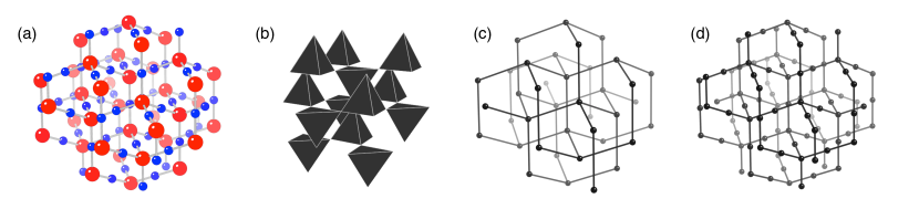
Figure 3: (a) The Cu₂O structure in ball-and-stick representation: red atoms are O, blue atoms are Cu. (b) Representation of Cu₂O Flexibility Model 1, consisting of corner-sharing rigid OCu₄ tetrahedra. (c) Representation of Cu₂O Flexibility Model 2, consisting of rigid O–Cu–O rods: grey spheres represent flexible linkages. (d) Representation of Cu₂O Flexibility Model 3, consisting of rigid Cu–O rods: grey spheres represent flexible linkages.

Our flexibility models were created in the following manner. The equilibrium Cu₂O cell was reconstructed in the program GULP.Gale and Rohl (2003) A two-body harmonic potential was applied to the Cu–O bond and three-body harmonic potentials were applied to Cu–O–Cu and O–Cu–O bonds. All atoms were assigned zero charge whilst equilibrium bond lengths and angles were chosen such that the cell would remain unchanged upon a zero pressure geometry optimisation.

We were able to control the rigid and flexible regions of the model by changing the force constants in this setup. For this study the force constant for the two-body potential was fixed at 100 eV Å^-2 to model a stiff Cu–O bond. The force constants for the three-body potentials were set to either 100 eV rad^-2 or zero, depending on whether the flexibility model in question required those bond angles to be fixed or to vary freely.

Flexibility models considered were:

1. Rigid OCu₄ tetrahedra wherein Cu–O–Cu bond angles were fixed whilst O–Cu–O bond angles could vary freely.

2. Rigid CuO₂ rods wherein O–Cu–O bond angles were fixed whilst Cu–O–Cu bond angles could vary freely.

3. Rigid CuO rods wherein both O–Cu–O and Cu–O–Cu bond angles could both vary freely.

All of these models are illustrated in Figure 3. It can be seen in this diagram that Model 1 corresponds to rigid OCu₄ tetrahedra; Model 2 to rigid O–Cu–O rods and Model 3 to rigid Cu–O rods. In addition, it should be noted that Model 1 and Model 2 are constrained versions of Model 3. An even further constrained model, where both O–Cu–O and Cu–O–Cu bond angles were fixed, was discounted as this would not have any free deformations and thus could not correspond to any type of tension effect.

Phonons were calculated for all three flexibility models at the same wave vectors as in the ab-initio dispersion curves and densities of states. Zero-frequency solutions corresponded to modes involving free deformations of the model structure, whilst solutions with non-zero frequency corresponded to modes that violated the constraints of that model (e.g. Cu–O–Cu bond bending in Model 1).

II.4 Mapping of flexibility model phonons onto ab-initio phonons

Table 3: Cu₂O equilibrium elastic and bulk moduli, as obtained through calculation and experiment. In order to account for scatter present in the elastic modulus data as calculated from acoustic modes close to the $\Gamma$ point, values and errors presented here are interpolated from a straight line fit through data points obtained from each volume. Moduli are in units of GPa. Calculated values are close to values obtained via experiment. The symbol * indicates that, whilst no B₀ value was quoted in the original paper, it was inferred here using Equation 4. The symbol † indicates that the experiments were performed at room temperature. The symbol ‡ indicates that the experiments were performed at 4 K.

Source	$c_{11}$	$c_{12}$	$c_{44}$	B0
This work (PBE+pseudopotentials)	$114.5\pm 0.9$	$87\pm 3$	$7.2\pm 0.7$	$96\pm 4$
PBE+pseudopotentialsCortona and Mebarki (2011)	116	100	8	106
Inelastic neutron scatteringBeg and Shapiro (1976)†	$126.1\pm 1.2$	$108.6\pm 0.4$	$13.6\pm 11.4$	$114.4\pm 1.3$*
Ultrasonic interferometryManghnani et al. (1974)†	$122.88\pm 0.38$	$106.50\pm 0.71$	$12.10\pm 0.30$	$111.96\pm 0.27$
Pulse echoHallberg and Hanson (1970)‡	121	105	10.9	105.7

For each ab-initio phonon mode at each wave vector a ‘match’ value, $m_{i,\mathbf{k}}$, was defined as

$$m_{i,\mathbf{k}}=\sum_{j}\frac{\mathbf{e}_{i,\mathbf{k}}\cdot\mathbf{e}_{j,\mathbf{k}}}{\Omega^{2}+\omega^{2}_{j,\mathbf{k}}}$$ (3)

where $\mathbf{e}$ is an eigenvector, $\omega$ is a phonon frequency, the index $i$ denotes a mode in the ab-initio calculation, the index $j$ denotes a mode in a given flexibility model and the index $\mathbf{k}$ denotes a phonon wave vector. $\Omega$ is an arbitrary scale factor that helps avoid divide-by-zero errors; we set it equal to 1 THz so that a $\omega^{2}_{j,\mathbf{k}}$ value of 0 gave a $1/(\Omega^{2}+\omega^{2}_{j,\mathbf{k}})$ value of 1 THz^-2.

$m_{i,\mathbf{k}}$ represents the degree to which the flexibility model in question is able to reproduce the mode $i$ at the wave vector $\mathbf{k}$. Scaling by $\Omega^{2}+\omega^{2}_{j,\mathbf{k}}$ ensured that only flexibility model modes with zero or close-to-zero frequency contributed to $m_{i,\mathbf{k}}$, as discussed in Section II.3 above.

Due to the normalisation and orthogonality of the eigenvectors, each $m_{i,\mathbf{k}}$ has a value between 0 and 1. A value of 0 indicates that the flexibility model could not reproduce the ab-initio mode eigenvector $i$ at all, whilst a value of 1 indicates a perfect match.

A full set of $m_{i,\mathbf{k}}$ were computed for the equilibrium Cu₂O structure. As with the $\gamma_{i,\mathbf{k}}$ plots, $m_{i,\mathbf{k}}$ values were then converted to a linear colour scale. This ranged from white ($m_{i,\mathbf{k}}=0$) through to black ($m_{i,\mathbf{k}}=1$). Plotted ab-initio dispersion curves were shaded according to their corresponding value of $m_{i,\mathbf{k}}$ and densities of states were shaded according to the average $m_{i,\mathbf{k}}$ for each bin.

As seen in Figure 4, this approach yields a convenient visual representation of which real system phonons are reproduced by each flexibility model. This highlights the different types of tension effect-related deformation present in the full phonon spectrum.

II.5 Elastic modulus calculations

Acoustic phonon modes with negative $\gamma_{i,\mathbf{k}}$, present in Cu₂O,Bohnen et al. (2009); Gupta et al. (2013) are indicative of elastic softening. Changes in the elastic moduli could therefore be tracked by monitoring the softening of acoustic modes as a function of pressure.Dove (1993)

A dynamical matrix solely for the acoustic modes was constructed for all six simulated cells. Monte Carlo minimisation was then used to fit elastic modulus tensor values to both the acoustic dynamical matrix and to the original ab-initio acoustic phonon frequencies. The bulk modulus for the equilibrium cell was also calculated using the cubic cell formulaHill (1952)

$$B=\frac{c_{11}+2c_{12}}{3}$$ (4)

where $B$ is the bulk modulus and $c_{ij}$ are the $i$,$j$^th components of the elastic modulus tensor.

Elastic moduli and bulk moduli for the equilibrium cell, compiled in Table 3, are a good match for other data obtained through theory and experiment.

III Results

III.1 Thermal expansion in Cu₂O

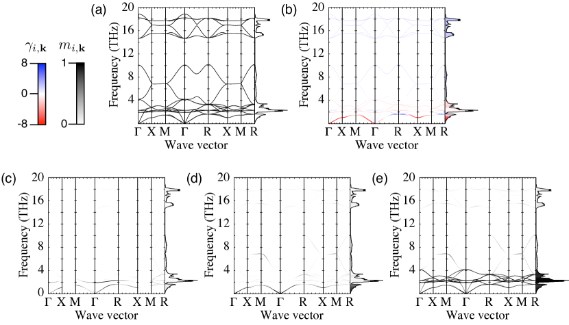
Figure 4: (a) Phonon dispersion curves and full Brillouin zone density of states for the equilibrium Cu₂O cell. We use the notation of Bradley and CracknellBradley and Cracknell (1972) to label special points in reciprocal space: $\Gamma=(0,0,0)$, $\text{X}=(0.5,0,0)$, $\text{M}=(0.5,0.5,0)$, and $\text{R}=(0.5,0.5,0.5)$. Eigenvector matching was employed to differentiate crossings and anti-crossings in the dispersion curves. (b) Shows the same data shaded according to the value of $\gamma_{i,\mathbf{k}}$ of each mode at each wave vector with respect to phonons calculated for a Cu₂O cell of $a=4.30$ Å. The colour scale ranges from red ($\gamma_{i,\mathbf{k}}\leq-8$) to white ($\gamma_{i,\mathbf{k}}=0$) through to blue ($\gamma_{i,\mathbf{k}}\geq+8$). Bins that make up the density of states are shaded according to the average $\gamma_{i,\mathbf{k}}$ for each bin using the same colour scale. (c), (d) and (e) Show the same data shaded according to the value of $m_{i,\mathbf{k}}$ of each mode at each wave vector. The colour scale ranges from white ($m_{i,\mathbf{k}}=0$) through to black ($m_{i,\mathbf{k}}=1$). Bins that make up the densities of states are shaded according to the average value of $m_{i,\mathbf{k}}$ for each bin using the same colour scale. (c) Shows $m_{i,\mathbf{k}}$ values for Flexibility Model 1, (d) Shows $m_{i,\mathbf{k}}$ values for Flexibility Model 2, (e) shows $m_{i,\mathbf{k}}$ values for Flexibility Model 3.

Equilibrium cell phonons, their associated mode Grüneisen parameters and flexibility model match values are all shown in Figure 4. The results are a close match to previous calculations and experimental data.Bohnen et al. (2009); Reimann and Syassen (1989); Gupta et al. (2013) The largest contribution to NTE in the 0–5 THz range comes from the transverse acoustic modes in the $\Gamma$–X–M region of reciprocal space ($\gamma_{i,\mathbf{k}}\sim-9$ for $\Gamma$ to X and their surroundings, slowly rising towards $-3$ approaching M). There is also some small contribution from several optic modes spanning the Brillouin zone in the 2–5 THz range ($\gamma_{i,\mathbf{k}}\sim-1$). The largest contribution to PTE in the 0–5 THz range comes from the three acoustic modes around R ($\gamma_{i,\mathbf{k}}\sim+5$) There is also some very small contribution around $\Gamma$ from the longitudinal acoustic mode and a pair of optic modes ($\gamma_{i,\mathbf{k}}\sim+2$).

Model 1, consisting of rigid OCu₄ tetrahedra, is a reasonable match for some NTE and PTE modes but not for others, suggesting there is limited correlation between thermal expansion and modes available to this model. The main good match is for a single, nearly dispersionless, weak NTE optic mode at $\sim 2$ THz that exists throughout most of the Brillouin zone. This is a moderate match to a RUM consisting of OCu₄ tetrahedral rotations and has a particularly strong match in the $\Gamma$–R direction. The same optic mode is also a very weak match for Model 2 (rigid CuO₂ rods) but a strong match for Model 3 (which is a less constrained version of Model 1, in that is allows Cu–O–Cu bond bending). We conclude that, away from the $\Gamma$-R region, the mode is forced to undergo some Cu–O–Cu bond bending as a result of constraints of the Cu₂O structure and connectivity as well as phonon wave vector—this point is discussed in greater depth in Section IV.1. There is therefore some small contribution to NTE from rotations of rigid or near-rigid OCu₄ tetrahedra.

Model 2, consisting of rigid O–Cu–O rods, is a strong match to the principal NTE modes highlighted in Figure 4. The NTE in Cu₂O is therefore primarily driven by vibrations of rigid O–Cu–O rods. Weak NTE optic modes that do not match Model 1 are also moderate matches for Model 2. Again, as these modes are also a strong match for Model 3, it follows that the remaining NTE modes are almost a match for Model 2, but are forced to undergo some O–Cu–O bond bending for the same reasons as stated above for Model 1. There is therefore also some small contribution to NTE from motion of near-rigid O–Cu–O rods.

Finally Model 3, consisting of rigid CuO rods, dominates the low energy region of the phonon spectrum, confirming that Cu–O bond stretching is a high energy process. Since the NTE-driving modes described by this model can also be described by Model 1 or Model 2, the extra flexibility afforded to Model 3 (compared the others) does not offer any additional tension effect that leads to NTE in Cu₂O.

Putting everything together, we can describe the thermal expansion of Cu₂O in terms of its vibrational spectrum as follows: the 0–1 THz range is dominated by strong NTE modes in the $\Gamma$-X-M region of the Brillouin zone. These correspond to vibrations of rigid O–Cu–O rods. At $\sim 1.8$ THz there is a strong PTE contribution from modes at and around the R point. This is expected for structures consisting of a pair of interpenetrating lattices: the R point corresponds to $\Gamma$ for an individual sublattice, and acoustic modes here correspond to the sublattices moving in anti-phase.

At $\sim 2$ THz there is a nearly dispersionless weak NTE mode that spans the entire Brillouin zone and thus forms the large and sharp peak in the low energy phonon density of states. This mode corresponds to rotations of rigid OCu₄ tetrahedra where wave vector allows and to near-rigid OCu₄ tetrahedra where constraints of framework connectivity and wave vector mean rigid unit rotations are not possible. Weak PTE modes around $\Gamma$ also exist in this frequency range; these correspond to rigid Cu–O rod motion and no particular tension effect.

At $\sim 3$–4 THz there is a second band of weak NTE modes that also span much of the Brillouin zone, but with a greater dependence of frequency on wave vector than the $\sim 2$ THz mode. These modes correspond to motions of near-rigid O–Cu–O rods.

Higher frequency modes involve a non-trivial level of Cu–O bond stretching and thus contribute to standard PTE.

III.2 A predicted phase transition

Softening of the NTE phonon modes as a function of pressure is illustrated in Figure 5. Zone-centre softening of acoustic branches along $\Gamma$–X corresponds to instabilities in the elastic moduli $c_{44}$ and $c_{11}-c_{12}$ which would, in turn, drive a proper ferroelastic phase transition.Dove (1993)

Figure 6 shows elastic moduli for all six calculated volumes as a function of effective pressure. The plot shows faster softening in $c_{44}$, indicating a transition to an orthorhombic phaseDove (1993) at $6.0\pm 0.8$ GPa.

Figure 5: Phonon dispersion curves and full Brillouin zone density of states for Cu₂O with unit cell parameter $a=4.25$ Å  corresponding to an effective pressure of 9.6 GPa. We use the notation of Bradley and CracknellBradley and Cracknell (1972) to label special points in reciprocal space: $\Gamma=(0,0,0)$, $\text{X}=(0.5,0,0)$, $\text{M}=(0.5,0.5,0)$, and $\text{R}=(0.5,0.5,0.5)$. Eigenvector matching was employed to differentiate crossings and anti-crossings in the dispersion curves. The $\Gamma$–X acoustic NTE mode is completely soft at this pressure.

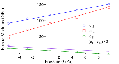
Figure 6: The elastic moduli of Cu₂O as a function of pressure. Straight line fits have been applied to the data for each modulus. $c_{44}$ and $c_{11}-c_{12}$ both soften as a function of pressure. $c_{44}$ reaches zero before $c_{11}-c_{12}$, indicating a ferroelastic phase transition to an orthorhombic structure at $6.0\pm 0.8$ GPa.

In order to characterise the new phase, another geometry optimisation was carried out on the $a=4.25$ Å unit cell under an applied hydrostatic pressure of 8.5 GPa and using the convergence criteria detailed earlier in Section II.1. On this occasion, however, only $P1$ symmetry was applied (though 90^∘ cell angles remained fixed). In addition, one cell parameter was changed to 4.26 Å and the fractional coordinate of O at $(0,0,0)$ was changed to $(0.02,0,0)$. These minor adjustments ensured the geometry optimiser did not become trapped at an energy maximum.

The relaxed cell was confirmed as orthorhombic with space group $Pnnn$. Fractional coordinates of the cell contents remained unchanged from their values in the cubic cell, however the cell parameters at 8.5 GPa became $a=4.256$ Å, $b=4.261$ Å and $c=4.263$ Å.

IV Discussion

IV.1 Framework flexibility and NTE in Cu₂O

We now understand the driving force behind NTE in Cu₂O. It is dominated by low frequency rigid O–Cu–O rod motion, which corresponds to the translational acoustic modes spanning the $\Gamma$–X–M region of reciprocal space. There is some small additional contribution at higher frequencies from rigid and near-rigid OCu₄ tetrahedral rotation as well as near-rigid O–Cu–O rod motion, all corresponding to optic modes throughout the Brillouin zone.

The O–Cu–O rigid rod mechanism goes beyond the traditional picture of a tension effect. Instead of transverse vibrations of individual bonds (as illustrated earlier in Figure 2) the mechanism consists of rotations of rigid rods made up of multiple atoms. As these rods rotate they necessarily pull atomic planes together and this motion drives macroscopic NTE.

The NTE in Cu₂O can therefore be described as being driven by RUMs, but with the rigid unit recast as an O–Cu–O rod. The additional NTE modes would then be O–Cu–O quasi-RUMsHammonds et al. (1996) (QRUMs—modes close to being RUMs but which involve some small deformation of a rigid unit due to constraints of framework structure, connectivity and of wave vector), as well as both RUMs and QRUMs of an OCu₄ tetrahedral unit.

That NTE in Cu₂O is primarily driven by a mode that involves significant deformation of OCu₄ tetrahedra had previously been proposed.Sanson (2009); Sanson et al. (2006); Chapman and Chupas (2009) However, this study marks the first time that any proposed mechanisms have been tested against eigenvectors of confirmed NTE modes throughout the Brillouin zone. Furthermore, these previously proposed mechanisms all assumed a Cu–O bond as the basic rigid unit; our work instead shows that an O–Cu–O rigid rod is in fact the fundamental rigid unit as far as NTE behaviour in this material is concerned.

Our analysis of the vibrational spectrum therefore also provides insight into the intrinsic framework flexibility of Cu₂O. As known previously,Sanson et al. (2006) Cu–O bond stretching is a high energy process and this is also evident in our analysis, as Cu–O bond stretching modes have been shown to exist only at frequencies greater than 4 THz.

The lowest energy deformations (0–1 THz) of the structure are, however, RUMs involving rigid O–Cu–O rods. O–Cu–O bond angle bending does not occur until we reach optic modes at slightly higher frequencies $\geq 2$ THz. There is therefore some small, but not trivial, cost to bending the O–Cu–O bond. This is, perhaps, not surprising given the particularly high sensitivity to bond geometry associated with bonds involving d orbitals—as is the case for the Cu centre of the O–Cu–O rod.

Meanwhile, one $\sim 2$ THz optic mode consists of either OCu₄ RUMs (along $\Gamma$–R) or OCu₄ QRUMs (the rest of the Brillouin zone), again as a result of constraints of the framework structure and connectivity as well as wave vector. Cu–O–Cu bond bending has minimal effect on the mode frequency—hence the size of the peak in the phonon density of states at this frequency. There is therefore minimal energy cost to Cu–O–Cu bond bending.

IV.2 Comparison with other NTE materials

The dominant NTE mode in Cu₂O is reminiscent of the mechanism driving weak low-temperature NTE in simple frameworks with a diamond or zincblende lattice such as Si, Ga and CuCl.White (1993) NTE in these materials is driven by translational acoustic vibrations exactly like those of the rigid O–Cu–O rod model. This is not surprising given that Model 2 is effectively a pair of interpenetrating diamondoid lattices. Unlike the aforementioned materials however, Cu₂O has greater structural flexibility due to the possibility of bending the O–Cu–O bond and thus has additional, albeit weak, NTE mechanisms available to it.

Zn(CN)₂, another material composed of two interpenetrating diamondoid lattices, might therefore be expected to behave in a similar fashion to Cu₂O. Like Cu₂O, NTE in Zn(CN)₂ is driven primarily by transverse acoustic modes with some smaller contribution from optic modes.Fang et al. (2013) However, whilst the acoustic modes in question are reminiscent of the O–Cu–O acoustic modes in Cu₂O (in that they minimise deformation of the Zn–N–C–Zn rod), in practice some minimal deformation of the rod must take place as deformation of the Zn(C/N)₄ tetrahedral unit in Zn(CN)₂ is a high frequency process. In addition, the dominant NTE-driving acoustic mode in Zn(CN)₂ spans the entire Brillouin zone, whilst the dominant acoustic NTE mode in Cu₂O only spans the $\Gamma$–X–M region of reciprocal space. This, in turn, means that the NTE in Zn(CN)₂ is much largerGoodwin and Kepert (2005) ($\alpha_{\text{linear}}=-16.9$ MK^-1), a difference that can be attributed to the CN bridges in Zn(CN)₂ giving its framework more overall degrees of freedom than Cu₂O.Goodwin (2006)

IV.3 On the use of flexibility model mapping

The approach taken in this study, whereby phonon eigenvectors generated from simple flexibility models are mapped onto full ab-initio calculated modes, has enabled identification of modes in Cu₂O that correspond to different types of structural deformation. This, in turn, has allowed for insightful evaluation of proposed NTE mechanisms.

We have found this approach to be more efficient and less error-prone than relying on visual inspection of modes of interest. It has proven useful, in particular, when differentiating Cu₂O modes that have very different features but exist at similar energies; such as in the crowded 2–5 THz range of the phonon spectrum.

We anticipate that this same approach will prove highly useful in the analysis of framework flexibility and tension effect-driven NTE in more complex systems such as metal-organic frameworks.Rao et al. (2008) These materials, a number of which exhibit NTE,Rowsell et al. (2005); Wu et al. (2008) have unit cells typically comprising hundreds of atoms in addition to complex internal bonding. As a result, a full analysis of their dispersion curves using more conventional methods would be a highly complex process.

IV.4 High-pressure phase transitions

Given that negative Grüneisen parameter indicates mode softening as a function of pressure,Dove (1993) one could argue that NTE itself is an outcome of the drive towards a displacive phase transition at pressure. In this case, our results predict a transition to an orthorhombic phase at $6.0\pm 0.8$ GPa driven by the strongest NTE modes at $\Gamma$–X. However, in practice, there are numerous conflicting reports of high-pressure phase transitions of Cu₂O.

At low temperatures Cu₂O is in fact metastable above $\sim 4$ GPa,Sinitsyn et al. (2004); Machon et al. (2003) decomposing at equilibrium to form CuO and Cu. Some have predicted a displacive phase transition on the basis of the existence of phonon soft modes Kalliomäki et al. (1979) as well as measuredManghnani et al. (1974) and calculatedCortona and Mebarki (2011) softening in $c_{44}$ and $c_{11}-c_{12}$. Ab-initio calculations on strained Cu₂O cellsCortona and Mebarki (2011) are a close match to our results and show $c_{44}$ softening fastest, predicting a shear instability at $\sim 8$ GPa. A transition was observed experimentally at 5 GPaKalliomäki et al. (1979) using X-ray powder diffraction and a diamond anvil cell. However it was not possible to conclusively identify the new phase at that time.

On the other hand, further X-ray diffraction diamond anvil cell experiments have found no displacive phase transition in the 0–10 GPa range. In one studyWerner and Hochheimer (1982) the cubic structure was observed as remaining intact until a known higher-pressure phase transition to a hexagonal structure at 10 GPa. In another studySinitsyn et al. (2004) the sample was observed to amorphise at pressure before transforming to the same hexagonal phase at 11 GPa.

Another set of similar experiments did find a displacive transition, but at 0.6Webb et al. (1990) or 0.7–2.2 GPa,Machon et al. (2003) much smaller pressures than our prediction. This transition was observed to be proper ferroelastic in nature and the new phase was identified as tetragonalMachon et al. (2003) as opposed to our prediction of an orthorhombic phase. Curiously, the structure was also observed to transform into a pseudocubic phase at  8.5 GPa.Machon et al. (2003)

These inconsistencies can partly be attributed to the fact that phase transitions observed experimentally in Cu₂O at high pressure are known to be highly sensitive to the experimental environment, especially the hydrostaticity of the pressure medium.Kalliomäki et al. (1979); Machon et al. (2003) Furthermore significant peak broadening under pressure obscures any peak splitting,Machon et al. (2003) making pressure-induced displacive transitions in Cu₂O difficult to observe experimentally.

Another factor which can complicate the identification of the new phase is the fact that changes in the unit cell for displacive transitions are usually minute. In our predicted orthorhombic phase, the $b$ and $c$ parameters were found to be especially close, within 0.05% of one another. Such a minute difference may explain why a tetragonal phase is sometimes observed in experiments whilst we predict an orthorhombic structure.

V Conclusions

A full analysis of the NTE mechanism in Cu₂O was conducted. This was achieved by mapping different structural flexibility models onto results from ab-initio lattice dynamics calculations. The degree to which each model could match the ab-initio phonons determined how well it could describe specific modes in the real system.

It was found that NTE in Cu₂O is dominated by low frequency vibrations of rigid O–Cu–O rods. There is also some smaller contribution at higher frequency from rigid and near-rigid OCu₄ tetrahedral rotation and near-rigid O–Cu–O rod motion.

It was also found that the primary NTE mode drives a proper ferroelastic phase transition at high pressure. Our simulations predict this to be to an orthorhombic structure with space group $Pnnn$.