Spin-orbit coupling as a source of long-range triplet proximity effect in superconductor-ferromagnet hybrid structures

Abstract

We investigate the proximity effect in diffusive superconducting hybrid structures with a spin-orbit (SO) coupling. Our study is focused on the singlet-triplet conversion and the generation of long-range superconducting correlations in ferromagnetic elements. We derive the quasiclassical equations for the Green’s functions including the SO coupling terms in form of a background SU(2) field. With the help of these equations, we first present an interesting complete analogy between the spin diffusion process in normal metals and the generation of the triplet components of the condensate in a diffusive superconducting structure in the presence of SO coupling. From this analogy it turns out naturally that the SO coupling is an additional source of the long-range triplet component (LRTC) besides the magnetic inhomogeneities studied in the past. This analogy opens a range of possibilities for the generation and manipulation of the triplet condensate in hybrid structures. In particular we demonstrate that a normal metal with a SO coupling can be used as source of LRTC if attached to a S/F bilayer. We also demonstrate an explicit connection between an inhomogeneous exchange field and SO coupling mechanisms for the generation of the LRTC and establish the conditions for the appearance of the LRTC in different geometries. Our work gives a global description of the singlet-triplet conversion in hybrids structures in terms of generic spin-fields and our results are particularly important for the understanding of the physics underlying spintronic devices with superconductors.

I Introduction

It is by now common knowledge that the interaction between conventional superconductivity and ferromagnetism in superconductor-ferromagnet (S/F) hybrids leads to a new type of superconducting correlations in a triplet stateBergeret2001 ; BergeretRMP . Since the prediction of this intriguing phenomenon in 2001, there has been an increasing experimental activity in the field.Keizer2006 ; Birge2010 ; Robinson2010 ; Robinson2010b ; Leksin2012 ; Witt2012 ; Wang2012 ; Robinson2012 ; Chiodi ; Pal2014 ; Robinson2014 ; Kalchemin ; Banerjee ; Aarts2010 ; Wang2010 ; Sprungmann2010 ; Usman2011 ; Birge2012 ; Villegas2012 ; Aarts2012 ; Yates2013 That research focuses mainly on the creation and control of superconducting triplet correlations in hybrid structures with the ultimate goal of using polarized spin supercurrents in spintronic devices.EschrigPT To achieve this, it is essential to identify the optimal material combination and hence it is of fundamental interest to understand the physics that underpin triplet generation.

In S/F structures, superconducting correlations can penetrate into the ferromagnetic metal due to the proximity effect. If the ferromagnet is a monodomain magnet, the superconducting condensate consists of two components: the usual singlet one and the triplet component with total zero spin-projection with respect to the magnetization axis of the F layer. In a diffusive system both components decay over a short distance given by $\sqrt{D/h}$, where $D$ is the diffusion coefficient of the F layer and $h$ the exchange field. If, however, the triplet components with finite total spin are generated, these can penetrate the F region over a much longer distance of the order of $\sqrt{D/2\pi T}$.

It is commonly believed that singlet-long-range triplet (in short singlet-triplet) conversion happens only in the presence of magnetic inhomogeneities, as for example magnetic domain walls,Bergeret2001 ; Fominov2007 ; Volkov2008 ; Kupferschmidt2009 ; Buzdin2011 ferromagnetic multilayers with different magnetization orientationsBergeret2003 ; Houzet2007 ; Halterman2008 , or interfaces with magnetic disorder.Eschrig2008 ; Linder2009 Such inhomogeneities presumably explain the observation of long-ranged Josephson currents through Ho-Co-Ho bridges, due to the spiral-like magnetization of the Ho layersRobinson2010 , or though ferromagnetic X-Co-X multilayers, where the inhomogeneous magnetization of X=PdNi,CuNi, Ni might act as spin-mixersBirge2010 ; Birge2012 More surprising is the observation of a long-range Josephson effect in lateral structures based on the half-metallic CrO₂.Keizer2006 ; Aarts2010 ; Aarts2012 A first explanation for such observations assumes a spin-active interface between the CrO₂ layer and the superconductor, consequence of a magnetic inhomogeneity at the atomic level.Eschrig2008

In ballistic heterostructures it has been shown that spin-orbit (SO) coupling can also be a source for a triplet superconducting condensate.Edelstein2003 ; Duckheim2011 ; Takei2012 ; Takei2013 ; jain0 Being anisotropic in momentum this condensate component is very sensitive to disorder and vanishes in diffusive systems. However, in a recent work we have demonstrate that in S/F diffusive systems a finite spin-orbit (SO) coupling can be also a source for the s-wave long-range triplet correlations (LRTC).BT2013 A finite SO coupling can result from either an intrinsic property of materials without inversion symmetrySamokhin2009 or from geometrical constraints such as low dimensional structures or interfaces between different materials.Rashba ; Edelstein2003 ; Koroteev2004 ; Ast2007 ; Miron2010 ; Linder2011 ; Duckheim2011 ; Takei2012 ; Takei2013 Specifically, Ref. BT2013 presented a unified view of the singlet-triplet conversion which connects the magnetic inhomogeneous mechanism with the one based on SO coupling.

In the present work we readdress the problem of singlet-triplet conversion in diffusive S/F structures in the presence of arbitrary (linear in momentum) spin-orbit coupling and go a step further. The main goal of the present paper is twofold: First, we present a complete analogy between the diffusion of a spin density in a normal metal and the singlet-triplet conversion in superconducting hybrids. This analogy opens a new view of the singlet-triplet conversion that helps in the understanding of the proximity effect in more complex hybrid structures. Second, we present the derivation of quasiclassical equations in the presence of a SO-coupling and superconducting correlations. These equations can be very useful not only to describe the singlet-triplet conversion but also for the study of the dynamics of S/F hybrids. With the help of these equations we analyze different hybrid structures and discuss the condition for the singlet-triplet conversion. In particular we show that all triplet components can be generated in a S/F/N structure, provided the conductor N exhibits a SO coupling. We also show that while for a transverse multilayer structure of S/F/S type, the ”old” picture of magnetic inhomogeneities can explain the long-range Josephson couplingBirge2010 ; Robinson2010 , in lateral S/F structures the SO mechanism may be consider as the main mechanism for singlet-triplet conversion.Keizer2006 ; Aarts2010

The structure of the paper is the following: In the next section we review the spin diffusion in the normal case. We discuss the spin diffusion and relaxation in a normal metal in the presence of a generic SO coupling, placing emphasis on the main mechanism that can change the direction of the spin. In section III.1 we discuss the singlet-triplet conversion in a proximity metal with SO coupling and draw an analogy between the singlet-triplet conversion and the ”precession” of the spin density in the normal state. In section III.2 we readdress the original problem of singlet-triplet conversion in a Bloch domain wallBergeret2001 and show that it is gauge-equivalent to the one of a ferromagnet with a homogeneous exchange field and SO coupling. In the previously mentioned sections we base our analysis on a heuristic SU(2) covariant diffusion equation. A rigorous derivation of the quasiclassical kinetic equation for the Green function is presented in section IV. We present both non-equilibrium (Keldysh), and equilibrium (Matsubara) formalisms. In section V we discuss hybrid structures of different geometries. We show that the triplet component with a finite total spin can be generated in a S/F/N structure with a homogeneous magnetized F, provided SO coupling in the N metal. We also analyze a transversal and longitudinal S/F structure and demonstrate that even in the case of a homogeneous magnetization, an interfacial SO coupling can generate long-rang correlations. Finally we present some discussions and a summary of results in our concluding section.

II Spin diffusion and relaxation in normal systems with spin-orbit coupling

To understand how SO coupling can affect the proximity effect in S/F systems, it is instructive to recall the physics of spin diffusion in a normal system. For this sake we consider a normal conductor described by the Hamiltonian

$$H_{0}=\frac{{\bf p}^{2}}{2m}-\frac{1}{2}\Omega^{a}({\bf p})\sigma^{a}+V_{imp}$$ (1)

where $V_{imp}$ is the spin-independent potential of randomly distributed impurities, and the second term, $H_{SO}=\frac{1}{2}\Omega^{a}({\bf p})\sigma^{a}$ with $\Omega^{a}({-\bf p})=-\Omega^{a}({\bf p})$, describes a generic SO coupling allowed in any system with lack of inversion symmetry. The matrices $\sigma^{a}$, with $a=x,y,z$, are the Pauli matrices. Physically, the above SO coupling corresponds to an effective momentum-dependent Zeeman field which induces precession of the electron spin about the direction of the vector ${\bm{\Omega}}({\bf p})=\{\Omega^{x}({\bf p}),\Omega^{y}({\bf p}),\Omega^{z}({\bf p})\}$.

In this work we consider spin dynamics in the diffusive limit, i. e. when the elastic mean free path $l=\tau v_{F}$ (here $\tau$ is the momentum relaxation time and $v_{F}$ is the Fermi velocity) is much shorter then the other length scales. In this limit the spin density vector ${\bf S}=(S^{x},S^{y},S^{z})$ obeys the spin diffusion equation presented in Eq. (6) below. To make our argumentation self-contained we give a general and compact symmetry-based derivation of this equation.

To reveal the structure of the spin diffusion equation in such systems it is instructive to consider a special, but still rather general type of linear in momentum SO coupling with

$$\Omega^{a}({\bf p})={{\mathcal{A}}}_{k}^{a}\frac{p_{k}}{m}.$$ (2)

The mathematical beauty of the linear coupling is related to a local SU(2) gauge invariance of the corresponding HamiltonianMineev92 ; Frolich93 ; Jin2006 ; Tokatly2008 that can be written (up to an irrelevant constant) as follows

$$H_{0}=\frac{1}{2m}(p_{j}-\hat{{\mathcal{A}}}_{j})^{2}+V_{imp},$$ (3)

where $\hat{{\mathcal{A}}}_{j}=\frac{1}{2}{\mathcal{A}}_{j}^{a}\sigma^{a}$. The first term in Eq. (3) formally describes nonrelativistic particles minimally coupled to a $2\times 2$ matrix-valued SU(2) vector potential $\hat{{\mathcal{A}}}_{j}$. Hence the SO coupling enters the problem as an effective background SU(2) field. This implies the form-invariance of the Hamiltonian (3) under any local SU(2) rotation with a matrix $\hat{U}=e^{\frac{i}{2}\chi^{a}({\bf r})\sigma^{a}}$ supplemented with the gauge transformation of the potential $\hat{{\mathcal{A}}}_{j}\mapsto\hat{U}\hat{{\mathcal{A}}}_{j}\hat{U}^{-1}-i(\partial_{j}\hat{U})\hat{U}^{-1}$. Many general aspects of spin physics in SO coupled systems acquire a simple interpretation in terms of this gauge invarianceTokatly2008 ; Yang06 ; Liu07 ; Natano07 ; Yang08 ; Tokatly_Ann ; Tokatly10 ; Gorini2010 .

In the diffusive limit, for systems without SO coupling the spin-density matrix $\hat{\rho}$ obeys the standard diffusion equation: $\partial_{t}\hat{\rho}=D\nabla^{2}\hat{\rho}$, where $D$ is the diffusion constant. If the SO coupling is present, the gauge invariance arguments tell us that all we need is to replace the derivatives by their covariant counterparts, i. e. $\partial_{k}\cdot\mapsto\tilde{\nabla}_{k}\cdot=\partial_{k}\cdot-i[\hat{{\mathcal{A}}}_{k},\cdot]$. This replacement ensures that the spin-density matrix transforms covariantly, $\hat{\rho}\mapsto\hat{U}\hat{\rho}\hat{U}^{-1}$, under a local SU(2) rotation. Therefore the spin diffusion equation takes the form

$$\partial_{t}\hat{\rho}=D\tilde{\nabla}^{2}\hat{\rho}\;,$$ (4)

where the right hand side of this equation encodes the effects of the SO coupling in the diffusive regime. For a spatially uniform SO field the covariant Laplacian $\tilde{\nabla}^{2}$ in Eq. (4) reads

$$\tilde{\nabla}^{2}\hat{\rho}=\nabla^{2}\hat{\rho}-2i[\hat{{\mathcal{A}}}_{k},\partial_{k}\hat{\rho}]-[\hat{{\mathcal{A}}}_{j},[\hat{{\mathcal{A}}}_{j},\hat{\rho}]]$$ (5)

The physical significance of the last two, SO induced, terms in Eq. (5) becomes more clear if we rewrite the spin diffusion equation (4) in terms of the spin density vector with components $S^{a}=\frac{1}{2}{\rm tr}\{\hat{\rho}\sigma^{a}\}$

$$\partial_{t}S^{a}=D\nabla^{2}S^{a}+2C_{k}^{ab}\partial_{k}S^{b}-\Gamma^{ab}S^{b},$$ (6)

where the tensors $C_{k}^{ab}$ and $\Gamma^{ab}$ are defined as follows

$$C_{k}^{ab} = D\varepsilon^{acb}{\mathcal{A}}_{k}^{c},$$ (7)

$$\Gamma^{ab} = D\left({\mathcal{A}}_{k}^{c}{\mathcal{A}}_{k}^{c}\delta^{ab}-{\mathcal{A}}_{k}^{a}{\mathcal{A}}_{k}^{b}\right),$$ (8)

and $\varepsilon^{acb}$ is the Levi-Civita tensor. The symmetric, positive semidefinite tensor, $\Gamma^{ab}\equiv(1/\tau_{s})^{ab}$ in Eq. (6) originates from the double commutator in Eq. (5) and is responsible for the (anisotropic) Dyakonov-Perel spin relaxation.DP_1971a ; DP_1971b The second term in the right hand side of Eq. (6) describes the precession of the spin of diffusively moving particles in the presence of a spatially inhomogeneous spin distribution.

It is worth outlining that by considering a seemingly special, linear in momentum SO coupling and using only the gauge invariance requirements we actually recovered the most general form Eq. (6) of the spin diffusion equation (see e. g. Ref. Stanescu2007 ; Yang2010 ). In fact, the formal quantum kinetic derivation of the spin diffusion equation for the most general SO coupling with arbitrary ${\bm{\Omega}}({\bf p})$ yields Eq. (6). The only difference is that now the tensors $C_{k}^{ab}$ and $\Gamma^{ab}$ are defined by more general, but structurally similar to Eqs. (7)-(8), expressions:

$$C_{k}^{ab} = \tau_{p}\varepsilon^{acb}\langle v_{k}({\bf p})\Omega^{c}({\bf p})\rangle_{F},$$ (9)

$$\Gamma^{ab} = \tau_{p}\langle\Omega^{c}({\bf p})\Omega^{c}({\bf p})\delta^{ab}-\Omega^{a}({\bf p})\Omega^{b}({\bf p})\rangle_{F}\;,$$ (10)

where $v_{k}({\bf p})=\frac{\partial\varepsilon({\bf p})}{\partial p_{k}}$ is the $k$-component of the particle velocity, and $\langle\dots\rangle_{F}$ stands for the Fermi surface averaging. The important conclusion is that most qualitative physical results (at least in the diffusive regime) obtained for the linear SO coupling should be valid generically for any noncentrosymmetric system.

We now discuss the main features of the spin diffusion, which will be relevant for the problem of singlet-triplet conversion in superconducting hybrid structures. We consider for simplicity a system with one-dimensional inhomogeneity along the x-axis and assume that by injecting a spin current at $x=0$ one creates a finite $z$-component $S_{0}^{z}$ of the spin density at the origin. The injected spin diffuses into the system according to Eq. (6). We now analyze the resulting stationary spatial distribution of the spin density (i.e $\partial_{t}S^{a}=0$) by solving the stationary 1D version of Eq. (6),

$$D\partial_{x}^{2}S^{a}+2C_{x}^{ab}\partial_{x}S^{b}-\Gamma^{ab}S^{b}=0,$$ (11)

with the boundary condition ${\bf S}(x=0)=\hat{\bf z}S_{0}^{z}$. Beside the decay away from $x=0$ due to the Dyakonov-Perel spin relaxation, the two last terms in Eq. (11) encode two possible mechanisms of the spin rotation in the presence of SO coupling.

The first mechanism is related to the fact that the spin relaxation tensor $\Gamma^{ab}$ in general can be anisotropic. This means that different components of the spin may have different relaxation rate. If it happens that the injected spin is not parallel to one of the principal axes of $\Gamma^{ab}$, the spin will rotate in the course of diffusion by turning towards the direction with the slowest relaxation rate. In order to illustrate the evolution of the spin due to this mechanism we assume that the SO coupling is described by ${\mathcal{A}}^{x}_{z}=\beta$, ${\mathcal{A}}^{y}_{z}=\alpha$ and the rest of the components of the ${\mathcal{A}}^{a}_{k}$ tensor equals to zero. In such a case the second term of Eq. (11) vanishes and the solution with ${\bf S}(x=0)=\hat{\bf z}S_{0}^{z}$ is given by:

$$\frac{S^{z}(x)}{S^{z}_{0}} = \frac{\beta^{2}}{\alpha^{2}+\beta^{2}}+\frac{\alpha^{2}}{\alpha^{2}+\beta^{2}}e^{-\kappa x}$$ (12)

$$\frac{S^{y}(x)}{S^{z}_{0}} = \frac{\alpha\beta}{\alpha^{2}+\beta^{2}}-\frac{\alpha\beta}{\alpha^{2}+\beta^{2}}e^{-\kappa x}\;,$$ (13)

where $\kappa=\sqrt{\alpha^{2}+\beta^{2}}$. In Fig.1A we sketched the spatial evolution of the spin. One clearly sees that the injected spin, originally parallel to the z axis, rotates and acquires a finite $y$ component due to the SO coupling.

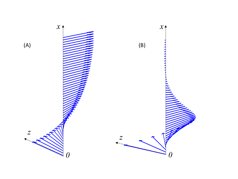
Figure 1: Schematic view of the spin rotation in a layered system with 1D inhomogeneity. At $x=0$ a spin parallel to the $z$-axis is injected. Due to the SO coupling also the $S^{y}$ component becomes finite upon diffusion. Panel (A) illustrates the spin rotation due to anisotropy of the Dyakonov-Perel tensor $\Gamma$. The vectors are given by Eqs.(12-13) and we have chosen $\beta/\alpha=1/3$. Panel (B) shows the spin rotation due to the second term in Eq. (11) for an isotropic SO coupling. The vectors are given in Eqs. (16-17) .

The second mechanism for spin rotation is the “precession” generated by the second term in the right hand side of Eq. (11). This mechanism is operative even for systems with equal relaxation rates for all spin directions. To illustrate the effect of this term we consider the simplest fully isotropic SO coupling described by the diagonal SO field ${\mathcal{A}}^{a}_{j}=\alpha\delta_{j}^{a}$. In this case Eq. (11) reduces to the following system of coupled diffusion equations for the spin components $S^{z}(x)$ and and $S^{y}(x)$

$$D\partial_{x}^{2}S^{z}+2D\alpha\partial_{x}S^{y}-\frac{S^{z}}{\tau_{s}} = 0,$$ (14)

$$D\partial_{x}^{2}S^{y}-2D\alpha\partial_{x}S^{z}-\frac{S^{y}}{\tau_{s}} = 0,$$ (15)

where $\tau_{s}=1/(2D\alpha^{2})$ is (now isotropic) spin relaxation time [in deriving this equations we made use of Eqs. (7) and (8)]. The coupling of different components of the spin in Eqs. (14)-(15) has a typical precession structure – it induces precession of the spin direction around the direction of inhomogeneity. Straightforward solution of these equations with the boundary condition ${\bf S}(x=0)=\hat{\bf z}S_{0}$ yields the helicoidal spin distribution,

$$S^{z}(x)=S^{z}_{0}e^{-\alpha x}\cos{\alpha x},$$ (16)

$$S^{y}(x)=S^{z}_{0}e^{-\alpha x}\sin{\alpha x},$$ (17)

which clearly demonstrates the effect of the precession term in the spin diffusion equation. The injected spin relaxes and rotates provided there is a spatial component of the SO field ${\mathcal{A}}_{k}^{a}$, or, more generally, the tensor $C_{k}^{ab}$, along the direction of inhomogeneity. In Fig. 1B we show schematically the spin rotation described by Eqs. (16-17).

In short, there are two mechanisms that can change the direction of the injected spin density. One originates from a possible anisotropy of the spin relaxation rate tensor $\Gamma^{ab}$ in Eq. (6), while the other mechanism is due to precession of the spin when $\hat{\rho}$ is spatially inhomogeneous according to the second term in the left hand side of Eq. (6). In the next section we show that these well established mechanisms for rotation of the spin also explain the rotation of the triplet component of the superconducting condensate and the appearance of a long-range proximity effect in SF hybrid structures with SO coupling.

III The singlet-triplet conversion in diffusive S/F structures: a physical picture

III.1 LRTC in S/F structures with SO coupling

We now discuss the singlet-triplet conversion in S/F structures in the presence of SO coupling. To pursue our line of reasoning we present in this section the linearized equation that describes the proximity effect in S/F structures and postpone its derivation to the next section.

We consider first the proximity effect in S/F structures without SO coupling. For simplicity we assume that the proximity effect is weak and therefore our starting point is the linearized Usadel equationUsadel which describes the superconducting condensate $\hat{f}$ induced in the diffusive ferromagnet F (see inset in Fig. 2)

$$D\nabla^{2}\hat{f}-2|\omega|\hat{f}-i{\mathrm{sgn}}(\omega)\{\hat{h},\hat{f}\}=0\;.$$ (18)

Here $\omega$ is the Matsubara frequency and $\hat{h}=h^{a}\sigma^{a}$ is the exchange field whose vector components $h^{a}$ may depend on space coordinates. This well-known equation, which has been used in most previous works on S/F structures (see for example Ref. BergeretRMP and references therein), describes diffusion of the condensate in the ferromagnet. The generation (injection) of the $s$-wave condensate at the S/F interface is commonly described by the Kupriyanov-Lukichev boundary condition KL which in its linearized version has a simple form

$$N_{k}{\partial}_{k}\hat{f}\big{|}_{S/F}=-\gamma f_{BCS},$$ (19)

where $f_{BCS}=\Delta/\sqrt{\omega^{2}+\Delta^{2}}$ is the anomalous Green’s function in the S-region, $N_{k}$ the $k$-component of the vector normal to the S/F interface, and $\gamma$ is a parameter that describes the quality of the S/F barrier. The boundary condition (19) works for interfaces with low transmission while for a perfect transparent barrier one should impose the continuity of $\hat{f}$ at the S/F interface.

Let us briefly recall the widely studied proximity effect in S/F structures without SO coupling. The most general form of the condensate function $\hat{f}$ satisfying Eqs. (18)-(19) is:Champel2005 ; Fominov2006

$$\hat{f}=f_{s}\hat{1}+f_{t}^{a}\sigma^{a}\;.$$ (20)

Here $f_{s}$ is the singlet component which is scalar in the spin space, while ${\bf f}_{t}$ is a vector in spin space (with components $f_{t}^{a}$) describing the triplet component. In the case of a spatially homogeneous exchange field ${\bf h}$ the condensate induced in F-region acquires both the singlet component $f_{s}$ and the triplet component ${\bf f}_{t}=f_{t}^{\parallel}{\bf h}/{h}$ with the spin along ${\bf h}$. Because of these two components the anticommutator in the right hand side of Eq. (18) is nonzero thus providing a coupling between the singlet $f_{s}$ and the parallel to ${\bf h}$ triplet $f^{\parallel}$ condensates. The magnitude of the coupling is given by the amplitude $h$ of the exchange field that is typically much larger than the characteristic energy ($\sim T$) of the second term in Eq. (18). Thus, the decaying length for both components away from the S/F interface is controlled by the singlet-triplet coupling, being of the order of $\xi_{h}=\sqrt{D/h}$. In other words, in the presence of a large exchange field the proximity effect becomes short ranged.

The structure of Eq. (18) suggests a way to circumvent the fast decay of superconducting correlations in ferromagnets. If by some means we generate components of the triplet condensate in any direction perpendicular to ${\bf h}$ the anticommutator in Eq. (18) vanishes and therefore those perpendicular components ${\bf f}_{t}^{\perp}$ will decay over the scale of the order of $\sqrt{D/T}$ which is much larger than $\xi_{h}$. It is very well established that such a long-range component, ${\bf f}_{t}^{\perp}$, can be induced in the presence of a spatially inhomogeneous vector ${\bf h}$Bergeret2001 ; BergeretRMP . But only recently it has been shown that SO coupling provides an alternative mechanism for generating the long-range triplet condensate.BT2013

Physically generation of the perpendicular component ${\bf f}_{t}^{\perp}$ can be viewed as a rotation of the triplet pair spin away from the direction of the exchange field.EschrigPT In the previous section we have seen that such a rotation is a generic feature of the spin diffusion in the presence of SO coupling and, as we now show, this feature should not depend on the nature of spin carriers, whether they are single electrons or triplet Cooper pairs.

In the presence of SO coupling the Usadel equation should be properly modified. As previously done, we consider only linear in momentum SO coupling describe by the Hamiltonian (3). In complete analogy with the spin diffusion in a normal system (see Section II) the SO-coupling-modified Usadel equation is obtained from Eq. (18) by replacing all derivatives with their covariant counterparts, $\partial_{k}\cdot\mapsto\tilde{\nabla}_{k}\cdot=\partial_{k}\cdot-i[\hat{{\mathcal{A}}}_{k},\cdot]$,

$$D\tilde{\nabla}^{2}\hat{f}-2|\omega|\hat{f}-i{\mathrm{sgn}}(\omega)\{\hat{h},\hat{f}\}=0\;.$$ (21)

To ensure that the condensate function $\hat{f}$ is transformed covariantly under a local SU(2) rotation the Kupriyanov-Lukichev boundary condition (19) should be also modified accordingly,

$$N_{k}\tilde{\nabla}_{k}\hat{f}\big{|}_{S/F}=-\gamma f_{BCS}.$$ (22)

The system of Eqs. (21), (22) describes the spatial distribution of the superconducting condensate induced from a s-wave superconductor in a ferromagnet with SO coupling. The covariant derivatives in these equations encode again all effects of SO coupling. If we now substitute the representation of Eq. (20) for the condensate function we obtain

$$D{\nabla}^{2}f_{s}-2|\omega|f_{s}-2i{\mathrm{sgn}}(\omega)h^{a}f_{t}^{a}=0\;,$$ (23)

$$D\nabla^{2}f_{t}^{a}+2C_{k}^{ab}\partial_{k}f_{t}^{b}-\Gamma^{ab}f_{t}^{b}-2|\omega|f_{t}^{a}-2i{\mathrm{sgn}}(\omega)h^{a}f_{s}=0\;,$$ (24)

from Eq. (21), and

$$N_{k}\partial_{k}f_{s}\big{|}_{S/F}=-\gamma f_{BCS}\;,$$ (25)

$$N_{k}(\partial_{k}f_{t}^{a}+C_{k}^{ab}f_{t}^{b})\big{|}_{S/F}=0\;,$$ (26)

from the boundary condition of Eq. (22). We have used the definitions of the Dyakonov-Perel spin relaxation tensor $\Gamma^{ab}$ and the diffusive spin precession tensor $C_{k}^{ab}$ presented in Eqs. (7) and (8). In the most general SO coupling, one can show, that the structure of Eqs. (23-26) remains the same with the tensors $\Gamma^{ab}$ and $C_{k}^{ab}$ redefined according to Eqs. (9) and (10).

The comparison of Eq. (24) with the spin diffusion equation (6) shows the complete analogy between spin diffusion in normal and superconducting systems. In particular, the physical effect of SO coupling is practically identical to that discussed in Sec. II.

By inspection of Eq. (24), it becomes clear that the direction of the condensate spin is not preserved in the F-region, due to the SO coupling. Similarly to the normal case the second and the third terms in Eq. (24) describe two mechanisms of the spin rotation – (i) a possible anisotropy of the relaxation rate, and (ii) the spin precession in the presence of a spatially inhomogeneous spin density. Therefore in the course of diffusion the spin of the condensate turns away from the direction of the exchange field. In other words a component perpendicular to ${\bf h}$ appears and decays over a length scale much larger than $\xi_{h}$. This slowly decaying part of ${\bf f}_{t}$ is responsible for the long-range proximity effect in S/F structures.

It is worth noting that the anisotropy of the spin relaxation rate generates the LRTC only if the direction of the exchange field does not coincide with one of the principal axes of the relaxation rate tensor $\hat{\Gamma}$. However, it is natural to expect that in realistic ferromagnets both ${\bf h}$ and the principal axes of $\Gamma^{ab}$ are linked to some crystallographic directions. Therefore it is quite probable that they do coincide and the mechanism (i) along is not sufficient to induce the LRTC in most of realistic situations. The second mechanism (ii), i.e. the spin precession mechanism is more likely to occur and more universal.

Because of its practical importance it is useful to have a simple illustrative example for the generation of LRTC via the spin precession mechanism. Let us consider the structure sketched in the inset of Fig.2. It is a S/F structure with the interface perpendicular to the $x$-axis (${\bf N}=\hat{\bf x}$) and the exchange field ${\bf h}=\hat{\bf z}h$ along $z$-axis. We assume a fully isotropic SO coupling with ${\mathcal{A}}_{k}^{a}=\alpha\delta_{k}^{a}$. By assuming that the structure has infinite dimensions in the z-y plane, the condensate function is invariant in this directions and only depends on x. Moreover, by symmetry, the triplet condensate function ${\bf f}_{t}$ has two components in spin space which lay in the z-y plane

$${\bf f}_{t}=f_{t}^{\parallel}\hat{\bf z}+f_{t}^{\perp}\hat{\bf y}\;.$$ (27)

Now the system of Eqs. (23)-(24) reads

$$D\partial_{x}^{2}f_{s}-2{|\omega|}f_{s}-2i{\mathrm{sgn}}(\omega){h}f_{t}^{\parallel}=0\;,$$ (30)

$$D\partial_{x}^{2}f_{t}^{\parallel}+2D\alpha\partial_{x}f_{t}^{\perp}-2\left(D\alpha^{2}+{|\omega|}\right)f_{t}^{\parallel}-2i{\mathrm{sgn}}(\omega){h}f_{s}=0\;,$$

$$D\partial_{x}^{2}f_{t}^{\perp}-2D\alpha\partial_{x}f_{t}^{\parallel}-2\left(D\alpha^{2}+{|\omega|}\right)f_{t}^{\perp}=0\;.$$

Equations (30-30) describe diffusion of strongly coupled singlet and parallel triplet condensates. The last, singlet-triplet coupling, terms $\sim h$ in these equations dominate, and, as a result, both $f_{s}$ and $f_{t}^{\parallel}$ decay over the short length scale $\sim\xi_{h}$. Equation (30) determines the spatial distribution of the perpendicular to ${\bf h}$ component $f_{t}^{\perp}$ of the triplet condensate. This component is generated near the interface because of the spin precession described by the second term and, according to Eq. (30), decays over a much longer length scale . The spatial distribution of all components of the condensate is shown in Fig. 2.

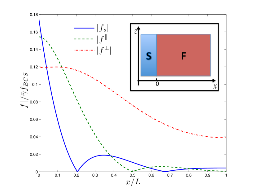
Figure 2: The spatial dependence of the amplitude of all components of the condensate function for the geometry shown in the inset and obtained from Eqs. (30-30) . The exchange field in F is homogeneous and points in $z$ direction. A fully isotropic SO coupling is assumed in F. We have chosen $h=10\Delta$, $\omega=\pi T$, $T=0.1\Delta$, $\alpha\xi_{0}=1$ and $L=1.5\xi_{0}$. Here $\Delta$ is the superconducting gap in S and the length $\xi_{0}$ is defined as $\xi_{0}=\sqrt{D/\Delta}$.

For a general SO field $\hat{\mathcal{A}}_{k}$ the LRTC is always induced if $\hat{\mathcal{A}}_{k}$ does not commute with the exchange field $\hat{h}$ and has a spatial component along the spin inhomogeneity. The condition $[\hat{h},\hat{\mathcal{A}}_{k}]\neq 0$ has an interesting interpretation in terms of SU(2) field tensor.BT2013 The exchange field enters the general many-body Hamiltonian as the time component of the SU(2) four-potential, $\hat{h}=\hat{\mathcal{A}}_{0}=\frac{1}{2}{\mathcal{A}}_{0}^{a}\hat{\sigma}^{a}$.Frolich93 ; Jin2006 ; Tokatly2008 ; Gorini2010 For the spatially uniform SU(2) potentials the above commutator is nothing but the SU(2) electric field $\hat{\mathcal{F}}_{k0}=-i[\hat{\mathcal{A}}_{k},\hat{\mathcal{A}}_{0}]$. Therefore the SU(2) electric field serves as a physical source of the LRTC in S/F structures, as it has been noticed recently in Ref. BT2013 . We will return to this point in the next subsection.

At this stage it is important to emphasize the difference between the SO coupling studied here, originated from the band structure or geometrical constraints (such as hetero-interfaces), and the SO effect caused by randomly distributed impurities.Abrikosv_Gorkov1961 The latter case has been studied intensively in the context of S/F structures.Demler ; Buzdin ; BVE_SO The only effect of the random SO coupling due to impurities is a finite, but fully isotropic spin relaxation rate. The direction of spin is always preserved and therefore no LRTC can be induced in this case.

We next show the connection between the inhomogeneous exchange field and the SO coupling as sources of long-range triplet component.

III.2 LRTC in a Bloch-like domain wall: a gauge-equivalent interpretation

The first theoretical work on the singlet-triplet conversion considered the case of a ferromagnet with a Bloch domain wall at the interface with a superconductor.Bergeret2001 It was assumed that the exchange field ${\bf h}$ in the F layer of the inset of Fig. 2 follows the magnetization direction that lies in the $y-z$ plane and rotates with respect to the $x$-axis. Thus ${\hat{h}}$ in Eq. (18) has the form:

$$\hat{h}=h\left[\sin(Qx)\sigma^{y}+\cos(Qx)\sigma^{z}\right]\;,$$

where $Q$ is the wave-vector of the rotation. In order to solve the linearized Usadel equation it is convenient to introduce the following local SU(2) rotation, as done in Ref. Bergeret2001 ,

$$\hat{\tilde{f}}(x)=U(x)\hat{f}U^{-1}(x)\;,$$ (31)

where $U(x)=e^{-\frac{i}{2}Qx\hat{\sigma}^{x}}$. Substitution of this expression into Eq. (18) removes the coordinate dependence from $h$

$$D\partial_{x}^{2}\hat{\tilde{f}}+\frac{DQ^{2}}{2}\left(\hat{\sigma}^{x}\hat{\tilde{f}}\hat{\sigma}^{x}-\hat{\tilde{f}}\right)+iDQ\left[\hat{\sigma}^{x},\partial_{x}\hat{\tilde{f}}\right]-2|\omega|\hat{\tilde{f}}-i{\rm sgn}\omega\left\{h\hat{\sigma}^{z},\hat{\tilde{f}}\right\}=0\;.$$ (32)

One can easily verify that this equation can be compactly written as:

$$D\tilde{\nabla}_{x}^{2}\hat{\tilde{f}}-2|\omega|\hat{\tilde{f}}-i{\rm sgn}\omega\left\{h\hat{\sigma}^{z},\hat{\tilde{f}}\right\}=0\,,$$ (33)

where

$$\tilde{\nabla}_{x}\cdot=\partial_{x}\cdot+i\frac{Q}{2}\left[\hat{\sigma}^{x},\cdot\right]\;.$$ (34)

Equation (33) is identical to Eq. (21) for a homogeneous exchange field ${\bf h}=h\hat{\bf z}$ and a SO coupling described by a “pure gauge” SU(2) potential $\hat{\mathcal{A}}_{x}=-(Q/2)\hat{\sigma}^{x}$ and $\hat{\mathcal{A}}_{y}=\hat{\mathcal{A}}_{z}=0$. This a remarkable result that demonstrates that the problem of the singlet-triplet conversion in a S/F structure with a Bloch domain wall is gauge-equivalent to the one of a ferromagnet with an homogeneous exchange field and a SO coupling. If we now compare Eq. (32) with Eqs. (23-24) in the context of the discussions in sections II and III.1, the second term in the l.h.s of Eq. (32) describes the Dyakonov-Perel relaxation with anisotropy typical for a pure gauge SO coupling Tokatly_Ann , while the third term induces the precession of the triplet component of the condensate and leads to the LRTC and the long-range proximity effect.

This example clearly shows the close connection between inhomogeneous exchange field and SO coupling by the generation of the LRTC. The inhomogeneous exchange field (inhomogeneous time component of the SU(2) potential $\hat{\mathcal{A}}_{0}$ ) at zero SO coupling $\hat{\mathcal{A}}_{k}=0$, and the homogeneous $\hat{\mathcal{A}}_{0}$ at nonzero $\hat{\mathcal{A}}_{x}$ describe the same physics in different gauges. The SU(2) electric field $\hat{\mathcal{F}}_{k0}=\partial_{k}\hat{\mathcal{A}}_{0}-i[\hat{\mathcal{A}}_{k},\hat{\mathcal{A}}_{0}]$, which is the source of the LRTC, is present in both cases, as it is a gauge covariant object. However, in one gauge $\hat{\mathcal{F}}_{k0}\neq 0$ because of inhomogeneity of $\hat{\mathcal{A}}_{0}$, while in the other gauge due to nonvanishing commutator $[\hat{\mathcal{A}}_{k},\hat{\mathcal{A}}_{0}]\neq 0$.

Before analyzing different S/F structures in the light of the SO coupling we present in the next section a more rigorous derivation of the main equation (21). Those readers not interested in technical details can skip next section and go directly to section V where we discuss the creation of long-range triplet correlations in different experimental setups.

IV Quasiclassical equations for systems with superconducting correlations, exchange field and spin-orbit coupling

The results of the previous section are based on Eq. (21) which has been obtained by simple gauge invariance arguments. In this section we present a formal derivation of the equations of motion for quasiclassical Green’s functions (GFs). We do not restrict our derivation to the equilibrium case and introduce the 8$\times$8 Keldysh GFs matrix

$$\mathbbm{G}({\bf r}_{1},{\bf r}_{2};t,t^{\prime})=\left(\begin{array}[]{cc}\check{G}^{R}&\check{G}^{K}\\ 0&\check{G}^{A}\end{array}\right)$$ (35)

where the retarded $\check{G}^{R}$, advanced $\check{G}^{A}$, and Keldysh $\check{G}^{K}$ GFs are 4$\times$4 matrices in the Nambu-Spin space. In principle we follow the standard derivation of the quasiclassical equation,LObook ; BergeretRMP but add the SO coupling described by the Hamiltonian (3). That is, we assume that SO coupling is linear in momentum, and the exchange field, $\hat{h}=h^{a}\sigma^{a}\equiv\hat{\mathcal{A}}_{0}$, does not depend on the momentum. In such a case the matrix (35) obeys the Dyson equation

$$\left[i\tau_{3}\partial_{t}+\check{G}_{0}^{-1}+\check{\Delta}-{\mathbb{\Sigma}}\right]\mathbbm{G}=1$$ (36)

where $\tau_{3}$ is the third Pauli matrix in Nambu space,

$$\check{G}_{0}^{-1}=\tau_{3}\hat{h}-\frac{1}{2m}\left(i\partial_{k}+\hat{{\mathcal{A}}}_{k}\right)^{2}+\mu\;,$$

$$\check{\Delta}=\left(\begin{array}[]{cc}0&\Delta\\ -\Delta^{*}&0\end{array}\right)\;,$$

$\mu$ is the chemical potential, $\Delta$ is the BCS order parameter and $\mathbb{\Sigma}$ is the self-energy describing the elastic scattering at non-magnetic impurities. In the Born approximation the self-energy reads ${\mathbb{\Sigma}}=(-i/2\tau)\langle{\mathbbm{g}}\rangle$. Here $\tau$ is the elastic scattering time, ${\mathbbm{g}}$ is the GF matrix integrated over quasiparticle energy and $\langle\dots\rangle$ stands for the average over the Fermi momentum direction.

To simplify the derivation of the quasiclassical equations we assume for a moment that the exchange field $\hat{h}$ and the SO field $\hat{\mathcal{A}}_{k}$ do not depend on spatial coordinates. We will see that the full space dependence can be recovered at the end in the final equations from symmetry arguments.

By following the standard routeLObook we first subtract from Eq. (36) its conjugate, and go to the Wigner representation in space by performing the Fourier transformation with respect to the coordinate difference $\bm{\xi}={\bf r}_{1}-{\bf r}_{2}$. Then we proceed to the gradient expansion up to first order in derivatives with respect to the “center of mass” coordinate ${\bf r}=\frac{{\bf r}_{1}+{\bf r}_{2}}{2}$. This procedure leads to the following equation for the Wigner transformed matrix $\mathbbm{G}({\bf p},{\bf r};t,t^{\prime})$

$$\tau_{3}\partial_{t}{\mathbbm{G}}+\partial_{t^{\prime}}{\mathbbm{G}}\tau_{3}-i\left[\tau_{3}\hat{h},{\mathbbm{G}}\right]+\frac{1}{2m}\left\{p_{k}-\hat{{\mathcal{A}}}_{k},\partial_{k}{\mathbbm{G}}\right\}-i\frac{p_{k}}{m}\left[\hat{{\mathcal{A}}}_{k},{\mathbbm{G}}\right]-i\left[\check{\Delta},{\mathbbm{G}}\right]=-\frac{1}{2\tau}\left[\langle\mathbbm{g}\rangle,{\mathbbm{G}}\right]\;.$$ (37)

It is instructive to estimate the order of magnitude of different terms in this equation. Let $T$ and $L$ be characteristic time and length scales, that is, $\partial_{t}\sim 1/T$ and $\partial_{{\bf r}}\sim 1/L$. Since $\mathbbm{G}$ as a function of ${\bf p}$ is peaked at $p_{F}$, all momenta in Eq. (37) are of the order of $p_{F}$. Within the validity of semiclassical approach we assume that energies corresponding to $T^{-1}$, $v_{F}/L$, the momentum relaxation rate $\tau^{-1}$, the exchange energy $h$, SO spin splitting $v_{F}{\mathcal{A}}$, and the superconducting gap $\Delta$ are allowed to be of the same order of magnitude, but should all be much smaller than the Fermi energy $\varepsilon_{F}$. The ratio $\eta=\varepsilon_{\rm dyn}/\varepsilon_{F}$ of the above small dynamical energy scales to $\varepsilon_{F}$ is the small parameter that justifies the quasiclassical approximation in quantum kinetics.

Now we can look on Eq. (37) from this point of view. Apparently all, except one, terms in Eq. (37) can be of the same order of magnitude being linear in the small parameter $\eta$. Only one term $\sim\hat{{\mathcal{A}}}_{k}\partial_{k}{\mathbbm{G}}$ in the left hand side has and extra factor of the order of ${\mathcal{A}}/p_{F}\sim\eta$. In the leading order of the semiclassical expansion it is absolutely natural to neglect this term. However it is also important to understand what are the physical consequences of this term and which effects we drop out by neglecting it.

The physics of the subleading term can be revealed by transforming the kinetic equation Eq. (37) to the gauge covariant form in which SU(2) field strengths and the corresponding forces appear explicitly. For this sake we use the technique of gauge covariant Wigner functions, which has been developed originally in the context of quark-gluon kinetic theoryHeinz and applied more recently to describe the spin dynamics in semiconductors.Gorini2010 The main idea of this approach is to switch from the usual GF of Eq. (35) to its “gauge covariant” counterpart that is defined as follows

$$\tilde{\mathbbm{G}}({\bf r}_{1},{\bf r}_{2};t,t^{\prime})=\hat{W}({\bf r},{\bf r}_{1}){\mathbbm{G}}({\bf r}_{1},{\bf r}_{2},t,t^{\prime})\hat{W}({\bf r}_{2},{\bf r})\;,$$ (38)

where $\hat{W}({\bf r},{\bf r}_{1})$ and $\hat{W}({\bf r}_{2},{\bf r})$ are the Wilson link operators which “covariantly connect” the arguments of the Green’s function to the ”center-of-mass” coordinate ${\bf r}=\frac{{\bf r}_{1}+{\bf r}_{2}}{2}$. Formally the Wilson link operator entering this equation is defined by the path-ordered exponential $\hat{W}({\bf r}_{2},{\bf r}_{1})=P\exp{[i\int_{C_{12}}\hat{{\mathcal{A}}}_{j}dx_{j}]}$, where the integration path $C_{12}$ goes from ${\bf r}_{1}$ to ${\bf r}_{2}$ along the straight line. Heinz The advantage of the GF $\tilde{\mathbbm{G}}$ in Eq. (38) over the usual GF $\mathbbm{G}$ is that the Wigner transform of $\tilde{\mathbbm{G}}$, and thus the corresponding quasiclassical GF $\tilde{\mathbbm{g}}({\bf r})$, will transform locally covariantly under a nonuniform SU(2) rotation $\hat{U}({\bf r})$, i. e. $\tilde{\mathbbm{g}}({\bf r})\mapsto\hat{U}({\bf r}){\tilde{\mathbbm{g}}}({\bf r})\hat{U}^{-1}({\bf r})$.

In our case of spatially homogeneous SU(2) potentials $\hat{{\mathcal{A}}}_{k}$ the Wilson link operators reduce to a simple matrix exponential

$$\hat{W}({\bf r},{\bf r}_{1})=\hat{W}({\bf r}_{2},{\bf r})=e^{\frac{i}{2}\hat{{\mathcal{A}}}_{k}(r_{1}^{k}-r_{2}^{k})}.$$

Obviously, in this case the Wigner transformation of Eq. (38) can be performed explicitly. The result is the following relation between the Wigner transforms of the usual $\mathbbm{G}$ and the covariant one $\tilde{\mathbbm{G}}$

$${\mathbbm{G}}({\bf r},{\bf p};t,t^{\prime})=e^{-\frac{1}{2}{\hat{\mathcal{A}}}_{k}\overrightarrow{\partial_{p_{k}}}}\tilde{\mathbbm{G}}({\bf r},{\bf p};t,t^{\prime})e^{-\frac{1}{2}{\hat{\mathcal{A}}}_{k}\overleftarrow{\partial_{p_{k}}}},$$ (39)

where the upper arrow in the operators $\overrightarrow{\partial_{p_{k}}}$ and $\overleftarrow{\partial_{p_{k}}}$ indicate the direction in which the momentum derivative is acting.

Now we can derive the equation for $\tilde{\mathbbm{G}}$ by substituting Eq. (39) into Eq. (37) and then acting from the left with $\exp\{-\frac{1}{2}{\hat{\mathcal{A}}}_{k}\overrightarrow{\partial_{p_{k}}}\}$, and from the right with $\exp\{-\frac{1}{2}{\hat{\mathcal{A}}}_{k}\overrightarrow{\partial_{p_{k}}}\}$. Finally, by making an expansion up to first order in the gradients and second order in SO fields $\hat{{\mathcal{A}}}_{k}$, we obtain the following equation for the gauge covariant function $\tilde{\mathbbm{G}}$

$$\tau_{3}\partial_{t}\tilde{\mathbbm{G}}+\partial_{t^{\prime}}\tilde{\mathbbm{G}}\tau_{3}-i\left[\tau_{3}\hat{h},\tilde{\mathbbm{G}}\right]+\frac{p_{k}}{m}\tilde{\nabla}_{k}\tilde{\mathbbm{G}}+\frac{1}{2\tau}\left[\langle\tilde{\mathbbm{g}}\rangle,\tilde{\mathbbm{G}}\right]-i\left[\check{\Delta},\tilde{\mathbbm{G}}\right]=\frac{1}{2}\left\{\tau_{3}\hat{\mathcal{F}}_{0k}+\frac{p_{k}}{m}\hat{\mathcal{F}}_{kj},\partial_{p_{j}}\tilde{\mathbbm{G}}\right\}\;,$$ (40)

where $\tilde{\nabla}_{k}\cdot=\partial_{k}\cdot-i[\hat{\mathcal{A}}_{k},\cdot]$ is the covariant gradient. In the right hand side of this equation we introduced the SU(2) field strength tensors $\hat{\mathcal{F}}_{0k}=-i[\hat{h},\hat{\mathcal{A}}_{k}]$ and $\hat{\mathcal{F}}_{kj}=-i[\hat{\mathcal{A}}_{k},\hat{\mathcal{A}}_{j}]$.

Formally Eq. (40) was derived for spatially homogeneous exchange $\hat{h}$ and SO ${\mathcal{A}}_{k}$ fields. It is, however, absolutely clear that all we need to account for possible (static) inhomogeneities of the spin-dependent fields is to use for the SU(2) electric $\hat{\mathcal{F}}_{0k}$ and $\hat{\mathcal{F}}_{kj}$ the full expressions

$$\hat{\mathcal{F}}_{0k} = -\partial_{k}\hat{h}-i[\hat{h},\hat{\mathcal{A}}_{k}],$$ (41)

$$\hat{\mathcal{F}}_{kj} = \partial_{k}\hat{\mathcal{A}}_{j}-\partial_{j}\hat{\mathcal{A}}_{k}-i[\hat{\mathcal{A}}_{k},\hat{\mathcal{A}}_{j}].$$ (42)

An advantage of Eq. (40) over the original and more common Eq. (37) is the explicit SU(2) gauge covariance of the former. The SO coupling enters Eq. (40) only via the covariant gradient $\tilde{\nabla}_{k}$ and the SU(2) field tensor $\hat{\mathcal{F}}_{\mu\nu}$. Now the physical significance of the subleading contribution to the kinetic equation can be easily identified. The subleading terms, of the order of $\eta^{2}$, are collected on the right hand side of Eq. (40). These terms describe the SU(2) Lorentz force Gorini2010 which, in particular, is responsible for the coupling of spin and charge degrees of freedom and the spin Hall effect. The leading contribution of SO coupling is exhausted by the covariant gradient term in the left hand side of Eq. (40). Physically it describes spin precession in the presence of the effective momentum dependent SO Zeeman field.

In the present paper we consider only the leading (spin precession) effects of SO coupling, while the terms of higher order in $\eta$ (the SU(2) Lorentz force effects) will be neglected. Obviously the latter have to be taken into account to study phenomena involving spin-charge coupling due to SO coupling.Stanescu2007 ; Gorini2010 It is worth noting that Eqs. (37) and (40) become identical if we neglect terms of the order $\eta^{2}$.

After neglecting the right hand side in Eq. (40) one can easily integrate this equation over the quasiparticle energy and, by using the fact that the ${\tilde{\mathbbm{G}}}$ is peaked at the Fermi level, one obtains the SU(2) covariant Eilenberger equation

$$\tau_{3}\partial_{t}{\mathbbm{g}}+\partial_{t^{\prime}}{\mathbbm{g}}\tau_{3}-i\left[\tau_{3}\hat{h},{\mathbbm{g}}\right]+v_{F}n_{k}\tilde{\nabla}_{k}{\mathbbm{g}}-i\left[\check{\Delta},{\mathbbm{g}}\right]=-\frac{1}{2\tau}\left[\langle{\mathbbm{g}}\rangle,{\mathbbm{g}}\right]\;,$$ (43)

where ${\mathbbm{g}}({\bf n},{\bf r},t,t^{\prime})$ is the quasiclassical GFs that depends on the Fermi momentum direction ${\bf n}={\bf p}_{F}/p_{F}$, the center of mass coordinate ${\bf r}$ and two times. In the diffusive case this equation can be further simplified by assuming that the GFs have a weak dependence on the momentum direction, i. e. by approximating ${\mathbbm{g}}\approx{\mathbbm{g}_{0}}+{{\bf n}}{\mathbbm{g}_{1}}$. Following the standard derivation for diffusive equations (see for example LObook ) one finally arrives at the Usadel equation for the isotropic part ${\mathbbm{g}_{0}}$ (we skip the index $0$):

$$D\tilde{\nabla}_{k}({\mathbbm{g}}\tilde{\nabla}_{k}{\mathbbm{g}})+\tau_{3}\partial_{t}{\mathbbm{g}}+\partial_{t^{\prime}}{\mathbbm{g}}\tau_{3}-i\left[\tau_{3}\hat{h},{\mathbbm{g}}\right]-i\left[\check{\Delta},{\mathbbm{g}}\right]=0,$$ (44)

where $D=v_{F}^{2}\tau/3$ is the diffusion coefficient. We note that in the absence of superconducting correlations this equation leads to the spin diffusion equation (4) or, equivalently, Eq. (6).

Throughout this article we only analyze equilibrium situations. In this case it is convenient to work with the Matsubara GF $\check{g}({\bf r},\omega)$ which is a $4\times 4$ matrix in the Nambu-spin space. The corresponding Usadel equation can be obtained straightforwardly from Eq. 44 (see for example BergeretRMP ):

$$D\tilde{\nabla}_{k}(\check{g}\tilde{\nabla}_{k}\check{g})+\omega[\tau_{3},\check{g}]-i\left[\tau_{3}\hat{h},\check{g}\right]-i\left[\check{\Delta},\check{g}\right]=0\;,$$ (45)

where $\omega$ is the Matsubara frequency. Moreover, we only focus on the linearized Usadel equation which is valid either at temperatures close to the critical temperature or in the non-superconducting regions if the proximity effect is weak enough. In such a case one can expand the GF’s functions according to $\check{g}\approx\tau_{3}{\rm sgn}(\omega)+i\tau_{2}{\hat{f}}$ where ${\hat{f}}$ is the anomalous Green function describing the superconducting condensate. We finally obtain

$$D\tilde{\nabla}^{2}\hat{f}-2|\omega|\hat{f}-i{\mathrm{sgn}}(\omega)\left\{\hat{h},\hat{f}\right\}=0\;,$$ (46)

which coincides with Eq. (21) used along the manuscript.

V Examples of singlet-triplet conversion in hybrid structures with SO coupling

Figure 3: Different geometries discussed in the main text. (A) A S/F/N_SO structure. It is assumed that a finite Rashba SO coupling is present in the normal wire N_SO . (B) A lateral S/F structure consisting of a thin ferromagnetic layer F₁, a superconductor electrode and a second ferromagnetic layer, F₂ between the S and the F₁. The S/F₂ structure extends over the $x<0$ region. (C) Sketched of a transversal multilayer structure commonly used in experiments and (D) its analog analyzed in the text.

V.1 S/F/N structure with SO coupling

As we have seen in sections II and III.1, the SO coupling causes both the spin rotation in normal metals and the ”rotation” of the triplet component of the condensate in S/F structures. From this analogy one can infer that if a triplet component is induced in a diffusive normal metal with SO coupling, such component may rotate leading to components perpendicular to the original one. One can corroborate this statement by the following example, that represents a novel way of generation of the LRTC.

We consider a S/F/N_SO lateral structure as the one shown in Fig. 3A: A S/F bilayer is situated on top of a thin and narrow normal region, like a normal wire.jain0 The S/F bilayer extends to the left ($x<0$) and the normal wire has some intrinsic SO coupling. The F layer is sufficiently thin in order to allow for superconducting correlations to penetrate into the N wire. Notice that this geometry, without the F layer, resembles pretty much the setup proposed for detection of Majorana fermions in hybrid structures. DasSarma ; Majorana_exp

To simplify formalities we assume that the S/F interface is transparent and both layers are thin enough to describe them as an effective ferromagnetic superconductorBergeret2001b ; Giazotto2013 with effective values for the order parameter $\Delta_{eff}=\Delta\nu_{S}d_{S}/(\nu_{S}d_{S}+\nu_{F}d_{F})$ and the exchange field $h_{eff}=h\nu_{F}d_{F}/(\nu_{S}d_{S}+\nu_{F}d_{F})$, where $d_{S(F)}$ is the thickness of the S(F) layer and $\nu_{S(F)}$ its density of the states. Thus, the SF layer exhibits a BCS-like density of states which is now spin-dependent shifted by $h_{eff}$. If the exchange field lies in the $(x,y)$ plane (see Fig. 3A) the condensate function in the S/F electrode consists, as usual, of a singlet $f_{FS}^{s}=f_{+}$ and a triplet component that reads

$$\hat{f}_{SF}^{t}=f_{-}(\cos\theta\sigma^{x}+\sin\theta\sigma^{y})\;,$$ (47)

where $f_{\pm}=[f_{BCS}(\omega+ih_{eff})\pm f_{BCS}(\omega-ih_{eff})]/2$, and $\theta$ is the angle between the exchange field and the $x$-axis. In this way, the function of the S/F electrode is to generate in the normal metal the triplet component parallel to the exchange field of F. In analogy to the spin diffusion in a normal metal (cf. Section II), the induced triplet component is eventually rotated in the N_SO wire and all other triplet components generated as we discuss next.

If the N_SO wire is deposited on a substrate it is natural to assume that the SO coupling is described by ${\mathcal{A}}_{x}^{y}=\alpha$, while all other components of $\hat{\mathcal{A}}$ are zero. Moreover, we assume that the width $d$ of the normal wire is much smaller than the characteristic variation of condensate induced via proximity effect. Thus, we can integrate the Usadel Eq. (21) over the z-direction by using the boundary condition Eq. (22) which now reads:

$$\partial_{z}f_{s} = -\gamma f_{+}^{s}$$ (48)

$$\partial_{z}f_{t}^{a}\sigma^{a} = -\gamma f_{-}\left(\cos\theta\delta^{ax}+\sin\theta\delta^{ay}\right)\;.$$ (49)

With all these assumptions and after integration over $z$-direction we end up with the following set of 1D linear differential equations:

$$\partial^{2}_{x}f_{s}-\kappa_{\omega}^{2}f_{s} = \frac{\gamma}{d}f_{+}\Theta(-x)$$ (50)

$$\partial^{2}_{x}f_{t}^{y}-\kappa_{\omega}^{2}f_{t}^{y} = \frac{\gamma}{d}f_{-}\sin\theta\Theta(-x)$$ (51)

$$\partial^{2}_{x}f_{t}^{x}-(\kappa_{\omega}^{2}+\alpha^{2})f_{t}^{x}+2\alpha\partial_{x}f_{t}^{z} = \frac{\gamma}{d}f_{-}\cos\theta\Theta(-x)$$ (52)

$$\partial^{2}_{x}f_{t}^{z}-(\kappa_{\omega}^{2}+\alpha^{2})f_{t}^{z}-2\alpha\partial_{x}f_{t}^{x} = 0\;,$$ (53)

where $\Theta(x)$ is the Heaviside step-function and $\kappa_{\omega}^{2}=2|\omega|$. It is straightforward to obtain the solution of this system. We present here only the solution for the triplet components of the condensate in the region $x>0$ (Fig. 3A):

$$\hat{f}_{t}={\cal C}_{\omega}f_{-}e^{-\kappa_{\omega}x}\left[\cos(\alpha x)\cos\theta\sigma^{x}+\sin\theta\sigma^{y}+\sin(\alpha x)\cos\theta\sigma^{z}\right]\;,$$ (54)

where ${\cal C}_{\omega}=-\gamma/[2d(\kappa_{\omega}^{2}+\alpha^{2})]$. As expected, the ”injected” triplet component of the condensate, which is parallel to the exchange field of the S/F bilayer, can rotate if a finite SO coupling exists in the normal region. For this to occur the SO coupling must satisfy $[\hat{\mathcal{A}}_{k},\hat{\mathcal{A}}_{0}]\neq 0$. In our particular case ($\hat{\mathcal{A}}_{x}=\frac{1}{2}\alpha\sigma^{y}$) the perpendicular components are generated provided that the exchange field is not pointing in the $y$-direction. In the latter case, as one can directly see from Eq. (54), only the parallel component is generated in N_SO. The presence of the SO coupling leads to a spatial oscillation of the $f^{x}_{t}$ and $f_{t}^{z}$ components as shown in Fig. 4. We should emphasize however, that this oscillation has another origin as the one discussed in the context of SF structures without spin-orbit.BuzdinRMP ; Ryazanov2001 In the latter case the oscillations in the F layer are due to the presence of a (homogenous) exchange field which also affects the singlet component. Here however, there is no exchange field in the N region and the oscillations are simple due to the SO term in analogy to the spin rotation in normal systems. Notice that in our geometry the singlet component does not oscillate and no 0-$\pi$ transition is expected in a symmetric S/F/N_SO/F/S Josephson junction, in contrast to the oscillations in the critical current observed in SFS structures.Ryazanov2001

In principle the S/F/N_SO structure described here can be used as a generator of the LRTC . If we assume, for example that at the other end of the N_SO wire there is second strong ferromagnet with a magnetization parallel to the ”injector” F the component $f_{t}^{x}$ of the condensate will penetrate this second ferromagnet over long distances of the order of $\sqrt{D/T}$. We notice that the mechanism discussed in this section also explains the triplet component induced in a superconductor-2D normal metal-superconductor junction with Rashba SO coupling in an external Zeeman field discussed in Ref.Malshukov . It is also worth to mention that a similar (but in the ballistic limit) has been analyzed in a recent manuscript.jain0

Figure 4: The spatial behavior of the singlet and triplet components $f_{t}^{z}$ and $f_{t}^{x}$ in the normal region of the structure shown in Fig. 3A obtained from Eqs. (50)-(53). We have chosen $\omega=\pi T$, $\alpha\xi_{0}=1$ and $T=0.1\Delta_{0}$, and $\theta=0$. The values of $f_{s}$ and $f_{t}^{x}$ are normalized to their asymptotic values at $x=-\infty$, while $f_{t}^{z}$ is normalize to the asymptotic value of $f_{t}^{x}$.

V.2 Lateral Josephson junction with SO coupling

The first evidence of long-range superconducting correlations in magnetic materials was found by measuring a finite supercurrent flowing through a half-metallic CrO₂ in a lateral Josephson junction Keizer2006 (see sketch in Fig. 3B). The supercurrent across the junction could be observed up to distances of the order of one micron between the S leads and can only be explained by assuming that the supercurrent is carried by Cooper pairs with equal spin projection, or in our terminology by assuming a finite triplet component of the condensate perpendicular to the magnetization direction of the half-metal. The required spin-triplet conversion might take place in a region around the S/F interface if one assumes a magnetic disorder with a finite averaged moment misaligned with respect to the bulk magnetization of the CrO₂ layer.Eschrig2008 It is difficult to prove experimentally such inhomogeneity. More recent experiments on CrO₂ based Josephson junctions have shown that the observation of long-range effects depends on the substrate on which the half metal is grown. For example, generation of the long-range triplet component has been observed in CrO₂ grown onto Al₂O₃ by using simple superconducting contacts. In contrast, if the CrO₂ is grown onto a TiO₂ substrate, the long-range Josephson effect can only be observed if one incorporates a thin Ni layer between the CrO₂ and the superconducting electrodes. Aarts2010 ; Aarts2012 It is commonly believed that in both cases the long-range triplet component is generated due to a magnetic inhomogeneity, either originated at the superconductor/CrO₂ interface (spin-active interface) or in the Ni interlayer.Yates2013

We give here an additional possible explanation for the long-range proximity effect in such lateral structures, based on the presence of SO coupling at the contact region. The existence of a SO coupling in the CrO₂ experiments was suggested in Ref. Yates2013 , but not discussed quantitatively due to the lack of a formalism for this. We have now all ingredients to include the SO coupling in the study of the proximity effect, and focus our analysis on the system sketched in Fig. 3B . It is a lateral structure consisting of a superconductor S and a ferromagnet F₁. At the interface between them there is an additional thin layer, F₂, with a magnetization parallel to the F₁ layer. Thus, in principle, one does not expect any long-range effect in accordance with previous theories. BergeretRMP We assume that in F₂ there is a finite SO coupling , which can be either due to some crystallographic inversion asymmetrySamokhin2009 or due to the presence of interfaces between materials and the lack of structure inversion symmetry.Rashba ; Edelstein2003 ; Koroteev2004 ; Ast2007 ; Miron2010 ; Linder2011 ; Duckheim2011 ; Takei2012 ; Takei2013

The S/F₂ bilayer extend over the whole negative $x-axis$ and the SO coupling is only present in the F₂ layer and therefore the SO vector potential is written as:

$${\mathcal{A}}^{a}_{j}(z,x)={\mathcal{A}}^{a}_{j}\Theta(-x)\Theta(-z)\Theta(z+d)\;.$$ (55)

If one assumes translation invariance in $y$ direction then the condensate function in Eq. (21) depends on $x$ and $z$ coordinates (see Fig. 3B) and satisfies Eqs. (23-24). This problem can be solved numerically. However, in order to underline the physics of the singlet-triplet conversion we solve here the problem analytically by assuming first that the total thickness $W+d$ is much smaller than the characteristic length over which the condensate $f$ changes. This assumption allows us to integrate the Usadel equation over $z$. Secondly, we neglect quadratic terms in ${\mathcal{A}}$, by assuming that $|{\mathcal{A}}|^{2}\ll h/D$. This means we neglect the term proportional to $\Gamma$ in Eq. (24). After integration over the $z$-direction and by using the boundary condition Eq. (22) at the S/F₂ and continuity at F₁/F₂ interfaces we obtain from Eqs. (23-24)

$$D\partial^{2}_{xx}fs-2|\omega|f_{s}-2i{\rm sgn}(\omega)h^{x}f^{x}_{t} = -\frac{D\gamma}{W+d}f_{BCS}\;,$$ (56)

$$D\partial^{2}_{xx}f_{t}^{a}-2|\omega|f_{t}^{a}-2i{\rm sgn}(\omega)h^{x}f_{s}+\frac{2d}{d+W}{C}^{ab}_{x}\partial_{x}f_{t}^{b} = 0\;,$$ (57)

for $x<0$, and

$$D\partial^{2}_{xx}f_{s}-2|\omega|f_{s}-i{\rm sgn}(\omega)h^{x}_{1}f^{x}_{t} = 0\;,$$ (58)

$$D\partial^{2}_{xx}f_{t}^{a}-2|\omega|f_{t}^{a}-i{\rm sgn}(\omega)h^{x}_{1}f_{s} = 0\;,$$ (59)

for $x>0$. Here $h_{1,2}$ are the exchange fields (that point in $x$-direction) in the F_1,2 regions and $h=h_{1}W/(W+d)+h_{2}d/(W+d)$ is the averaged exchange field. We assume that the SO coupling is of Rashba type with $C_{x}^{xz}=-D\alpha$. These equations have to be solved assuming that the condensate function is continuous at $x=0$ and

$$\left.\partial_{x}\hat{f}+i\frac{d}{d+W}\alpha\left[\sigma^{y},\hat{f}\right]\right|_{x=0^{-}}=\left.\partial_{x}\hat{f}\right|_{x=0^{+}}\;.$$ (60)

From a simple inspection of Eqs. (56-60) one can conclude that a finite triplet component, $f_{t}^{x}$ perpendicular to the exchange field is generated by the SO coupling term. The decay of this component into the $x>0$ is long-range as follows from Eq. (59). Deep in the region covered by the S/F₂ bilayer ($x\rightarrow-\infty$) the solution does not depend on $x$ and according to Eq. (56) is given by

$$f_{s}(-\infty) \approx \frac{\gamma\xi_{h}^{2}}{W+d}\frac{|\omega|}{2h}f_{BCS}$$ (61)

$$f_{t}^{x}(-\infty) \approx -i\frac{\gamma{\rm sgn}(\omega)\xi_{h}^{2}}{2(W+d)}f_{BCS}$$ (62)

$$f_{t}^{z}(-\infty) = 0;\,$$ (63)

where $\xi_{h}=\sqrt{D/h}$ (we have assumed that $h_{1}\gg h_{2},T$). Notice that the asymptotic value of the ”perpendicular” component of the triplet $f_{t}^{z}$, is zero. In principle one can obtain straightforwardly the spatial dependence for all condense components by solving the boundary problem Eqs. (56-60). Here we present the solution for the long-range component $f_{t}^{z}$ in the region $x>0$. It is given by

$$f_{t}^{z}(x>0)=\frac{3}{2}i{\rm sgn}(\omega)\frac{\alpha d\xi_{\omega}\xi_{h}^{2}}{(W+d)^{2}}f_{BCS}e^{-\kappa_{\omega}x}$$ (64)

where $\kappa_{\omega}^{-1}=\sqrt{D/2|\omega|}$ is the characteristic decay-length. If we now assume that at $x=L\gg\xi_{h}$ there is a second S/F₂ electrode one can easily shown the (spectral) Josephson current through the junction decays as BT2013 $e^{-\kappa_{\omega}L}$ with the junction length $L$. This confirms the long-range character of the proximity effect. It is important to emphasize that the magnetization of all F layers has been assumed to be parallel. The long-range component, Eq. (64), is proportional to the SO coupling $\alpha$ in the F₂ thin layer. This example clearly shows that besides magnetic inhomogeneity, the SO coupling can also be a source for the LRTC.

V.3 Multilayer transversal structures

Apart of the experiments on CrO₂ lateral structures, most of the experiments searching for triplet long-range proximity effect have been performed on transversal structuresBirge2010 ; Robinson2010 ; Sprungmann2010 ; Usman2011 ; Birge2012 as the one sketched in Fig. 3C. The region between the S electrodes consists of a multilayered magnetic structure that provides the magnetic inhomegeneity for the singlet-triplet conversion. Again, due to the hetero-interfaces between different materials one can expect a finite SO coupling in the structure.Edelstein2003 ; Linder2011 In order to simplify the problem, instead of analyzing the multilayer system of Fig. 3C, we study here the SF_SOS junction of Fig. 3D, by assuming that the F_SO, besides the in-plane exchange field, exhibits also a SO coupling of the form:

$$\hat{\mathcal{A}}_{z} = \beta\sigma^{z}-\alpha\sigma^{y}\;,$$ (65)

$$\hat{\mathcal{A}}_{y} = -\beta\sigma^{y}+\alpha\sigma^{z}\;,$$ (66)

where $\alpha$ and $\beta$ are known in the literature as the Rashba and Dresselhaus constants respectively. The system is translation invariant in the $(x,y)$ plane and therefore it is unlikely to have a finite component of the vector potential $\hat{\mathcal{A}}_{k}$ in $z$ direction. Moreover the condensate function $\hat{f}$ only varies over $x$ direction and therefore the second term in Eq. (24) does not contribute. This means that, eventually, the only source for the LRTC is the relaxation rate tensor $\Gamma^{ab}$, defined in Eqs. (6-8). Thus, the condition for generating the long triplet component, i. e. the component perpendicular to the exchange field is that the vector $\left[\hat{\mathcal{A}}_{k},\left[\hat{\mathcal{A}}_{k},h^{a}\sigma^{a}\right]\right]$ is not parallel to the exchange field $h^{a}\sigma^{a}$. For the SO coupling described by Eqs. (65-66) one obtains

$$\left[\hat{\mathcal{A}}_{k},\left[\hat{\mathcal{A}}_{k},h^{a}\sigma^{a}\right]\right]=4(\alpha^{2}+\beta^{2})(h^{a}\sigma^{a}+h^{x}\sigma^{x})+8\alpha\beta(h^{y}\sigma^{z}+h^{z}\sigma^{y})\;.$$ (67)

If the magnetization points in the perpendicular direction (i. e. $h^{y}=h^{z}=0$) then the LRTC is not generated. If all components of the exchange field are finite (as in the case of Ho layers Robinson2010 ) the term proportional to $\Gamma^{ab}$ in Eq. (24) generates LRTCs for any value of $\alpha$ and $\beta$.

In the most common case of an in-plane magnetization $h^{x}=0$, the condition for the LRTC is that $\alpha\beta\neq 0$ and $h^{y}\neq h^{z}$. It is important to emphasize that this condition for triplet generation is more restrictive than in the lateral geometry studied in previous section, in which a pure Rashba SO coupling at the S/F interface and arbitrary magnetization orientation are enough for the LRTC to exist.

VI Conclusions

The SO coupling discussed here has its origin in the lack of inversion symmetry and therefore it has to be distinguished from the SO coupling originated by disorder which does not generate the long-range triplet component and it was widely studied in the past decades. On the one hand the lack of inversion symmetry can be due to some crystallographic inversion asymmetry in the materials. However, such noncentrosymmetric metals have not been experimentally explored in the context of superconducting proximity effect. A detailed analysis of these materials based on the symmetry arguments can be found in the review Ref. Samokhin2009 . On the other hand, the lack of inversion symmetry can also occur at the interface between two different materials inducing an interfacial SO coupling.Edelstein2003 ; Koroteev2004 ; Ast2007 ; Miron2010 ; Linder2011 ; Duckheim2011 ; Takei2012 ; Takei2013 This might be the scenario in some of the structures used in the experiments on SFS junctions. It is not straightforward to estimate the strength of the SO coupling for a given hybrid interface. This has been obtained from first principle calculations for certain material combinations.Ast2007 Also experiments exploring spin torque in Pt/Co/AlO_x multilayer, provide a pretty large value for the SO coupling induced by the inversion asymmetry of the structure.Miron2010 A considerable SO coupling is also predicted for other metallic interfaces.Manchon2008

In conclusion, we have presented an exhaustive study of the proximity effect in diffusive superconductor-ferromagnet hybrid structures with spin-orbit coupling. We have derived the quasiclassical equations that include generic spin fields. For the particular case of spin-orbit coupling linear in momentum, we have drawn an useful and novel analogy between the spin precession in a normal diffusive system with SO coupling and the generation of the long-range triplet component in S/F structures. As for a spin density in a normal system , the presence of a SO coupling may rotate the triplet component of the superconducting condensate and generate all triplet projections. We explicitly demonstrate that both, the spin diffusion equation in the normal state and the linearized Usadel equation describing the proximity effect in SF structures with SO coupling, are almost identically. This analogy provides a useful tool for the design of experimental setups and the search of optimal material combinations for the control and manipulation of the triplet component in hybrid superconducting structures. Moreover, it suggests a possible way to control and manipulate the spin in low dissipative devices based on S/F hybrids with spin-orbit coupling. As an example of this, we have shown that a normal wire with an intrinsic SOC attached to a S/F electrode, can be the source for the long-range triplet component. We also predict the appearance of long-range triplet in a variety of S/F diffusive systems in which the SO coupling is finite and demonstrate that the singlet-triplet conversion via SO coupling is more likely to happen in lateral structures rather then multilayer transversal systems. Our results can be easily extended for arbitrary spin fields and thus unify in a natural way all mechanisms for the singlet-triplet conversion, providing a useful tool for the description of the physics underlying superconducting hybrid systems with generic spin-fields.

VII Acknowledgements

We thank Vitaly Golovach for useful discussions. The work of F.S.B was supported by the Spanish Ministry of Economy and Competitiveness under Project FIS2011-28851-C02-02 the Basque Government under UPV/EHU Project IT-756-13. I.V.T. acknowledges funding by the “Grupos Consolidados UPV/EHU del Gobierno Vasco” (IT-578-13) and Spanish MICINN (FIS2010-21282-C02-01). F.S.B thanks Martin Holthaus and his group for their kind hospitality at the Physics Institute of the Oldenburg University.

References

- (1) F. S. Bergeret, A. F. Volkov and K. B. Efetov, Phys. Rev. Lett. 86, 4096 (2001).
- (2) F. S. Bergeret, A. F. Volkov and K. B. Efetov, Rev. Mod. Phys. 77, 1321 (2005).
- (3) R. S. Keizer, S. T. B. Goennenwein, T. M. Klapwijk, G. Miao, G. Xiao, and A. Gupta, Nature 439, 825 (2006).
- (4) T. S. Khaire, M. A. Khasawneh, W. P. Pratt, and N. O. Birge, Phys. Rev. Lett. 104, 137002 (2010).
- (5) J. W. A. Robinson, J. D. S. Witt, and M. G. Blamire, Science 329, 59 (2010).
- (6) J. W. A. Robinson, G bor B. Hal sz, A. I. Buzdin, and M. G. Blamire, Phys. Rev. Lett. 104, 207001 (2010).
- (7) P. V. Leksin, N. N. Garif yanov, I. A. Garifullin, Ya. V. Fominov, J. Schumann, Y. Krupskaya, V. Kataev, O. G. Schmidt, and B. B chner , Phys. Rev. Lett. 109, 057005 (2012).
- (8) J. D. S. Witt, J. W. A. Robinson, and M. G. Blamire, Phys. Rev. B 85, 184526 (2012).
- (9) Wang, W. P. Pratt, Jr., and N. O. Birge, Phys. Rev. B 85, 214522 (2012).
- (10) J. W. A. Robinson, F. Chiodi, M. Egilmez, G bor B. Hal sz and M. G. Blamire, Nat. Sci. Report 2, 699 (2012)
- (11) F. Chiodi, J. D. S. Witt, R. G. J. Smits, L. Qu, G bor B. Hal sz, C.-T. Wu, O. T. Valls, K. Halterman, J. W. A. Robinson and M. G. Blamire, Europhysics Lett. 101, 37002 (2013).
- (12) A. Pal, Z.H. Barber, J.W.A. Robinson and M.G. Blamire, Nat. Com.5, 3340 (2014).
- (13) J. W. A. Robinson, N. Banerjee, and M. G. Blamire, Phys. Rev. B 89, 104505 (2014).
- (14) Y. Kalcheim, O. Millo, M. Egilmez, J. W. A. Robinson, and M. G. Blamire, Phys. Rev. B 85, 104504 (2012).
- (15) N. Banerjee,C. B. Smiet, R. G. J. Smits, A. Ozaeta, F. S. Bergeret, M. G. Blamire, and J. W. A. Robinson, Nat. Comm. 5, 3048 (2014).
- (16) M. Anwar, F. Czeschka, M. Hesselberth, M. Porcu, and J. Aarts, Phys. Rev. B, 82 100501 (R) (2010).
- (17) J. Wang, M. Singh, M. Tian, N. Kumar, B. Liu, C. Shi, J. K. Jain, N. Samarth, T. E. Mallouk, and M. H. W. Chan, Nature Phys. 6, 389 (2010).
- (18) D. Sprungmann, K. Westerholt, H. Zabel, M. Weides, and H. Kohlstedt, Phys. Rev. B 82, 060505(R) (2010).
- (19) I. T. M. Usman, K. A. Yates, J. D. Moore, K. Morrison, V. K. Pecharsky, K. A. Gschneidner, T. Verhagen, J. Aarts, V. I. Zverev, J. W. A. Robinson, J. D. S. Witt, M. G. Blamire, and L. F. Cohen, Phys. Rev. B 83, 144518 (2011).
- (20) C. Klose, T. S. Khaire, Y. Wang, W. Pratt, N. O. Birge, B. McMorran, T. Ginley, J. Borchers, B. Kirby, B. Maranville, and J. Unguris, Phys. Rev. Lett. 108, 127002 (2012).
- (21) C. Visani, Z. Sefrioui, J. Tornos, C. Leon, J. Briatico, M. Bibes, A. Barthélémy, J. Santamar a and J. E. Villegas, Nature Phys. 8, 539 543 (2012).
- (22) M. S. Anwar, M. Veldhorst, A. Brinkman and J. Aarts, Appl. Phys. Lett. 100, 052602 (2012).
- (23) K. A. Yates, M. S. Anwar, J. Aarts, O. Conde, M. Eschrig, T. L fwander and L. F. Cohen, Europhys. Lett. 103, 67005 (2013).
- (24) M. Eschrig, Physics Today 64, 43 (2011).
- (25) Ya. V. Fominov, A. F. Volkov and K. B. Efetov, Phys. Rev. B 75, 104509 (2007).
- (26) A. F. Volkov and K. B. Efetov Phys. Rev. B 78, 024519 (2008).
- (27) J. N. Kupferschmidt and P. Brouwer, Phys. Rev. B 80, 214537 (2009).
- (28) A. I. Buzdin, A. S. Mel’nikov, and N. G. Pugach, Phys. Rev. B 83, 144515 (2011).
- (29) A. F. Volkov, F. S. Bergeret and K. B. Efetov, Phys. Rev. Lett. 90, 117006 (2003).
- (30) M. Houzet and A. I. Buzdin Phys. Rev. B 76, 060504 (2007);
- (31) K. Halterman, O. T. Valls, and P. H. Barsic, Phys. Rev. B 77, 174511 (2008);
- (32) M. Eschrig and T. Löfwander, Nature Phys. 4, 138 (2008).
- (33) J. Linder, T. Yokoyama, and A. Sudb , Phys. Rev. B 79, 054523 (2009)
- (34) F. S. Bergeret and I. V. Tokatly, Phys. Rev. Lett. 110, 117003 (2013).
- (35) K. V. Samokhin, Ann. of Phys. 324, 2385 (2009).
- (36) Yu.A.Bychkov and E.I.Rashba, Pis’ma Zh. Eksp. Teor. Fiz. 39, 66 (1984) [JEPT Lett. 39, 78 (1984)].
- (37) V. M. Edelstein, Phys. Rev. B 67, 020505 (2003).
- (38) M. Duckheim and P. W. Brouwer, Phys. Rev. B 83, 054513 (2011).
- (39) S. Takei and V. Galitski, Phys. Rev. B 86, 054521 (2012).
- (40) So Takei, Benjamin M. Fregoso, Victor Galitski, and S. Das Sarma , Phys. Rev. B 87, 014504 (2013).
- (41) Xin Liu,J. K. Jain, Chao-Xing Liu,arXiv:1312.6458 (2013).
- (42) Y. M. Koroteev, G. Bihlmayer, J. E. Gayone, E. V. Chulkov, S. Blügel, P.M. Echenique, and P. Hofmann, Phys. Rev. Lett. 93, 046403 (2004).
- (43) Christian R. Ast, Jürgen Henk, Arthur Ernst, Luca Moreschini, Mihaela C. Falub, Daniela Pacilé, Patrick Bruno, Klaus Kern, and Marco Grioni , Phys. Rev. Lett. 98, 186807 (2007)
- (44) Ioan Mihai Miron, Gilles Gaudin, St phane Auffret, Bernard Rodmacq, Alain Schuhl, Stefania Pizzini, Jan Vogel and Pietro Gambardella, Nature Mat. 9, 230 (2010).
- (45) J. Linder and T. Yokoyama, Phys. Rev. Lett. 106, 237201 (2011)
- (46) M. I. Dyakonov and V. I. Perel, Sov. Phys. JETP 33, 1053 (1971).
- (47) M. I. Dyakonov and V. I. Perel, Phys. Lett. 35A, 459 (1971).
- (48) T. D. Stanescu and V. Galitski, Phys. Rev. B 75, 125307 (2007).
- (49) L. Yang, J. Orenstein, and D.-H. Lee, Phys. Rev. B 82, 155324 (2010).
- (50) K. L. Usadel, Phys. Rev. Lett. 25, 507 (1970).
- (51) M. Yu. Kuprianov and V. F. Lukichev, Sov. Phys. JETP 67, 1163 (1986).
- (52) T. Champel and M. Eschrig, Phys. Rev. B 71, 220506(R) (2005); and Phys. Rev. B 72, 054523 (2005).
- (53) D. A. Ivanov and Ya. V. Fominov, Phys. Rev. B 73, 214524 (2006).
- (54) V. P. Mineev and G. E. Volovik, Journal of Low Temperature Physics 89, 823 (1992).
- (55) J. Fröhlich and U. M. Studer, Rev. Mod Phys. 65, 733 (1993).
- (56) P.-Q. Jin, Y.-Q. Li, and F.-C. Zhang, J. Phys. A: Math. Gen. 39, 7115 (2006).
- (57) I. V. Tokatly, Phys. Rev. Lett. 101, 106601 (2008).
- (58) S.-R. Eric Yang and N. Y. Hwang, Phys. Rev. B 73, 125330 (2006).
- (59) Q. Liu, T. Ma, and S.-C. Zhang, Phys. Rev. B 76, 233409 (2007).
- (60) N. Hatano, R. Shirasaki, and H. Nakamura, Phys. Rev. A 75, 032107 (2007).
- (61) J.-S. Yang, X.-G. He, S.-H. Chen, and C.-R. Chang, Phys. Rev. B 78, 085312 (2008).
- (62) I. V. Tokatly and E.Ya. Sherman, Annals of Physics 325, 1104 (2010).
- (63) I. V. Tokatly and E.Ya. Sherman, Phys. Rev. B 82, 161305 (2010).
- (64) C. Gorini, P. Schwab, R. Raimondi, A.L. Shelankov, Phys. Rev. B 82, 195316 (2010); R. Raimondi, P. Schwab, C. Gorini, and G. Vignale, Ann. Phys. (Berlin) 524, 153 (2012).
- (65) H.-T. Elze and U. Heinz, Phys. Rep. 183, 81 (1989); H. Weigert and U. Heinz, Z. Phys. C 50, 195, (1991).
- (66) A.A. Abrikosov and L.P. Gor kov, Sov. Phys. JETP 12, 337 (1961).
- (67) E. A. Demler, G. B. Arnold and M. R. Beasley, Phys. Rev. B 55, 15174 (1997).
- (68) M. Fauré, A. I. Buzdin, A. A. Golubov and M. Yu Kupriyanov, Phys. Rev. B 73, 064505 (2006).
- (69) F. S. Bergeret, A. F. Volkov and K. B. Efetov, Phys. Rev. B 75, 184510 (2007).
- (70) A. G. Mal’shukov, S. Sadjina and A. Brataas, Phys. Rev. B 81, 060502(R) (2010).
- (71) R. M. Lutchyn, J. D. Sau and S. Das Sarma, Phys. Rev. Lett. 105, 077001 (2010).
- (72) V. Mourik, K. Zuo, S.M. Frolov, S.R. Plissard, E.P.A.M. Bakkers, L.P. Kouwenhoven, Science 336, 1003 (2012).
- (73) F. S. Bergeret, A. F. Volkov, and K. B. Efetov, Phys. Rev. Lett. 86, 3140 (2001).
- (74) F. Giazotto and F. S. Bergeret, Appl. Phys. Lett. 102, 162406 (2013).
- (75) A. I. Buzdin, Rev. Mod. Phys. 77, 935 (2005).
- (76) V. V. Ryazanov, V. A. Oboznov, A. Yu. Rusanov, A. V. Veretennikov, A. A. Golubov, and J. Aarts , Phys. Rev. Lett. 86, 2427.
- (77) A. I. Larkin and Y. N. Ovchinnikov, in Nonequilibrium Superconductivity, Elsevier, Amsterdam (1984).
- (78) A. Manchon and S. Zhang, Phys. Rev. B. 78, 212405 (2008).