Spatial and temporal propagation of Kondo correlations

Abstract

We address the fundamental question how the spatial Kondo correlations are building up in time assuming an initially decoupled impurity spin $\vec{S}_{\rm imp}$. We investigate the time-dependent spin-correlation function $\chi(\vec{r},t)=\langle\vec{S}_{\rm imp}\vec{s}(\vec{r})\rangle(t)$ in the Kondo model with antiferromagnetic and ferromagnetic couplings where $\vec{s}(\vec{r})$ denotes the spin density of the conduction electrons after switching on the Kondo coupling at time $t=0$. We present data obtained from a time-dependent numerical renormalisation group (TD-NRG) calculation. We gauge the accuracy of our two-band NRG by the spatial sum-rules of the equilibrium correlation functions and the reproduction of the analytically exactly known spin-correlation function of the decoupled Fermi sea. We find a remarkable building up of Kondo-correlation outside of the light cone defined by the Fermi velocity of the host metal. By employing a perturbative approach exact in second-order of the Kondo coupling, we connect these surprising correlations to the intrinsic spin-density entanglement of the Fermi sea. The thermal wave length supplies a cutoff scale at finite temperatures beyond which correlations are exponentially suppressed. We present data for the frequency dependent retarded spin-spin susceptibility and use the results to calculate the real-time response of a weak perturbation in linear response: within the spatial resolution no response outside of the light cone is found.

I Introduction

A localized spin interacting antiferromagnetically with a metallic host is one of the fundamental problems in theoretical condensed mater physics. Originally proposed by Kondo Kondo (1964); *Kondo2005 for understanding the low-temperature resistivity de Haas et al. (1934) in gold wires containing a low concentration of Cu impurities, it has also been realized by depositing magnetic ad-atoms Manoharan et al. (2000); Agam and Schiller (2001); Fiete et al. (2001) or molecules on metallic surfaces. Scanning tunneling microscopes (STM) allow to manipulate and detect magnetic adatoms on metallic substrates using the Kondo resonance Kondo (1964, 2005). Quantum corrals have been built and a coherent interference of the electrons was detected on the substrate surfaces using STM Manoharan et al. (2000); Agam and Schiller (2001); Fiete et al. (2001). In 1998, David Goldhaber-Gordon demonstrated in a seminal paper Goldhaber-Gordon et al. (1998) that the Kondo effect can also be observed in single-electron transistors Kastner (1992) realized by a semiconductor quantum dot. Both types of experiments have opened up a new field of observing the Kondo-effect in nanodevices Park et al. (2000); Yu and Natelson (2004); *NatelsonCoII2005; Temirov et al. (2008).

While the equilibrium properties of the Kondo problem are theoretically well understood by the virtue of Wilson’s numerical renormalization group (NRG) Wilson (1975); Bulla et al. (2008) approach and the exact Bethe ansatz solution Schlottmann (1989), its nonequilibrium properties are subject to active research Costi (1997); Nordlander et al. (1999); Paaske et al. (2004); Anders and Schiller (2005); *AndersSchiller2006; Kehrein (2005); Schiró and Fabrizio (2009); Werner et al. (2009); Schoeller (2009); *RT-RG-Strong-coupling; *schurichtDynCorrNeqKM09; Medvedyeva et al. (2013).

In this paper, we address the fundamental question how the spatial Kondo correlations are building up in time assuming an initially decoupled impurity spin $\vec{S}_{\rm imp}$. We have investigated the time-dependent spin-correlation function $\chi(\vec{r},t)=\langle\vec{S}_{\rm imp}\vec{s}(\vec{r})\rangle(t)$ using the time-dependent NRG (TD-NRG) Anders and Schiller (2005, 2006). $\vec{s}(\vec{r})$ denotes the spin density of the conduction electrons at distance $R=|\vec{r}|$ from the impurity after switching on the Kondo coupling at time $t=0$. Since the spins are initially uncorrelated, this correlation function vanishes for $t\leq 0$ and is a measure of the building up of the spatial entanglement between the local spin and the conduction-electron spin density.

For infinitely long times, the equilibrium spatial correlation function of the Kondo model must be recovered. This correlation function $\chi_{\infty}(\vec{r})=\lim_{t\to\infty}\chi(\vec{r},t)$ has been investigated intensively by Affleck and collaborators Barzykin and Affleck (1998); Affleck and Simon (2001); Sørensen and Affleck (2005); Affleck et al. (2008) using field theoretical methods in the last 15 years. It accounts for alternating ferromagnetic and antiferromagnetic correlations as expected by spin-correlations mediated by the RKKY mechanism. Furthermore, the crossover between different power-law decays for short and long distances, found Borda (2007); Holzner et al. (2009); Büsser et al. (2010); Mitchell et al. (2011) in $\chi_{\infty}(\vec{r})$, occurs at a characteristic length scale $\xi_{K}=v_{F}/T_{K}$, which has been interpreted as the size of the Kondo screening cloud Barzykin and Affleck (1996, 1998); Affleck and Simon (2001); Sørensen and Affleck (2005); Affleck et al. (2008), where $v_{F}$ is the Fermi velocity, and $T_{K}$ the Kondo temperature governing the crossover from a free impurity spin at high temperatures to the singlet formation for $T\to 0$. The modulus of equilibrium correlation function $\chi_{\infty}(\vec{r})$ has also been investigated using a real-space DMRG Holzner et al. (2009). Therefore, the two limits, $t=0$ and $t=\infty$, are known and used as reference points for our calculations.

The time-dependent spin-correlation function $\chi(\vec{r},t)$ contains the information about how the spin correlations propagate through the system. We have found for an antiferromagnetic Kondo coupling (i) ferromagnetic correlations propagating away from the impurity with the Fermi-velocity $v_{F}$, which defines the “light cone” Lieb and Robinson (1972) of the problem, and (ii) in addition finite and nonexponential small correlations outside of this light cone. We have been able (iii) to trace back the correlations outside of the light cone to the intrinsic entanglement of the Fermi sea using a controlled second-order expansion in the Kondo coupling constant and comparing the perturbative results with the full TD-NRG simulation. Since $\chi(\vec{r},t)$ is not a response function, correlations outside of the light cone are allowed.

Any response function, however, describing the transmission of signals vanishes outside of the light cone in accordance with relativity if the momentum cutoff, is sent to infinity Medvedyeva et al. (2013). For a finite momentum cutoff this statement is weaken to fast decay on a length scale set by the inverse momentum cutoff. At $T=0$, an algebraic decay is found in accordance with a broadened $\delta$-distribution function.

Our TD-NRG results agree remarkably well with our perturbative theory for short and intermediate time and length scales and approach the correct equilibrium correlation functions in the long-time limit. Our data confirm the recent findings by Medvedyeva et al. Medvedyeva et al. (2013) but also considerably extent their work: we include the full spatial dependence that allows us to access the full $2k_{F}$ oscillations inherent to the RKKY mediated correlations. Furthermore, the crossover between short and long distances, i. e., $R\ll\xi_{K}$ and $R\gg\xi_{K}$, including the Kondo physics at low temperature in the strong coupling regime is fully accessible by the NRG, which cannot be revealed by perturbative approaches.

Borda has pioneered the calculation of equilibrium spatial correlation function for the Kondo model using the NRG Borda (2007). He has realized that this problem is equivalent to the two-impurity Kondo model Jayaprakash et al. (1981); Jones and Varma (1987); Jones et al. (1988) where the second impurity spin has been removed while the local conduction electron density operator $\vec{s}(\vec{r})$ is used as a probe for the spin correlations. By mapping the problem onto two $\vec{r}$-dependent linear combinations of conduction electrons with even and odd symmetry under spatial inversion around the midpoint $\vec{r}/2$, the calculation of spatial correlations become accessible to the NRG. Thereby, the spatial information Jones and Varma (1987); Jones et al. (1988); Affleck et al. (1995); Borda (2007) is encoded in the energy dependent density of states (DOS) of the even and odd bands. Since a single two-band NRG run is required for each distance $R$, the numerical calculations are very involved and require an independent NRG calculation with individually adapted bands for each distance $R$.

An alternative approach for obtaining real space information using a conventional single site NRG has recently proposed by Mitchell et al. Mitchell et al. (2011) who have applied the exact equation of motion to relate specific $R$-dependent properties such as the conduction electron density variation in the host to impurity properties using the free conduction electron Green function. This approach, however, is not applicable to the spatially dependent spin-spin correlation function or the retarded spatial spin-spin susceptibility as investigate here.

In this paper, we use an improved mapping compared to Borda’s original work Borda (2007). Our modifications are able (i) to accurately reproduce the analytically known sum rules Barzykin and Affleck (1996, 1998); Borda (2007) for the spin-correlation function in the ferromagnetic and antiferromagnetic Kondo regimes, (ii) reproduce the analytical spin-spin correlation function of the decoupled Fermi sea exactly, and (iii) obtain sign changes $\chi_{\infty}(\vec{r})$ at short and intermediate distances expected from RKKY mediated correlations. While Borda reported Borda (2007) that $\chi_{\infty}(\vec{r})$ remains negative for all distances and Kondo couplings as can be seen in Fig. 2 of Ref. Borda, 2007, we find oscillating and power-law decaying $\chi_{\infty}(\vec{r})<0$ only for distances $R\gg\xi_{K}$ in accordance with previous analytic predictions using a 1D field theoretical approach Barzykin and Affleck (1996, 1998). At short distances, the Kondo screening is incomplete and, therefore, alternating signs are found in $\chi_{\infty}(\vec{r})$.

We also discuss the spectral functions of the retarded spin-spin susceptibility as a function of $R$ and use these results to calculate the linear response of the host spin density at a distance $R$ to a local magnetic field applied on the impurity spin at the origin. Here, the response outside of the light cone is suppressed. We benchmark the quality of the NRG spectral function with the spin susceptibility of the metallic host without impurity for which the susceptibility can be calculate analytically.

I.1 Plan of the paper

The paper is organised as follows. We begin with the definition of the model in Sec. II.1 and derive the mapping to the two-impurity model in Sec. II.2. After that, we discuss in Sec. II.3 the exact sum rules of the equilibrium spin-correlation function for the Kondo regime and the local moment regime relevant for a ferromagnetic Kondo coupling.

In Sec. III, we present our equilibrium results for $\chi_{\infty}(R)$ for ferromagnetic and antiferromagnetic couplings which differ slightly from the previously reported data by Borda Borda (2007) and discuss the effect of spatial dimensions.

In Sec. IV.1, we provide a short summary of the TD-NRG employed in the following to obtain the non-equilibrium quench dynamics. Section IV.2 is devoted to our numerical TD-NRG data on the temporal buildup of the spatial Kondo correlations. In order to understand the surprising buildup of the Kondo correlations outside of the light cone, a second-order perturbative calculation presented in Sec. IV.3 is able to provide an analytical explanation of the origin of this unusual correlations found in the TD-NRG. We use these analytical results to also explain the spatial and temporal building up of spin-correlation for ferromagnetic couplings in Sec. IV.5. In Sec. IV.6, we extend the discussion to finite temperatures. Section V is devoted to the retarded spin-spin susceptibilities and the time-dependent response of the conduction electron spin density as a function of an suddenly applied local magnetic field within the linear response theory. We conclude with a summary and outlook.

II Theory

II.1 Definition of the model

We investigate the spatial and temporal correlations between the conduction electron spin density $\vec{s}(\vec{r})$ and a localized impurity spin $\vec{S}_{\rm imp}$ coupled locally to the metallic host via Kondo interaction Kondo (1964, 2005). For a generic system, we can neglect the details of the atomic wave function and expand the spin-density operator $\vec{s}(\vec{r})$ in plane waves Hewson (1993)

$$\vec{s}(\vec{r}) = \frac{1}{2}\frac{1}{NV_{u}}\sum_{\sigma\sigma^{\prime}}\sum_{\vec{k}\vec{k}^{\prime}}c^{\dagger}_{\vec{k}\sigma}[\vec{\underline{\underline{\sigma}}}]_{\sigma\sigma^{\prime}}c_{\vec{k}^{\prime}\sigma^{\prime}}e^{i(\vec{k}^{\prime}-\vec{k})\vec{r}},$$ (1)

where $N$ is the number of unit cells in the volume $V$, $V_{u}=V/N$ is the volume of the unit cell, and $\vec{k}$ the momentum vector. In an energy representation Wilson (1975); Hewson (1993), the Kondo Hamiltonian Kondo (1964, 2005) of the system,

$$H = H_{0}+H_{K},$$ (2)

$$H_{0} = \sum_{\sigma}\int_{-D}^{D}d\varepsilon\,\varepsilon\,c^{\dagger}_{\varepsilon\sigma}c_{\varepsilon\sigma},$$

$$H_{K} = J\vec{S}_{\rm imp}\vec{s}_{c}(0),$$

describes this local impurity spin located at the origin coupled via an effective Heisenberg coupling to the unit-cell volume averaged conduction electron spin $\vec{s}_{c}(\vec{r})=V_{u}\vec{s}(\vec{r})$ with a coupling constant $J$; $H_{0}$ accounts for the energy of the free conduction electrons.

Wilson Wilson (1975); Bulla et al. (2008) realized that the logarithmic divergencies generated by a perturbative treatment Kondo (1964, 2005) of the Kondo coupling can be circumvented by discretizing the energy spectrum of the conduction band on a logarithmic grid Wilson (1975) using a dimensionless discretization parameter $\Lambda>1$. Consequently, all intervals contribute equally to the divergence and the problem can be solved by iteratively adding these intervals with progressively smaller energy. The continuum limit is recovered for $\Lambda\to 1$. Using an appropriate unitary transformation Wilson (1975), the Hamiltonian is mapped onto a semi-infinite chain, with the impurity coupled to the first chain site. The $N$th link along the chain represents an exponentially decreasing energy scale: $D_{N}\sim\Lambda^{-N/2}$. Using this hierarchy of scales, the sequence of finite-size Hamiltonians ${\cal H}_{N}$ for the $N$-site chain is solved iteratively, discarding the high-energy states at the conclusion of each step to maintain a manageable number of states. The reduced basis set of ${\cal H}_{N}$ so obtained is expected to faithfully describe the spectrum of the full Hamiltonian on a scale of $D_{N}$, corresponding to the temperature $T_{N}\sim D_{N}$. Details can be found in the review Bulla et al. (2008) on the NRG by Bulla et al.

II.2 Spatial correlations

While Wilson’s original approach was tailored towards solving the thermodynamics of the local impurity and the classifying the fixed points of the Hamiltonian, we are explicitly interested in the time evolution of the spatial spin-correlation functions $\langle\vec{S}_{\rm imp}\vec{s}(\vec{r})\rangle(t)$ at the distances $R$. For a rotational invariant system considered here, this quantity is isotropic and only dependent on $R$. The correlations between those spatially well separated points are mediated by the conduction electrons which is linked to the RKKY interaction.

Borda has realized Borda (2007) that the calculation of the spatial correlations is related to a simplified two-impurity problem. Originally Jones et al. Jones and Varma (1987); Jones et al. (1988) have extended the NRG Wilson (1975) to a two-impurity Kondo model,

$$H = H_{0}+\sum_{i=\pm}J_{i}\vec{S}^{i}_{\rm imp}\vec{s}_{c}(\vec{R_{i}})\,,$$ (3)

where the two impurity spins $\vec{S}^{i}_{\rm imp}$ are located at the position $\vec{R}_{\pm}=\pm\vec{r}/2$ and coupled to the same conduction band. The spatial dependence is included into the two nonorthogonal energy-dependent field operators

$$c_{\varepsilon\sigma,\pm} = \frac{1}{\sqrt{N\rho(\varepsilon)}}\sum_{\vec{k}}\delta(\varepsilon-\varepsilon_{\vec{k}})c_{\vec{k}\sigma}e^{\pm i\vec{k}\vec{r}/2},$$ (4)

which are combined to even (e) and odd (o) parity eigenstates Jayaprakash et al. (1981); Jones and Varma (1987); Jones et al. (1988); Affleck et al. (1995)

$$c_{\varepsilon\sigma,e} = \frac{1}{N_{e}(\varepsilon)}\left(c_{\varepsilon\sigma,+}+c_{\varepsilon\sigma,-}\right),$$

$$c_{\varepsilon\sigma,o} = \frac{1}{N_{o}(\varepsilon)}\left(c_{\varepsilon\sigma,+}-c_{\varepsilon\sigma,-}\right),$$ (5)

of $H_{0}$. The dimensionless normalization functions $N_{e(o)}(\varepsilon)$,

$$N^{2}_{e}(\varepsilon) = \frac{4}{N\rho(\varepsilon)}\sum_{\vec{k}}\delta(\varepsilon-\varepsilon_{\vec{k}})\cos^{2}\left(\frac{\vec{k}\vec{r}}{2}\right),$$

$$N^{2}_{o}(\varepsilon) = \frac{4}{N\rho(\varepsilon)}\sum_{\vec{k}}\delta(\varepsilon-\varepsilon_{\vec{k}})\sin^{2}\left(\frac{\vec{k}\vec{r}}{2}\right),$$ (6)

are computed from the anticommutation relation $\{c^{\phantom{\dagger}}_{\varepsilon\sigma,\alpha},c^{\dagger}_{\varepsilon\sigma,\alpha^{\prime}}\}=\delta(\varepsilon-\varepsilon^{\prime})\delta_{\alpha\alpha^{\prime}}\delta_{\sigma\sigma^{\prime}}$. Note that both densities $N_{e}(\varepsilon)$ and $N_{o}(\varepsilon)$ depend on the distance $R=|\vec{r}|$ and are not normalized. $\rho(\varepsilon)$ denotes the conduction band density of states of the original band.

The two-impurity Hamiltonian (3) can be written in terms of these even and odd fields and solved using the NRG Jones and Varma (1987); Jones et al. (1988). By omitting one of the two-impurity spins Borda (2007), i. e. , $\vec{S}^{-}_{\rm imp}$, the original Kondo Hamiltonian (2) is recovered for an impurity spin located at $\vec{R}_{+}$. Furthermore, $\vec{s}_{c}(\vec{R_{-}})$ can be used for probing the isotropic spin-correlation function $\langle\vec{S}_{\rm imp}\vec{s}(\vec{r})\rangle$.

The local even or odd parity conduction electron operators coupling to the impurity spin take the form

$$f_{0\sigma,e(o)} = \frac{1}{\bar{N}_{e(o)}}\int d\varepsilon\sqrt{\rho(\varepsilon)}N_{e(o)}(\varepsilon)c_{\varepsilon\sigma,e(o)}\;\;,$$ (7)

and its anti-commutator $\{f_{0\sigma,e(o)},f^{\dagger}_{0\sigma^{\prime},e(o)}\}=\delta_{\sigma\sigma^{\prime}}$ determines the dimensionless normalization constants

$$\bar{N}_{e(o)} = \left[\int d\varepsilon N^{2}_{e(o)}(\varepsilon)\rho(\varepsilon)\right]^{1/2}\;\;.$$ (8)

These constants enter the definition of the effective parity density of states

$$\rho_{e(o)}(\varepsilon) = \frac{1}{\bar{N}^{2}_{e(o)}}N^{2}_{e(o)}(\varepsilon)\rho(\varepsilon)$$ (9)

which accounts for the position dependence and are used in the construction of the NRG tight-binding chain (for details see the NRG review in Ref. Bulla et al. (2008)).

Then, the original Kondo Hamiltonian (2) is expanded in these orthogonal even and odd fields:

$$H = \sum_{\sigma}\sum_{\alpha=e,o}\int_{-D}^{D}d\varepsilon\,\varepsilon\,c^{\dagger}_{\varepsilon\sigma,\alpha}c_{\varepsilon\sigma,\alpha}$$ (10)

$$+\frac{J}{8}\sum_{\sigma\sigma^{\prime}}\left(\bar{N}_{e}f^{\dagger}_{0\sigma,e}+\bar{N}_{o}f^{\dagger}_{0\sigma,o}\right)[\vec{\underline{\underline{\sigma}}}]_{\sigma\sigma^{\prime}}$$

$$\phantom{\frac{J}{8}\sum_{\sigma\sigma^{\prime}}}\times\left(\bar{N}_{e}f_{0\sigma,e}+\bar{N}_{o}f_{0\sigma,o}\right)\vec{S}_{\rm imp}$$

after positioning the impurity spin at $\vec{R}_{+}$. The spin-density operator at $\vec{R}_{-}$ entering the spatial correlation function is given by

$$\vec{s}(\vec{R}_{-}) = \frac{1}{8V_{u}}\sum_{\sigma\sigma^{\prime}}\left(\bar{N}_{e}f^{\dagger}_{0\sigma,e}-\bar{N}_{o}f^{\dagger}_{0\sigma,o}\right)[\vec{\underline{\underline{\sigma}}}]_{\sigma\sigma^{\prime}}$$ (11)

$$\times\left(\bar{N}_{e}f_{0\sigma,e}-\bar{N}_{o}f_{0\sigma,o}\right),$$

where $V_{u}$ accounts for its dimensions.

Note the inclusion of the proper $R$-dependent normalization constants $\bar{N}_{e},\bar{N}_{o}$ into the Hamiltonian and the spin-density operator $\vec{s}(\vec{R}_{-})$, which are crucial for recovering the exact sum rules discussed in the following section. Furthermore, we use properly normalised conduction bands with an energy-dependent density of states as defined in Eq. (9) and renormalized Kondo couplings $J$ in Eq. (10), while Borda included an unnormalised DOS $\rho_{i}(\varepsilon)=N^{2}_{i}(\varepsilon)\rho(\varepsilon)$ into the kinetic energy term, see Eq. (6) in Ref. Borda (2007).

II.3 Sum-rule of the spatial correlation function

The quality of the calculated spatial correlation function can be verified by a sum-rule derived for the strong-coupling fixed point at $T=0$. Since the ground state $|0\rangle$ is a singlet in the Kondo regime, the application of the total spin operator of the system comprising local and total conduction electron spin

$$\vec{S}_{\mathrm{tot}}|0\rangle=\left(\vec{S}_{\mathrm{imp}}+\int s(\vec{r})\;d^{D}r\right)|0\rangle=0$$ (12)

must vanish. Consequently, the correlator $\langle 0|\vec{S}_{\mathrm{imp}}\vec{S}_{\mathrm{tot}}|0\rangle$ also vanishes,

$$\langle 0|\vec{S}_{\mathrm{imp}}\vec{S}_{\mathrm{tot}}|0\rangle=\frac{3}{4}+\int\langle 0|\vec{S}_{\mathrm{imp}}\vec{s}(\vec{r})|0\rangle\;d^{D}r=0\,,$$ (13)

and, therefore, $\chi_{\infty}(r)$ must obey the sum rule:

$$\int\langle\vec{S}_{\mathrm{imp}}\vec{s}(\vec{r})\rangle\;d^{D}r=-\frac{3}{4}\;\;.$$ (14)

at $T=0$. The spin-correlation function is isotrop for a generic system. Substituting the dimensionless variable $x=k_{\mathrm{F}}R/\pi$ and angular integration yields

$$\frac{C_{D}\pi^{D}}{k^{D}_{\mathrm{F}}}\int_{0}^{\infty}x^{D-1}\chi_{\infty}(x)\;dx=-\frac{3}{4}\,,$$ (15)

where $D$ is the dimension, $C_{1}=2$, $C_{2}=2\pi$ and $C_{3}=4\pi$.

For the linear dispersion $\epsilon(|\vec{k}|)=v_{\mathrm{F}}\left(|\vec{k}|-k_{\mathrm{F}}\right)$ the Fermi wave vector in the different dimensions is given by $k_{\mathrm{F}}=\pi/2V_{u}$ in 1D, $k_{\mathrm{F}}=\sqrt{\pi/V_{u}}$ in 2D and $k_{\mathrm{F}}=\left(\pi^{2}/V_{u}\right)^{1/3}$ in 3D. The volume of a unit-cell $V_{u}$ in the Fermi wave vector is canceled by the factor $1/V_{u}$ in $\vec{s}(x)$ after substituting $\vec{s}_{c}(\vec{r})=V_{u}\vec{s}(\vec{r})$ in the correlation function.

Numerically evaluating the sum rule (15) using our NRG correlation function, we have confirmed the theoretical value of $-\frac{3}{4}$ with an error less than $2\%$ in 1D. Since $\chi_{\infty}(R)\propto R^{-(D+1)}$ for $R\to\infty$, the integral kernel $R^{D+1}\chi_{\infty}(R)$ is very susceptible to numerical errors in higher dimensions. Therefore, the accuracy decreases with increasing dimensions. For distances $k_{\mathrm{F}}R/\xi_{\mathrm{K}}\gg 1$ a very high number of kept states in the NRG calculation are required to prevent the integral $\int_{0}^{\infty}R^{D-1}\chi_{\infty}(R)\;dR$ from diverging.

For a ferromagnetic coupling the Hamiltonian approaches the local moment (LM) fixed point with a decoupled impurity spin. Using the same argument as above yields the sum-rule

$$\int\langle\vec{S}_{\mathrm{imp}}\vec{s}(\vec{r})\rangle\;d^{D}r=0\;\;.$$ (16)

valid for $J<0$. Consequently, we expect an oscillatory solution for $\chi_{\infty}(R)$ with sign changes at all length scales and a decay $R^{-\alpha}$ where $\alpha\geq D$: the spin correlation function will be significantly different in the ferromagnetic and in the antiferromagnetic regime.

II.4 Effective densities of states in 1D, 2D and 3D

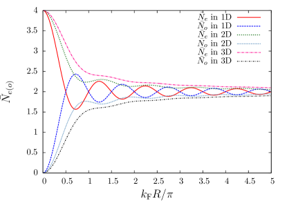
Figure 1: (Color online) Normalization constants $\bar{N}_{e(o)}$ for different dimensions $D$ vs the dimensionless distance $x=k_{\mathrm{F}}R/\pi$. For $R\rightarrow\infty$ $\bar{N}_{e}$ is equal to $\bar{N}_{o}$.

The spatial correlations depend on the dimensionality of the host. For a given distance $R$, the dimensionality enters primarily via the dimension of the wave vector $\vec{k}$ in the Eqs. (6) and the energy dispersion $\varepsilon_{\vec{k}}$ of the host.

In order to obtain information on generic spectral densities $N^{2}_{e(o)}(\epsilon)\rho(\epsilon)$ appearing in the Eqs. (8) and (9) we assume a isotropic linear dispersion $\epsilon_{\vec{k}}=v_{\mathrm{F}}\left(|\vec{k}|-k_{\mathrm{F}}\right)$, where $v_{\mathrm{F}}$ is the Fermi velocity and $k_{\mathrm{F}}$ the Fermi wave-vector. Inserting the dispersion in equations (6) yields in 1D to

$$N^{2}_{e(o)}(\epsilon)\rho(\epsilon)=2\rho_{0}\left[1\pm\cos\left(x\pi\left(1+\frac{\epsilon}{D}\right)\right)\right]$$ (17)

where $\rho_{0}=1/2D$ is the constant density of states and $x=k_{\mathrm{F}}R/\pi$. In higher dimensions we perform the angular integration to obtain for 2D

$$N^{2}_{e(o)}(\epsilon)\rho(\epsilon)=2\rho_{0}\left[1\pm J_{0}\left(x\pi\left(1+\frac{\epsilon}{D}\right)\right)\right]$$ (18)

with the zeroth Bessel function $J_{0}(x)$. In 3D, the effective densities of states Jones and Varma (1987); Jones et al. (1988) reads

$$N^{2}_{e(o)}(\epsilon)\rho(\epsilon)=2\rho_{0}\left[1\pm\frac{\sin\left(x\pi\left(1+\frac{\epsilon}{D}\right)\right)}{x\pi\left(1+\frac{\epsilon}{D}\right)}\right]\;\;.$$ (19)

Note that in 2D and 3D $\rho(\epsilon)$ is not constant for a linear dispersion, and $\rho(\epsilon)=\rho_{0}=1/2D$ is a simplification.

The normalization constants $\bar{N}_{e(o)}$ reveal important information on the admixture of even and odd bands for a given distance $R$. They are shown as a function of the dimensionless distance $x=k_{\mathrm{F}}R/\pi$ for different dimensions D in Fig. 1. Clearly, $\bar{N}_{o}(x=0)=0$ in any dimension: the odd band decouples from the problem, and the standard Kondo model is recovered which allows to calculate local ($R=0$) expectation values within the standard single band NRG .

With increasing $R$, the oscillations of the even and odd density of states $\rho_{e(o)}$ decay as $\propto R^{(1-D)/2}$. For large distances, the even and odd bands become equal and the normalization constants approach the same value. For 1D, strong oscillations are observed for short distances which are suppressed in higher dimensions. Apparently the $R$ dependence will be more pronounced in lower dimensions and the correlation function will decay with the different power law than in higher dimensions.

III Equilibrium physics: spatial correlation

III.1 Kondo regime: Short distance vs large distance properties

$\rho_{0}J$	$T_{\mathrm{K}}/D$	$k_{\mathrm{F}}\xi_{\mathrm{K}}$
$0.05$	$1\cdot 10^{-10}$	$1\cdot 10^{10}$
$0.075$	$1.7\cdot 10^{-7}$	$5.88\cdot 10^{6}$
$0.1$	$7.5\cdot 10^{-6}$	$1.33\cdot 10^{5}$
$0.15$	$3.9\cdot 10^{-4}$	$2564.10$
$0.3$	$0.0204$	$49.02$
$0.5$	$0.0749$	$13.35$
$0.6$	$0.115$	$8.69$
$0.7$	$0.2103$	$4.76$

Table 1: The Kondo temperature $T_{K}$ and length scale $\xi_{\mathrm{K}}$ for different Kondo couplings. The Kondo temperatures have been obtained from the NRG level flow - see text.

There are two characteristic length scales in the problem: $1/k_{F}$ defined by the metallic host, governing the power-law decay of $\chi_{\infty}(R)$ and its RKKY oscillations, and the Kondo length scale $\xi_{K}$, sometimes referred to as size of the Kondo screening cloud Barzykin and Affleck (1996, 1998); Affleck and Simon (2001); Sørensen and Affleck (2005); Affleck et al. (2008). Since $\xi_{K}$ increases exponentially with decreasing $J$, we use different $J$ to present data for the two different regimes $R<\xi_{K}$ and $\xi_{K}<R$. The results for $\chi_{\infty}(R)$ for these two different regimes are shown in Fig. LABEL:fig:2ab.

In our calculations, the Kondo temperature $T_{\mathrm{K}}$ has been defined from the NRG level flow: $T_{\mathrm{K}}$ is the energy scale at which the first excitation reaches $80$ % of its fixed point value. The Kondo temperature $T_{\mathrm{K}}$ and length scale $\xi_{\mathrm{K}}$ for different Kondo couplings are stated in Table. 1. All correlation functions have been obtained for $T/T_{\mathrm{K}}\to 0$. The sum rule (15) of $\chi_{\infty}(R)$ is numerically fulfilled up to typically 2% error in 1D.

In contrast to the original work by Borda Borda (2007), we observe ferromagnetic and anti-ferromagnetic correlations for short distances in accordance with predictions Barzykin and Affleck (1996, 1998); Affleck and Simon (2001); Sørensen and Affleck (2005); Affleck et al. (2008) by Affleck and his collaborators as presented in Fig. LABEL:fig:2ab(a). For distances $R\ll\xi_{\mathrm{K}}$, the impurity is still unscreened and impurity spin behaves more like a free spin. We have plotted the rescaled correlation function $R\chi_{\infty}(R)$ to reveal the $1/R$ decay at short distances in 1D Borda (2007) stemming from the analytical form of the RKKY interaction.

We have also added the RKKY interaction $K_{\mathrm{RKKY}}$ between the impurity spin and a fictitious probe impurity spin at distance $R$ obtained in second order perturbation theory for comparison (details of the calculations can be found in Appendix A). The oscillating part of $\chi_{\infty}(R)$, and the positions of the minima and maxima nicely agree with the RKKY interaction $\propto\cos(2k_{\mathrm{F}}R)$. For multiple integers $x=k_{\mathrm{F}}R/\pi=n$ the correlation function has minima and for odd multiple $x=n+1/2$ a maxima is found.

In order to access larger distances $R\gg\xi_{K}$, we increase $\rho_{0}J$. The rescaled spin correlation function $R^{2}\chi_{\infty}(R)$ depicted in Fig. LABEL:fig:2ab(b) clearly reveals the power-law decay of the envelop function at distances $R/\xi_{K}\gg 1$ as $1/R^{2}$. Furthermore, we only find antiferromagnetic correlations for $R/\xi_{K}\gg 1$, and $\chi_{\infty}(R)$ remains negative at all distances. In this regime, the maxima have the value $\chi_{\infty}(R)=0$ as noted earlier Barzykin and Affleck (1996, 1998); Affleck and Simon (2001); Sørensen and Affleck (2005); Affleck et al. (2008): The impurity spin is screened by the conduction band electrons and the envelope of $\chi_{\infty}(R)$ has to decreases faster.

We observe this crossover from a $1/R$ to a $1/R^{2}$ decay at around $R\approx\xi_{\mathrm{K}}$. We also find universal behavior for the envelope of $\chi_{\infty}(R)$ for distances $k_{\mathrm{F}}R/\pi>1$ and can reproduce Fig. 3 of Ref. Borda (2007) (not shown here.)

Since we have plotted $R^{2}\chi_{\infty}(R)$ which vanishes for $R=0$, the information of $\chi_{\infty}(0)$ is not included in the main panels of Fig. LABEL:fig:2ab. Therefore, we have added the $\rho_{0}J$ dependence of the local spin-correlation function $\chi_{\infty}(R=0)$ as inset to Fig. LABEL:fig:2ab(b). $\chi_{\infty}(0)<0$, as expected for a local antiferromagnetic coupling, and the strong coupling value of $-3/4$ is approached for large $J$: almost the whole contribution to the sum rule (15) is located in the first antiferromagnetic peak at $R=0$, and $\chi_{\infty}(R)$ has to decay very rapidly with increasing $R$.

In Fig. 3, the short distance behavior of $\chi_{\infty}(R)$ in 2D is shown. As for 1D case the oscillating part and the positions of the minima and maxima of $\chi_{\infty}(R)$ and the 2D RKKY-interaction nicely agree. In contrast to 1D, the RKKY interaction acquires a more complex mathematical structure even for a simplified linear dispersion replacing the simple $\cos(2k_{\mathrm{F}}R)$ oscillations in 1D. Therefore, modification to the $\cos(2k_{\mathrm{F}}R)$ behavior must be taken into account when analyzing experimental data.

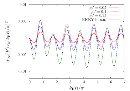
Figure 3: (Color online) The spin-correlation function $R^{2}\chi_{\infty}(R)$ as a function of the dimensionless distance $x=k_{F}R/\pi$ in 2D. In higher dimensions, the envelope of the RKKY and $\chi_{\infty}(R)$ has a more complicated structure. Every second maximum has a lower amplitude. NRG parameters are $\Lambda=5$ and $N_{s}=3000$.

III.2 Ferromagnetic couplings $J<0$ in 1D

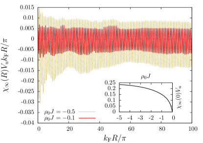
Figure 4: (Color online) The spin-correlation function $R\chi_{\infty}(R)$ as a function of the dimensionless distance $x=k_{\rm F}R/\pi$ in 1D for two different ferromagnetic Kondo couplings $\rho_{0}J=-0.1$ and $\rho_{0}J=-0.5$ for $T\to 0$. The inset shows $\chi_{\infty}(0)$ vs $\rho J$. For large ferromagnetic couplings $0.25$ is reached. NRG parameters are $\Lambda=3$ and $N_{s}=1400$.

Up until now, we have focused only on antiferromagnetic Kondo coupling causing the Kondo-singlet formation described by the strong-coupling (SC) fixed point for $T\to 0$. We extend our discussion of the equilibrium correlation function to the ferromagnetic regime characterized by the local-moment (LM) fixed point and a twofold degenerate ground state. As pointed out above, the sum rule for $\chi_{\infty}(\vec{r})$ predicts that the spatial integral of the correlation function vanishes. For a ferromagnetic coupling, $\xi_{\rm K}\to\infty$, and the correlation function is also oscillating as $\cos(2k_{\rm F}R)$ and decaying as $1/R$ for at all distances in 1D.

Exemplifying our findings, we depicted $R\chi_{\infty}(R)$ for two different Kondo coupling, $\rho_{0}J=-0.1$ and $\rho_{0}J=-0.5$, in Fig. 4. We numerically checked the sum rule and found deviations from zero by less than 1% in 1D. The RKKY oscillations and $1/R$ decay of the envelop function are clearly visible up very larger distances $k_{\rm F}R/\pi=100$.

In the ferromagnetic regime, the local spin-correlation function $\chi_{\infty}(0)$ must be positive and approaches its upper limit of $\chi_{\infty}(0)\to 1/4$ for $J\to-\infty$ as shown in the inset of Fig. 4. In order to fulfill the sum rule, $\chi_{\infty}(R)$ does not oscillate symmetrically around the $x$ axis: $\chi_{\infty}(R)$ must be slightly shifted to antiferromagnetic correlations to compensate the ferromagnetic peak at $R=0$.

IV Nonequilibrium dynamics

IV.1 Extension of the NRG to nonequilibrium: the TD-NRG

The TD-NRG has been designed Anders and Schiller (2005, 2006) to track the real-time dynamics of quantum-impurity systems following an abrupt quantum quench such as considered here; at $t=0$, we switch on the Kondo coupling $J$ between the prior decoupled impurity spin and the metallic host.

Initially, the entire system is characterized by the density operator of the free electron gas

$$\hat{\rho}_{0}=\frac{e^{-\beta H_{0}}}{{\rm Tr}\left[e^{-\beta H_{0}}\right]},$$ (20)

at time $t=0$ when the Kondo interaction $H_{K}$ is suddenly switched on: $H=H_{0}+H_{K}$. The density operator evolves thereafter in time according to

$$\hat{\rho}(t>0)=e^{-itH}\hat{\rho}_{0}e^{itH}.$$ (21)

Our objective is to use the NRG to compute the time-dependent expectation value $O(t)$ of a general local operator $\hat{O}$. As shown in Refs Anders and Schiller (2005, 2006), the result can be written in the form

$$\langle\hat{O}\rangle(t) = \sum_{m}^{N}\sum_{r,s}^{\rm trun}\;e^{it(E_{r}^{m}-E_{s}^{m})}O_{r,s}^{m}\rho^{\rm red}_{s,r}(m),$$ (22)

where $E_{r}^{m}$ and $E_{s}^{m}$ are the dimension-full NRG eigenenergies of the perturbed Hamiltonian at iteration $m\leq N$, $O_{r,s}^{m}$ is the matrix representation of $\hat{O}$ at that iteration, and $\rho^{\rm red}_{s,r}(m)$ is the reduced density matrix defined as

$$\rho^{\rm red}_{s,r}(m)=\sum_{e}\langle s,e;m|\hat{\rho}_{0}|r,e;m\rangle.$$ (23)

The restricted sum over $r$ and $s$ in (22) requires that at least one of these states is discarded at iteration $m$. The NRG chain length $N$ implicitly defines the temperature entering Eq. (20): $T_{N}\propto\Lambda^{-N/2}$, where $\Lambda>1$ is the Wilson discretization parameter.

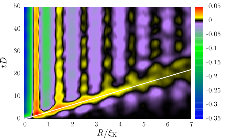
Figure 5: (color online) The 1D time and spatial dependent spin-correlation function $\chi(R,t)$ vs $x=k_{\rm F}R/\pi$ and $\tau=tD$ for $\rho_{0}J=0.3$ as a color contour plot. Its color map is depicted on the right site. The correlation propagates with $v_{\mathrm{F}}$, which is added as white line as guide to the eye. NRG parameters are $\Lambda=3$, $N_{s}=1400$ and $N_{z}=4$.

The derivation of Eq. (22) is based on the two observations. (i) It has been shown Anders and Schiller (2005, 2006) that the set of all discarded states in the NRG procedure forms a complete basis set of many-body Fock space which are approximate eigenstates of the Hamiltonian. (ii) The general local operator $\hat{O}$ is diagonal in the environment degrees of freedom (DOF) such that the trace over these DOF can be performed analytically yielding $\rho^{\rm red}_{s,r}(m)$. This approach has been extended to steady state currents at finite bias Anders (2008); Schmitt and Anders (2010); *SchmittAnders2011; Jovchev and Anders (2013). The only error of the method stems from the representation of the bath continuum $H_{0}$ by a finite-size Wilson chainWilson (1975) and are essentially well understood Eidelstein et al. (2012); Guettge et al. (2013).

IV.2 Time-dependent spatial correlation function in the Kondo regime

After discussing the equilibrium correlation function in Sec. III, we present our results for the full time-depended correlation function $\chi(\vec{r},t)$. The NRG fixed point differs for different signs of the Kondo coupling: for $J>0$ the SC fixed point Wilson (1975) is reached while for $J<0$ the system approaches the LM fixed point. Therefore, we present data for both regimes and begin with the antiferromagnetic Kondo coupling.

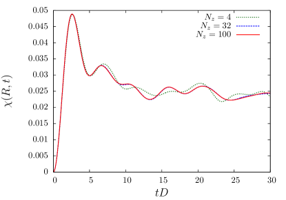
Figure 6: (color online) Time dependent correlation function $\chi(R,t)$ for a fixed distance $k_{F}R/\pi=0.51$ vs time for different number of $z$ averages $N_{z}$ and a fixed $\rho_{0}J=0.3$. NRG parameters are $\Lambda=3$ and $N_{s}=1600$.

$\chi(R,t)$ is depicted as a function of the dimensionless distance $x=k_{\rm F}R/\pi$ and the dimensionless time $\tau=tD$ for a moderate Kondo coupling $\rho_{0}J=0.3$ as a color contour plot for 1D in Fig. 5. Each distance $R$ requires a single TD-NRG run. Therefore, we have restricted ourselves to $N_{z}=4$ values for the $z$ averaging Yoshida et al. (1990); Anders and Schiller (2005, 2006) for the $N_{R}=350$ different values of $R$ included in Fig. 5 and only kept a moderate number of NRG states.

The development of the ferromagnetic correlation maximum at $x=1/2$ is clearly visible already after very short times corresponding to $\chi_{\infty}(R)$ depicted in Fig. LABEL:fig:2ab(a). For $t\to\infty$, the equilibrium Friedel oscillations as discussed above are recovered: the correlation function has minima for $x=n$, and maxima are found for odd multiple $x=n+1/2$. For larger distances and times the ferromagnetic correlations are suppressed in favor of purely antiferromagnetic correlations as expected from the equilibrium correlation function.

After the ferromagnetic correlation maximum has passed, $\chi(R,t)$ exhibits some weak oscillations in time for $R=$ const. In order to discriminate between finite size oscillations caused by the bath discretiation Anders and Schiller (2006); Eidelstein et al. (2012); Guettge et al. (2013) and the real nonequilibrium dynamics of the continuum, the time evolution of $\chi(R=0.51\pi/k_{\rm F},t)$ is shown for different number of z-averages $N_{z}$ in Fig. 6. Since the short-time oscillations clearly converge with increasing $N_{z}$, they contain relevant real-time dynamics which will be analysed in more detail in the next section below. In the long-time limit, the TD-NRG oscillates around a time average, which is independent of $N_{z}$, and is close to the equilibrium correlation function $\chi_{\infty}(R)$. Those oscillations are partially related to the bath discretisation Anders and Schiller (2006); Eidelstein et al. (2012); Guettge et al. (2013) and are be suppressed for increasing number of $z$ values $N_{z}$, decreasing $\Lambda$ and increasing number of $N_{s}$. Therefore, we conclude that thermodynamic equilibrium is reached up to the well understood small discretisation errors Anders and Schiller (2006); Eidelstein et al. (2012); Guettge et al. (2013).

IV.2.1 How are the Kondo correlation building up at different distances $R$ with time?

Clearly visible is the propagation of ferromagnetic correlations away from the impurity with a constant velocity given by the Fermi velocity of the metallic host. At the impurity site, an antiferromagnetic spin-spin correlation develops rather rapidly. Since the total spin is conserved in the system, a ferromagnetic correlation-wave propagates spherically away from the impurity spin. The added white line $R=v_{\rm F}t$ serves as guide to the eye in Fig. 5 to illustrate this point. This line represents the analog to a light cone in electrodynamics.

Inside the light cone, the equilibrium correlation function is reached rather fast. To exemplify this, we plot $\chi(R,t)$ as function of relative time $t^{\prime}=t-R/v_{\rm F}$ for four different distances $R$ in Fig. LABEL:fig:chi-r-t-fixed-R(a). Negative $t^{\prime}$ corresponds to the correlations outside the light cone, while for $t^{\prime}>0$ the spin correlation function $\chi(R,t)$ inside the light cone is depicted.

At the origin of the impurity ($R=0$), a antiferromagnetic correlation develops on the time scale $1/\sqrt{J}$: the short time dynamics is linear in the Kondo coupling and proportional to $t^{2}$ as will be discussed in greater detail below.

At $t^{\prime}=0$ and finite distance $R>0$, a significant ferromagnetic correlation-wave peak is observe which decays rather rapidly. Its position corresponds to the yellow (color-online) light cone shown in Fig. 5. In order to shed some light into the nature of this rapid decay, we present the ratio $\chi(R,t)/\chi_{\mathrm{max}}$ versus $(t-t_{\mathrm{max}})D$ for a constant distance $k_{\mathrm{F}}R/\pi=2.01$ and different couplings $\rho_{0}J$ in Fig. LABEL:fig:chi-r-t-fixed-R(b). $\chi_{\mathrm{max}}$ has been defined as $\chi_{\mathrm{max}}=\chi(R,t_{\mathrm{max}})$, and $t_{\mathrm{max}}$ is the numerical position of the ferromagnetic peak. Note that $t_{\mathrm{max}}$ slightly differs from bare light cone time scale $R/v_{\mathrm{F}}$ and is shifted to larger times with increasing $\rho_{0}J$ (not shown.) This increasing shift can be analytically understood, and we will give the detailed explanation in Sec. IV.3 below. After dividing out the amplitude $\chi_{\mathrm{max}}$ of the maximum, the decay surprisingly shows a universal behavior and the time scale is simply given by $1/D$. A comparision of the oscillation with $\cos(t^{\prime}D)$ (pink dash-dotted line) shows a remarkable agreement for small times $0<t^{\prime}D<1$. This indicates that the functional form of $\chi(R,t)$ for fixed $R$ consists of a damped oscillatory $\cos(t^{\prime}D)$ term whose maximum is reach when the ferromagnetic correlation wave reaches the distances $R$ at the time $t_{\rm max}>R/v_{\rm F}$. For larger times $t^{\prime}$, $\chi(R=2.01\pi/K_{\rm F})$ has to approach an finite antiferromagnetic value. Therefore, the oscillations in the TD-NRG are not centered around the origin but shifted to negative values as can seen in Fig. LABEL:fig:chi-r-t-fixed-R(b) by comparing with the undamped $\cos(t^{\prime}D)$ curve.

Most striking, however, is the building up of correlations for $t^{\prime}<0$ outside of the light cone. These correlations are antiferromagnetic and show no exponential decay. These correlations appear shortly before the light cone. They reach their largest modulus for odd multiple $k_{\mathrm{F}}r/\pi=n+1/2$ and decay with a power law as $tD$ goes to zero. In Sec. IV.4 below, we will provide a detailed analysis of their origin and present an analytically calculation in $J$ that agrees remarkably well with the observed TD-NRG results.

Such a building up of correlations outside of the light cone has recently be reported in a perturbative calculations Medvedyeva et al. (2013) neglecting, however, the $2k_{\rm F}$ oscillations. Here, we present results for a full nonperturbative calculation which includes the Friedel oscillations containing the RKKY mediated effective spin-spin interaction.

The different behavior for short and long distances is illustrated in Fig. LABEL:TD_xi_Kl. The upper panel shows results for short distances $r/\xi_{\mathrm{K}}\ll 1$. We observe the distinctive ferromagnetic correlation which propagates with the Fermi velocity through the conduction band. Inside the light cone, we find oscillations between ferromagnetic and antiferromagnatic correlations. In the lower panel, the behavior for longer distances is depicted. We find that the ferromagnetic propagation vanishes at around $k_{\mathrm{F}}R\approx\xi_{\mathrm{K}}$. At these distances, we only observe oscillations between zero and antiferromagnatic correlations inside the light cone. For both cases, the long-time behavior agrees remarkable well with the NRG equilibrium calculations.

IV.3 Perturbation theory

Surprisingly, we found in our TD-NRG results the building up of spin-correlations outside of the light cone which do not decay exponentially. In order to rule out TD-NRG artifacts and shed some light into its origin, we perturbatively calculate $\langle\vec{S}_{\rm imp}\vec{s}(r)\rangle(t)$ up to second order in $J$.

Since only $H_{0}$ enters the initial density operator, we transform all operators into the interaction picture and, after integrating the von Neumann equation, we obtain for the density operator

$$\rho^{I}(t) \approx \rho_{0}+i\int_{0}^{t}\left[\rho_{0},H_{K}^{I}(t_{1})\right]dt_{1}$$ (24)

$$-\int_{0}^{t}\int_{0}^{t_{1}}\left[\left[\rho_{0},H_{K}^{I}(t_{2})\right]H_{K}^{I}(t_{1})\right]dt_{2}dt_{1}$$

which is exact in second order in the Kondo coupling $J$. The superscript $I$ labels the operators in interaction picture $A^{I}(t)=e^{iH_{0}t}Ae^{-iH_{0}t}$, and the boundary condition is given by $\rho_{0}=\rho^{I}(t=0)$. We use this $\rho^{I}(t)$ to calculate the spin-spin correlation function

$$\chi(\vec{r},t) = {\rm Tr}\left[\rho^{I}(t)\vec{S}_{\rm imp}\vec{s}^{I}(\vec{r},t)\right]$$ (25)

where only expectation values with respect to the initial density operator $\rho_{0}$ enter. The occurring commutators are cumbersome but can be evaluated analytically (for details see Appendix B). We note that the contribution in linear order in $J$ does not vanish for a perturbation $H_{K}=J\vec{S}_{\rm imp}\vec{s}(0)$. Although the time integrals can be performed analytically, the multiple momenta integrations of the free conduction electron states must be performed numerically.

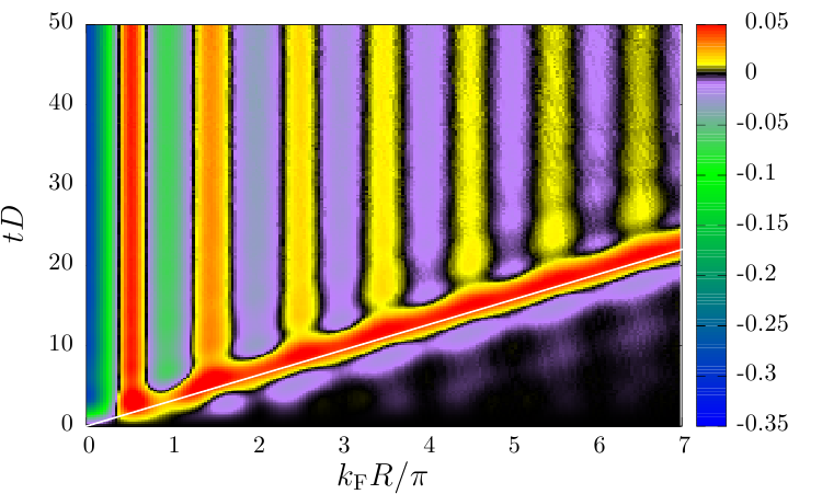
Figure 9: (Color online) The analytical $\chi(R,t)$ evaluated numerically for $\rho_{0}J=0.3$ up to second order in $J$ as a color contour plot. Its color map is depicted on the right site. The light cone $R=v_{\mathrm{F}}t$ has been added as a white line.

The sum of the first- and second-order contributions to $\chi(R,t)$ are shown in Fig. 9 up to relatively large times. This perturbatively calculated $\chi(R,t)$ turns out to be well behaved and does not contain secular terms. Clearly, the Kondo physics is not included in such an approach remaining only valid for $r/\xi_{\mathrm{K}}\ll 1$ and $tT_{K}\ll 1$. Therefore, we expect deviations at large distances and times from the NRG results.

Nevertheless, the NRG result depicted in Fig. 5 and the perturbation theory result qualitatively agrees very well. As in the TD-NRG, ferromagnetic correlations propagate spherically away from the impurity with Fermi velocity (white line as guide to the eye) in the perturbative solution. For long times an equilibrium is reached: we recover the distance dependent Friedel oscillations which are known from the RKKY interaction. We also find the same antiferromagnatic correlations outside the light cone as in the NRG results. Again, their maxima are located at odd multiple of $x=k_{\mathrm{F}}R/\pi=n+1/2$ at the same positions as predicted in the TD-NRG calculations.

To the leading order in the Kondo coupling $\rho_{0}J$, the ferromagnetic wave in the correlation function propagates on the light cone line $R=v_{\rm F}t$. Note, however, that the peak position of the analytical $\chi(R,t)$ plotted in Fig. 9 is slightly shifted to later times than defined by the light cone line. This shift coincides with the one observed in the TD-NRG results shown in the Figs. 5 and LABEL:fig:chi-r-t-fixed-R. With our analytical analysis at hand, we can provide a detailed understanding of this effect. The first-order contribution given by Eq. (46) yields a peak of ferromagnetic correlations positioned exactly on light cone line. However, the maximum of the second-order contribution (47) is shifted to slightly larger times. Adding both contributions generates a $J$-dependent line for the ferromagnetic peak position away from the light cone line: the larger $J$, the later the ferromagnetic maximum occurs due to increasing importance of the second order contribution.

While these spatial oscillations are implicitly encoded in the effective even and odd density of states in the NRG calculation, they are explicitly generated by the momenta integration in the perturbative approach. This confirms our TD-NRG results and provides a better understanding of the numerical data.

Comparing Figs. 5 and 9 in more detail illustrates the shortcomings of the perturbative approach which remains only valid for $R/\xi_{\mathrm{K}}\ll 1$. As discussed in Sec. III above , the decay of the envelope function crosses over from a $1/R$ to an $1/R^{2}$ behavior due to the Kondo screening of the local moment for $R/\xi_{\rm K}>1$. Since the perturbative approach is unable to access the Kondo-singlet formation the perturbative solution depicted in Fig. 9 decays as $1/R$ at all distances and also remains oscillating between ferromagnetic and antiferromagnetic correlations while the TD-NRG correctly predicts only antiferromagnetic correlations inside the light cone once $R$ exceeds the Kondo length scale $\xi_{\rm K}$.

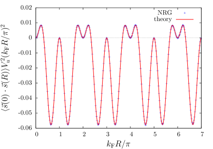
Figure 10: (Color online) The intrinsic spin-spin correlations of the Fermi sea between the spin densities $\vec{s}(0)$ and $\vec{s(r)}$ in 1D. Via the mapping to the even and odd conduction bands we are able to measure bath properties at distance $R$ and get a perfect agreement between theory and NRG results. NRG parameters are $\Lambda=3$ and $N_{s}=1200$.

IV.4 Intrinsic correlations of the Fermi sea

Since the perturbative results agree remarkably well with the TD-NRG data for short distances, the analytical approach can be used to gain an explicitly understanding of the correlations outside of the light cone. It has been proposed Medvedyeva et al. (2013) that these correlations originate from the intrinsic spin-spin correlations in the Fermi sea $\langle\vec{s}(0)\vec{s}(\vec{r})\rangle$ already present prior to the coupling of the impurity. Once the impurity is coupled to the local conduction electron spin density at time $t=0$, we instantaneously probe these intrinsic entanglements of the Fermi sea between the local spin density and the spin density at a large distance $R$.

For $J=0$, $\langle\vec{s}(0)\vec{s}(R)\rangle$ can be calculated analytically and is given by

$$\langle\vec{s}(0)\vec{s}(R)\rangle = \frac{3\sin(k_{\mathrm{F}}R)\sin(\frac{k_{\mathrm{F}}R}{2})\cos(\frac{3}{2}k_{\mathrm{F}}R)}{4V_{u}^{2}(k_{\mathrm{F}}R)^{2}}$$ (26)

in 1D. This exact result coincides with the NRG data obtained by setting $J=0$ in an equilibrium NRG calculation as shown in Fig. 10. This excellent agreement between the analytical and the NRG approaches serves as further evidence for the numerical accuracy of mapping Eqs. (7)-(9) to the two discretized and properly normalized Wilson chains for even and odd parity conduction bands.

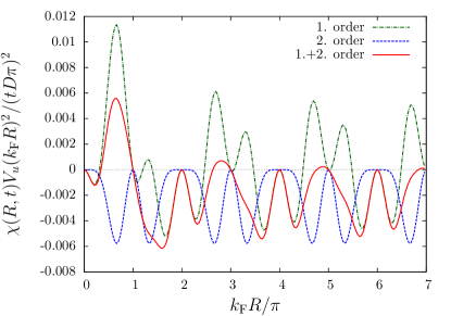
Figure 11: (Color online) First and second order of $\chi(R,t)$ for small times $t$ and $\rho_{0}J=0.3$ in 1D. Even for short times we observe correlations for large distances. A comparison with a) shows that the positions of these correlations coincide with the positions of the intrinsic correlations of the Fermi sea. So the correlations outside the light cone originate from these intrinsic correlations.

In order to connect the intrinsic spin entanglement of the decoupled Fermi sea with the observed antiferromagnetic correlations outside of the light cone, we expand the perturbative calculated $\chi(R,t)$ for small times $0\leq tD\ll 1$ and perform the momentum integrations analytically, separately for the first and the second order contributions.

The leading order terms in time are proportional to $\propto(tD)^{2}$ and decay as $1/R^{2}$. We recall the difference between the $1/R^{2}$ decay outside of the light cone for the short-times dynamics and the well understood $1/R$ decay inside the light cone when the equilibrium reached. Therefore, we have plotted the perturbative results in 1D as $\chi(R,t)(R/(tD))^{2}$ in Fig. 11 to eliminate the time dependence and compensate for the leading spatial decay of the envelop function. The first-order contribution (green online) is shown as a dashed-dotted line, the second-order contribution (blue online) is depicted as a dashed line, and the sum of both (red online) is added as a solid line for $\rho_{0}J=0.3$ in Fig. 11.

Since the second-order contribution to $\chi(0,t)$ remains always zero in a short-time expansion, the time evolution of the antiferromagnetic correlation at $R=0$ is dominated by the first-order term being proportional to $\propto Jt^{2}$. Therefore, the time scale for the initial fast buildup of the local antiferromagnetic correlation is given by $1/\sqrt{J}$ confirming the TD-NRG short-time dynamics for $k_{\rm F}R/\pi=0.01$ as depicted in Fig. LABEL:fig:chi-r-t-fixed-R(a).

The largest contribution for short times stems from the ferromagnetic peak around $k_{\mathrm{F}}R/\pi=0.5$. However, correlations are visible at all length scales which develop quadratically in time. The positions of the maxima and minima agree remarkable with those of the intrinsic correlation function $\langle\vec{s}(0)\vec{s}(R)\rangle$ of the Fermi sea depicted in Fig. 10 and both decay with $1/R^{2}$.

Since the first-order contribution is sensitive to the sign of $J$, its maxima contribute with the equal sign as $\langle\vec{s}(0)\vec{s}(R)\rangle$ for ferromagnetic $J$ and opposite sign for an antiferromagnetic coupling. The second-order term only adds negative (antiferromagnetic) contributions to $\chi(R,t)$. The location of its negative peaks coincide with the antiferromagnetic peak location of the spin-spin correlation function $\langle\vec{s}(0)\vec{s}(\vec{r})\rangle$ of the decoupled Fermi sea depicted in Fig. 10. The sum of both orders contains only small ferromagnetic correlations for larger distances $k_{\mathrm{F}}R/\pi>1$ for $\rho_{0}J=0.3$. The larger the coupling $J$ is the smaller these ferromagnetic correlations are due to the increasing dominance of the second-order term.

We can conclude from this detailed analytical analysis that the antiferromagnetic correlation directly in front of the light cone results from the antiferromagnetic peak in the intrinsic correlations from the Fermi sea at around $k_{\mathrm{F}}R\approx 1.6\pi$. This peak also propagates through the conduction band with the Fermi velocity. Because the intrinsic correlations decay with $1/(k_{\mathrm{F}}R)^{2}$, the propagation of the antiferromagnetic peaks for larger distances is not visible.

IV.5 Local moment regime: ferromagnetic coupling: $J<0$

Now we extend the discussion to ferromagnetic Kondo couplings. In this regime, the LM fixed point is stable, and the ground state is two fold degenerate in the absence of an external magnetic field. In the RG process, the Kondo coupling is renormalized to zero. Nevertheless, the spatial spin-correlation function $\chi_{\infty}(R)$ remains finite for $T\to 0$ as discussed in Sec. III.2.

The results for the time-dependent spin-correlation function $\chi(R,t)$ are shown as a color contour plot in Fig. LABEL:fig:chi-ferro-j03. Figure LABEL:fig:chi-ferro-j03(a) depicts the TD-NRG calculation, while the analytical result obtained up to the second-order perturbation theory is added as panel (b) for the same parameters. Since the first-order contribution is sign sensitive, the analytical correlation function differs significantly from the antiferromagnetic regime displayed in Fig. 9.

As in the Kondo regime, the analytical and the TD-NRG results agree qualitatively very well. The Friedel oscillations with the frequency $2k_{\rm F}$ are clearly visible inside the light cone. Note the phase shift compared to the Kondo regime: now the ferromagnetic correlations are observed at $x=n$ and the antiferromagnetic correlations at half integer values of $x$.

Since a ferromagnetic correlation is building up at the impurity spin position on a very short time scale $\propto 1/\sqrt{J}$, and the total spin of the system is conserved, an antiferromagnetic correlation wave spherically propagates away from the origin traveling with the Fermi-velocity $v_{\rm F}$ (again we have added a white line $R=v_{\rm F}t$ as guide to the eye to both panels). For ferromagnetic couplings the peak position of the propagation is slightly shifted to earlier times $t_{\mathrm{max}}<R/v_{\mathrm{F}}$, due to the sign change of the first-order contribution. The correlations outside the light cone are stronger suppressed compared to the Kondo-regime. Again, we can trace the origin to the intrinsic entanglement of the Fermi sea by consulting Figs. 10 and 11 as well as the discussion above.

IV.6 Finite temperature: cutoff of the Kondo correlations

Up to now, we have only considered the zero-temperature limit. Next, we extend the discussion to the propagation of the correlations at finite temperatures.

Figure LABEL:fig:finitetemp illustrates the difference in the time-dependent correlation function at the two different temperatures $T=0$ and $T=2T_{\mathrm{K}}$, depicted in panels (a) and (b), respectively. Note that we have used the data of Fig. 5 but measure the distance $R$ in units of the Kondo correlation length $\xi_{\mathrm{K}}$.

For both temperatures, we observe the correlations in and outside of the light cone and the propagation of the ferromagnetic correlation with Fermi velocity as described in Sec. IV.2. While for small distances $R/\xi_{\mathrm{K}}\leq 0.15$, the spin-correlation functions agree well for both temperatures, the correlations inside and outside of the light cone become strongly suppressed in the finite temperature data once $R$ exceeds $0.5\xi_{\mathrm{K}}$: the correlations are cut off at the thermal length scale $\xi_{\mathrm{T}}=v_{\mathrm{F}}/T=v_{\mathrm{F}}/(2T_{\mathrm{K}})=0.5\xi_{\mathrm{K}}$.

The ferromagnetic correlation which propagates with Fermi velocity, however, is amplified due to spin conservation. Because of the strong suppression outside of the light cone, the total spin has to be distributed over a larger area.

Figure 14 shows the approach to the equilibrium correlation functions at large times: the spatial dependence of the spin correlation functions for both temperatures is plotted using the data of Fig. LABEL:fig:finitetemp at the largest time $D=70$. In the $T=0$ curve (dashed line), the RKKY type of oscillations between anti-ferromagnetic and ferromagnetic peaks for small distances and only antiferromagnetic correlations for larger distances are clearly visible. The decay of its envelope functions plotted as an inset of Fig. 14 reveals the power-law decay with the distance.

For the finite temperature $T=2T_{\mathrm{K}}$, however, the correlations are cut off, and, due to the rapid decay, only a few oscillations (solid red line) can be observed. The envelope in the inset shows the expected exponential decay at short distances. At larger distances, the numerical noise of the TD-NRG exceeds the rapid suppression of the correlation function, and one needs to resort to the equilibrium NRG (see Fig. 3 in Ref. Borda (2007)).

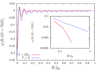
Figure 14: The correlation function $\chi(R,tD=70)$ vs $x=R/\xi_{\mathrm{K}}$ for the medium coupling $\rho_{0}J=0.3$ and the constant time $tD=70$ in 1D. For $T=0$ the RKKY like oscillations are observed while for $T=2T_{\mathrm{K}}$ the correlations are cut off.
The inset shows the envelope function of $\chi(R,tD=70)$.

V Response function

Within the linear-response theory, we can investigate the the conduction electron spin-density polarization $\langle\vec{s}(R,t)\rangle$ as a function of an externally applied local magnetic field $\vec{B}(t)$. Since the Kondo Hamiltonian is rotational invariant in spin space, the retarded spin-spin susceptibility tensor is diagonal and proportional to the unity matrix. Therefore, it is sufficient to investigate the conduction electron spin-density polarization in $z$ direction $\langle s^{z}(R,t)\rangle$ at distance $R$ of the Kondo spin caused by applying a local magnetic field $\vec{B}(t)=B(t)\vec{e}_{z}$ acting on the Kondo spin with $\vec{e}_{z}$ being the unity vector in $z$ direction.

The spin-density polarization $\langle\vec{s}(R,t)\rangle$

$$\langle s^{z}(R,t)\rangle = \langle s^{z}(R,t=-\infty\rangle$$ (27)

$$+\int_{-\infty}^{\infty}dt^{\prime}\,\chi^{r}_{\rm imp-c}(R,t-t^{\prime})\Delta(t^{\prime})\,,$$

is related to the retarded spin susceptibility

$$\chi^{r}_{\rm imp-c}(R,t) = -i\langle[s^{z}(R,t),S^{z}_{\rm imp}]\rangle\Theta(t)$$ (28)

that is a true response function. Since the system is unpolarized at $t=-\infty$, $\langle s^{z}(R,t=-\infty\rangle=0$ and can be neglected. In Eq. (27) the local applied time-dependent Zeeman splitting $\Delta(t)=g\mu_{B}B(t)$ has entered. Since the spin-density $s^{z}(R,t)$ and $S^{z}_{\rm imp}$ are Hermitian operators, $\chi^{r}(R,t)$ is a purely real function depending only on the spectrum Peters et al. (2006) $\rho^{r}_{\rm imp-c}(R,\omega)=-\lim_{\delta\to 0^{+}}\Im\chi^{r}_{\rm imp-c}(R,\omega+i\delta)/\pi$:

$$\chi^{r}_{\rm imp-c}(R,t) = -2\int_{0}^{\infty}d\omega\rho^{r}_{\rm imp-c}(R,\omega)\sin(\omega t)\,.$$ (29)

V.1 Retarded host susceptibility $\chi^{r}_{\rm c-c}(R,t)$

The retarded equilibrium host spin-density susceptibility

$$\chi^{r}_{\rm c-c}(R,t) = -i\langle[s^{z}(R,t),s^{z}(0,t)]\rangle\Theta(t)$$ (30)

can be analytically calculated in the absence of a coupling to the impurity ($J=0$) (see Appendix C). For a 1D linear dispersion, we have obtained

$$\rho^{r}_{\rm c-c}(R,\omega)= \frac{1}{2\pi V_{u}^{2}N^{2}}\sum_{k_{1},k_{2}}[f(\epsilon_{k_{2}})-f(\epsilon_{k_{1}})]$$ (31)

$$\times\left[\pi\cos((k_{2}-k_{1})R)\delta(\omega-(\epsilon_{k_{1}}-\epsilon_{k_{2}}))\right.$$

$$+\left.\frac{\sin((k_{2}-k_{1})R)}{\omega-(\epsilon_{k_{1}}-\epsilon_{k_{2}})}\right]\;\;.$$

The analytic expression (31) of the spin-spin susceptibility contains the dimensionless frequency $k_{F}R$ for a linear dispersion causing increasing frequency oscillations with increasing $R$.

The numerical effort for a calculation of these retarded spin-spin susceptibilities and their spectral functions using the NRG grows exponentially at larger distances since the high-energy spectrum of the NRG response function is much less accurate than its low-frequency counterpart. While the analytical calculation makes full use of the bath continuum, the conduction band is discretized on a logarithm energy scale Wilson (1975) and comprise only a few bath sites representing the high energy spectrum. Note that the NRG is geared towards the calculation of the impurity properties, while we are using the NRG to extract a bath correlation function. Therefore, we are limited to short distances for the bath spectral resolution in the NRG calculation.

To illustrate this point, we present a comparison between the analytical and the NRG spectral function as a benchmark in Fig. LABEL:fig:spin-spin-sus(a). While the agreement between the two results is very good at short distances, significant deviations are observed at $k_{\rm F}R/\pi=2.01$. Their origin can be traced to the limitation of the NRG to accurately resolve the high-energy part of the oscillations in the spectrum. The frequency scale of these oscillations is of the order of the band width $D$ as can be seen from Eq. (31). These high-energy oscillations cannot be properly resolved for large $R$ by the finite number of excitation energies provided by the NRG in this frequency range for a finite $\Lambda>1$. The low-energy part of the spectrum, however is excellently recovered by the NRG as expected.

After benchmarking the accuracy of the spectral functions at small distances, we have used the Fourier transformation Eq. (29) and the corresponding version for $\chi^{r}_{\rm c-c}(R,t)$ to calculate the retarded spin susceptibility in the time domain. A time-dependent and spatial conduction electron spin density $\langle s^{z}(R,t)\rangle$ is induced as a response to a fictitious local Zeeman splitting $\Delta(t)=g\mu_{\rm B}B\theta(t)$ applied locally at the origin.

We compare $\langle s^{z}(R,t)\rangle$ obtained from the NRG retarded spin-spin susceptibility $\chi^{r}_{\rm c-c}(R,t)$ (dashed line) and the analytical susceptibility (solid line) in Fig.  LABEL:fig:spin-spin-sus(b) Both susceptibilities have been calculated using the Fourier transformation of the data depicted in Fig.  LABEL:fig:spin-spin-sus(a) and substituting the resulting $\chi^{r}_{\rm c-c}(R,t)$ for $\chi^{r}_{\rm imp-c}(R,t)$ in Eq. (27). We have plotted $\langle s^{z}(R,t)\rangle$ normalized to the Zeeman energy $\Delta_{0}=g\mu_{\rm B}B$ to eliminate the trivial proportionality to the applied field strength.

The induced time-dependent spin-density polarization $\langle s^{z}(R,t)\rangle$ can be understood as a response to a spin wave propagating with the speed $v_{\rm F}$ through the lattice and a consecutive fast equalization. The maximum of the spin wave is expected to be found at the time $\tau_{l}=R/v_{\rm F}$ indicated by the arrows in Fig. LABEL:fig:spin-spin-sus(b). The analytical response can be evaluated at arbitrary distances $R$. Indeed, the center of the propagating spin wave is located exactly at the time $\tau_{l}$ for larger distances $k_{\rm F}R/\pi\geq 2$—not explicitly shown here—while for shorter distances we observe a slight shift as depicted in Fig. LABEL:fig:spin-spin-sus(b). Some response is found outside of the light cone related to the finite width of the spin wave. This finite spatial resolution is directly linked to the finite momentum cutoff in the analytical formula defined by the restriction of the $k$-values to the first Brillouin zone: a sharp suppression of the signal outside the light cone would require sending the momentum cutoff to infinity as done in the analytical calculation of Ref. Medvedyeva et al., 2013.

The spin-wave obtained from the NRG calculations is slightly faster originating from the shift of spectral weight to higher energies due to NRG spectral broadening Bulla et al. (2008) of the finite size NRG spectra as illustrated also in Fig. LABEL:fig:spin-spin-sus(a).

By comparing the numerical response with its analytical counterpart it is apparent that the small oscillations around the long time limit of the spin-density polarization are not a numerical artefact due to the NRG discretization errors but related to the finite bandwidth and the linear conduction band dispersion.

Furthermore, we find a significant deviation between the long-term limit of the spinpolarization calculated analytically and the one using the convolution of the NRG retarded susceptibility for $k_{\rm F}R/\pi=0.01$. It is straightforward to see that the stationary value is determined by the integral over $\rho^{r}_{\rm c-c}(R,\omega)/\omega$. As discussed above and depicted in Fig. LABEL:fig:spin-spin-sus(a), the finite resolution and the NRG broadening shifts some spectral weight to higher frequencies compared to the exact solutions, and, hence, we find a reduced value for $|\langle s^{z}(R\to 0,\infty)\rangle|$ since $\rho^{r}_{\rm c-c}(0,\omega)/\omega$ does not change sign. Once the spectral functions exhibit sign changes, broadening and finite size errors partially cancel and the accuracy of $\langle s^{z}(R,\infty)\rangle$ increases for larger $R$.

V.2 Retarded susceptibility $\chi^{r}_{\rm imp-c}(R,t)$

Now we proceed to the spin susceptibility $\chi^{r}_{\rm imp-c}(R,t)$ for finite $J$ describing the response of the conduction band spin-density at some distance $R$ to a perturbative magnetic field in $z$ direction coupling only to the impurity spin. Its spectral function is shown in Fig. LABEL:fig:spin-spin-response(a) for four different distances $R$ to illustrate the changes due to the presence of the Kondo spin ($J>0$).
Clearly, the increase of the numbers of oscillations in the frequency spectra with increasing $R$ prevails the indication of the RKKY mediated spin response. Furthermore, the antiferromagnetic coupling $J>0$ leads to a change of sign in $\rho^{r}_{\rm imp-c}$ compared to $\rho^{r}_{\rm c-c}$. A significant spectral weight is now located at low frequencies: the Kondo physics is reflected in the distinctive peak at $\omega\approx T_{\mathrm{K}}$ apparent for all distances $R$.

In Fig. LABEL:fig:spin-spin-response(b), the time dependence of the spin-density $\langle s^{z}(R,t)\rangle$ is shown for a Zeeman splitting $\Delta(t)=g\mu_{\mathrm{B}}B\theta(t)$ applied to the impurity spin. Compared to $\rho^{r}_{\rm c-c}$, one observes a change of sign in the response due to the antiferromagnatic coupling. For even multiples of $k_{\rm F}R/(2\pi)$, the conduction-band electron spin density aligns antiparallel, and for odd multiples the density aligns parallel to the impurity spin in the long-time limit reflecting the RKKY mediated spin response.

We have identified two relevant time scales in the induced spin density $\langle s^{z}(R,t)\rangle$: the fast light cone time scale $\tau=R/v_{\rm F}$ and the slow Kondo time scale $1/T_{K}$. The spin-density polarization remains almost zero until the ferromagnetic spin wave has propagated from the impurity spin to the distance $R$ after that $\langle s^{z}(R,t)\rangle$ starts building up [see inset of Fig. LABEL:fig:spin-spin-response(b)]. Again, the finite width of this spin-wave response is directly linked to the finite momentum cutoff of our single symmetric conduction band used in the NRG calculation as discussed above. The steady state, however, is reached very slowly: its sign is determined by the $R$-dependent RKKY interaction, and the long-time approach is governed by the Kondo scale $T_{K}$ independent of the distance as demonstrated in Fig. LABEL:fig:spin-spin-response(b). This is in contrast to the fast response of the decoupled Fermi sea, where the equilibrium spin polarization is reached rather fast on the time scale $1/D$ as depicted in Fig. LABEL:fig:spin-spin-sus(b).

To gauge the quality of the long-time steady-state value obtained within the linear-response theory, we have used an equilibrium NRG approach to calculate the equilibrium value $\langle s^{z}(R,\infty)\rangle/(g\mu_{\mathrm{B}}B)$ at a very small magnetic field $g\mu_{\mathrm{B}}B/D=10^{-8}$ acting on the impurity spin. These values are added as a horizontal line on the right of Fig. LABEL:fig:spin-spin-response(b). For vanishing local magnetic field, the linear response theory becomes exact, and the steady-state value must coincide with the equilibrium expectation value in an infinitely large system. Similar to Fig LABEL:fig:spin-spin-sus(b), the steady-state value $|\langle s^{z}(R,\infty)\rangle|$ calculated from the spectral function is smaller than the equilibrium value caused by the NRG broadening shift of spectral weight to higher energies. This origin of the deviations has already been discussed in Sec. V.1.

VI Discussion and outlook

We presented a comprehensive study of the spatial and temporal propagation of Kondo-correlations for antiferromagnetic and ferromagnetic Kondo couplings using the TD-NRG.

Our approach is based on a careful construction of two Wilson chains obtained from the two distance dependent even and odd parity bands. Full energy dependence and the correct normalization of the bands are required for accurate results. We have benchmarked our mapping by (i) calculating the intrinsic spatial dependence of spin-spin correlation of the Fermi sea, which coincides with the exact analytical calculation for the full continuum, and (ii) checking the sum rule of the equilibrium spin correlation function for ferromagnetic and antiferromagnetic couplings. Our numerical data fulfill the sum rule with an error of 1% in 1D, which provided a second independent check of the distance dependent NRG mapping.

The light cone defined by the Fermi velocity $R=v_{\rm F}t$ divides the parameter space of the spatial and temporal correlation function $\chi(R,t)$ in two segments. Inside the light cone, the spin correlations develop rather rapidly, and then are followed by a much slower decay towards the equilibrium correlation function. Typical decaying Friedel oscillations with a characteristic frequency $2k_{\rm F}$ are observed in the spatial dependence. In the Kondo regime, the envelope function shows a power-law behavior $1/R$ in equilibrium with ferromagnetic and antiferromagnetic correlations for short distances and crosses over to a $1/R^{2}$ behavior for distances exceeding the Kondo length scale $R>\xi_{\rm K}$ in 1D. In this region only antiferromagnetic correlations are found that correspond to a finite negative value of the sum rule.

For the ferromagnetic regime, the inverse length scale $1/\xi_{\rm K}$ vanishes, and the correlation function remains oscillatory with a slower decay of the envelope function. The position of minima and maxima are interchanged. The analytical calculation of the correlation function provides an excellent understanding of our numerical TD-NRG data.

Remarkably, we have found a building up of correlation even outside of the light cone for ferromagnetic and antiferromagnetic Kondo couplings in our TD-NRG data. We were able to trace back these correlations to the intrinsic entanglement of the Fermi sea using a second-order perturbation expansion in the Kondo coupling. The analytical structure of the perturbative contribution provides an explanation of the differences observed between ferromagnetic and antiferromagnetic Kondo couplings.

The extension of the calculations to finite temperatures shows that both correlations in- and outside of the light cone are cut off at the thermal length scale $\xi_{T}=v_{\rm F}/T$.

Furthermore, we have presented the spectra of the retarded susceptibility for different distances $R$ and have used $\chi^{r}_{\rm imp-c}(R,t)$ to calculate the response of the spin-density polarization $\langle s^{z}(R,t)\rangle$ induced by a weak magnetic field that has been switched on locally at the origin and interacting with the impurity spin. For the real-time response of $\langle s^{z}(R,t)\rangle$, almost no correlations outside of the light cone were found within the spatial resolution. The sharpness of the light cone is directly related to the momentum cutoff.

Appendix A RKKY-INTERACTION

In this appendix, we briefly summarize how the effective RKKY-interaction between two impurities mediated by a single conduction band is calculated in second order in $J$.

The interaction between the conduction band electrons and the impurities can be expanded in even $(e)$ and odd $(o)$ parity states Jones and Varma (1987); Affleck et al. (1995) and is given by

$$H_{\mathrm{int}} = \frac{J}{8}\sum_{\sigma,\sigma^{\prime}}\int\int d\epsilon d\epsilon^{\prime}\sqrt{\rho(\epsilon)\rho(\epsilon^{\prime})}\vec{\sigma}_{\sigma,\sigma^{\prime}}\left[\left(\vec{S}_{1}+\vec{S_{2}}\right)\right.\left(N_{e}(\epsilon)N_{e}(\epsilon^{\prime})c^{\dagger}_{\epsilon\sigma,e}c^{\phantom{\dagger}}_{\epsilon^{\prime}\sigma^{\prime},e}\right.\left.+N_{o}(\epsilon)N_{o}(\epsilon^{\prime})c^{\dagger}_{\epsilon\sigma,o}c^{\phantom{\dagger}}_{\epsilon^{\prime}\sigma^{\prime},o}\right)$$ (32)

$$\phantom{\frac{J}{8}\sum_{\sigma,\sigma^{\prime}}\int\int d\epsilon d\epsilon^{\prime}}+\left.\left(\vec{S}_{1}-\vec{S_{2}}\right)\left(N_{e}(\epsilon)N_{o}(\epsilon^{\prime})c^{\dagger}_{\epsilon\sigma,e}c^{\phantom{\dagger}}_{\epsilon^{\prime}\sigma^{\prime},o}+\text{H.c.}\right)\right]\;\;.$$

Figure 17: The second-order Feynman diagram generating the lowest-order contribution to the RKKY interaction between to localized spins mediated by a spin excitation propagating through the metallic host.

The normalization factors $\sqrt{\rho(\epsilon)}N_{e/o}(\epsilon)$ have been defined by Eq.  (17) in 1D, by (18) in 2D and by (19) in 3D. The RKKY interaction is generated by a propagation of spin excitation in the conduction band between the two impurities. The leading second-order contribution to the RKKY interaction is depicted as a Feynman diagram in Fig. 17. Integrating out the conduction electrons leads to the effective RKKY interaction $H_{\mathrm{RKKY}}$:

$$H_{\mathrm{RKKY}}= \frac{1}{\beta}\sum_{i\omega}\int\int d\varepsilon d\varepsilon^{\prime}\sum_{\alpha,\alpha^{\prime}}G^{0}(\omega_{n},\varepsilon)G^{0}(\omega_{n},\varepsilon^{\prime})$$

$$\times V^{\vec{R}_{1}}_{\alpha,\alpha^{\prime}}(\varepsilon,\varepsilon^{\prime})V^{\vec{R}_{2}}_{\alpha`,\alpha}(\varepsilon^{\prime},\varepsilon)\;\;,$$ (33)

which is exact in second order in $J$. The vertex operator $V^{\vec{R}_{i}}_{\alpha,\alpha^{\prime}}(\epsilon,\epsilon^{\prime})$ at the position $\vec{R}_{i}$, of the impurity spin $\vec{S}_{i}$ originates from the Hamiltonian $H_{\mathrm{int}}$ in (32) and is defined as

$$V^{\vec{R}_{i}}_{\alpha,\alpha^{\prime}}(\epsilon,\epsilon^{\prime}) = c_{p,p^{\prime}}^{i}\frac{J}{8}\sqrt{\rho(\epsilon)\rho(\epsilon^{\prime})}N_{p}(\epsilon)N_{p^{\prime}}(\epsilon^{\prime})\vec{\sigma}_{\sigma,\sigma^{\prime}}\vec{S}_{i}$$

and depends on the combined spin-parity index $\alpha=(\sigma,p)$ with spin $\sigma$ and parity $p$, and the sign factor

$$c_{p,p^{\prime}}^{i}=\begin{cases}-1&\text{if }p\neq p^{\prime}\text{ and }i=2\\ 1&\text{otherwise}\end{cases}\;\;.$$ (35)

$G^{0}(\omega_{n},k)=[i\omega_{n}-\epsilon_{k}+i\delta]^{-1}$ denotes the Green’s function of a free electron, $i\omega_{n}$ the fermionic Matsubara frequencies. A textbook Mahan (1981) evaluation of the summation over the Matsubara frequencies yields

$$\frac{1}{\beta}\sum_{i\omega}G^{0}(\omega_{n},\varepsilon)G^{0}(\omega_{n},\varepsilon^{\prime}) = \frac{f(\epsilon)-f(\varepsilon^{\prime})}{\epsilon-\epsilon^{\prime}},$$ (36)

where $f(\epsilon)$ labels the Fermi-Dirac distribution. For $T=0$ and a particle-hole symmetric conduction band, we arrive at

$$H_{\mathrm{RKKY}}= \sum_{\alpha,\alpha^{\prime}}\int_{-D}^{0}\;d\epsilon\int_{0}^{D}\;d\epsilon^{\prime}\left(\frac{V^{R_{1}}_{\alpha,\alpha^{\prime}}(\epsilon,\epsilon^{\prime})V^{R_{2}}_{\epsilon^{\prime},\alpha}(\epsilon^{\prime},\epsilon)}{\epsilon-\epsilon^{\prime}}\right.$$

$$\phantom{\sum_{\alpha,\alpha^{\prime}}\int_{-D}^{0}}\left.+\,\frac{V^{R_{2}}_{\alpha,\alpha^{\prime}}(\epsilon,\epsilon^{\prime})V^{R_{1}}_{\alpha^{\prime},\alpha}(\epsilon^{\prime},\epsilon)}{\epsilon-\epsilon^{\prime}}\right)\;\;.$$ (37)

After performing the spin and parity summations we obtain the effective spin-spin interaction

$$H_{\mathrm{RKKY}}= \int_{-D}^{0}\;d\epsilon\int_{0}^{D}\;d\epsilon^{\prime}\;\rho(\epsilon)\rho(\epsilon^{\prime})\frac{J^{2}}{16}$$

$$\left(\frac{N_{e}^{2}(\epsilon)N_{e}^{2}(\epsilon^{\prime})+N_{o}^{2}(\epsilon)N_{o}^{2}(\epsilon^{\prime})}{\epsilon-\epsilon^{\prime}}\right.$$

$$\left.-\frac{N_{e}^{2}(\epsilon)N_{o}^{2}(\epsilon^{\prime})+N_{o}^{2}(\epsilon)N_{e}^{2}(\epsilon^{\prime})}{\epsilon-\epsilon^{\prime}}\right)\;\vec{S}_{1}\vec{S}_{2},$$ (38)

which defines the effective RKKY interaction constant $K_{\mathrm{RKKY}}$ as

$$K_{\mathrm{RKKY}}= \int_{-D}^{0}\;d\epsilon\int_{0}^{D}\;d\epsilon^{\prime}\;\rho(\epsilon)\rho(\epsilon^{\prime})\frac{J^{2}}{16}$$

$$\left(\frac{N_{e}^{2}(\epsilon)N_{e}^{2}(\epsilon^{\prime})+N_{o}^{2}(\epsilon)N_{o}^{2}(\epsilon^{\prime})}{\epsilon-\epsilon^{\prime}}\right.$$

$$-\left.\frac{N_{e}^{2}(\epsilon)N_{o}^{2}(\epsilon^{\prime})+N_{o}^{2}(\epsilon)N_{e}^{2}(\epsilon^{\prime})}{\epsilon-\epsilon^{\prime}}\right),$$ (39)

which implicitly depends on the distance via the energy-dependent parity densities $N_{e}(\epsilon)$ and $N_{o}(\epsilon)$. If their energy dependence is replaced by a constant $\sqrt{\rho(\epsilon)}N_{p}(\epsilon)=\rho_{0}N_{p}$, the approximation of Jones and Varma Jones and Varma (1987)

$$\frac{K_{\mathrm{RKKY}}}{D}=-\frac{J^{2}\rho_{0}^{2}}{16}2\ln(2)(N_{e}^{2}-N_{o}^{2})^{2}$$ (40)

is recovered. This $K_{\mathrm{RKKY}}$, however, remains ferromagnetic for all distances $R$ and is insufficient to account for the correct spatial dependent RKKY interaction. As pointed out by Affleck and coworkers Affleck et al. (1995), maintaining the energy dependence is crucial for the alternating ferromagnetic and antiferromagnetic interaction between two impurity spins as a function of increasing distance.

Appendix B PERTURBATIVE APPROACH OF SPIN-SPIN CORRELATION FUNCTION $\chi(\vec{r},t)$

We divide the Hamiltonian into two parts $H=H_{0}+H_{K}$ with $H_{0}=\sum_{\sigma,\vec{k}}\varepsilon_{\vec{k}}\,c^{\dagger}_{\vec{k}\sigma}c^{\phantom{\dagger}}_{\vec{k}\sigma}$, with the free conduction band dispersion $\varepsilon_{\vec{k}}$ and $H_{K}=J\vec{S}_{\mathrm{imp}}\vec{s}_{c}(0)$.

The time-dependent spin-correlation function $\chi(\vec{r},t)=\langle\vec{S}_{\mathrm{imp}}\vec{s}(\vec{r})\rangle(t)$ can be calculated as

$$\langle\vec{S}_{\mathrm{imp}}\vec{s}(\vec{r})\rangle(t)=\textrm{Tr}\left[\rho^{I}(t)\vec{S}_{\mathrm{imp}}\vec{s}^{I}(\vec{r},t)\right]$$ (41)

using the density operator $\rho^{I}(t)$ in the interaction picture, which is defined for any operator $A$ as

$$A^{I}(t)=e^{iH_{0}t}Ae^{-iH_{0}t}\;\;.$$ (42)

Since the impurity spin commutes with $H_{0}$, it remains time independent. The real-time evolution of $\rho^{I}(t)$ can be derived from the von-Neumann equation

$$\partial_{t}\rho^{I}(t)=i\left[\rho^{I}(t),H^{I}_{K}(t)\right],$$ (43)

which is integrated to

$$\rho^{I}(t)= \rho_{0}+i\int_{0}^{t}\left[\rho_{0},H^{I}_{K}(t_{1})\right]\;dt_{1}$$ (44)

$$-\int_{0}^{t}\int_{0}^{t_{1}}\left[\left[\rho^{I}(t_{2}),H^{I}_{K}(t_{2})\right],H^{I}_{K}(t_{1})\right]\;dt_{2}\;dt_{1}$$

using the boundary condition $\rho^{I}(0)=\rho_{0}$. For an approximate solution in $O(J^{2})$, we replace $\rho^{I}(t_{2})$ by $\rho_{0}$ in the second integral. Substituting (44) into (41) and cyclically rotating the operators under the trace yields

$$\langle\vec{S}_{\mathrm{imp}}\vec{s}(\vec{r})\rangle(t)\approx\textrm{Tr}\left[\rho_{0}\vec{S}_{\mathrm{imp}}\vec{s}_{I}(\vec{r},t)\right]$$

$$+i\int_{0}^{t}\textrm{Tr}\left[\rho_{0}\left[H^{I}_{K}(t_{1}),\vec{S}_{\mathrm{imp}}\vec{s}_{I}(\vec{r},t)\right]\right]dt_{1}$$ (45)

$$-\int_{0}^{t}\int_{0}^{t_{1}}\textrm{Tr}\left[\rho_{0}\left[H^{I}_{K}(t_{2}),\left[H^{I}_{K}(t_{1}),\vec{S}_{\mathrm{imp}}\vec{s}^{I}(\vec{r},t)\right]\right]\right]dt_{2}dt_{1}$$

containing only expectation values that only involve the initial density operator $\rho_{0}$ in which the impurity spin and the conduction electrons factorize. In the absence of a magnetic field the first term vanishes, and the initial correlation function is zero at $t=0$. The integral kernel of the first-order correction is given by

$$\textrm{Tr}\left[\rho_{0}\left[H^{I}_{K}(t_{1}),\vec{S}_{\mathrm{imp}}\vec{s}^{I}(\vec{r},t)\right]\right]=-\frac{3}{4}\frac{J}{V_{u}N^{2}}\sum_{\vec{k},\vec{q}}f(\epsilon_{\vec{k}+\vec{q}})\sin\left(\vec{q}\vec{r}+(\epsilon_{\vec{k}+\vec{q}}-\epsilon_{\vec{k}})(t_{1}-t)\right)\;\;.$$ (46)

For a linear dispersion in 1D, the argument of the sine contains $(\epsilon_{k+q}-\epsilon_{k})=v_{\rm F}q$ contributions. The kernel remains phase coherent on the light cone $q(r-v_{\rm F}t)$ and, therefore, generates the response on this light cone line.

Calculating the commutator of the second order yields

$$\textrm{Tr}\left[\rho_{0}\left[H^{I}_{K}(t_{2}),\left[H^{I}_{K}(t_{1}),\vec{S}_{\mathrm{imp}}\vec{s}^{I}(\vec{r},t)\right]\right]\right]$$

$$=\frac{3}{8}\frac{J^{2}}{V_{u}N^{3}}\sum_{\vec{k},\vec{q}_{1},\vec{q}_{2}}f(\epsilon_{\vec{k}+\vec{q}_{1}})f(-\epsilon_{\vec{k}-\vec{q}_{2}})\left\{\cos\left[\vec{q}_{1}\vec{r}+(\epsilon_{\vec{k}+\vec{q}_{1}}-\epsilon_{\vec{k}-\vec{q}_{2}})t_{1}\right.\right.\left.\left.+(\epsilon_{\vec{k}-\vec{q}_{2}}-\epsilon_{\vec{k}})t_{2}+(\epsilon_{\vec{k}}-\epsilon_{\vec{k}+\vec{q}_{1}})t\right]\right.$$

$$\phantom{=}+\cos\left[\vec{q}_{2}\vec{r}+(\epsilon_{\vec{k}+\vec{q}_{1}}-\epsilon_{\vec{k}-\vec{q}_{2}})t_{1}\right.\left.+(\epsilon_{\vec{k}}-\epsilon_{\vec{k}+\vec{q}_{1}})t_{2}+(\epsilon_{\vec{k}-\vec{q}_{2}}-\epsilon_{\vec{k}})t\right]$$

$$\phantom{=}-\cos\left[(\vec{q}_{1}+\vec{q}_{2})\vec{r}-(\epsilon_{\vec{k}+\vec{q}_{1}}-\epsilon_{\vec{k}-\vec{q}_{2}})t\right.\left.-(\epsilon_{\vec{k}-\vec{q}_{2}}-\epsilon_{\vec{k}})t_{2}-(\epsilon_{\vec{k}}-\epsilon_{\vec{k}+\vec{q}_{1}})t_{1}\right]$$

$$\phantom{=}\left.-\cos\left[(\vec{q}_{1}+\vec{q}_{2})\vec{r}-(\epsilon_{\vec{k}+\vec{q}_{1}}-\epsilon_{\vec{k}-\vec{q}_{2}})t\right.\right.\left.\left.-(\epsilon_{\vec{k}}-\epsilon_{\vec{k}+\vec{q}_{1}})t_{2}-(\epsilon_{\vec{k}-\vec{q}_{2}}-\epsilon_{\vec{k}})t_{1}\right]\right\}\;\;.$$ (47)

Because of the simple sine and cosine structure, the time integration can be obtained analytically. For the momentum integrations over $\vec{k}$, $\vec{q}_{1}$ and $\vec{q}_{2}$ we insert a 1D linear dispersion for $\epsilon_{\vec{k}}$. If we expand (46) and (47) for small times around $t=0$, the momentum integrations can also be calculated analytically otherwise a numerical integration has to be performed.

Appendix C RETARDED HOST SPIN-SPIN SUSCEPTIBILITY

In this section, we will analytically derive the spectral function $\rho^{r}_{\rm c-c}(R,\omega)$ of the retarded host spin-spin susceptibility

$$\chi^{r}_{c-c}(R,t)=-i\langle[s^{z}(R,t),s^{z}(0,0)]\rangle\theta(t)$$ (48)

introduced in Eq. (31). The spin-density operator $s^{z}(R,t)$, which is given by

$$s^{z}(R,t)= \frac{1}{2V_{u}N}\sum_{k_{1},k_{2}}\sum_{\alpha,\beta}\sigma^{z}_{\alpha,\beta}c^{\dagger}_{k_{1},\alpha}c^{\phantom{\dagger}}_{k_{2},\beta}$$

$$\times e^{-i(k_{1}-k_{2})R}e^{i(\epsilon_{k_{1}}-\epsilon_{k_{2}})t}$$ (49)

in the Heisenberg picture, is inserted into the definition Eq. (48) yielding

$$\chi^{r}_{c-c}(R,t)= \frac{-i\theta(t)}{4V^{2}_{u}N^{2}}\sum_{\begin{subarray}{c}k_{1},k_{2}\\ k_{3},k_{4}\end{subarray}}\sum_{\begin{subarray}{c}\alpha,\beta\\ \alpha^{\prime},\beta^{\prime}\end{subarray}}\sigma^{z}_{\alpha,\beta}\sigma^{z}_{\alpha^{\prime},\beta^{\prime}}e^{-i(k_{3}-k_{4})R}$$

$$\times e^{i(\epsilon_{k_{3}}-\epsilon_{k_{4}})t}\langle[c^{\dagger}_{k_{3},\alpha^{\prime}}c^{\phantom{\dagger}}_{k_{4},\beta^{\prime}},c^{\dagger}_{k_{1},\alpha}c^{\phantom{\dagger}}_{k_{2},\beta}]\rangle\;\;.$$ (50)

The expectation value of the commutator can be simplified to

$$\langle[c^{\dagger}_{k_{3},\alpha^{\prime}}c^{\phantom{\dagger}}_{k_{4},\beta^{\prime}},c^{\dagger}_{k_{1},\alpha}c^{\phantom{\dagger}}_{k_{2},\beta}]\rangle= \delta_{\alpha,\beta^{\prime}}\delta_{\beta,\alpha^{\prime}}\delta_{k_{1},k_{4}}\delta_{k_{2},k_{3}}$$

$$\times\left[f(\epsilon_{k_{2}})-f(\epsilon_{k_{1}})\right]\;\;.$$ (51)

After performing the spin and the $k_{3},k_{4}$ summations, we arrive at the closed form

$$\chi^{r}_{c-c}(R,t)= \frac{-i\theta(t)}{2V_{u}^{2}N^{2}}\sum_{k_{1},k_{2}}e^{-i(k_{2}-k_{1})R}e^{i(\epsilon_{k_{2}}-\epsilon_{k_{1}})t}$$

$$\times\left[f(\epsilon_{k_{2}})-f(\epsilon_{k_{1}})\right]\;\;.$$ (52)

Its Fourier transformation yields the analytic expression

$$\chi^{r}_{c-c}(R,z)= \frac{-i}{2V_{u}^{2}N^{2}}\sum_{k_{1},k_{2}}\int_{0}^{\infty}e^{izt}e^{-i(k_{2}-k_{1})R}e^{i(\epsilon_{k_{2}}-\epsilon_{k_{1}})t}$$

$$\times\left[f(\epsilon_{k_{2}})-f(\epsilon_{k_{1}})\right]\;dt$$ (53)

$$= \frac{1}{2V_{u}^{2}N^{2}}\sum_{k_{1},k_{2}}\frac{\left[f(\epsilon_{k_{2}})-f(\epsilon_{k_{1}})\right]e^{-i(k_{2}-k_{1})R}}{z-(\epsilon_{k_{1}}-\epsilon_{k_{2}})},$$ (54)

where we have made explicit use of the $\theta$ function and used a slightly imaginary frequency $z=\omega+i\delta$ and $\delta>0$ guaranteeing convergence of the Fourier integral.

Due to the complex phase factor $\exp[-i(k_{2}-k_{1})R]$, the spectral function $\rho_{c-c}^{r}(R,\omega)$ defined as

$$\rho_{c-c}^{r}(R,\omega) = -\frac{1}{\pi}\lim_{\delta\rightarrow 0}\Im[\chi^{r}_{c-c}(R,\omega+i\delta)]$$ (55)

has two contributions: the first term is generated by a $\delta$ function stemming from the $1/(z-\varepsilon)$ term and the second by $\Im\exp[-i(k_{2}-k_{1})R]=-\sin[(k_{2}-k_{1})R]$. To this end, we obtain

$$\rho_{c-c}^{r}(R,\omega)= \frac{1}{2\pi V_{u}^{2}N^{2}}\sum_{k_{1},k_{2}}\left[f(\epsilon_{k_{2}})-f(\epsilon_{k_{1}})\right]$$

$$\times\left[\pi\cos[(k_{2}-k_{1})R]\delta(\omega-(\epsilon_{k_{1}}-\epsilon_{k_{2}}))\right.$$

$$+\left.\frac{\sin[(k_{2}-k_{1})R]}{\omega-(\epsilon_{k_{1}}-\epsilon_{k_{2}})}\right]\;\;.$$ (56)

Equation (56) contains the dimensionless frequency $k_{F}R$, which is directly related to the increasing oscillation with increasing distance $R$.

References

- Kondo (1964) J. Kondo, Prog. Theor. Phys 32, 37 (1964).
- Kondo (2005) J. Kondo, J. Phys. Soc. Jpn. 74, 1 (2005).
- de Haas et al. (1934) W. de Haas, J. de Boer, and G. van den Berg, Physica 1, 1115 (1934).
- Manoharan et al. (2000) H. C. Manoharan, C. P. Lutz, and D. M. Eigler, Nature (London) 403, 512 (2000).
- Agam and Schiller (2001) O. Agam and A. Schiller, Phys. Rev. Lett. 86, 484 (2001).
- Fiete et al. (2001) G. A. Fiete, J. S. Hersch, E. J. Heller, H. C. Manoharan, C. P. Lutz, and D. M. Eigler, Phys. Rev. Lett. 86, 2392 (2001).
- Goldhaber-Gordon et al. (1998) D. Goldhaber-Gordon, H. Shtrikman, D. Mahalu, D. Abusch-Magder, U. Meirav, and M. Kastner, Nature (London) 391, 156 (1998).
- Kastner (1992) M. A. Kastner, Rev. Mod. Phys. 64, 849 (1992).
- Park et al. (2000) H. Park, J. Park, A. K. L. Lim, E. H. Anderson, A. P. Alivisatos, and P. L. McEuen, Nature (London) 407, 57 (2000).
- Yu and Natelson (2004) L. H. Yu and D. Natelson, Nanotechnology 15, S517 (2004).
- Yu et al. (2005) L. H. Yu, Z. K. Keane, J. W. Ciszek, L. Cheng, J. M. Tour, T. Baruah, M. R. Pederson, and D. Natelson, Phys. Rev. Lett. 95, 256803 (2005).
- Temirov et al. (2008) R. Temirov, A. Lassise, F. B. Anders, and F. S. Tautz, Nanotechnol. 19, 065401 (2008).
- Wilson (1975) K. G. Wilson, Rev. Mod. Phys. 47, 773 (1975).
- Bulla et al. (2008) R. Bulla, T. A. Costi, and T. Pruschke, Rev. Mod. Phys. 80, 395 (2008).
- Schlottmann (1989) P. Schlottmann, Physics Rep. 181, 1 (1989).
- Costi (1997) T. A. Costi, Phys. Rev. B 55, 3003 (1997).
- Nordlander et al. (1999) P. Nordlander, M. Pustilnik, Y. Meir, N. S. Wingreen, and D. C. Langreth, Phys. Rev. Lett. 83, 808 (1999).
- Paaske et al. (2004) J. Paaske, A. Rosch, and P. Wölfle, Phys. Rev. B 69, 155330 (2004).
- Anders and Schiller (2005) F. B. Anders and A. Schiller, Phys. Rev. Lett. 95, 196801 (2005).
- Anders and Schiller (2006) F. B. Anders and A. Schiller, Phys. Rev. B 74, 245113 (2006).
- Kehrein (2005) S. Kehrein, Phys. Rev. Lett. 95, 056602 (2005).
- Schiró and Fabrizio (2009) M. Schiró and M. Fabrizio, Phys. Rev. B 79, 153302 (2009).
- Werner et al. (2009) P. Werner, T. Oka, and A. J. Millis, Phys. Rev. B 79, 035320 (2009).
- Schoeller (2009) H. Schoeller, Eur. Phys. J. Special Topics 168, 179 (2009).
- Pletyukhov and Schoeller (2012) M. Pletyukhov and H. Schoeller, Phys. Rev. Lett. 108, 260601 (2012).
- Schuricht and Schoeller (2009) D. Schuricht and H. Schoeller, Phys. Rev. B 80, 075120 (2009).
- Medvedyeva et al. (2013) M. Medvedyeva, A. Hoffmann, and S. Kehrein, Phys. Rev. B 88, 094306 (2013).
- Barzykin and Affleck (1998) V. Barzykin and I. Affleck, Phys. Rev. B 57, 432 (1998).
- Affleck and Simon (2001) I. Affleck and P. Simon, Phys. Rev. Lett. 86, 2854 (2001).
- Sørensen and Affleck (2005) E. S. Sørensen and I. Affleck, Phys. Rev. Lett. 94, 086601 (2005).
- Affleck et al. (2008) I. Affleck, L. Borda, and H. Saleur, Phys. Rev. B 77, 180404 (2008).
- Borda (2007) L. Borda, Phys. Rev. B 75, 041307 (2007).
- Holzner et al. (2009) A. Holzner, I. P. McCulloch, U. Schollwöck, J. von Delft, and F. Heidrich-Meisner, Phys. Rev. B 80, 205114 (2009).
- Büsser et al. (2010) C. A. Büsser, G. B. Martins, L. Costa Ribeiro, E. Vernek, E. V. Anda, and E. Dagotto, Phys. Rev. B 81, 045111 (2010).
- Mitchell et al. (2011) A. K. Mitchell, M. Becker, and R. Bulla, Phys. Rev. B 84, 115120 (2011).
- Barzykin and Affleck (1996) V. Barzykin and I. Affleck, Phys. Rev. Lett. 76, 4959 (1996).
- Lieb and Robinson (1972) E. H. Lieb and D. W. Robinson, Communications in Mathematical Physics 28, 251 (1972).
- Jayaprakash et al. (1981) C. Jayaprakash, H. R. Krishna-murthy, and J. W. Wilkins, Phys. Rev. Lett. 47, 737 (1981).
- Jones and Varma (1987) B. A. Jones and C. M. Varma, Phys. Rev. Lett. 58, 843 (1987).
- Jones et al. (1988) B. A. Jones, C. M. Varma, and J. W. Wilkins, Phys. Rev. Lett. 61, 125 (1988).
- Affleck et al. (1995) I. Affleck, A. W. W. Ludwig, and B. A. Jones, Phys. Rev. B 52, 9528 (1995).
- Hewson (1993) A. C. Hewson, The Kondo Problem to Heavy Fermions (Cambridge Press, Cambridge UK, 1993).
- Note (1) In order to avoid different numerical accuracy for and calculations, we have used in the NRG calculations for .
- Anders (2008) F. B. Anders, Phys. Rev. Lett. 101, 066804 (2008).
- Schmitt and Anders (2010) S. Schmitt and F. B. Anders, Phys. Rev. B 81, 165106 (2010).
- Schmitt and Anders (2011) S. Schmitt and F. B. Anders, Phys. Rev. Lett. 107, 056801 (2011).
- Jovchev and Anders (2013) A. Jovchev and F. B. Anders, Phys. Rev. B 87, 195112 (2013).
- Eidelstein et al. (2012) E. Eidelstein, A. Schiller, F. Güttge, and F. B. Anders, Phys. Rev. B 85, 075118 (2012).
- Guettge et al. (2013) F. Guettge, F. B. Anders, U. Schollwoeck, E. Eidelstein, and A. Schiller, Phys. Rev. B 87, 115115 (2013).
- Yoshida et al. (1990) M. Yoshida, M. A. Whitaker, and L. N. Oliveira, Phys. Rev. B 41, 9403 (1990).
- Note (2) For a true two-channel calculation, using the same NRG parameters requires a finite , otherwise and the numerics breaks down.
- Peters et al. (2006) R. Peters, T. Pruschke, and F. B. Anders, Phys. Rev. B 74, 245114 (2006).
- Mahan (1981) G. Mahan, Many-Particle Physics (Plenum Press, New York, 1981).