Analysis of $f(R)$ Theory Corresponding to NADE and NHDE

Abstract

We develop the connection of $f(R)$ theory with new agegraphic and holographic dark energy models. The function $f(R)$ is reconstructed, regarding the $f(R)$ theory as an effective description for these dark energy models. We show the future evolution of $f$ and conclude that these functions represent distinct pictures of cosmological eras. The cosmological parameters such as equation of state parameter, deceleration parameter, statefinder diagnostic and $\omega-\omega^{\prime}$ analysis are investigated which assure the evolutionary paradigm of $f$.

Keywords: Modified gravity; Dark energy; Cosmological parameters.
PACS: 95.36.+x; 98.80.-k; 04.50.Kd.

1 Introduction

Expanding paradigm of the universe has been affirmed by the contemporary observational data [1]. The prime source behind this dramatic change in the evolution of the universe is said to be dark energy (DE). Dark energy is a strange type of gravitationally repulsive energy component, spread over 72% of the contents in the universe. The nature of DE is still a question mark and various representations have been proposed in general theory of relativity to understand it. Holographic dark energy (HDE) appeared as one of the most eminent candidates to address the issue of cosmic acceleration. The density of the HDE has been proposed by incorporating the mathematical form of the holographic principle as [2, 3]

$$\rho_{\vartheta}=3c^{2}M^{2}_{p}L^{-2},$$

where $c$ is a constant, $M_{p}^{-2}=8\pi{G}$ is the reduced Planck mass and $L$ is the infrared (IR) cutoff. Though Hubble horizon $H^{-1}$ is the natural possibility for $L$ but it does not imply the cosmic acceleration [4]. Li [3] suggested that the future event horizon is the most appropriate choice for IR cutoff which seems to be consistent with recent measurements.

The modification of the IR cutoff in HDE has been reported in different scenarios such as introducing new time scale, considering $L$ as a function of the Ricci scalar in both original and generalized form. Wei and Cai [5] suggested a new model of agegraphic DE by introducing conformal time as the time scale for the FRW universe and is known as new agegraphic DE (NADE). Wu et al. [6] discussed the evolution of the new agegraphic quintessence DE models in $\omega-\omega^{\prime}$ phase plane both with and without interaction. The NADE model has been formulated in the context of alternative theories such as Brans-Dicke theory [7] and Ho$\check{r}$ava-Lifshitz gravity [8]. Granda and Oliveros [9] proposed a new IR cutoff for HDE in terms of $H$ and $\dot{H}$ and discussed the correspondence of new HDE (NHDE) with models of scalar fields. This work has been extended for interacting case in non-flat universe [10].

The modification of the Einstein-Hilbert action is another promising approach to explain the fact of cosmic acceleration. In this regard, there are various theories of gravity such as $f(R)$ [11], $f(R,T)$, where $T$ is the trace of the energy-momentum tensor [12]-[17], Gauss-Bonnet gravity [18] etc. The action of $f(R)$ theory with matter Lagrangian $\mathcal{L}_{M}$ is defined as

$$\mathcal{I}=\int{dx^{4}\sqrt{-g}\left[\frac{M_{p}^{2}}{2}f(R)+\mathcal{L}_{(M)}\right]}.$$ (1)

In literature [19]-[23], people have discussed the cosmological reconstruction of $f(R)$ theory according to the class of HDE models. Capozziello et al. [19] developed an effective numerical scheme for reconstructing $f(R)$ from Hubble parameter of a given DE model and applied this scheme to the quintessence DE model and chaplygin gas.

Following [19], Wu and Zhu [20] reconstructed $f(R)$ according to HDE and explored the future evolution for different values of the parameter $c$. Feng [21] analyzed the effect of parameter $\alpha$ on reconstructed $f(R)$ corresponding to Ricci DE. The explicit functions of $f(R)$ in FRW universe can also be obtained from the reconstruction procedure according to the given DE model. Setare [22] obtained $f(R)$ functions corresponding to HDE and NADE by assuming an ansatz for the scale factor. In [23], reconstruction has been executed for both ordinary and entropy corrected models of holographic and NADE. In a recent work [16], we have reconstructed $f(R,T)$ models according to holographic and NADE and found that the said models can represent the quintessence/phantom regimes of the universe.

Here, we regard the NADE and NHDE as promising models and apply the numerical scheme for reconstructing $f(R)$ without introducing any additional DE factor. The future evolution of $f(R)$ is presented for different values of the essential parameters. We assure the evolution of $f(R)$ by analyzing the corresponding behavior of cosmographic parameters in particular DE models. The paper has the following format: In section 2, we reconstruct the $f(R)$ theory according to NADE and discuss the future evolution. Section 3 provides the evolution of $f(R)$ corresponding to NHDE. In section 4, we summarize our findings.

2 Reconstruction from NADE

We consider the NADE density of the form [5]

$$\rho_{\vartheta}=\frac{3n^{2}M^{2}_{p}}{\eta^{2}},$$ (2)

where the factor $3n^{2}$ is inserted to parameterize some uncertainties namely, the specific forms of cosmic quantum fields, the role of spacetime curvature etc. and $\eta$ is the conformal time in FRW background

$$\eta=\int{\frac{dt}{a(t)}}=\int{\frac{da}{Ha^{2}}}.$$ (3)

For the flat FRW geometry comprising of matter component and NADE, the Friedmann equation is given by

$$3H^{2}=\rho_{M}+\rho_{\vartheta},$$ (4)

where $\rho_{M}=\rho_{M0}e^{-3x}$ from the energy conservation equation of matter. By defining the fractional matter and DE densities $\Omega_{\vartheta}=\frac{\rho_{\vartheta}}{\rho_{cri}}$, $\Omega_{M}=\frac{\rho_{M}}{\rho_{cri}}$ with $\rho_{cri}=3M^{2}_{p}H^{2}$, the Hubble parameter $H(x)$ is obtained as

$$H(x)=H_{0}\left(\frac{\Omega_{M0}e^{-3x}}{1-\Omega_{\vartheta}}\right)^{1/2}.$$ (5)

Differentiating $\rho_{\vartheta}$ with respect to $x$ and making use of DE conservation equation, the equation of state (EoS) parameter in NADE is obtained as

$$\omega_{\vartheta}=-1+\frac{2\sqrt{\Omega_{\vartheta}}e^{-x}}{3n}.$$ (6)

Using Eqs.(2) and (3) with the relation $\Omega_{\vartheta}=\frac{n^{2}}{H^{2}{\eta}^{2}}$, we obtain

$$\Omega_{\vartheta}^{\prime}=\Omega_{\vartheta}(1-\Omega_{\vartheta})\left(3-\frac{2}{n}\sqrt{\Omega_{\vartheta}}e^{-x}\right),$$ (7)

where prime denotes derivative with respect to $x=\ln a$. The initial condition on $\Omega_{\vartheta}$ can be set from Eq.(4) as

$$\Omega_{\vartheta 0}+\Omega_{M0}=1.$$ (8)

One can determine $\Omega_{\vartheta}$ using Eqs.(7) and (8) and hence the evolution of the universe in NADE can be executed.

The field equations of $f(R)$ theory can be found by varying action (1) with respect to the metric

$$G_{\alpha\beta}=M^{-2}_{p}T^{(M)}_{\alpha\beta}+T^{(curv)}_{\alpha\beta},$$ (9)

where

$$T_{\alpha\beta}^{(curv)}=\frac{1}{f_{R}}\left[\frac{1}{2}g_{\alpha\beta}(f-Rf_{R})+f_{R}^{;{\mu\nu}}(g_{\alpha\mu}g_{\beta\nu}-g_{\alpha\beta}g_{\mu\nu})\right],$$ (10)

originates from the curvature contribution to the effective energy-momentum tensor, the subscript $R$ denotes derivative with respect to the scalar curvature and $T_{{\mu}{\nu}}^{(M)}=\hat{T}_{{\mu}{\nu}}^{(M)}/f(R)$, $\hat{T}_{{\mu}{\nu}}^{(M)}$ is the standard matter energy-momentum tensor. For the flat FRW geometry, the respective field equations together with the conservation equation are given by

$$3M^{2}_{p}H^{2}=\rho_{T},\quad-M^{2}_{p}(2\dot{H}+3H^{2})=p_{T},$$ (11)

$$\dot{\rho}_{T}+3H(\rho_{T}+\omega_{T})=0,$$ (12)

where $\rho_{T}=\rho_{M}+\rho_{curv}$ and $p_{T}=p_{M}+p_{curv}$. In this discussion, we consider the pressureless matter without any curvature-matter interaction. Equations (11) and (12) can be combined to single equation

$$\dot{H}=\frac{-1}{2f}\left[3H_{0}^{2}\Omega_{M0}e^{-3x}+(\ddot{R}-H\dot{R})f_{R}+\dot{R}^{2}f_{RR}\right].$$ (13)

Employing the relation $d/dt=Hd/dx$, we replace $t$ by $x$ and hence Eq.(13) can be translated into 3rd order differential equation of $f(x)$ as

$$\mathcal{B}_{3}(x)\frac{d^{3}f}{dx^{3}}+\mathcal{B}_{2}(x)\frac{d^{2}f}{dx^{2}}+\mathcal{B}_{1}(x)\frac{df}{dx}=-3H^{2}_{0}\Omega_{M0}e^{-3x},$$ (14)

where $\mathcal{B}_{i}$ are functions of $H(x)$ and its derivatives given by (A.1).

We aim to solve this equation to obtain $f[R(x)]$ using the Hubble parameter $H(x)$. For this purpose, we set the boundary conditions of the form [19]

$$\left(\frac{df}{dx}\right)_{x=0}=\left(\frac{dR}{dx}\right)_{x=0},\quad\left(\frac{d^{2}f}{dx^{2}}\right)_{x=0}=\left(\frac{d^{2}R}{dx^{2}}\right)_{x=0},$$ (15)

$$f(x=0)=f(R_{0})=6H_{0}^{2}(1-\Omega_{M0})+R_{0}.$$ (16)

If the function $H(x)$ is known then the coefficients $\mathcal{B}_{i}$ and hence the function $f(R)$ can be evaluated corresponding to given DE model. In case of NADE, we do not have explicit form of $H(x)$ whereas $H(x)$ and its derivatives can be represented in terms of $\Omega_{\vartheta}(x)$. Therefore, after lengthy calculations, the coefficients $\mathcal{B}_{i}$ are interpreted in the form of $\Omega_{\vartheta}(x)$ and $\Omega^{\prime}_{\vartheta}(x)$. We solve numerically the system of equations (7) and (14) together with the conditions (8), (15) and (16).

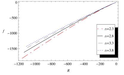
Figure 1: Reconstructed $f(R)$ for NADE with $0\leqslant{z}\leqslant 10$.

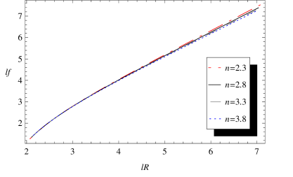
Figure 2: Reconstructed $f(R)$ for NADE in $lf-lR$ plane with $0\leqslant{z}\leqslant 10$.

In [24], the constraint on parameter $n$ is developed from the cosmological data for a flat universe consisting of DE and matter component, the best fit value is found to be $n=2.76^{+0.111}_{-0.109}$. For the non-flat universe, Zhang et al. [25] found that the most appropriate measure of $n$ from the WMAP 7-yr observations is $n=2.673^{+0.053+0.127+0.199}_{-0.077-0.151-0.222}$. In this study, we set $n=2.3,~{}2.8,~{}3.3,~{}3.8$ and $\Omega_{M0}=0.27$. For this choice of parameters, the function $f(R)$ is plotted against $R$ as shown in Figure 1. It is clear that functions appear distinct if $|R|$ (or $z=e^{-x}-1$) is large, while these functions seem to coincide for small $|R|$. The evolution of $f$ shown in Figure 1 is quite similar to that for HDE [20]. We also plot these functions on $lf-lR$ plane as shown in Figure 2, where $lf=\ln(-f)$ and $lR=\ln(-R)$. Our results are consistent with that in [19] and the parameter $n$ is appeared as fundamental element in identifying the nature of NADE.

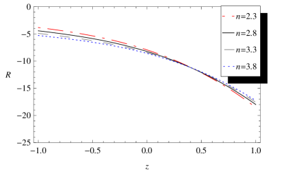
Figure 3: Future evolution of $R$ in NADE with $-1\lesssim{z}\leqslant 1$.

Figure 4: Future evolution of $f(R)$ for $n=2.8$ with $-1\lesssim{z}\leqslant 2$.

To explore the effect of $n$ further, let us see the future evolution of $|R|$. Figure 3 shows that future variation of $|R|$ is alike for different values of $n$ and almost favors the cosmological constant. In Figures 4 and 5, we present the future evolution of $f$ for $n=2.3,~{}2.8,~{}3.3,~{}3.8$. For $n=2.8$, the curve seems to be similar to that for $c=1$ in HDE but in the late stage of the universe there would be a sudden change. The evolution of $f$ is similar for other values of $n$ which is shown in Figure 5. These plots indicate distinct characteristics for the NADE.

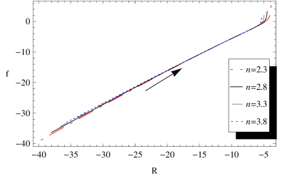
Figure 5: Future evolution of $f(R)$ for different values of $n$ with $-1\lesssim{z}\leqslant 2$.

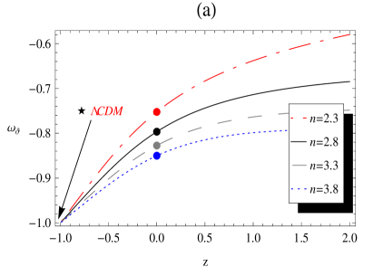
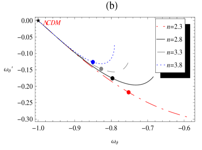
Figure 6: Evolution trajectories in NADE for (a) $\omega_{\vartheta}$ vs $z$ and (b) $\omega_{\vartheta}$ and $\omega_{\vartheta}^{\prime}$ in $\omega_{\vartheta}-\omega_{\vartheta}^{\prime}$ plane with $-1\lesssim{z}\leqslant 2$.

We extend our discussion and explore the evolution of NADE for the cosmographic parameters such as EoS parameter, deceleration parameter, statefinder diagnostic and $\omega_{\vartheta}-\omega^{\prime}_{\vartheta}$ analysis. It is clear from Eq.(6) that NADE does not permit the crossing of phantom divide line $\omega_{\vartheta}=-1$, also if $z\rightarrow-1$ and $\Omega_{\vartheta}\rightarrow 1$ then $\omega_{\vartheta}\rightarrow-1$ in future evolution of NADE. Figure 6(a) shows that for our choice of parameter $n$, the EoS parameter of NADE favors the quintessence era and in the late time, it mimics the cosmological constant regime. We also show the evolution of $\omega_{\vartheta}^{\prime}$ in $\omega_{\vartheta}-\omega_{\vartheta}^{\prime}$ plane for different values of $n$ in NADE. Figure 6(b) depicts that the $\omega_{\vartheta}-\omega_{\vartheta}^{\prime}$ plane represents the $\Lambda$CDM model $(\omega_{\vartheta}=-1,~{}\omega_{\vartheta}^{\prime}=0$) when $z\rightarrow-1$ (or $x\rightarrow{\infty}$). The present values of $\omega_{\vartheta}$ and $\omega_{\vartheta}^{\prime}$ are denoted by dots on each curve. For $n=2.3,~{}2.8,~{}3.3$ and $3.8$, the present values of ($\omega_{\vartheta},~{}\omega_{\vartheta}^{\prime}$) are given by $(-0.752,-.218),~{}(-0.796,-.175),~{}(-0.827,-.147)$ and $(-0.850,-.126)$, respectively.

Sahni et al. [26] defined the statefinder diagnostic parameters $\{r,s\}$ of the form

$$r=\frac{\dddot{a}}{aH^{3}},\quad s=\frac{(r-1)}{3(q-1/2)}.$$ (17)

Introducing the EoS parameter and dimensionless density of DE, Eq.(17) is transformed as

$$r = 1-\frac{3}{2}\Omega_{\vartheta}\left[\omega_{\vartheta}^{\prime}-3\omega_{\vartheta}(1+\omega_{\vartheta})\right],$$ (18)

$$s = \frac{-1}{3\omega_{\vartheta}}\left[\omega_{\vartheta}^{\prime}-3\omega_{\vartheta}(1+\omega_{\vartheta})\right].$$ (19)

The deceleration parameter $q$ in terms of $\omega_{\vartheta}$ and $\Omega_{\vartheta}$ is given by

$$q=\frac{1}{2}(1+3\omega_{\vartheta}\Omega_{\vartheta}).$$ (20)

The variation of deceleration parameter $q$ with $z$ for the NADE without interaction is shown in Figure 7(a). The transition of the universe from decelerating epoch to the accelerated era can be seen and it will end up with $q=-1$ representing the de Sitter model. The sign flip of $q$ depends on the selection of $n$, the era of cosmic acceleration starts earlier for small values of $n$ as compared to larger values.

The plots of statefinder parameters in the $s-r$ plane for $n=2.3,~{}2.8,~{}3.3$ and $3.8$ are shown in Figure 7(b). The dots in the diagram correspond to present day values of statefinder parameters $(r_{0},~{}s_{0})$ which are denoted as $(0.150,0.627)$(red), $(0.129,0.660)$(black), $(0.113,0.691)$(gray) and $(0.100,0.720)$ (blue). The evolution trajectories of the statefinder diagnostic are represented for the future evolution and these will end up to star symbol $\{r=1,s=0\}$, the $\Lambda$CDM model. We also plot the statefinder diagnostic in $q-r$ plane for our selection of parameter $n$ together with the flat $\Lambda$CDM model. It can be seen from Figure 8 that evolution trajectories for NADE in $q-r$ plane commence from the fix point $(q=0.5,~{}r=1)$ which represents the standard cold dark matter regime (SCDM). These curves end at $(q=-1,~{}r=1)$, the de Sitter model in future evolution of the universe. The past and future eras of the universe and present day values of $(q,~{}r)$ are represented by stars and dots, respectively.

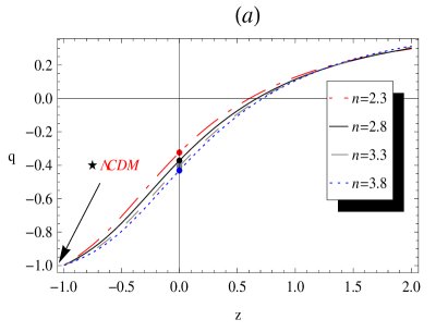
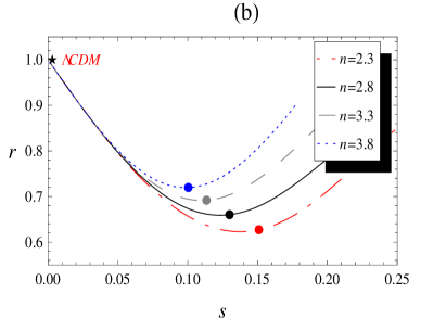
Figure 7: Evolution trajectories in NADE for (a) $q$ vs $z$ and (b) the statefinder diagnostic in $s-r$ plane with $-1\lesssim{z}\leqslant 2$.

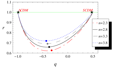
Figure 8: The statefinder plot for NADE in $q-r$ plane. The green line represents the $\Lambda$CDM with $-1\lesssim{z}\leqslant 2$.

3 Reconstruction from NHDE

The energy density of HDE with Granda-Oliveros cutoff is given by [9]

$$\rho_{\vartheta}=3M^{2}_{p}(\mu{H}^{2}+\upsilon\dot{H}),$$ (21)

where $\mu$ and $\upsilon$ are positive constants. Using this value of $\rho_{\vartheta}$, Eq.(4) can be written in the form

$$E^{2}(x)=\frac{2}{2(1-\mu)+3\upsilon}\Omega_{M0}e^{-3x}+g_{0}e^{\frac{2x(1-\mu)}{\upsilon}},$$ (22)

where $E(x)=H(x)/H_{0}$, $H_{0}$ is the present day value of Hubble parameter and $g_{0}$ is the constant of integration which can be obtained using the condition $E(x=0)=1$ as

$$g_{0}=1-\frac{2}{2(1-\mu)+3\upsilon}\Omega_{M0}.$$ (23)

Following [9], the NHDE density is expressed as

$$\rho_{\vartheta}=3H_{0}^{2}\left[\frac{2\mu-3\upsilon}{2(1-\mu)+3\upsilon}\Omega_{M0}e^{-3x}+g_{0}e^{\frac{2x(1-\mu)}{\upsilon}}\right].$$ (24)

The pressure of NHDE can be obtained using this value of $\rho_{\vartheta}$ in the conservation equation of DE

$$p_{\vartheta} = -\rho_{\vartheta}-\frac{1}{3}\frac{d{\rho}_{\vartheta}}{dx}=-3H_{0}^{2}\left(\frac{2(1-\mu)+3\upsilon}{3\upsilon}\right)g_{0}e^{\frac{2x(1-\mu)}{\upsilon}}.$$ (25)

Manipulating Eqs.(24) and (25), the EoS parameter of NHDE turns out to be

$$\omega_{\vartheta}=-\frac{[2(1-\mu)+3\upsilon]^{2}g_{0}e^{\frac{2x(1-\mu)}{\upsilon}}}{3\upsilon(2\mu-3\upsilon)\Omega_{M0}e^{-3x}+[2(1-\mu)+3\upsilon]g_{0}e^{\frac{2x(1-\mu)}{\upsilon}}}.$$ (26)

Proceeding in a similar fashion as in the case of NADE, we obtain

$$\mathcal{D}_{3}(x)\frac{d^{3}f}{dx^{3}}+\mathcal{D}_{2}(x)\frac{d^{2}f}{dx^{2}}+\mathcal{D}_{1}(x)\frac{df}{dx}=-\Omega_{M0}e^{-3x},$$ (27)

where $\mathcal{D}_{i}$ are functions of $E(x)$ and its derivatives, see Appendix (A.2). For the HDE with Granda-Oliveros cutoff, the expression for $H(x)$ is directly useable in numerical computations. If we substitute Eq.(22) and constraint (23) in differential equation (27), then the resulting equation can be solved numerically under the boundary conditions (15) and (16).

In [9], the best fit values of parameters $\mu$ and $\upsilon$ are suggested as $\mu\approx 0.93$ and $\upsilon\approx 0.5$ to keep NHDE consistent with the theory of big-bang nucleosynthesis. Wang and Xu [27] developed the best fit values of parameters $(\mu,\upsilon)$ in both flat and non-flat NHDE models from the current observational data. They found the best fit parameters for the flat model as $\mu=0.8502^{+0.0984+0.1299}_{-0.0875-0.1064}$ and $\upsilon=0.4817^{+0.0842+0.1176}_{-0.0773-0.0955}$. In this study, we select the parameters $(\mu=0.85,\upsilon=0.48)$, $(\mu=0.93,\upsilon=0.56)$ and $(\mu=1,\upsilon=0.63)$. The plot of the function $f(R)$ versus $R$ for NHDE is shown in Figure 9(a). It shows that reconstructed $f(R)$ for NHDE is the same for different values of parameters $(\mu,\upsilon)$. We also plot these results on $\emph{lf}-\emph{lR}$ plane as shown in Figure 9(b). To be more definite about the behavior of $f$, we draw plot on $\emph{lf}-x$ plane presented in Figure 10. This shows that different values of parameters do not affect the shapes of curves unless $x>-0.3$ and aftermath these curves would depict different picture.

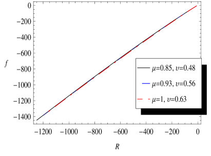
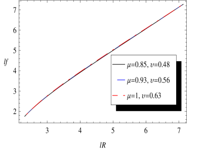
Figure 9: Reconstructed $f(R)$ in (a) $f-R$ plane and (b) $lf-lR$ plane for NHDE with $0\leqslant{z}\leqslant 10$.

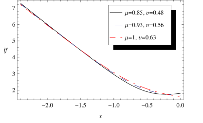
Figure 10: Reconstructed $f(R)$ for NHDE in $lf-x$ plane with $0\leqslant{z}\leqslant 10$, where $x=\ln(1+z)^{-1}$.

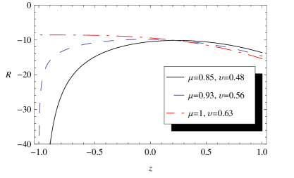
Figure 11: Future evolution of $R$ in NHDE with $-1\leqslant{z}\leqslant 1$.

In order to explore the distinctive effect of parameters $(\mu,\upsilon)$, we get insight of future evolution. First we investigate the future evolution of $R$ versus red shift which is shown in Figure 11. For $(\mu,\upsilon)<(1,0.63)$, $|R|$ would take infinitely large values in future which indicate the phantom era with $\omega_{\vartheta}<-1$ dominating over the matter part, leading to the big rip singularity. When $(\mu,\upsilon)=(1,0.63)$, there is a slight variation in $|R|$ and diagram assures the DE model with $\omega_{\vartheta}=-1$, the cosmological constant.

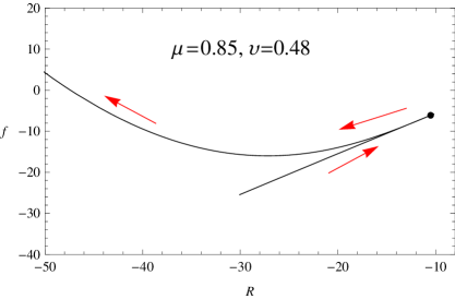
Figure 12: Future evolution of $f(R)$ for $(\mu,\upsilon)=(0.85,0.48)$ with $-1\lesssim{z}\leqslant 2$. The dot denotes the present day and is the point of reversion for DE dominated model.

The difference in the selected parameters $(\mu,\upsilon)$ can be seen more effectively in the future evolution of $f$ reconstructed according to the NHDE as shown in Figures (12)-(14). For $\mu=0.85$ and $\upsilon=0.48$ in Figure 12, the curve shows that initially $|R|$ decreases before reaching the present epoch $(x=0)$ which changes its direction and it would increase leading to the phantom DE. In this scenario, $|R|$ keeps growing whereas $f$ initially decreases and then attains positive value approaching to $+\infty$. In fact, in phantom DE models the point of reversion is a common characteristic because the DE components succeed in their competition with matter contents of the universe. For $\mu=0.93$ and $\upsilon=0.56$, we have almost identical picture as in Figure 12 but here growing rate in $f$ is comparatively large. For $\mu=1$ and $\upsilon=0.63$, we have a linear dependence of $f$ on $R$ leading to constant which is in accordance to the de Sitter model, where $f(R)=R+\Lambda$.

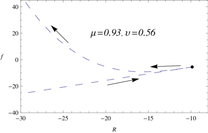
Figure 13: Future evolution of $f(R)$ for $(\mu,\upsilon)=(0.93,0.56)$ with $-1\lesssim{z}\leqslant 2$. The dot denotes the present day and is the point of reversion for DE dominated model.

Figure 14: Future evolution of $f(R)$ for $(\mu,\upsilon)=(1,0.63)$ with $-1\lesssim{z}\leqslant 2$. The dot denotes the present day and is the point of reversion for DE dominated model.

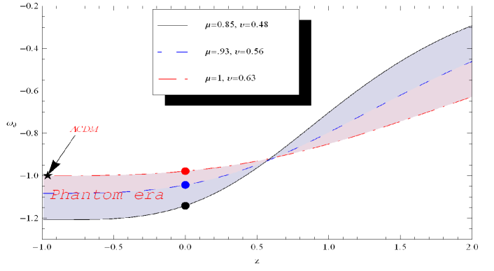
Figure 15: Evolution trajectories of EoS parameter in NHDE for different values of parameters $(\mu,\upsilon)$ with $-1\lesssim{z}\leqslant 2$. The dot denotes the present day and star represents the $\Lambda$CDM model.

Now we discuss the evolution of the NHDE for the selected parameters $(\mu,\upsilon)$ and interpret the behavior of EoS parameter, deceleration parameter and statefinder diagnostic. The plot of EoS parameter for future evolution in NHDE is shown in Figure 15. It shows that the NHDE represents the de Sitter phase of the universe for $(\mu,\upsilon)=(1,0.63)$. For $(\mu,\upsilon)<(1,0.63)$, the EoS parameter intersects the phantom divide line ($\omega_{\vartheta}=-1$) and behaves as quintom model of DE [28]. In this perspective, $\omega_{\vartheta}$ ends up with phantom era which may lead to cosmic doomsday when all the astronomical objects will be ripped apart. It is evident that domain of $\omega_{\vartheta}$ in NHDE is consistent with the observational data of WMAP5 which establishes range of $-1.11<\omega_{\vartheta}<-0.86$ [29].

The evolution of $q$ is represented in Figure 16 which confirms the behavior of $\omega_{\vartheta}$. The curve for $(\mu,\upsilon)=(1,0.63)$ assures the $\Lambda$CDM model with $q=-1$. The transition from deceleration to accelerated epoch can be seen from this plot and the values of redshift at the transition point are consistent with the observational results [30]. The plot of statefinder diagnostic in NHDE for different values of parameters $(\mu,\upsilon)$ is shown in Figure 17. The dot represents the fix point ${r=1,s=0}$ (i.e., the de Sitter phase) and all the curves pass through this point.

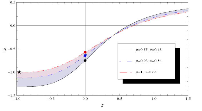
Figure 16: Evolution trajectories of $q$ in NHDE for different values of parameters $(\mu,\upsilon)$ with $-1\lesssim{z}\leqslant 2$. The dot denotes the present day and star represents the $\Lambda$CDM model.

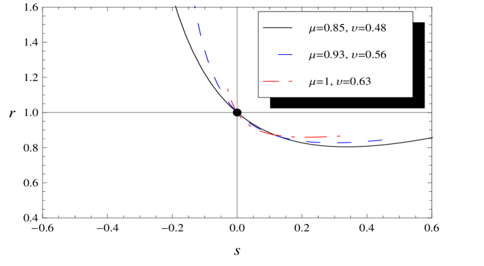
Figure 17: Evolution trajectories of statefinder diagnostic in NHDE for different values of parameters $(\mu,\upsilon)$ with $-1\lesssim{z}\leqslant 2$.

4 Conclusions

The $f(R)$ theory stands as one of the prosperous contexts to describe the cosmic evolution and the present day observational consequences. This theory appears to be a potential candidate in explaining the late time accelerated expansion. A profound model which can explain the cosmic evolution in a definite way is still under consideration. The cosmological reconstruction of $f(R)$ gravity has been explored in [19]-[23] and the issue of which approach should be used is still alive. In refs.[22, 23], $f(R)$ function corresponding to a class of HDE models has been constructed by assuming some ansatz for the scale factor in FRW background. A more effective scheme to reconstruct $f(R)$ theory from the given evolution history $H(z)$ is developed by Capozziello et al. [19]. In this scheme, the significant thing is that we can develop the correspondence of $f(R)$ theory to the given DE model by using the expression of respective $H(z)$. As a result, one can find the $f(R)$ theory which explains the same dynamics (i.e., the cosmic evolution) as predicted by the given DE model. Now it is of interest to consider the modified HDE models and address the intrinsic degeneracy among the $f(R)$ theory and DE models. We find that predictions of both candidates ($f(R)$ theory and DE models) reconcile as they represent distinct features of the same picture.

In this work, we have reconstructed the function $f(R)$ according to NADE and NHDE in flat FRW geometry. The numerical reconstruction scheme is applied to obtain the evolution trajectories of $f$ in different scenarios. In this reconstruction procedure, the Hubble parameter plays a significant role as we transform all quantities in terms of $H$ and $\dot{H}$. We summarize our results as follows:

• For NADE, $H$ is given in terms of $\Omega_{\vartheta}$, so we solve the system of evolution equations for both $\Omega_{\vartheta}$ and $f$. The results are shown in Figures 1 and 2 which are consistent with the constructed functions in literature [19]-[21]. In comparison with HDE, the future variation of $|R|$ and $f$ show identical behavior for different values of $n$. We can say that the behavior of $f$ suggest the de Sitter phase in late time evolution of the universe. The cosmological parameters have been explored in NADE for $n=2.3,2.8,3.3,3.8$ to make sure the evolution of $f$. Figures 5-8 evidently show that NADE favors the quintessence regime and in future evolution, it may end up with the de Sitter phase. Thus our results for reconstructed $f(R)$ are consistent with the independent evolution of NADE. We would like to emphasize that we have taken significantly different values of $n$ but all of these contribute similar results.

• In case of HDE with Granda-Oliveros cutoff, the Hubble parameter in the form $E(x)=H(x)/H_{0}$ is directly used in numerical calculations. We have shown the function $f$ in $f-R$ and $lf-lR$ planes in Figure 9. These curves seem to be identical for different values of parameters $(\mu,\upsilon)$ and slight difference is found for $lf-x$ plane which is shown in Figure 10. Further, we probe the future evolution of $|R|$ and obtain distinct variations accordingly as $(\mu,\upsilon)\leqslant(1,0.63)$. The future evolution of $f$ in Figures 12-14 evidently show the role of parameters $(\mu,\upsilon)$. These plot represent distinct features of $f$ which have been later confirmed by the evolution trajectories of $\omega_{\vartheta}$ and $q$ in Figures 15 and 16. For $(\mu,\upsilon)=(0.85,0.48)~{}\&~{}(0.93,0.56)$, it can be seen that $f$ depicts the phantom DE era and in such case $\omega_{\vartheta}<-1$ and $q<-1$. For $(\mu,\upsilon)=(1,0.63)$, we have $f$ representing the de Sitter phase with $\omega_{\vartheta}=-1$ and $q=-1$. Thus, our results for the function $f$ corresponding to NHDE coincide with that of cosmographic parameters.

It is to be noted that NADE and NHDE models are developed in the context of general relativity rather than any modified theory such as $f(R)$ gravity. We have reconstructed $f(R)$ by considering the curvature part as an effective description of these DE models. We also emphasize that this work is more comprehensive when comparing with previous ones as it involves the analysis of cosmological parameters to ensure the evolution of reconstructed function $f(R)$.

Acknowledgment

We would like to thank the Higher Education Commission, Islamabad, Pakistan for its financial support through the Indigenous Ph.D. 5000 Fellowship Program Batch-VII.

Appendix A

$$\mathcal{B}1 = 2H^{2}\left(\frac{d^{2}R}{dx^{2}}\right)\left(\frac{d^{2}R}{dx^{2}}\right)^{-3}-\left[H^{2}\frac{d^{3}R}{dx^{3}}+\left(\frac{1}{2}\frac{dH^{2}}{dx}-H^{2}\right)\frac{d^{2}R}{dx^{2}}\right]\left(\frac{dR}{dx}\right)^{-2}$$

$$+ \frac{dH^{2}}{dx}\left(\frac{dR}{dx}\right)^{-1},$$

$$\mathcal{B}2 = -2H^{2}\left(\frac{d^{2}R}{dx^{2}}\right)\left(\frac{dR}{dx}\right)^{-2}+\left(\frac{1}{2}\frac{dH^{2}}{dx}-H^{2}\right)\left(\frac{dR}{dx}\right)^{-1},$$

$$\mathcal{B}3 = H^{2}\left(\frac{dR}{dx}\right)^{-1},$$ (A.1)

$$\mathcal{D}1 = 2E^{2}\left(\frac{d^{2}R}{dx^{2}}\right)\left(\frac{d^{2}R}{dx^{2}}\right)^{-3}-\left[E^{2}\frac{d^{3}R}{dx^{3}}+\left(\frac{1}{2}\frac{dE^{2}}{dx}-E^{2}\right)\frac{d^{2}R}{dx^{2}}\right]\left(\frac{dR}{dx}\right)^{-2}$$

$$+ \frac{dE^{2}}{dx}\left(\frac{dR}{dx}\right)^{-1},$$

$$\mathcal{D}2 = -2E^{2}\left(\frac{d^{2}R}{dx^{2}}\right)\left(\frac{dR}{dx}\right)^{-2}+\left(\frac{1}{2}\frac{dE^{2}}{dx}-E^{2}\right)\left(\frac{dR}{dx}\right)^{-1},$$

$$\mathcal{D}3 = E^{2}\left(\frac{dR}{dx}\right)^{-1}.$$ (A.2)

References

- [1] Perlmutter, S. et al.: Astrophys. J. 517(1999)565; Spergel, D.N. et al.: Astrophys. J. Suppl. 148(2003)175; Tegmark, M. et al.: Phys. Rev. D 69(2004)103501; Riess, A.G. et al.: Astrophys. J. 659(2007)98; Fedeli, C., Moscardini, L. and Bartelmann, M.: Astron. Astrophys. 500(2009)667.
- [2] Cohen, A.G., Kaplan, D.B. and Nelson, A.E.: Phys. Rev. Lett. 82(1999)4971.
- [3] Li, M.: Phys. Lett. B 603(2004)1.
- [4] Hsu, S.D.H.: Phys. Lett. B 594(2004)13.
- [5] Wei, H. and Cai, R.-G.: Phys. Lett. B 660(2008)113.
- [6] Wu, J.-P., Ma, D.-Z. and Ling, Y.: Phys. Lett. B 663(2008)152.
- [7] Liu, X.-L. and Zhang, X.: Commun. Theor. Phys. 52(2009)761.
- [8] Jamil, M. and Saridakis, E.N.: JCAP 07(2011)028.
- [9] Granda, L.N. and Oliveros, A.: Phys. Lett. B 669(2008)275; ibid. 671(2009)199.
- [10] Sharif, M. and Jawad, A.: Eur. Phys. J. C 72(2012)2097.
- [11] Sotiriou, T.P and Faraoni, V.: Rev. Mod. Phys. 82(2010)451; De Felice, A. and Tsujikawa, S.: Living Rev. Rel. 13(2010)3; Sharif, M. and Zubair, M.: Astrophys. Space Sci. 342(2012)511; Bamba, K. Capozziello, S. Nojiri, S. and Odintsov, S.D.: Astrophys. Space Sci. 345(2012)155.
- [12] Harko, T., Lobo, F.S.N., Nojiri, S. and Odintsov, S.D.: Phys. Rev. D 84(2011)024020.
- [13] Sharif, M. and Zubair, M.: JCAP 03(2012)028; ibid. Erratum: 05(2012)E01.
- [14] Sharif, M. and Zubair, M.: J. Phys. Soc. Jpn. 81(2012)114005.
- [15] Sharif, M. and Zubair, M.: J. Phys. Soc. Jpn. 82(2013)014002.
- [16] Sharif, M. and Zubair, M.: Cosmology of Holographic and New Agegraphic Models, J. Phys. Society of Jpn. (to appear, 2013).
- [17] Sharif, M. and Zubair, M.: Thermodynamic Behavior of Particular Gravity Models, J. Exp. Theor. Phys. (to appear, 2013).
- [18] Cognola, G., Elizalde, E., Nojiri, S., Odintsov, S.D. and S. Zerbini: Phys. Rev. D 73(2006)084007; Sharif, M. and Abbas, G.: J. Phys. Soc. Jpn. 82(2013)034006.
- [19] Capozziello, S. Cardone, V.F. and Troisi, A.: Phys. Rev. D 71(2005)043503.
- [20] Wu, X. and Zhu, Z.-H.: Phys. Lett. B 660(2008)293.
- [21] Feng, C.-J.: Phys. Lett. B 676(2009)168.
- [22] Setare, M.R.: Int. J. Mod. Phys. D 17(2008)2219; Astrophys. Space Sci. 326(2010)27.
- [23] Karami, K. and Khaledian, M.S.: JHEP 03(2011)086.
- [24] Wei, H. and Cai, R.-G.: Phys. Lett. B 663(2008)1.
- [25] Zhang, J.-F., Li, Y.-H. and Zhang, X.: Eur. Phys. J. C 73(2013)2280.
- [26] Sahni, V., Saini, T.D., Starobinsky, A.A. and Alam, U.: JETP Lett. 77(2003)201; Pisma Zh. Eksp. Teor. Fiz. 77(2003)249.
- [27] Wang, Y. and Xu, L.: Phys. Rev. D 81(2010)083523.
- [28] Wei, H., Cai, R. G. and Zeng, D. F.: Class. Quantum Grav. 22(2005)3189.
- [29] Komatsu, E. et al.: Astrophys. J. Suppl. 180(2009)330.
- [30] Ma, Y.-Z.: Nucl. Phys. B 804(2008)262; Daly, R. A. et al.: The Astrophysical Journal 677(2008)1.