SurvRegCensCov: Weibull Regression for a Right-Censored Endpoint with a Censored Covariate

Stanislas Hubeaux, Kaspar Rufibach SurvRegCensCov: Weibull Regression for a Right-Censored Endpoint with a Censored Covariate SurvRegCensCov: Weibull Regression with a Censored Covariate Biomarker data is often subject to limits of quantification and/or limits of detection. Statistically, this corresponds to left- or interval-censoring. To be able to associate a censored time-to-event endpoint to a biomarker covariate, the R package SurvRegCensCov provides software for Weibull regression for a right-censored endpoint, one interval-censored, and an arbitrary number of non-censored covariates. Furthermore, the package provides functions to estimate canonical parameters from censored samples based on several distributional assumptions, and a function to switch between different parametrizations used in R for Weibull regression. We illustrate the new software by applying it to assess Prentice’s criteria for surrogacy in data simulated from a randomized clinical registration trial. Weibull Regression, censored covariate, limit of detection, biomarker, surrogacy, Prentice’s criteria, R Weibull Regression, censored covariate, limit of detection, biomarker, surrogacy, Prentice’s criteria, R Stanislas Hubeaux
École polytechnique fédérale de Lausanne
E-mail:

Kaspar Rufibach
F. Hoffmann-La Roche AG
Building 670, Room 517
4070 Basel, Switzerland
Telephone: +41/0/61687-5341
E-mail:
URL: http://www.roche.com

1 Introduction

In survival analysis, we typically seek to analyze the association between a collection of covariates and a time-to-event endpoint. Regression models, such as Cox or parametric regression, are well-developped and available for the common situation where the endpoint is right- or even interval-censored, see e.g.,, Klein and Moeschberger (2003). However, when analyzing biomarkers it may happen that also one or more covariates are censored, typically left-censored at a limit of detection (LOD) $c$ which is given by assay sensitivity, i.e., the researcher only knows that the actual value of a biomarker, say, is $\leq c$, but does not know the exact measurement. We refer to Arunajadai and Rauh (2012) and Bernhardt et al. (2014) for overviews on methods how to handle left-censored data, to Langohr et al. (2004) for the description of a parametric survival regression model with a censored discrete covariate, and to Armbruster and Pry (2008) for a discussion of the different types of limits that appear in generation of biomarker data.

Bernhardt et al. (2014) also provides a discussion of “traditional” approaches to treat left-censoring in covariates, namely complete case analysis or various imputation methods, e.g., replacing a left-censored observation by the limit of detection $c$ itself, by $c/2$, or $c/\sqrt{2}$. As long as the censoring does not depend on the survival time, removing observations below $c$ still yields consistent estimates, however, at the cost of reduced efficiency (Bernhardt et al., 2014, Proposition 1). Arunajadai and Rauh (2012) show that naïve implementation methods typically yield potentially hugely biased estimates and they recommend that, since there are no specific sets of conditions under which imputation methods can be guaranteed to perform well, these methods should generally not be used. In addition to their empirical inferiority, there is also not much theoretical justification for these naïve approaches. $c/2$ could be seen as taking the mean of a Uniform random variable on $[0,c]$, but the motivation of $c/\sqrt{2}$ is not clear.

To correctly account for the nature of the data, i.e., censored time-to-event endpoint with a left-censored covariate, Sattar et al. (2012) derive and maximize a likelihood function assuming a Weibull distribution for the time-to-event endpoint and one left-censored covariate. To be able to incorporate the latter in a fully parametric survival regression model, a fully-known distribution for the left-censored covariate has to be imposed. In Sattar et al. (2012), a Normal distribution is assumed for the left-censored covariate. As we are in a fully parametric model, statistical inference can be based on standard likelihood theory. So far, no publicly available software is available that provides estimates and inference in this model. SurvRegCensCov closes this gap. Our implementation extends the work of Sattar et al. (2012) with respect to the following features:

• We allow for estimation of the shape parameter $\gamma$ of the Weibull distribution, which was set to 1 in the simulations in Sattar et al. (2012).

• As we outline in our example in Section 4, in applications the incompletely observed covariate sometimes is not only left- but rather interval-censored. Our implementation allows for that data structure.

• In the example we use for illustration, the regression model involves at least one more non-censored covariate in addition to the censored covariate. We thus extend the code described in Sattar et al. (2012) to be able to take into account an arbitrary number of non-censored covariates. As a matter of fact, no non-censored covariate, i.e., a Weibull regression model involving only the censored covariate, can also be handled using SurvRegCensCov.

• The likelihood function set up to accommodate the Weibull regression model necessitates for every censored covariate observation computation of a rather involved integral, see Section 3. Sattar et al. (2012) suggest to use Simpson’s 1/3 rule for computation of these integrals, implying (if we understand their approach correctly) that certain tuning parameters have to be selected. We proceed differently and omit this choice of tuning parameters, see Section 3.

• Finally, we provide some functions to easily switch between different parametrizations used for Weibull regression models.

1.1 About this document

The package is available from the Comprehensive R Archive Network at http://CRAN.R-project.org/package=SurvRegCensCov (R Core Team, 2014).

This document was created using Sweave (Leisch, 2002), LaTeX (Knuth, 1984; Lamport, 1994), and R (R Core Team, 2014). This means that all of the code has been checked by R.

2 Methods

2.1 Two-sample inference for censored Normal samples

Lynn (2001) describes maximum likelihood estimation for one left-censored sample based on parametric assumptions. proc lifereg in SAS and the R package fitdistrplus (Delignette-Muller et al., 2013) implement that methodology for a large catalogue of distributions to choose from. proc lifereg also allows for inference based on two samples, for a variety of distributions. In the Normal case proc lifereg implicitly assumes that the variances in the two groups are identical. However, in our applications we typically do not want to entertain that restriction, and that is why we have added the function NormalMeanDiffCens to SurvRegCensCov. It allows for inference from two independent interval-censored samples assumed to come from Normal distributions with different means and variances. Note that the default setting for the t.test function, i.e., inference from two completely observed Normal samples, is indeed as well var.equal = FALSE. We illustrate the application of NormalMeanDiffCens in Section 4.

In addition to a function for the two-sample Normal case, SurvRegCensCov also provides a function (ParamSampleCens) to estimate canonical parameters from one sample, for the Normal, Logistic, Gamma, and Weibull distribution. Note that the function fitdistcens in the package fitdistrplus (Delignette-Muller et al., 2013) offers similar functionality.

2.2 Weibull regression model with a censored covariate - the model

Define a triple $(T,\delta,\mathbf{X})$, where $T$ denotes the follow-up time, $\delta$ is the censoring indicator, and $\mathbf{X}\in\mathbb{R}^{d}$ is a (time-invariant) vector of baseline covariates. The actual survival time is $Z$ and the censoring time $C$, so that we observe $T=\min\{Z,C\}$ and $\delta=1\{T\leq Z\}$, with $1\{\cdot\}$ the indicator function. The survival time $Z$ is assumed to be conditionally independent given $\mathbf{X}$, i.e., the censoring is supposed to be non-informative. Sattar et al. (2012) then assume that $Z$ follows a Weibull distribution with shape parameter $\gamma$ and scale parameter $\lambda$, so that the density and hazard function of $Z$ are defined as

$$f_{0}(z)\ =\ \lambda\gamma z^{\gamma-1}\exp(-\lambda z^{\gamma}) h_{0}(z)\ =\ \lambda\gamma z^{\gamma-1}.$$ (1)

This is the parametrization used by Klein and Moeschberger (2003, Chapter 12). Note that R’s dweibull function uses another parametrization, namely

$$f^{*}_{0}(z)\ =\ (a/b)(z/b)^{a-1}\exp\Bigl{(}-(z/b)^{a}\Bigr{)} h^{*}_{0}(z)\ =\ (a/b)(z/b)^{a-1},$$

so that the reparametrization is $\gamma=a,\lambda=b^{-a}$. Yet another parametrization is used by the survreg function in survival (Therneau, 2013; Therneau and Grambsch, 2000), see (2).

Using Parametrization (1) to set up a Weibull regression, we then assume that the hazard function, for a given covariate vector $\mathbf{X}$ and a corresponding vector $\mathbf{\beta}$ of regression parameters, can be written as

$$h(z|\mathbf{X}) = \exp(\mathbf{\beta}^{\top}\mathbf{X})h_{0}(z)$$

$$= \exp(\mathbf{\beta}^{\top}\mathbf{X})\lambda\gamma z^{\gamma-1}$$

$$=: \lambda^{\star}\gamma z^{\gamma-1}.$$

The last equality shows that we model the scale parameter $\lambda^{\star}=\lambda\exp(\mathbf{\beta}^{\top}\mathbf{X})$ using a base scale $\lambda$ and covariates. The coefficients $\exp\mathbf{\beta}$ feature the proportional hazards property, i.e., can be interpreted as hazard ratios. On the other hand, survreg embeds Weibull regression in the framework of a more general accelerated failure time model and its output provides estimates for $\log(\sigma)$ (denoted Log(scale)), $-\mu/\sigma$ (Intercept), and the regression parameters $\alpha$. The reparametrization from (1) is

$$\gamma\ =\ \sigma^{-1},\ \ \lambda\ =\ \exp(-\mu/\sigma),\ \ \mathbf{\beta}\ =\ -\alpha/\sigma.$$ (2)

In SurvRegCensCov, the function ConvertWeibull takes the output of survreg as input and transforms parameter estimates to Parametrization (1), thereby allowing to easily switch from the accelerated failure time to the proportional hazard interpretation. Transformed confidence intervals, based on applying the $\delta$-rule to survreg’s standard errors (see Klein and Moeschberger, 2003, Section 12.2), are available as well. ConvertWeibull also computes the “acceleration factor” $\exp\mathbf{\alpha}$, alternatively called “event time ratio”, see e.g., Carroll (2003) for how to interpret it. Note that the Weibull distribution is the only parametric family that allows to set up a regression model that allows for both, a proportional hazard and an accelerated failure time interpretation.

2.3 Maximum likelihood estimation of parameters

Now assume we have an i.i.d. sample $(T_{i},\delta_{i},\mathbf{X}_{i}),i=1,\ldots,n$ of observations and want to estimate the parameter vector $(\gamma,\lambda,\mathbf{\beta})$ based on this data and maximum likelihood. The corresponding likelihood function for completely observed $\mathbf{X}_{i}$ is, according to Sattar et al. (2012),

$$L_{1}(\gamma,\lambda,\mathbf{\beta}) = \prod_{i=1}^{n}h(T_{i}|\mathbf{X})^{\delta_{i}}S(T_{i}|\mathbf{X})$$

$$= \prod_{i=1}^{n}f(T_{i}|\mathbf{X})^{\delta_{i}}S(T_{i}|\mathbf{X})^{1-\delta_{i}}.$$

For the moment, let us further assume that we observe some of the entries of the first covariate $(X_{11},\ldots,X_{1n})$ only if it is above the patient-specific LOD $c_{i}$ and that for those values below $c_{i}$, we simply use some imputation scheme, typically just impute $c_{i}$. Then, maximum likelihood estimates (MLE) based on $L_{1}$ are in general biased (D’Angelo and Weissfeld, 2008; Sattar et al., 2012). In order to account for $X_{1i}$ potentially being censored, Sattar et al. (2012) make additional assumptions and modify the likelihood function as follows: First, we explicitly specify a distribution for $X_{1i}$ by specifying the density $f_{\theta}$, where $\theta\in\mathbb{R}^{d}$ indicates the parametrization of $f$, for $d\geq 1$. Note that they assume the same distribution for all observations. Often, it seems sensible to assume $f_{\theta}=f_{\mu,\sigma^{2}}$ as Normal, maybe after taking the logarithm of $X_{1i}$. Define for each observation the binary random variable $R_{i}:=1\{X_{1i}\geq c_{i}\}$ that indicates the status of the observation, i.e., whether it is observed or left-censored. The probability mass function $p_{R_{i}}$ of $R_{i}$ is a simple Bernoulli distribution with success probability $\pi_{i}=P(X_{1i}>c_{i})=\int_{c_{i}}^{\infty}f_{\theta}(x)dx$ that $X_{1i}$ is observed.

Klein and Moeschberger (2003, Chapter 3.5) explain how arbitrarily censored data contributes to the likelihood function when we estimate parameters from a random sample. Sattar et al. (2012, Formula 2) use this to construct the Weibull regression likelihood function based on our available data including a left-censored covariate, yielding

$$L_{2}(\gamma,\lambda,\mathbf{\beta}) = \prod_{i=1}^{n}\Bigl{(}f(T_{i}|\mathbf{X})^{\delta_{i}}S(T_{i}|\mathbf{X})^{1-\delta_{i}}p_{R_{i}}(r_{i})f_{\theta}(X_{1i})\Bigr{)}^{r_{i}}\times$$

$$\hskip 14.22636pt\Bigl{(}\int_{-\infty}^{c_{i}}f(T_{i}|\mathbf{X})^{\delta_{i}}S(T_{i}|\mathbf{X})^{1-\delta_{i}}p_{R_{i}}(r_{i})f_{\theta}(x)dx\Bigr{)}^{1-r_{i}}.$$

This likelihood can in general not be written in closed form and has thus to be maximized numerically. The MLE is defined as

$$(\widehat{\gamma},\widehat{\lambda},\mathbf{\widehat{\beta}}) := \mathop{\rm arg\,max}_{(\gamma,\lambda,\mathbf{\beta})\in\mathbb{R}^{2+d}}\log L_{2}(\gamma,\lambda,\mathbf{\beta}).$$

Extension to interval-censoring and more than one censored covariate is straightforward, but tedious. The function SurvRegCov in SurvRegCensCov provides standard errors of the estimates $(\widehat{\gamma},\widehat{\lambda},\mathbf{\widehat{\beta}})$ based on the observed Fisher information matrix.

3 Implementation

To maximize $L_{2}$, we use R’s function optim. Note that maximization of $L_{2}$ is not entirely straightforward, as for each evaluation of $L_{2}$ at a given value of the parameter vector $(\gamma,\lambda,\mathbf{\beta})$, $n-\sum_{i=1}^{n}R_{i}$ integrals have to be numerically computed. As discussed in Section 1, Sattar et al. (2012) use an approximation rule to compute the integrals, and - if we interpret their description of implementation correctly - their approach necessitates the choice of the tuning parameters $a,b,h$, where $[a,b]$ is the interval the function to be integrated “lives on” and $h$ is the grid length. In our initial implementation of Sattar et al. (2012)’s approach, the choice of these parameters might depend on the actual data, i.e., the maximization of the log-likelihood function potentially needs to be tuned manually for a given dataset. Instead, we simply set very small values of the function to be integrated to 0. We can then use R’s integrate function to do the repeated integrations, implying a considerable gain in computational speed without sacrifying numerical accuracy of the resulting estimates. The modification also implies that the maximization of the log-likelihood function in our SurvRegCensCov is fully automatic and does not necessitate the choice of tuning parameters.

To compute the Hessian matrix of the log-likelihood function we use the package numDeriv (Gilbert and Varadhan, 2012). The latter generally provides more accurate computations of derivatives in complex problems than optim.

The function SurvRegCens in SurvRegCensCov implements maximization of $L_{2}$, and provides standard statistical inference for the resulting parameter estimate $(\widehat{\gamma},\widehat{\lambda},\mathbf{\widehat{\beta}})$. In addition to this main function of the package, SurvRegCensCov provides ConvertWeibull to reparametrize the output of survreg, WeibullReg does these two steps in one function, and WeibullDiag constructs a diagnostic plot to visually check the adequacy of the Weibull distribution for survival data with respect to one nominal covariate.

4 Examples

Sattar et al. (2012) illustrate Weibull regression with a left-censored covariate and no completely observed covariate using the Genetic and Inflammatory Marker of Sepsis (GenIMS) study (Yende et al., 2008). The interest was to associate the right-censored endpoint to some cytokine levels which were subject to a uniform LOD $c$.

4.1 Surrogacy

Our incentive to implement the methodology came from another application: So far, registrational studies for new drugs in chronic lymphoid leukemia (CLL) typically used progression-free survival (PFS) as their primary endpoint. With the advent of ever more potent therapies in this disease and luckily for patients, PFS is getting longer and longer, especially in those patients that are considered “fit” for aggressive chemotherapy. As an example, the patients in the treatment arm of the CLL8 study (Hallek et al., 2010), a randomized trial in first-line CLL patients, were seen with a median PFS of 57 months (Fisher et al., 2012). As this improvement in PFS continues, clinical studies with PFS as an endpoint become infeasible and surrogate endpoints for PFS are sought. In addition, several treatment regimens are entering the CLL landscape which tackle the disease from different angels and are or will be approved in the near future. In order to establish efficacy of these new therapies, or even combinations between them, “early” measurable endpoints that replace the ever growing PFS are needed. Such a potential early measurable and surrogacy candidate is minimal residual disease (MRD, Bottcher et al., 2012), a continuous endpoint that basically counts the number of cancerous cells left in the body after therapy. MRD can be measured either by IGH polymerase chain reaction (PCR) or flow cytometry. The latter method was used in CLL8 and exhibited a sensitivity of $c:=10^{-4}$, i.e., some of the measurements are indeed left-censored at $c$.

Note that MRD is not a biomarker in the strict sense, but rather an endpoint that measures effect of therapy after patient has undergone treatment. However, left-censoring often occurs when analyzing biomarker data, so that our new software is applicable in a much broader sense than to assess surrogacy only.

The CLL11 study (Goede et al., 2014) established superiority of a 2${}^{\text{nd}}$ generation CD20 antibody, obinutuzumab, over rituximab, a 1${}^{\text{st}}$ generation antibody. In this trial, MRD was measured using PCR via a patient-specific assay. Furthermore, as is typical for small MRD values, the exact value can often not be measured, so that the labs provided a lower and upper limit of detection in these cases, i.e., some of the measurements were in fact genuinely interval-censored. As a consequence, in order to establish surrogacy based on CLL11 data, we indeed needed to extend the setup in Sattar et al. (2012) to allow for interval-censored data.

To formally establish surrogacy, the first step is typically to assess what is called “Prentice’s criteria” (Prentice, 1989). The goal is to show that the hazard for PFS is independent of treatment, conditional on the surrogate variable MRD. In order to do so, a regression model with PFS as endpoint and MRD as well as treatment as covariates has to be set up. Prentice’s criteria can be considered met if in such a model, MRD is associated with the endpoint and captures all the effect of the treatment, i.e., the latter is not anymore associated to the endpoint. Thus, Prentice’s criteria is typically regarded as fulfilled if treatment is not significant anymore at a pre-specififed significance level in this regression model and has a small effect estimate.

In Bottcher et al. (2012), MRD was discretized in three categories using cutoffs $10^{-4}$ and $10^{-2}$. Discretization might make sense clinically, but from a statistical point of view it is well-known that by discretization we loose up to 1/3 of the information in a given continuous variable (Lagakos, 1988). So one of our goals with implementing SurvRegCensCov was to assess Prentice’s criteria for the CLL11 study using the full MRD information, i.e., considering the latter a continuous - but interval-censored - covariate in a Weibull regression model.

4.2 Imitating the CLL11 study

Goede et al. (2014) is the first paper on CLL11 that reports clinical results and only contains very high-level MRD results. No detailed analysis of MRD in CLL11 has been published yet and we are thus not able to illustrate SurvRegCensCov using original CLL11 data, although this study actually initiated our work and motivated the extensions discussed above.

To understand the features of our new and two potential traditional approaches in the context of CLL11, we instead simulate data with similar properties than the one in the rituximab (R, $n=226$) and obinutuzumab (O, $n=221$) treatment arms in CLL11 to illustrate SurvRegCensCov. To this end, we first explored the MRD data. As is typical for biomarker data, original MRD measurements were right-skewed, so that we used $\log$(MRD) in our model. The transformed measurements nicely followed a Normal distribution. Since $\log$(MRD) is a continuous interval-censored variable, we used ParamSampleCens to estimate $\mu$ and $\sigma$ of the assumed Normal distribution, in each treatment arm separately. Applying the function SurvRegCens we finally estimated the canonical parameters $\lambda,\gamma$ and the regression coefficients $\beta_{\text{tmt}}$, $\beta_{\text{MRD}}$ corresponding to treatment and $\log$(MRD) in our Weibull regression model. We end up with eight estimated parameters $\widehat{\mu}_{\text{R}},\widehat{\sigma}_{\text{R}},\widehat{\mu}_{\text{O}},\widehat{\sigma}_{\text{O}},\widehat{\lambda},\widehat{\gamma},\widehat{\beta}_{\text{tmt}}$ and $\widehat{\beta}_{\text{MRD}}$ based on CLL11 data. In addition, we also determined the proportion of censored MRD observations in each treatment arm. Using these estimated parameters and the assumptions of Normality of the density $f_{\theta}$ of the censored covariate and Weibull distributed PFS times, we can simulate right-censored PFS times. Contrasting these simulated PFS times to the original CLL11 data, we get strikingly similar Kaplan-Meier estimates.

To mimick CLL11 data (which we are not able to show at this point) in a small simulation study, we thus sufficiently varied the eight parameters above that define our model, so that no conclusion on the true nature of CLL11 data is possible. Specifically, we assumed $\mu_{\text{R}}=-1.5,\sigma_{\text{R}}=1.5,\mu_{\text{O}}=-3.5,\sigma_{\text{O}}=1.5,\lambda=0.75,\gamma=3.1,\beta_{\text{tmt}}=0$ and $\beta_{\text{MRD}}=0.7$ as well as proportions of 0.05 and 0.35 of left-censored MRD values as well as a sample size of $n=200$ in each simulated arm. We note that the higher proportion of left-censored MRD values in the obinutuzumab arm is indicative of the higher efficacy of that treatment. We deliberately choose the model to have no treatment effect, as this corresponds to the “ideal” situation when indeed MRD is a complete surrogate for PFS. Since in our simulation study we compare Weibull regression with a censored covariate to Weibull and Cox regression where we impute the censored observations by the LOD, we only left-censor MRD in our simulation. This implies that we can compare the newly implemented to the latter more standard methods with imputation at the LOD. MRD values were left-censored at the quantiles corresponding to the empirical censoring proportions $0.05$ and $0.35$ in CLL11.

To illustrate SurvRegCens the chunk below provides its model output received from estimating the model based on the first simulated sample and Figure 1 provides the Kaplan-Meier estimates of this simulated sample:

R> WRmod1 <- SurvRegCens(formula = formula(Surv(time, event)   + Surv(time = mrd.low, time2 = mrd.up, type = "interval2") + + tmt.df), data = data.frame(time, event, mrd.low, mrd.up, + tmt.df), Density = DensityCens, initial = initial, + namCens = "mrd", trace = 0) R> summary(WRmod1) Weibull regression for a right-censored response with an interval-censored covariate

Call: SurvRegCens(formula = formula(Surv(time, event)   Surv(time = mrd.low, time2 = mrd.up, type = "interval2") + tmt), data = data.frame(time, event, mrd.low, mrd.up, tmt), Density = DensityCens, initial = initial, namCens = "mrd", trace = 0)

Coefficients: Estimate Std. Error CI.low CI.up p-value lambda 0.74595 0.08455 0.58024 0.91166 NA gamma 2.98008 0.16942 2.64802 3.31213 NA tmt 0.14092 0.16852 -0.18937 0.47121 0.403 mrd 0.67344 0.06010 0.55565 0.79122 <2e-16

AIC: 2290.1

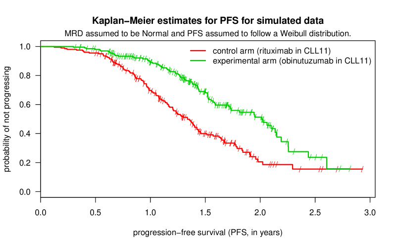
Figure 1: Kaplan-Meier estimates of PFS for first simulated sample.

The model is well able to estimate the parameters of interest and the estimated coefficient of treatment is indeed close to 0, or the hazard ratio exp(Estimator) close to 1, and non-significant at $\alpha=0.05$. The MRD covariate is specified as interval-censored using the coding for type = interval2 in Surv (Therneau, 2013):

R> head(data.frame(mrd.low, mrd.up)) mrd.low mrd.up 1 -1.5124 -1.5124 2 -0.7509 -0.7509 3 -1.7824 -1.7824 4 -1.9962 -1.9962 5 -2.6862 -2.6862 6 NA -3.9673

The estimated parameters of $\log$(MRD) in each treatment arm are R> NormalMeanDiffCens(censdata1 = mrd.r, censdata2 = mrd.o) Estimator Std. Error CI.low CI.up p-value mu1 -1.532 0.10429 -1.737 -1.328 <2e-16 mu2 -3.358 0.10007 -3.554 -3.162 <2e-16 sigma1 1.468 0.07707 1.317 1.619 1.2e-09 sigma2 1.329 0.08474 1.163 1.496 1e-04 Mean difference delta 1.826 0.14454 1.542 2.109 <2e-16

Again, the underlying true parameters are accurately estimated. However, note that in our model in Section 2.3 we assume the same density $f_{\theta}$ for the censored covariate for all observations, so that to estimate WRmod1 above we used DensityCens defined according to R> res1 <- ParamSampleCens(censdata = rbind(mrd.r, mrd.o), dist = "normal") R> res1$coeff\Soutput EstimatorStd.ErrorCI.lowCI.upp-valueMu-2.4670.08774-2.639-2.295<2e-16Sigma1.7120.069751.5761.849<2e-16\Sinput R>DensityCens<-function(value,res=res1){return(dnorm(value,+mean=res$coeff[1,1],sd=res$coeff[2,1]))}\par$

4.3 Simulation results

We generated $M=1000$ “CLL11 like” trials using the parameters above and for each simulation we estimated three regression models for PFS and explanatory variables treatment and $\log$(MRD):

• Weibull regression using the function survreg in survival, where left-censored MRD values were considered to be actual measurements, i.e., we impute the lower limit of detection as an actual MRD value.

• Cox regression with the same imputation strategy, using the function coxph in survival.

• Weibull regression assuming normally distributed $\log$(MRD), correctly accounting for the censoring of MRD via the function SurvRegCensCov.

As discussed in Section 1, imputing the limit of detection for left-censord values is common in applications. Figure 2 provides boxplots of the $1000$ estimated parameters whereas Table 1 displays the bias of each method in estimating the Weibull and/or regression parameters.

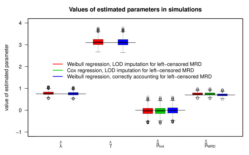
Figure 2: Boxplots of estimated parameters in 1000 simulations.

	$\widehat{\lambda}$	$\widehat{\gamma}$	$\widehat{\beta}_{\text{tmt}}$	$\widehat{\beta}_{\text{MRD}}$
True parameter value we simulated from	0.75	3.1	0	0.7
Bias Weibull regression, correctly accounting for left-censored MRD	0.0069	0.0231	-0.0060	0.0046
Bias Weibull regression, LOD imputation for left-censored MRD	4.7	5.6	4.8	8.5
Bias Cox regression, LOD imputation for left-censored MRD			1.3	10.3

Table 1: Bias for Weibull regression with censored covariate and relative bias for imputation methods. Rows 2 and 3 are factors by which Row 1 is multiplied to get the bias of the other methods. Biases for $\widehat{\beta}_{\text{tmt}}$ were negative for all three methods.

We find that absolute bias is moderate for all three methods, but that clearly Weibull regression correctly accounting for the left-censoring of MRD performs best. This remains true when we look at the mean-squared error in Table 2. Finally, in an analysis of surrogacy we are interested in testing the null hypothesis of no treatment effect in a hypothesis test. As we simulated assuming that $\beta_{\text{tmt}}=0$, by counting how often in our simulations a test for this hypothesis at a significance level of $\alpha=0.05$ rejects we get an empirical assessment how well each method keeps the probability of a type I error. Weibull regression correctly accounting for left-censoring yielded a proportion of 0.05 rejected null hypothesis for the treatment regression parameter, Weibull regression with LOD imputation 0.062, and Cox regression with LOD imputation 0.059. Thus the maximum likelihood estimate exactly keeps the probability of a type I error, whereas the two approximate methods slightly inflate it.

	$\widehat{\lambda}$	$\widehat{\gamma}$	$\widehat{\beta}_{\text{tmt}}$	$\widehat{\beta}_{\text{MRD}}$
True parameter value we simulated from	0.75	3.1	0	0.7
MSE Weibull regression, correctly accounting for left-censored MRD	0.00005	0.00053	0.00004	0.00002
MSE Weibull regression, LOD imputation for left-censored MRD	21.9	31.4	22.8	72.7
MSE Cox regression, LOD imputation for left-censored MRD			1.8	105.9

Table 2: Mean-squared error for Weibull regression with censored covariate and relative bias for imputation methods. Rows 2 and 3 are factors by which Row 1 is multiplied to get the MSE of the other methods.

5 Discussion

Biomarker measurements with lower and/or upper limit of detection are common in applied statistics. Motivated by a concrete application in a large clinical registration study, namely to establish surrogacy of MRD for PFS in CLL, we implemented an extension to the method initially proposed in Sattar et al. (2012) and collected the code in the package SurvRegCensCov. Bernhardt et al. (2014) note that maximizing $L_{2}(\gamma,\lambda,\beta)$ can be extremely slow, due to the multiple integrals that need to be evaluated. Computation of the maximizer is indeed not immediate, but still sufficiently efficient in a typical application.

In our simulation, assuming that proportions of $0.05$ and $0.35$ of observations of the censored covariate were actually left-censored, we found that SurvRegCensCov delivers estimates with lower bias and MSE compared to the traditional methods. The latter also slightly inflated the probability of a type I error for a hypothesis test on the regression parameter for treatment. However, bias for the traditional methods was still moderate. Nevertheless, the advantage of the MLE increases once more values of $X_{1}$ are in fact censored, once they are also interval- and not only left-censored, and in case we analyze less observations.

Potential extensions of our implementation are observation-specific assumptions for $f_{\theta}$: In our example, that would enable to e.g., assume different densities for the censored covariate in each treatment group. However, as the bias of estimated parameters is already very small with the assumption of the same density for all observations, we do not anticipate a large gain by that generalization in typical setups. Other parametric assumptions than Weibull for $Z$ and Normal for $X_{1}$ are straightforward to implement. SurvRegCensCov allows for one censored covariate only. Methodologically, extension to more censored covariates is straightforward, however, the number of integrals to be computed to evaluate the corresponding maximum likelihood function would substantially increase, slowing down computations.

References

- Armbruster and Pry (2008) Armbruster DA, Pry T (2008). “Limit of Blank, Limit of Detection and Limit of Quantitation.” Clin Biochem Rev, 29 Suppl 1, 49–52.
- Arunajadai and Rauh (2012) Arunajadai S, Rauh V (2012). “Handling Covariates Subject to Limits of Detection in Regression.” Environmental and Ecological Statistics, 19(3), 369–391.
- Bernhardt et al. (2014) Bernhardt PW, Wang HJ, Zhang D (2014). “Flexible Modeling of Survival Data with Covariates Subject to Detection Limits via Multiple Imputation.” Comput Stat Data Anal, 69.
- Bottcher et al. (2012) Bottcher S, Ritgen M, et al (2012). “Minimal Residual Disease Quantification is an Independent Predictor of Progression-Free and Overall Survival in Chronic Lymphocytic Leukemia: a Multivariate Analysis from the Randomized GCLLSG CLL8 Trial.” J. Clin. Oncol., 30(9), 980–988.
- Carroll (2003) Carroll KJ (2003). “On the Use and Utility of the Weibull Model in the Analysis of Survival Data.” Control Clin Trials, 24(6), 682–701.
- D’Angelo and Weissfeld (2008) D’Angelo G, Weissfeld L (2008). “An Index Approach for the Cox Model with Left Censored Covariates.” Stat. Med., 27(22), 4502–4514.
- Delignette-Muller et al. (2013) Delignette-Muller M, Pouillot R, Denis JP, Dutang C (2013). \pkgfitdistrplus: Help to Fit of a Parametric Distribution to Non-Censored or Censored Data. \proglangR package version 1.0-1.
- Fisher et al. (2012) Fisher K, Bahlo J, et al (2012). “Extended Follow up of the CLL8 Protocol, a Randomized Phase-III Trial of the German CLL Study Group (GCLLSG) Comparing Fludarabine and Cyclophosphamide (FC) to FC Plus Rituximab (FCR) for Previously Untreated Patients with Chronic Lymphocytic Leukemia (CLL): Results On Survival, Progression-Free Survival, Delayed Neutropenias and Secondary Malignancies Confirm Superiority of the FCR Regimen.” American Society of Hematology Meeting Atlanta. Abstract 435.
- Gilbert and Varadhan (2012) Gilbert P, Varadhan R (2012). \pkgnumDeriv: Accurate Numerical Derivatives. \proglangR package version 2012.9-1, URL http://CRAN.R-project.org/package=numDeriv.
- Goede et al. (2014) Goede V, Fischer K, et al (2014). “Obinutuzumab plus Chlorambucil in Patients with CLL and Coexisting Conditions.” N. Engl. J. Med.
- Hallek et al. (2010) Hallek M, Fischer K, et al (2010). “Addition of Rituximab to Fludarabine and Cyclophosphamide in Patients with Chronic Lymphocytic Leukaemia: a Randomised, Open-Label, Phase 3 Trial.” Lancet, 376(9747), 1164–1174.