Mathematical model of alternative mechanism of telomere length maintenance

Abstract

Biopolymer length regulation is a complex process that involves a large number of biological, chemical, and physical subprocesses acting simultaneously across multiple spatial and temporal scales. An illustrative example important for genomic stability is the length regulation of telomeres—nucleo-protein structures at the ends of linear chromosomes consisting of tandemly repeated DNA sequences and a specialized set of proteins. Maintenance of telomeres is often facilitated by the enzyme telomerase but, particularly in telomerase-free systems, the maintenance of chromosomal termini depends on alternative lengthening of telomeres (ALT) mechanisms mediated by recombination. Various linear and circular DNA structures were identified to participate in ALT, however, dynamics of the whole process is still poorly understood. We propose a chemical kinetics model of ALT with kinetic rates systematically derived from the biophysics of DNA diffusion and looping. The reaction system is reduced to a coagulation-fragmentation system by quasi-steady state approximation. The detailed treatment of kinetic rates yields explicit formulae for expected size distributions of telomeres that demonstrate the key role played by the J-factor, a quantitative measure of bending of polymers. The results are in agreement with experimental data and point out interesting phenomena: an appearance of very long telomeric circles if the total telomere density exceeds a critical value (excess mass) and a nonlinear response of the telomere size distributions to the amount of telomeric DNA in the system. The results can be of general importance for understanding dynamics of telomeres in telomerase-independent systems as this mode of telomere maintenance is similar to the situation in tumor cells lacking telomerase activity. Furthermore, due to its universality, the model may also serve as a prototype of an interaction between linear and circular DNA structures in various settings.

I Introduction

Polymerization of monomers and cyclization of polymers are well studied problems with numerous applications: protein folding Lapidus et al. (2000), chromatin fiber wrapping and stretching Langowski and Schiessel (2006), general intramolecular reactions in polymers Perico and Beggiato (1990), rings in micelles Wittmer et al. (2000), rings in magnetic powders or beads Ben-Naim and Krapivsky (2011), etc. The universal biophysical principles of dynamics of polymerization and cyclization play also an important role in DNA length regulation, particularly in length maintenance of telomeric DNA McEachern et al. (2000). Although the problem of telomere length maintenance in mammalian cells regulated by the enzyme telomerase attracted a significant interest in mathematical modeling Arino et al. (1995); Levy et al. (1992); De Boer and Noest (1998); Rubelj and Vondraček (1999); Arkus (2005); Olofsson and Bertuch (2010); Rodriguez-Brenes and Peskin (2010) (see also the recent study Dao Duc and Holcman (2013)), we are not aware of any study of the length maintenance in a telomerase-free environment. Therefore we design and analyze a mathematical model of an alternative telomere length maintenance (i) in a telomerase independent system and (ii) on a time scale much shorter than the time scale of cell division. The model is based on analysis of linear mitochondrial DNA (mtDNA) found in several yeast species that represents a natural telomerase-free system Nosek et al. (1995); Tomaska et al. (2004); Rycovska et al. (2004); Nosek et al. (2005); Tomaska et al. (2000); Kosa et al. (2006), and it is systematically built up from biophysics of local interactions of telomeres. The results are also of an independent interest as the system provides an excellent example of a mixture of circular and linear polymers that interact via diffusion and homologous recombination.

I.1 Telomeres

Telomeres are specialized nucleo-protein structures at the ends of linear DNA molecules involved in maintaining genomic stability McEachern et al. (2000). Telomeric DNA together with associated proteins and RNAs plays an essential role in processes involved in DNA maintenance, such as: protection of chromosomal ends against degradation; masking the ends against inappropriate action of DNA repair machineries; regulation of gene expression; and pairing of homologous chromosomes during meiosis McEachern et al. (2000). Telomeric sequences of nuclear chromosomes in most eukaryotes consist of short tandem repeat units (here referred to as t-repeats) forming telomeric arrays (t-arrays). Additionally, an important role in telomere length maintenance is believed to be played by t-circles, extrachromosomal circular molecules that consist solely of t-repeats. The end-replication problem associated with the replication of linear DNA molecules Olovnikov (1971); Watson (1972) causes perpetual loss of t-repeats from t-arrays and leads eventual senescence of the cell.

Systematic understanding of telomere length maintenance in telomerase-free systems requires a suitable model Cesare and Reddel (2010); Conomos et al. (2013). Mitochondrial telomeres in yeast provide such an opportunity as they contain both t-arrays and t-circles and the length of its t-repeat is significantly longer compared to human nuclear telomeres ($n\times 6$ base pairs (bp)) yielding a higher resolution of the experimental data. Experimentally measured t-circle size distributions isolated from yeast mitochondria show a significant feature; species with long t-repeats Candida parapsilosis ($n\times 738$ bp), C. metapsilosis ($n\times 620$ bp), and Pichia philodendri ($n\times 288$ bp) seem to have exponentially decreasing distributions, whereas the size distribution of t-circles in C. salmanticensis with relatively short t-repeats ($n\times 104$ bp) is not monotone Nosek et al. (1995, 2005); Tomaska et al. (2000). The aim of our work is to explain this phenomenon. The biological background of the problem is discussed in more detail in Section II.

I.2 Overview of the model and results

Telomeres in the form of t-arrays and t-circles can be viewed as polymers of a t-repeat monomer; their concentrations are denoted $t_{n}$ ($n\geq 0$) and $c_{n}$ ($n>0$), respectively, and indexed according to the number $n$ of full t-repeats they contain. On a short time scale the telomere size distribution dynamics is governed by the coagulation-fragmentation equations Aizenman and Bak (1979); Ball and Carr (1990)

$$\frac{dc_{n}}{d\tau} = \sum_{n>m>0}\left[k_{m,n-m}^{CC}c_{m}c_{n-m}-k_{m,n-m}^{C}c_{n}\right]$$ (1)

$$-\sum_{m>0}\left[k_{m,n}^{CC}c_{m}c_{n}-k_{m,n}^{C}c_{m+n}\right]$$

$$-\sum_{m\geq 0}\left[k_{n,m}^{CT}c_{n}t_{m}-k_{n,m}^{T}t_{m+n}\right],$$

$$\frac{dt_{n}}{d\tau} = \sum_{n>m\geq 0}\left[k_{n-m,m}^{CT}c_{n-m}t_{m}-k_{n-m,m}^{T}t_{n}\right]$$ (2)

$$-\sum_{m>0}\left[k_{m,n}^{CT}c_{m}t_{n}-k_{m,n}^{T}t_{m+n}\right]$$

$$-\!\!\!\!\!\sum_{\begin{subarray}{c}m\geq 0\\ n+m\geq p\geq 0\end{subarray}}\!\!\!\!\!\!\!\!\!\left[k^{TT}_{m,n,p}t_{m}t_{n}-k^{TT}_{m+n-p,p,n}t_{m+n-p}t_{p}\right]\!\!.$$

One of the main points of this work is that the kinetic rates $k^{C},k^{T},k^{CC},k^{CT}$, and $k^{TT}$ can be completely characterized by biophysics of the system; i.e. by properties of diffusion and looping and local interactions of DNA (see Section III.2). The bimolecular association of particles can be expressed as a product of (i) a diffusion limited rate that characterizes diffusive properties of the particles, (ii) a combinatorial factor that counts the number of possible ways a particular product can be created from the two particles, and (iii) a reaction-rate limited factor that accounts for the correction of the rate due to an energy barrier needed to cross to create a particular product. All these individual factors can be characterized by the existing biophysical theory. The reader can find details about diffusion limited rates, combinatorial factors, and reaction-rate limited factors in Sections III.3, III.4, and III.5, respectively. Moreover, in self-interaction of polymers an additional multiplicative factor dubbed J-factor appears in the formula for kinetic rates. The J-factor $j(n)$ measures the rate of formation of loops of length $n$ t-repeats on the DNA strand and an analogous rate for circularized polymers. More details about J-factor can be found in Section III.6. Furthermore, Section III.7 contains explanation and evaluation of dissociation kinetic rates.

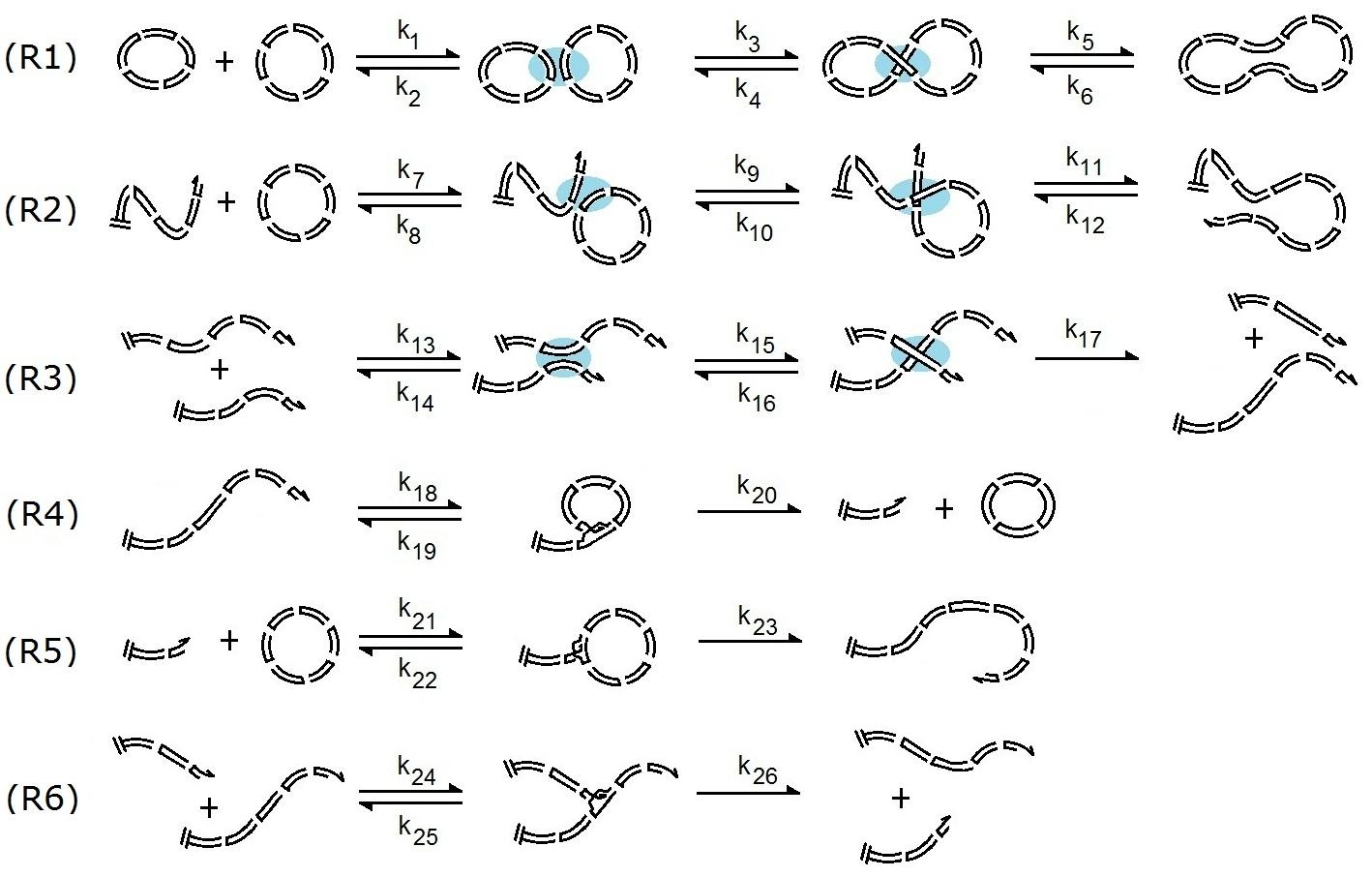
Figure 1: The full schematic list of reactions in the CTLY-model of ALT. The shadowed ovals represent transient recombination complexes. The reactions (R1)–(R3) represent recombination and dissociation while (R4)–(R6) represent end invasion and dissociation.

Based on the biophysical, biological, and mathematical assumptions described and justified in Section III.1 the full list of telomere interactions schematically displayed on Fig. 1 is constructed, see Section III.8 for more details about this so-called CTLY-model. Using the quasi-steady state approximation (see Section III.9) the system reduces to the CT-model described by Eqs. 1–2 where the kinetic rates are calculated from the biophysically derived rates for the CTLY-model (see Appendix B for details). Careful bookkeeping of the composition of the resulting rates in Eqs. 1–2 reveals that they satisfy detailed balance conditions and that the system equilibrium can be expressed by the explicit formulae

$$c_{n}=\frac{j(n)}{n}e^{-bn}\,,\ \ \ t_{n}=\frac{T}{V_{0}}(1-e^{-b})e^{-bn}\,,\ \ \ b>0,$$ (3)

where $T$ is the total number of t-arrays and $V_{0}$ is the volume of a sample (see Section IV.1).

The reduced C-model that only takes into account interactions of the t-circles (and neglects the interactions with t-arrays) has the form

$$\frac{dc_{n}}{d\tau} = \sum_{n>m>0}\left[k_{m,n-m}^{CC}c_{m}c_{n-m}-k_{m,n-m}^{C}c_{n}\right]$$ (4)

$$-\sum_{m>0}\left[k_{m,n}^{CC}c_{m}c_{n}-k_{m,n}^{C}c_{m+n}\right]\,.$$

It is introduced in Section III.10. Its equilibrium is given by

$$c_{n}=\frac{j(n)}{n}e^{-bn},\qquad b\geq 0\,.$$ (5)

Formulae in Eqs. 3 and 5 formally agree and show a good agreement with the experimental data (see Fig. 2). However, presence of population of t-arrays in Eq. 3 changes the value of the parameter $b$ that may dramatically change the system dynamics. This is due to the fact that for $b\geq 0$ the reduced t-circle model has an equilibrium of a maximal possible mass

$$M_{\text{max}}=V_{0}\sum_{n=1}^{\infty}nc_{n}=V_{0}\sum_{n=1}^{\infty}j(n),\qquad(b=0)\,,$$ (6)

while the equilibrium in Eq. 3 admits any finite mass for $b>0$. Furthermore, the reduced dynamics of t-circles in Eq. 4 allows gelation effect of non-zero mass in t-circles of infinite size, while such a phenomenon does not appear in Eqs. 1–2 (see Section IV.2 for more explanation).

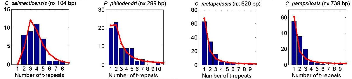
Figure 2: The comparison of the t-circle size distribution $\hat{c}_{n}$ predicted by the C-model and given by Eq. 5 with the experimental data (bar diagram). The total number of t-repeats and the total volume are $M=141$, $V_{0}=1.43\mu\text{m}^{3}$ (C. salmanticensis); $M=217$, $V_{0}=0.32\mu\text{m}^{3}$ (P. philodendri); $M=246$, $V_{0}=0.5\mu\text{m}^{3}$ (C. metapsilosis); and $M=228$, $V_{0}=0.5\mu\text{m}^{3}$ (C. parapsilosis).

Influence of species specific and experiment specific parameters on the telomere size distributions is studied in Sections IV.3 and IV.4. The concluding Section V discusses open questions and possible utilization of several different phenomena in applications and in further studies. Section III.11 contains an additional interesting problem related to experimental data. Finally, we point readers interested in analysis of the coagulation-fragmentation systems to Appendix C where they can find a review of the literature in the field. We note that the kinetic rates derived for interacting telomeres do not fit into any of the classes analyzed in the literature and thus the theoretical studies of the systems with these rates pose an interesting open problem (see Appendix C).

II Biological Background

II.1 Alternative Telomere Length Maintenance

The main mechanism that prevents shortening of chromosomal termini is based on the reverse transcriptase activity of the enzyme telomerase, the RNA-protein complex composed of the template RNA subunit and the protein catalytic subunit that extends the 3’ single-stranded telomeric overhang and thus prevents shortening of chromosomes Greider and Blackburn (1985, 1987). However, telomerase-mediated synthesis of chromosomal DNA is not the only mechanism of telomere maintenance Lundblad (2002). Examples of telomerase-independent pathways include (i) retrotransposition in Drosophila Pardue and DeBaryshe (2003), (ii) telomeric loops (t-loops) Griffith et al. (1999), (iii) chromosome circularization in mutant strains of both fission yeast Nakamura et al. (1998) and Streptomyces Qin and Cohen (2002), and in mitochondria of a number of yeast species Nosek et al. (1995); Rycovska et al. (2004), (iv) heterochromatin amplification-mediated telomere maintenance (HAATI) mechanism Jain et al. (2010), and (v) homologous recombination. The latter was elaborated mainly by studies on telomere maintenance in yeast McEachern and Blackburn (1996); Teng and Zakian (1999); Teng et al. (2000), but it was also found to operate in a wide variety of organisms including some insects, plants Biessmann and Mason (1997) and humans Dunham et al. (2000). Homologous recombination does not only help to maintain telomeres, but is also involved in generation of genomic plasticity and instability in the absence of telomerase, resulting in amplification or rapid deletion of telomeric DNA and in formation of extrachromosomal telomeric fragments Lundblad (2002); Niida et al. (2000). Homologous recombination in telomere dynamics is considered to be one of the hallmarks of telomerase-deficient cancer cell lines maintaining their telomeres via Alternative Lengthening of Telomeres mechanism (ALT) Cesare and Reddel (2010); Tomaska et al. (2009).

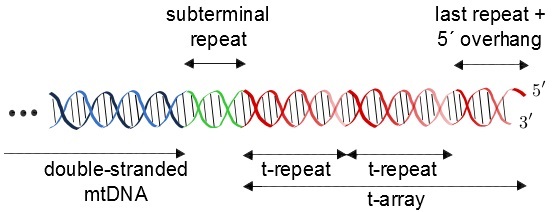
Figure 3: Telomere structure of the linear mtDNA in yeast C. parapsilosis.

II.2 Telomeric arrays and circles

Linear mitochondrial genome of the yeast C. parapsilosis carrying a standard set of mitochondrial genes is represented by population of double-stranded DNA molecules of the length 30,923 bp terminating on both sides by telomeres consisting of a subterminal repeat (554 bp) and a t-array of t-repeats ($n\times 738$ bp) (Fig. 3). Individual molecules in this population differ in size by the number of full-length t-repeats, ranging from 0 to at least 12. The shortest molecules (30,923 bp) terminate only with an incomplete tandem unit, while the termini of longer molecules are extended into t-arrays on both ends ($30,923+(n+m)\times 738$ bp, $m$ and $n$ are the numbers of full t-repeats in t-arrays of the left and right telomere, respectively). The very ends of the molecules have single-stranded 5’ overhangs of about 110 nucleotides (as opposed to 3’ overhangs that are typical for nuclear DNA), which in a fraction of molecules invade into the double-stranded region (end invasion) thus forming a duplex loop structure termed t-loop Tomaska et al. (2002). Single-stranded overhangs are believed to be associated with a recombination mode of replication of telomeres including nuclear telomeres Oganesian and Karlseder (2011).

Linear DNA molecules are accompanied by series of double-stranded circular molecules dubbed telomeric circles (t-circles). Their sizes correspond to integral multimers of the t-repeat with a length ($n\times 738$ bp). The circular molecules may originate from the t-loops and/or the t-arrays by recombination transactions followed by excision of a circle Tomaska et al. (2000). On the other hand, the t-circles were shown to replicate independently of the linear genomic molecules via rolling-circle mechanism leading to amplification of the linear arrays of t-repeats. Overall, they represent a substrate for recombinational mode of the mitochondrial telomere maintenance Nosek et al. (2005). Investigation of mutant cells lacking the t-circles revealed that they contain a circularized derivative of the genome. This supports the idea that the t-circles play a key role in the mechanism of telomere maintenance Tomaska et al. (2004); Kosa et al. (2006); Rycovska et al. (2004). This mechanism does not require telomerase activity; rather it relies on a relatively complex interplay among t-circles, lasso-shaped rolling-circle replication intermediates, t-loops and t-arrays.

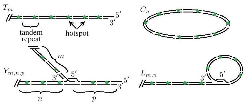
Figure 4: Telomeric structures participating in replication of linear mtDNA containing t-repeats: $T_{m}$ a t-array with $m$ t-repeats, and a 5’ single-stranded overhang, $C_{n}$ a t-circle with $n$ t-repeats. Also displayed are intermediate products $L_{m,n}$ a t-loop formed by an invasion of the 5’ overhang into the same telomeric strand of the total length $m+n$ t-repeats with the capping loop of the length $n$ t-repeats, and $Y_{m,n,p}$ a copy-choice structure (a triple junction) resembling a letter Y. Hotspots within each t-repeat are indicated by circles. The skew lines at the end of $T_{m}$, $Y_{m,n,p}$, and $L_{m,n}$ represent a chromosome not displayed on the figure.

Various simple types of telomeric structures are schematically illustrated on Fig. 4. Analogous telomeric structures (t-arrays, t-loops, t-circles) are associated with eukaryotic nuclear telomeres pointing to a general significance of the mitochondrial model Tomaska et al. (2009).

III Model and Data

III.1 Physical scales and assumptions

Biophysically and biologically feasible assumptions about the experimental environment and physical scales limit the types of structures and reactions involved in ALT and determine the constitution of the kinetic rates from biophysical components. The telomeric structures in the model are classified according to their length into classes of (see Fig. 4)

• t-arrays $T_{m}$, $m\geq 0$, with $m$ full t-repeats and a 5’ overhang,

• t-circles $C_{n}$, $n\geq 1$, with $n$ full t-repeats.

Two t-arrays located at different ends of a single chromosome are, for simplicity, considered to be two independent particles.

Physical scales. Detailed telomere and protein structure is necessary to unveil individual aspects of telomere length maintenance. However, to understand the size distributions of telomeres we focus on the coarse-grained spatial scale with a typical size of hundreds of nanometers on which we distinguish size, type, and shape of individual telomeres but ignore their nucleotide sequence. The typical time scale is set to one second, the time scale short for DNA degradation, cell division, and for a significant contribution of synthesis of new t-repeats via the rolling-circle mechanism. Despite the fact that conservation of the total number of t-repeats valid on the fast time scale breaks down on a longer time scale commensurate with laboratory experiments, we argue that the measurements at each instance display “an equilibrium distribution” for the actual number of t-repeats, i.e., a quasi-steady state.

Assumptions. The assumptions underlying the model can be divided into three classes: assumptions on biology and biophysics of the system, and mathematical assumptions.

The assumptions on the biology are (i) all telomeres are double-stranded with the exception of a single-stranded overhang; (ii) more complex telomeric structures than those considered are dynamically unstable; (iii) there is only one specific reactive group, hotspot, per t-repeat that is susceptible to homologous recombination; (iv) there is an abundance of binding proteins in the environment, i.e., availability of proteins does not limit local reaction rates that can be then viewed as crossings of energy barriers.

The assumptions (i) and (ii) were validated by the study Tomaska et al. (2009) where no other telomeric structures were observed. That can be interpreted either as a lack of other types of structures or a sign of their dynamical instability. The assumption (iii) is not essential for our work, and in general, more hotspots of different structure may be active within one t-repeat. The structure of hotspots within one t-repeat only affects a single parameter of our problem ($g_{1}$) that may be species dependent; it only influences the time scale of convergence to equilibrium telomere size distributions and does not alter their shape.

The assumption (iv) is typical in the Kramer’s theory; a widely accepted theory of local chemical interactions. In the particular laboratory experiments that correspond to the biological system we study the yeast cells were held under normal physiological conditions and thus binding proteins are expected to be available in equilibrium concentrations. Also, any variation of their concentration would only change the values of the correction factors $g_{1},g_{0}$ and $g_{-1}$, i.e., our results once again show that it has no influence on the shape of the resulting telomere size distributions.

The assumptions on the system biophysics are (v) telomeres are well-mixed and are freely diffusing in a homogeneous three-dimensional confinement at a constant temperature; and (vi) telomeres do not have super-helical structure and do not interact with such super-coiled structures.

The assumption (v) is an assumption commonly used in chemical kinetics; it allows to describe the dynamics in a form of a system of ordinary differential equations rather than physically more realistic partial differential equations. In the absence of a fluid flow motion of telomeres in an aquatic solution is governed by diffusion and elastic forces within the DNA. Despite the possibility that a tangled geometry of mitochondria may strongly influence diffusivity and bending of telomeres, small dimensions of telomeres (particularly of hotspots) motivate us to neglect such a spatial inhomogeneity. The issue of possible differences in a behavior of a single cell vs. cell population is addressed in Section V.

The assumption (vi) is certainly violated in the biological systems as various experimental studies show presence of telomeres of both relaxed and super-coiled geometries. Although the super-coiled molecules have different diffusive and reactive properties from the relaxed geometry telomeres considered here, they, according to the experiments, only account for a small fraction of telomeric structures. Here, for simplicity we neglect their presence and their effect on the telomere size distributions will be a subject of our further research.

Obviously, in a real environment none of these biological and biophysical assumptions is exactly satisfied, nevertheless, we assume that their failure does not significantly change the qualitative behavior of the system.

We put forward also one mathematical assumption. We describe population dynamics of telomeres by a system of ordinary differential equations that, in general, requires large enough populations. However, in our application population levels of telomeres with a large number of t-repeats are typically small. We believe that the good agreement of predictions of our model with experimental data provides its justification, although an extreme caution is necessary in interpretation of the results for populations of long telomeres.

III.2 Reaction rates

The repetitive structure of telomeres restricts their interactions to three types: homologous recombination, end invasion, and dissociation (Fig. 1). Homologous recombination in reactions (R1)–(R3) requires proximity of two identical spatially aligned hotspots on the same strand or on two different strands. Under favorable conditions (availability of recombination proteins, etc.) a transient complex is formed resulting either in an original configuration of strands or in an exchange of nucleotide sequences between the strands.

While homologous recombination is a reaction of two identical reacting groups (hotspots), end invasion in reactions (R4)–(R6) is an insertion of the single-stranded overhang located at the terminus of a DNA strand into the same or another strand. Invasion into the same t-array produces a capped form of a telomere (t-loop) while invasion into a different t-array yields a copy-choice structure (triple junction) (Fig. 4). Again, the repetitive structure of the telomeres implies that each single-stranded overhang is only able to invade a specific location within a t-repeat that contains a region with identical sequence as the overhang.

According to the Kramer’s theory Jackson (2006) even under favorable conditions each local interaction of telomeres requires crossing of an energy barrier that effectively reduces the overall rate by a reaction-rate limited factor. The overall kinetic rates of individual reaction types of telomere interactions have the following structural decomposition:

• bimolecular association of free particles

  $$r=\begin{pmatrix}\text{diffusion}\\ \text{lim.~{}rate}\end{pmatrix}\times\begin{pmatrix}\text{comb.}\\ \text{factor}\end{pmatrix}\times\begin{pmatrix}\text{reaction--rate}\\ \text{lim.~{}factor}\end{pmatrix}\,,$$

• unimolecular self interaction (association of two groups of the same reactant)

  $$r=\begin{pmatrix}\text{diffusion}\\ \text{lim.~{}rate}\end{pmatrix}\times\begin{pmatrix}\text{comb.}\\ \text{factor}\end{pmatrix}\times\begin{pmatrix}\text{reaction--rate}\\ \text{lim.~{}factor}\end{pmatrix}\times\begin{pmatrix}\text{J-factor}\end{pmatrix},$$

• dissociation

  $$r=\begin{pmatrix}\text{diffusion}\\ \text{lim.~{}rate}\end{pmatrix}\times\begin{pmatrix}\text{reaction--rate}\\ \text{lim.~{}factor}\end{pmatrix}/{\begin{pmatrix}\text{reaction}\\ \text{volume}\end{pmatrix}}\,.$$

The individual constituents are: (a) the diffusion limited rate that measures the rate at which two molecules encounter each other if driven only by a molecular diffusion; (b) the combinatorial factor that accounts for the number of different configurations of reactants in a reaction yielding the same product; (c) the reaction-rate limited factor that accommodates reaction-limited interactions for homologous recombination and end invasion; (d) the J-factor that accounts for bending of a polymer in terms of a local molar concentration of a reactive group at a given site; and (e) the reaction volume.

III.3 Diffusion limited rate

Diffusion limited kinetic rates Robertson et al. (2006); Jackson (2006) are determined by the size and the shape of reacting molecules. Dependence of the rate on the polymer size is often suppressed in modeling of telomere interactions Olofsson and Bertuch (2010); Rodriguez-Brenes and Peskin (2010) in agreement with the classical theory of Flory (1953) that suggests to neglect such an effect. Hence we visualize every telomeric structure with $n$ full t-repeats as $n$ independent recombination hotspots each with the same diffusive properties of a single hotspot. Analogous view is used for the single-stranded overhang and corresponding matching sequences within each t-repeat. For simplicity, we do not distinguish between these two cases as we expect the length of the reactive group to be approximately the same (about 10 bp) for both recombination and end invasion. However, note that the single-stranded overhang is expected to have higher mobility (and thus different diffusive properties) than the double-stranded hotspot. To simplify the presentation and to streamline the parameter dependencies we include such an effect into the reaction-rate limited factor that condenses the various differences between recombination and end invasion (see Section III.5).

The Smoluchowski theory Robertson et al. (2006) predicts the kinetic rate of a bimolecular reaction of two freely diffusing spherical molecules $A$ and $B$ to be

$$k_{D}(A,B)=4\pi D(A,B)r(A,B)$$ (7)

with the joint diffusion coefficient $D(A,B)=D(A)+D(B)$ and the joint molecular radius $r(A,B)=r(A)+r(B)$. The diffusion coefficient $D(A)$ of a spherical molecule $A$ depends on its physical parameters and on the environment via the Stokes-Einstein formula

$$D(A)=\frac{k_{B}T_{\text{a}}}{6\pi\hat{\nu}r(A)}\,,$$ (8)

where $k_{B}$, $T_{\text{a}}$, $\hat{\nu}$ and $r(A)$ are the Boltzmann constant, the absolute temperature, solvent viscosity, and the radius of the molecule $A$, respectively. Equations 7 and 8 yield the bimolecular diffusion limited reaction rate of two hotspots

$$k:=k_{D}(H,H)=\frac{8k_{B}T_{\text{a}}}{3\,\hat{\nu}}\,.$$

Note that the rate is independent of the dimensions of the hotspot indicating a universal rate for two identical molecules in agreement with the well-known observation of Jacobson and Stockmayer (1950). The effective reaction volume of two interacting hotspots is given by

$$V:=V(H,H)=\frac{4}{3}\pi r(H)^{3}\,,$$

where $r(H)$ is the effective radius of a hotspot $H$. However, in our model none of the parameters $k$, $V$, and $r(H)$ has an impact on the telomere equilibrium size distribution as they only influence the overall time scale of convergence of the distribution to the equilibrium, see Section III.9.

III.4 Combinatorial Factor

Since recombination of any two hotspots on two different t-circles of the classes $C_{m}$ and $C_{n}$ (or alternatively on a t-circle $C_{n}$ and a t-array $T_{m}$) yields the same complex (reactions (R1) and (R2) in Fig. 1), the combinatorial factor accounting for the number of possible pairs of reacting hotspots is a product $mn$ (Fig. 5A). The combinatorial factor for an interaction of two recombination hotspots on a single t-circle $C_{m+n}$ is equal to the total number $m+n$ of hotspots on the t-circle for all possible recombination complexes (Fig. 5B).

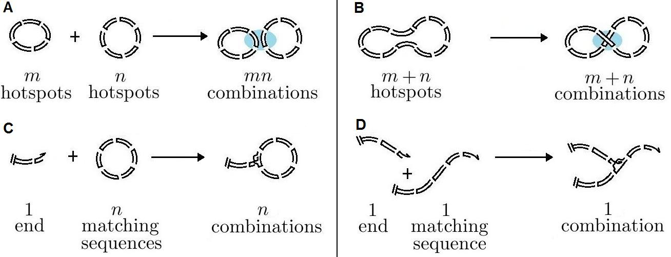
Figure 5: (A) Recombination of $C_{m}$ and $C_{n}$ yields the identical recombination complex for all $mn$ choices of pairs of interacting hotspots. (B) Self recombination of two hotspots on $C_{m+n}$ yields the identical recombination complex for $m+n$ choices of pairs of interacting hotspots at the distance $m$ (or $n$) t-repeats along the t-circle. (C) End invasion of $T_{m}$ into $C_{n}$ with $n$ choices. (D) End invasion of $T_{m}$ into $T_{n}$ with only one choice of the interacting site for each type of the complex.

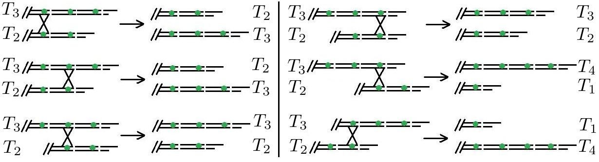
Figure 6: Recombination of t-arrays. Different outcomes of recombination of t-arrays $T_{3}$ and $T_{2}$ are schematically displayed. Two combinations lead to $T_{2}$ and $T_{3}$ and one combination leads to $T_{1}$ and $T_{4}$. Similarly, two combinations produce $T_{3}$ and $T_{2}$ and one produces $T_{4}$ and $T_{1}$. In general, $\min(m,n,p,m+n-p)$ combinations of recombination hotspots of $T_{m}$ and $T_{n}$ result in $T_{p}$ and $T_{m+n-p}$.

Recombination of two hotspots on two distinct t-arrays yields different types of recombination complexes (Fig. 6). A simple calculation reveals that there are $\min(m,n,p,m+n-p)$ different pairs of hotspots on $T_{m}$ and $T_{n}$ that yield a recombination complex which after an exchange of ends decomposes into $T_{p}$ and $T_{m+n-p}$.

On the other hand, end invasion requires participation of the single-stranded overhang in the interaction eliminating a part of the combinatorial factor. Each t-repeat on the invaded telomeric strand has one specific matching sequence. The overall combinatorial factor of end invasion of a t-array into $C_{n}$ and $T_{n}$ is thus $n$ and 1, respectively (see Figs. 5C and 5D).

III.5 Reaction-Rate Limited Factor

A reaction-rate limited factor accounts for the fact that two molecules within the reactive distance have to overcome an additional potential barrier to react Jackson (2006); Phillips et al. (2009). Note that this factor may also include a cumulative effect of an availability of connecting proteins facilitating interactions, a presence of a capping protein attached to the single-stranded overhang Rodriguez-Brenes and Peskin (2010), and enhanced diffusion of single-stranded DNA.

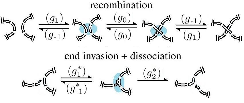
Figure 7: Schematic diagrams of local interactions: recombination, end invasion and dissociation of telomeric structures. The reaction-rate limited correction factors are indicated.

The Noyes theory Noyes (1961) identifies the second order correction $\kappa$ that affects the diffusion-limited reaction rate and can be interpreted as a barrier crossing:

$$k_{N}(A,B) = k_{D}(A,B)\frac{\kappa}{k_{D}(A,B)+\kappa}=k_{D}\left(1+\frac{k_{D}}{\kappa}\right)^{-1}$$ (9)

$$\approx k_{D}\exp(-\triangle G/k_{B}T_{\text{a}})=k_{D}g\,,$$

where $g:=\exp(-\triangle G/k_{B}T_{\text{a}})$. Equation 9 defines the energy barrier $\triangle G$ and the correction factor $g$ of a particular reaction. The correction factors $g_{1},g_{0},g_{-1}$ are associated with recombination, and $g^{\ast}_{1},g^{\ast}_{2},g^{\ast}_{-1}$ are associated with end invasion (see Fig. 7 for a schematic display).

III.6 J-factor – the measure of DNA looping

Looping of DNA strands plays an important role in internal cell regulation and particularly in gene regulation. Passive diffusive motion leads to a DNA strand configuration that is favorable for creation of a link between its two sections (often in presence of a binding protein). The well studied examples are regulation of Lac repressor Towles et al. (2009) and gal operon Allemand et al. (2006) that block DNA transcription. In both cases, the DNA loop is site-specific and it does not detach from the strand. Another example of site-specific looping is recombination Allemand et al. (2006) involving Cre protein connecting two loxP sites that leads to an excision of a circular DNA fragment that regulates gene switching.

The problem of DNA looping has attracted a lot of attention in scientific community since the publication of the seminal paper of Jacobson and Stockmayer (1950) that introduced the so-called J-factor. The traditional approach is based on the worm-like chain (WLC) polymer model of Kratky and Porod (1949), although alternative biophysical and computational methods are used as well. In 1980s a series of biological experiments conducted by Shore et al. (1981) and a theoretical essay by Shimada and Yamakawa (1984) lied down a theoretical framework for the subject that was further tested in numerical simulations. A qualitative difference between DNA looping in vivo and in vitro for short strands was pointed out by Ringrose et al. (1999) who proposed an introduction of apparent persistence length for DNA polymers in vivo as a consequence of a presence of chromatin. Review papers Rippe et al. (1995); Allemand et al. (2006); Vologodskii (2009) provide a long list of literature on looping of linear DNA. The theory of circular (double) constrained looping is developed in Bloomfield (1974); Rippe (2001); Podtelezhnikov et al. (2000); Hanke and Metzler (2003).

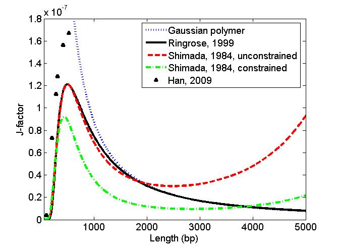
Figure 8: The values of J-factor measured in units of $\text{M}=1\,\text{mol}\cdot\text{dm}^{-3}$ in various models.

A disagreement in the extent of a couple of orders of magnitude was observed between values of $J$-factor in vivo and in vitro Han et al. (2009); Ringrose et al. (1999) (Fig. 8) and between in vivo values and theoretically computed values, particularly for lengths shorter than 100 bp (see the diagram (Towles et al., 2009, Fig. 10)). These differences were explained in Saiz and Vilar (2006) and studied analytically and numerically in a particular case of LacI repressing in Towles et al. (2009). The same group conducted further experiments and compared their calculations with theoretical predictions Han et al. (2009). Their results were recently supported by experimental study of Vafabakhsh and Ha (2012), see also Nelson (2012), pointing out the failure of the WLC model for looping of short DNA fragments.

The linear J-factor expresses availability of a given site in a neighborhood of another site in terms of a local molar concentration ($\text{M}=1\text{mol}\cdot\text{dm}^{-3}$)

$$k_{J}=j(L)k_{D}\,,$$ (10)

where $k_{D}$ is the kinetic rate of the appropriate bimolecular reaction Shore et al. (1981); Sanchez et al. (2011) and $L$ is the distance of the reacting hotspots along the DNA strand measured in bp .

Three types of DNA looping that may lead to an excision of a t-circle appear in ALT with their corresponding J-factors: (i) $j(L)$, linear constrained looping—recombination of two hotspots of a single t-array; (ii) $j^{\ast}(L)$, linear unconstrained looping—end invasion into the same t-array; (iii) $j(L_{1},L_{2})$, circular constrained looping—recombination of two hotspots of a single t-circle. Due to the disagreement in the literature it is not completely clear which values of J-factor apply in the setting of telomeres in yeast mtDNA. The t-repeats of mtDNA of the studied species of yeast (with the exception of C. salmanticensis) have lengths much longer than the persistence length of double-stranded DNA ($\ell_{p}=50$ nm) and the lengths of t-arrays cover a wide range ($0.1$–$10$ kbp). Thus, for simplicity, we use the linear J-factor values of Ringrose et al. (1999) (Fig. 8)

$$j(L)=\frac{1.25\times 10^{5}}{\ell_{p}^{3}}\,\left(\frac{4\ell_{p}}{10^{4}L}\right)^{1.5}\exp\left(\frac{-460\,\ell_{p}^{2}}{6.25L^{2}}\right)\,,$$ (11)

for both constrained and unconstrained linear looping ($j(L)=j^{\ast}(L)$). The model in Eq. 11 agrees for lengths over 2 kbp with the Gaussian polymer model

$$j_{G}(L)=1.66\,\left(\frac{3}{4\pi L\ell_{p}}\right)^{1.5}\,.$$ (12)

The rate of circular looping (circular J-factor) appears in the backward reaction (R1) (Fig. 1). The circular J-factor $j(m,n)$ measures the likelihood of looping of a DNA strand in situations when two particular hotspots on the same t-circle of a length $m+n$ t-repeats at a distance $m$ (or $n$) t-repeats along the t-circle form a recombination complex that can be upon successful recombination resolved into t-circles $C_{m}$ and $C_{n}$. Both lengths $m$ and $n$ contribute to the J-factor through the total entropy and elastic energetic loss. Under assumption of relaxed t-circle geometry, we use the detail balance condition Rippe (2001); Hanke and Metzler (2003)

$$j(L_{1},L_{2})=\frac{j(L_{1})j(L_{2})}{j(L_{1}+L_{2})}\,.$$ (13)

We have considered various other alternatives for both linear and circular J-factor (see Section V for more details) but the variation either did not significantly alter the results or it led to a disagreement with the experimental data.

III.7 Dissociation

In the case of diffusion limited dissociation kinetic rates are determined by diffusive properties of the molecules Jackson (2006). The rate of dissociation $k_{d}$ of spherical molecules $A$ and $B$ with effective radii $r(A)$ and $r(B)$ in the case of very weak attractive forces is given by

$$k_{d}(A,B)=\frac{3D(A,B)}{r(A,B)^{2}}=\frac{k_{D}(A,B)}{V(A,B)}\,.$$

If the interaction potential between the molecules is $U(r)$ (the related attractive force is $dU(r)/dr$) then the dissociation rate is given by

$$k_{dU}=\frac{3De^{U(r)/k_{B}T_{\text{a}}}}{r^{3}\int_{r}^{\infty}\exp(U(\rho)/k_{B}T_{\text{a}})/\rho^{2}\,d\rho}=\frac{k_{D}}{V}g\,,$$ (14)

where arguments $(A,B)$ are suppressed. The correction factor $g$ can be interpreted in terms of the Kramer’s theory as an energy barrier of height $\Delta G_{d}$ (see also Eq. 9):

$$k_{d}(A,B)=\frac{k_{D}(A,B)}{V(A,B)}\exp\left(\frac{-\Delta G_{d}}{k_{B}T_{\text{a}}}\right)\,.$$

Strongly diffusion limited dissociation corresponds to $U(r)\equiv 0$ in Eq. 14 and $\Delta G_{d}=0$, analogously to strongly diffusion limited association by recombination ($\kappa=\infty$, Eq. 9) where $\Delta G=0$.

III.8 CTLY-model

Figure 1 schematically displays interactions (R1)–(R6) of telomere structures: t-arrays, t-circles, t-loops, triple junctions, and recombination complexes, in our most complex model of ALT, dubbed the CTLY-model. Although telomere structures of arbitrary length make the size of the system virtually infinite, the conservation of the total number of t-repeats in the system effectively bounds the maximal telomere size.

Telomere interactions in the CTLY-model are homologous recombination of t-arrays and t-circles in reactions (R1)–(R3), and end invasion of a t-array into the same or another t-array or t-circle in (R4)–(R6) (see Fig. 1). Intermediate complexes are subsequently formed in (R1)–(R3) reflecting the three-stage process: approach of the two reactive parts, local protein mediated recombination, and dissociation. Due to the assumption of limited reactivity of the intermediate complexes we assume that they do not self-interact or recombine, neither they are invaded by telomeric overhangs to form more complex structures (double circles, quadruple junctions, etc.).

The rates in the CTLY-model can be directly deduced from the above discussion. Let $n$ and $m$ be the numbers of t-repeats in particular t-circles and t-arrays involved in the reactions in the CTLY-model displayed on Fig. 1. The association kinetic rates are given by

$$k_{1} = k_{1}(C_{n},C_{m})=k_{7}=k_{7}(T_{m},C_{n})=mnkg_{1}\,,$$

$$k_{6} = k_{6}(C_{m},C_{n})=(m+n)j(n,m)kg_{1}\,,$$

$$k_{12} = k_{12}(T_{m},C_{n})=mj(n)kg_{1}\,,$$

$$k_{13} = k_{13}(T_{m},T_{n},T_{p})=\min(m,n,p,m+n-p)kg_{1}\,,$$

$$k_{18} = k_{18}(T_{m},C_{n})=j^{\ast}(n)kg^{\ast}_{1}\,,$$

$$k_{21} = k_{21}(T_{m},C_{n})=nkg^{\ast}_{1}\,,$$

$$k_{24} = k_{24}(T_{m},T_{n})=kg^{\ast}_{1}\,.$$

The arguments $C_{n}$ and $T_{m}$ are specified in such a way that the reaction is uniquely identified although the particular molecules do not need to participate in it (as in $k_{6}$, the indexes $m$ and $n$ identify the lengths of the looped arcs created in the recombination complex). The rate $k_{13}$ requires the information on the product of the recombination complex $T_{p}$ (and complementary $T_{m+n-p}$). The dissociation rates are

$$k_{2}=k_{5}=k_{8}=k_{11}=k_{14}=k_{17}=kg_{-1}/V,$$

$$k_{3}=k_{4}=k_{9}=k_{10}=k_{15}=k_{16}=kg_{0}/V\,,$$

$$k_{19}=k_{22}=k_{25}=kg^{\ast}_{-1}/V\,,\quad k_{20}=k_{23}=k_{26}=kg^{\ast}_{2}/V.$$

III.9 Reduction to CT-model

The quasi-steady state approximation (QSSA) Atkins (1994); Eigen (1974) provides a reduction of reaction kinetics when a replacement of some of differential equations in the system by their equilibria does not significantly alter the dynamics of the whole system on a specifically considered time scale. The selected components in “equilibrium” are often called slaved variables as their approximated dynamics is slaved to the rest of the system by an algebraic law expressing the equilibrium. Validity of such an approximation can be justified using the mathematical technique of singular perturbation Segel and Slemrod (1989); Schnell and Maini (2003); Tzafriri and Edelman (2005) under an assumption of a separation of time scales, specifically under overall imbalance of association and dissociation. While the use of the QSSA can be more-or-less justified for every individual reaction displayed schematically on Fig. 1, the validity needs to be justified for the full system of reactions simultaneously. Unfortunately, the existing theory does not cover such a case and thus it poses an interesting and difficult open mathematical problem. Nevertheless, here we apply the QSSA in the CTLY-model as our numerical simulations suggest its validity.

The QSSA reduces the CTLY-model to the CT-model:

$$C_{m}+C_{n} \autorightleftharpoons{\small$k^{CC}$}{\small$k^{C}$} C_{m+n}\,,$$ (15)

$$T_{m}+C_{n} \autorightleftharpoons{\small$k^{TC}$}{\small$k^{T}$} T_{m+n}\,,$$ (16)

$$T_{m}+T_{n} \autorightarrow{\small$k^{TT}$}{} T_{p}+T_{m+n-p}\,,$$ (17)

where reaction (R1) (see Fig. 1) was reduced to Eq. 15, reactions (R2), (R4) and (R5) were reduced and added up to Eq. 16, and similarly reactions (R3) and (R6) were reduced and added up to Eq. 17. More details on the QSSA and on the explicit reduction to Eqs. 15–17 can be found in Appendix B.

After rescaling of the time variable $\tau=\hat{k}tg_{1}$ the kinetic rates in Eqs. 15–17 are

$$k^{CC}_{m,n} = k^{CC}(C_{m},C_{n})=mn,$$

$$k^{C}_{m,n} = k^{C}(C_{m},C_{n})=(m+n)j(m,n)\,,$$

$$k^{TC}_{m,n} = k^{TC}(T_{m},C_{n})=n(m+\alpha),$$ (18)

$$k^{T}_{m,n} = k^{T}(T_{m},C_{n})=j(n)(m+\alpha)\,,$$

$$k^{TT}_{m,n,p} = k^{TT}(T_{m},T_{n},T_{p})=\min(m,n,p,m+n-p)+\alpha\,.$$

The non-dimensional parameters characterizing the relative strength of the energy barriers of the local interactions, and the rescaled diffusion coefficient $k$ are given by

$$\beta=\frac{g_{-1}}{g_{0}},\ \ \gamma=\frac{g_{-1}^{\ast}}{g_{2}^{\ast}}\,,\ \ \alpha=\frac{(1+\gamma)g_{1}^{\ast}}{(2+\beta)g_{1}},\ \ \hat{k}=\frac{k}{2+\beta}.$$ (19)

The resulting (infinite) system of differential equations in Eqs. 1–2 describes time evolution of the concentrations $c_{m}$ and $t_{n}$ of the populations of $C_{m}$ and $T_{n}$, $m>0,n\geq 0$, in the sample solvent.

The continuous quantities $c_{m}$ and $t_{n}$ can be interpreted as statistical measures (number densities) of populations of telomeres of type $C_{m}$ and $T_{n}$ in the sample, or (particularly in the case of their value smaller than one) as probabilities of an occurrence of an element of the given type in the sample. The actual number of particles of a given class is given by $\hat{t}_{m}=V_{0}t_{m}$ and $\hat{c}_{n}=V_{0}c_{n}$, where $V_{0}$ is the sample volume. Important conserved quantities of the CT-model are the total number of t-repeats (total mass) $M$ and the total number of t-arrays $T$ in the system. Also, $M=M_{C}+M_{T}$, where $M_{C}$ and $M_{T}$ are the total numbers of t-repeats in t-circles and t-arrays in the sample, respectively:

$$M_{C}=\sum_{n=1}^{\infty}n\hat{c}_{n}\,,\ \ M_{T}=\sum_{n=1}^{\infty}n\hat{t}_{n}\,,\ \ T=\sum_{n=0}^{\infty}\hat{t}_{n}\,.$$ (20)

III.10 Reduction to C-model

Equations 18 reveal that there is no time scale separation between interactions of t-circles with themselves and mutual interactions of t-circles and t-arrays. Nevertheless, due to the particular structure of Eqs 1–2 it is possible to study a reduction of Eqs. 1–2 to account only for interactions of t-circles. Absence of linear telomeres ($t_{n}=0$ for $n\geq 0$) reduces the dynamics of the CT-model to the C-model described by Eq. 4. The kinetic rates $k^{CC}$ and $k^{C}$ remain unchanged and they are given by Eqs. 18. The main advantage of this reduced C-model is that it fits to an existing mathematical framework of coagulation-fragmentation Aizenman and Bak (1979); Bak and Bak (1959); Ball and Carr (1990); Da Costa (1995), although the reaction rates do not fall directly into classes studied theoretically up to this date.

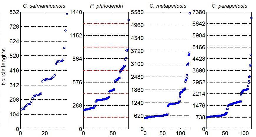
Figure 9: Apparent experimentally measured lengths of t-circles ordered by size (in bp). Multiples of sizes of t-repeats of individual yeast species are indicated by horizontal lines. Additional lines at half of the t-repeat length are shown for P. philodendri. Clustering of t-circles may be observed for all species, however, the gap between clusters in case of P. philodendri is approximately half of the length of the t-repeat (288 bp).

III.11 Data binning

In reported experimental data Tomaska et al. (2000) obtained by electron microscopy (see Appendix A for details) length of multiple t-circles was located far from its expected value (an integer multiple of the length of the corresponding t-repeat). One can attempt to categorize the t-circles according to their nearest multiple of the t-repeat length but due to the high length variability it is difficult to assign them into a proper size distribution bin. However, the actual t-circle size distributions display an emerging feature illustrated on Fig. 9. They are naturally clustered to groups with well separated lengths corresponding to classes of t-circles with different integer numbers of t-repeats. Based on this natural clustering we have rejected the original binning method of Tomaska et al. (2000) and classified the t-circles according to the clusters recounted directly from the experimental electron microscopy data. The clusters of C. metapsilosis and C. parapsilosis are relatively easy to classify with measurement precision decreasing as the t-circle size grows. Unfortunately, it is unclear how should be some of the clusters associated to the number of t-repeats, particularly in the case of C. salmanticensis. Also, P. philodendri with t-repeat size 288 bp has the gap between clusters approximately halved in contrast with other yeast species where the cluster gaps match the t-repeat size.

Based on the observation of clusters of the other yeast species we have categorized the first cluster of the t-circles of C. salmanticensis with apparent t-circle sizes between 104 bp and 208 bp as t-circles with two full t-repeats, i.e., we conjecture that there is no t-circle with one t-repeat. The main argument is that we expect that the apparent length of a planar microscopic image of a t-circle underestimates the actual t-circle length due to the two-dimensional projection and it cannot by any means significantly extend the expected t-repeat size. Further clusters of t-circles of C. salmanticensis are categorized accordingly. The clusters of P. philodendri were categorized as $C_{1}$, $C_{2}$, etc., despite the smaller cluster gap.

IV Results

Three models with a decreasing level of complexity were constructed using the approach described in Section III: the CTLY-model, the CT-model, and the C-model. The most complex CTLY-model was studied only through numerical simulations that confirmed the validity of the QSSA. The experimental data were matched with the explicit equilibria of the CT-model and the C-model. Furthermore, we performed parametric studies of the CT-model to detect the system response to parameters and analyzed the C-model rigorously using the mathematical theory of coagulation-fragmentation equations.

IV.1 Distribution of t-circles

C-model. The expected size distribution of the t-circles $\hat{c}_{n}$ with $n$ full t-repeats in the C-model is an equilibrium of the system of Eqs. 4, $n\geq 1$ . Due to the structure of the kinetic rates and the fact that the circular J-factor satisfies the detailed balance condition in Eq. 13 the equilibrium can be explicitly calculated as

$$\hat{c}_{n}=V_{0}\frac{j(n)}{n}e^{-bn}\,,$$ (21)

where $b\geq 0$ is a parameter that is uniquely determined by $M=M_{C}$. The quantity $M_{C}$ is experiment specific but it was not measured in experiments as the protocol does not guarantee detection of all telomeres in a sample. As expected the equilibrium distribution of t-circles in this simple approximation strongly depends on the individual species t-repeat length (through the J-factor) with shorter telomeres more difficult to bend and longer (pliable) telomeres with smaller tendency for circularization because of a small probability of a proper alignment of the specific reactive sites (entropy effects). Thus, according to Eq. 21 the J-factor appears to be the main source of the difference between the character of the data for different yeast species. A comparison of the data with the C-model predictions of t-circle size distributions for four distinct yeast species is displayed on Fig. 2. The same parameters were used for matching except the individual length of telomeric repeat and the experiment specific total number of t-repeats $M$ and the sample volume $V_{0}$ that were determined by minimization of the sum of squared error (SSE). All optimal values of $M$ and $V_{0}$ lie within an expected range.

CT-model. Similarly, the equilibrium of the CT-model in Eqs. 1–2 can be explicitly calculated as:

$$\hat{c}_{n}=V_{0}\frac{j(n)}{n}e^{-bn}\,,\ \ \ \hat{t}_{m}=T(1-e^{-b})e^{-bm}\,,\ \ \ b>0.$$ (22)

Therefore, the expected distribution of t-arrays is exponentially decaying with the same rate of exponential decay as the rate of decay of the distribution of t-circles (Fig. 10). On the other hand, the J-factor does not directly influence the size distribution of t-arrays, except through the value of parameter $b$. A quick comparison of Eqs. 21 and 22 reveals that the size distributions of t-circles in the C-model and the CT-model agree although the parameter $b$ may be different. Also, both $\hat{c}_{n}$ and $\hat{t}_{m}$ are independent of $\alpha$, i.e., telomere interactions via end invasion do not alter the telomere size distributions. The parameter $b$ is uniquely determined by the total number of t-repeats (in t-arrays and t-circles) in the system (Eq. 20)

$$V_{0}\sum_{n=1}^{\infty}j(n)e^{-bn}+T(1-e^{-b})\sum_{n=0}^{\infty}ne^{-bn}=M.$$ (23)

The second sum can be simplified and Eq. 23 reduces to

$$V_{0}\sum_{n=1}^{\infty}j(n)e^{-bn}+\frac{T}{1-e^{-b}}=M.$$ (24)

Two parameters (e.g. $V_{0}/M$ and $T/M$) are needed to determine the value of $b$ but the value of all three experiment specific parameters $V_{0},T$ and $M$, is needed for the distribution of $\hat{c}_{n}$ and $\hat{t}_{m}$ given by Eq. 22. We refer the reader to Appendix C for additional information on mathematical analysis of coagulation-fragmentation system in Eqs. 1–2 that extends existing results in the literature.

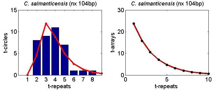
Figure 10: The distribution of t-circles and t-arrays of C. salmanticensis in the CT-model given by Eq. 22. While the distribution of t-circles is not monotone (the model prediction is compared with the bar diagram of experimental data), the size distribution of t-arrays is exponentially decaying. The parameters used are $T=50$, $V_{0}=1\mu\text{m}^{3}$, and $M=292$ that reduces to $M_{C}=92$.

IV.2 Excess mass

If the total number of t-repeats $M$ in the C-model is too large, the equilibrium distribution in Eq. 21 displays an interesting feature—excess mass. The key observation is that among all equilibria given by Eq. 21 there is one of the maximal finite mass $M_{\text{max}}$ (see Eq. 6). If the initial condition prescribes $M$ too large, $M>M_{\text{max}}$, to be accommodated by any finite mass equilibrium ($b\geq 0$) the extra (excess) mass is gradually transfered to higher and higher modes. Thus, the probability of a presence of larger and larger t-circles in the sample is increasing, while the distribution of telomeres of all sizes converges pointwise to the equilibrium of the largest possible mass $M_{\text{max}}$. Such a case happens generically any time the total count of t-repeats exceeds a critical value $M_{\text{max}}$, and in mathematical analysis it is connected with weak convergence. For the J-factor given by Eq. 11 that means an algebraic decay of the size distribution in Eq. 21 instead of an exponential decay. Presence of the numerically observed excess mass in the C-model was also confirmed for the kinetic rates that lie out of the range studied so far by rigorous mathematical analysis of Carr (2012).

IV.3 Species–specific parameters

T-repeat length is a species-specific parameter that influences telomere looping frequency and thus appears to be central for the distribution of the t-circles through the J-factor values (see Eq. 21). On the other hand, the diffusive properties of telomeres influence only the overall time scale of the size distribution dynamics with no further effect on the equilibrium.

In addition to these well identified dimensional parameters with known values the kinetic rates in the C-model and CT-model depend also on three non-dimensional local molecular parameters $\alpha$, $\beta$, and $\gamma$ defined by Eq. 19. They characterize relative sizes of the correction factors to the diffusion-limited kinetic rates in the individual reactions depicted on Fig. 7 that may be species dependent. The ratio of correction factors to diffusion-limited kinetic rates in recombination/end invasion and dissociation of a recombination/invasion complex is denoted $\beta$ and $\gamma$, respectively. The parameter $\alpha$ depends on the ratio of correction terms to diffusion-limited kinetic rates of end invasion and homologous recombination. The overall time scale of dynamics of the system is determined by $g_{1}\hat{k}=g_{1}k/(2+\beta)$.

IV.4 Experiment–specific parameters

There are three experiment specific parameters that enter into the model: $V_{0}$, $M$, and $T$. These parameters influence the equilibrium distributions $\hat{c}_{n}$ of t-circles (C-model) and of t-circles $\hat{c}_{n}$ and t-arrays $\hat{t}_{n}$ (CT-model). Note that the total mass measured in the experiment represents only a fraction of the t-circles in the sample as the experimental rate of detection of telomeres is unknown but certainly smaller than one. Here we assume that the detection rate is independent of the size of t-circles, and treat $M$ as a free parameter.

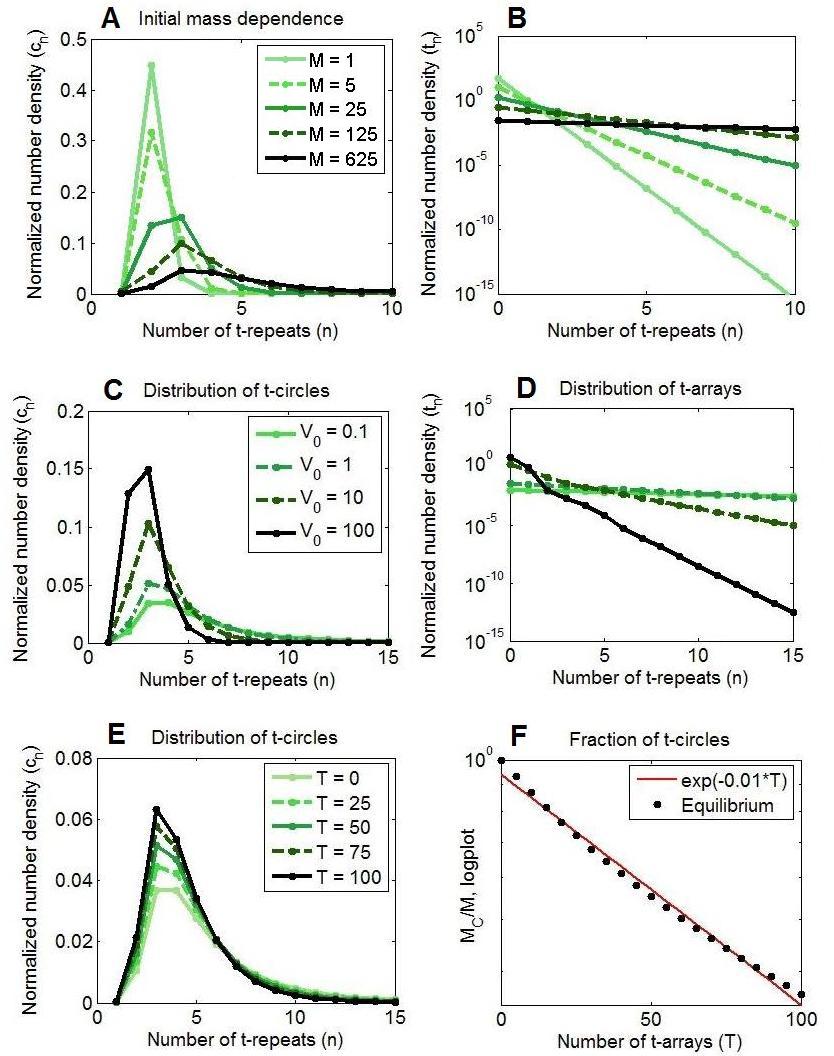
Figure 11: The dependence of the equilibrium t-circle size distribution in the CT-model of C. salmanticensis on the total number of t-repeats $M$ displayed on (A) a decimal and on (B) a logarithmic scale ($T=50$, $V_{0}=1\mu\text{m}^{3}$). The dependence of the equilibrium t-circle size distribution in the CT-model of C. salmanticensis on the sample volume $V_{0}$ (in units $1\mu\text{m}^{3}$) displayed on (C) a decimal and on (D) a logarithmic scale ($T=100$, $M=500$). (E) The dependence of the equilibrium t-circle size distribution in the CT-model of C. salmanticensis on the number $T$ of t-arrays ($V_{0}=1\mu\text{m}^{3}$, $M=500$). Distributions have a normalized mass for an easier comparison. (F) The dependence of the fraction $M_{C}/M$ of the t-repeats in t-circles on the number of t-arrays $T$ in the same model. With the increasing $T$ the ratio $M_{C}/M$ decreases exponentially.

Figure 11 AB displays a nonlinear dependence of the equilibrium of the t-circle size distribution in the CT-model for C. salmanticensis on the total number $M$ of t-repeats in the sample. A larger $M$ implies a shifted mean of the distribution towards longer t-circles. Both the distributions of t-circles and t-arrays have exponential tails.

Similarly, Fig. 11 CD shows a dependence of the CT-model equilibrium on the volume $V_{0}$ of the sample. Although the equilibrium formula in Eqs. 22 shows only a linear dependence on $V_{0}$, a different value of $V_{0}$ also effects the value of the parameter $b$ and thus has a nonlinear effect on the t-circle size distribution. An increasing sample volume shifts the distribution towards smaller circles as the number of the t-repeats in the t-circles decreases (with a conserved total number $M$ in the system).

Moreover, larger $T$ creates an opportunity for more t-repeats to be stored in t-arrays than in t-circles thus changing the proportion of the total mass in t-circles (see Fig. 11 EF). However, not only the proportion of the total mass in t-circles decreases with increasing $T$ but, consequently, the shape of the size distribution of t-circles adjusts as well (although not significantly). According to the numerical observations

$$M_{C}\approx Me^{-aT}\,,\qquad a>0\,.$$ (25)

We were not able to justify the approximation in Eq. 25 rigorously.

V Conclusions and Discussion

A hierarchy of mathematical models of alternative telomere length maintenance via recombination on the short time scale was constructed based on telomere biophysics. A good agreement of the model with experimentally measured size distributions of t-circles in yeast mitochondria was obtained across various yeast species. The robustness of the approach is demonstrated in ability to match the experimental data even on the level of the simplest C-model without fitting any artificial parameters. The predicted size distributions of t-circles and t-arrays in both C-model and CT-model are characterized by simple algebraic formulae that show a high importance of the values of the J-factor for the t-circle distributions. The size distributions of t-circles are the same for both models pointing out the scenario in which the dynamics of t-circles is not influenced by t-arrays, i.e., a possible universal mechanism of t-circle length maintenance independent of t-arrays. As the model system characterizes the recombination dynamics of linear and circular structures in general, these properties may be shared by various systems in applications.

In the rest of this section we discuss several distinct phenomena uncovered by our analysis that may be tested in the biological experiments and lead to an advance in understanding of telomere length maintenance. We also point out some of the limitations of the proposed model.

Excess mass. Our numerical simulations supported by rigorous mathematical analysis point out an interesting phenomenon of excess mass in the C-model responsible for creation of large t-circles that may be present in vivo under the condition of sufficiently large density of t-repeats. This mechanism can create extremely long t-circles if the cell division halts but cell keeps producing more t-repeats in mitochondria by the rolling circle mechanism. Whether this phenomenon is biologically relevant and responsible for the unusual t-circles observed in experiments (e.g., a $C_{10}$ t-circle in P. philodendri, or $C_{9}$ t-circles in C. metapsilosis and C. parapsilosis, see Fig. 2) is unclear and remains a subject of our further investigations.

Nonlinear response. The rigorous analysis and numerical simulations reveal an interesting feature that can be possibly exploited in a quantitative estimation of a detection rate of the experimental methods (as Southern blot hybridization combined with electron microscopy Tomaska et al. (2000) or quantitative PCR method). Indeed, the equilibrium of the system has a nonlinear response to the number of t-repeats in the sample. If one interprets the experimentally obtained data as relative quantities of measured species of different sizes, the model then identifies the total number of t-repeats in the sample by using the location and a relative size of the peak of the distributions of t-arrays and t-circles. It allows us to relate the experimental measurements to an approximate number of particular polymers in the sample regardless of the applied technique.

Long time scale. A lack of available dynamical experimental data (time series) motivates another key assumption of this study, a very short time scale on which the total number of t-repeats in constant. Nevertheless, the principal interest lies in the alternative mechanism of telomere length maintenance on a longer time scale that includes synthesis of t-repeats via rolling-circle mechanism, cell division, and subsequently the end-replication problem, and DNA degradation. Such a complex model may shed light on many important biological question as how many of t-repeats are transfered from a mother cell to a daughter cell, what types of telomeres are transfered, how the internal cellular clock influences the telomere maintenance, etc., but such a study requires additional quantitative data from new experiments.

Environmental factors. Extensive studies in biophysical literature identify dependences of individual factors in kinetic rates on environmental parameters as temperature, salinity, or pH. Variations of these parameters in experiments and the subsequent measurement of the telomere size distributions, together with the predictions of the model, can eventually both serve as a justification of the biophysical components and lead to the further factor-dependent enhancement of the model.

Single cell vs. cell population. A central assumption of this essay is homogeneity of the environment in the experimental sample. However, the samples are prepared from multiple cells/mitochondria and the resulting distribution corresponds to a sum of telomere size distributions in the individual cells/mitochondria. A nonlinear dependence of telomere size distributions on the total number of t-repeats, inhomogeneity of cells in the sample and asynchrony of their phases of cell cycles prohibit a more detailed analysis. To achieve a better agreement with experimental data and consequently a better understanding of the telomere length maintenance process in a single cell rather than in a cell population, single cell measurements need to be obtained experimentally or a model with age structured population of cells needs to be developed.

J-factor alternatives. We have presented our results for the particular choice of the values of the J-factor (Eqs. 11 and 13). However, other choices may be relevant: one may use older Shimada-Yamakawa model Shimada and Yamakawa (1984) or to account for recent results for short polymers Han et al. (2009); Vafabakhsh and Ha (2012). Moreover, modified circular J-factor introduced in Rippe (2001) may be considered as well. By this means the experimental measurements of telomere length distributions in yeast mtDNA may serve as an alternative to the direct tethered particle methods for J-factor estimation. Particularly interesting would be experimental studies of species that use ALT and have t-repeats of length 30–100 bp. Also, simultaneous measurement of t-array and t-repeat size distributions would increase the robustness of the model, particularly in connection with single cell measurements.

Appendix A Experimental Setup

The full description of experimental methods used to obtain t-circle size distributions can be found in Tomaska et al. (2000) including the details on yeast strains and DNAs used, DNA isolation, and preparation of mitochondria. T-circles isolated from purified mitochondria by alkaline lysis were relaxed with DNase I, and aliquots prepared for EM were directly adsorbed to thin carbon foils and rotary shadow cast with tungsten. The samples were subsequently imaged using electron microscopy and images were scanned and post-processed on a computer to adjust for high contrast. The length of the molecules was individually measured (see Griffith et al. (1999) for more details).

Appendix B Quasi-Steady State Approximation and Reduction to the CT-model

Time scale separation allows to reduce a reaction kinetics system by the means of the quasi-steady state approximation (QSSA) (Atkins, 1994; Eigen, 1974) However, the QSSA can often be misleading and the conditions for its validity need to be checked carefully. We refer the reader to works of Schnell and Maini (2000) and Flach and Schnell (2006) for examples of wrong use of the QSSA.

Segel (1988) and Segel and Slemrod (1989) were the first to point out the connection of the QSSA in the Michaelis-Menten enzyme kinetics to the mathematical problem of singular perturbation. They also derived the proper conditions necessary for the validity of the QSSA for simple enzyme kinetics. These techniques for irreversible enzyme kinetics were extended beyond the traditional QSSA by Schnell and Maini (2002, 2003) to cover the regimes where the QSSA fails (see also (Tzafriri and Edelman, 2007)). Further (formal) extensions of the QSSA and related techniques for the reversible enzyme kinetics and bimolecular reactions were derived by Tzafriri and Edelman (2004, 2005).

The existing theory allows to formulate conditions for the validity of the QSSA for the individual reactions (R4), (R5), and (R6) (see Fig. 1). For the three step reversible reactions (R1) and (R2) and the partially reversible three-step reaction (R3) it is possible to formally derive the conditions by using an approach analogous to (Tzafriri and Edelman, 2005). However, the theory is not applicable for the infinite system of reactions (R1)–(R6) with telomeric structures of arbitrary size because the time scales in the system are intertwined. Any rigorous result justifying the QSSA for the infinite system (R1)–(R6) would be a significant contribution to the theory of the QSSA as even for the system (R1)–(R6) of finite size (with limited maximal length of the telomeric structures) the right conditions for validity of the QSSA have not been yet established.

Nevertheless, our numerical simulations indicate the validity of the QSSA in the system (R1)–(R6) that allows to eliminate all the intermediate products of all sizes in the system schematically described on Fig. 1. Therefore we use the QSSA for the whole system (R1)–(R6) and replace the ordinary differential equations describing the temporal dynamics of populations of recombination complexes and end invasion complexes by the equilibrium conditions imposing algebraic laws for the populations of complexes. The simplified system referred to as the CT-model consist of the mass action kinetic reactions in Eqs. 15–17 with the kinetic rates given by

$$k^{CC}(C_{m},C_{n}) = k_{1}\cdot\frac{k_{3}k_{5}}{k_{2}k_{4}+k_{2}k_{5}+k_{3}k_{5}}\,,$$

$$k^{C}(C_{m},C_{n}) = k_{6}\cdot\frac{k_{2}k_{4}}{k_{2}k_{4}+k_{2}k_{5}+k_{3}k_{5}}\,,$$

$$k^{TC}(T_{m},C_{n}) = k_{7}\cdot\frac{k_{9}k_{11}}{k_{8}k_{10}+k_{8}k_{11}+k_{9}k_{11}}$$

$$+k_{21}\cdot\frac{k_{23}}{k_{22}+k_{23}}\,,$$

$$k^{T}(T_{m},C_{n}) = k_{12}\cdot\frac{k_{8}k_{10}}{k_{8}k_{10}+k_{8}k_{11}+k_{9}k_{11}}$$

$$+k_{18}\cdot\frac{k_{20}}{k_{19}+k_{20}}\,,$$

$$k^{TT}(T_{m},T_{n},T_{p}) = k_{13}\cdot\frac{k_{15}k_{17}}{k_{14}k_{16}+k_{14}k_{17}+k_{15}k_{17}}$$

$$+k_{24}\cdot\frac{k_{26}}{k_{25}+k_{26}}\,.$$

A straightforward calculation yields the simplified kinetic rates

$$k^{CC}(C_{m},C_{n}) = mn\hat{k}g_{1}\,,$$

$$k^{C}(C_{m},C_{n}) = (m+n)j(m,n)\hat{k}g_{1}\,,$$

$$k^{TC}(T_{m},C_{n}) = n(m+\alpha)\hat{k}g_{1}\,,$$

$$k^{T}(T_{m},C_{n}) = \left(mj(n)+\alpha j^{\ast}(n)\right)\hat{k}g_{1}\,,$$

$$k^{TT}(T_{m},T_{n},T_{p}) = \left(\min(m,n,k,m+n-p)+\alpha\right)\hat{k}g_{1}$$

that reduce after rescaling of time and an assumption $j(n)=j^{\ast}(n)$ to Eq. 18.

Appendix C Mathematical formulation of the CT-model and the C-model

The system of reaction kinetics in chemical reactions in Eqs. 15–17 can be mathematically formulated as two coupled sets of infinite number of ordinary differential equations in Eqs. 1–2. The system describes time evolution of the concentrations $c_{m}$ and $t_{n}$ of the populations $C_{n}$, $n>0$, and $T_{n}$, $n\geq 0$, respectively, in the sample solvent. The Gaussian circular J-factor satisfying the detailed balance condition in Eq. 13 allows for an explicit equilibrium solution of the system of Eq. 1–2 given by Eq. 3 The free positive parameter $b$ is uniquely determined by the total initial number of t-repeats $M$ in the sample. Note that while the t-circle size distribution is determined (up to a factor $n$) by the product of the J-factor with the decaying exponential, the t-arrays distribution is exponentially decaying with the same exponential rate.

The CT-model does not fit into any traditionally considered classes of systems of differential equations and we are not aware of any known general analytical results for the system of Eqs. 1–2. On the other hand, the reduced C-model formulated as an infinite system of Eqs. 4 that describes the evolution of the population $c_{m}$ of t-circles of size $m$ (full t-repeats) falls into a class of typically studied systems of ordinary differential equations — the coagulation fragmentation systems. The parameters $k_{m,n}^{C}$ and $k_{m,n}^{CC}$ are called the fragmentation and the coagulation kernel, respectively.

The theory of coagulation-fragmentation systems concerns rigorous mathematical studies of either discrete systems of the form 4 or their continuous counterparts that allow non-integer sized particles in which the vector $(c_{1},c_{2},\dots)$ is replaced by a nonnegative real function $c=c(m)$, $m\geq 0$, and the sums on the right hand of Eq. 4 are replaced by integrals. In general such systems describe the dynamics of cluster growth with applications in biology, material science, or atmospheric physics (see (Cañizo Rincón, 2006) for an extensive survey).

Since there is a large amount of literature on the subject we only provide here a short list of publications and recommend an interested reader to search for further references within. The mathematical treatment of the problem in Eq. 4 in the context of physical chemistry can be traced back to an influential paper of (Aizenman and Bak, 1979) and its predecessor (Bak and Bak, 1959) where a survey of older literature can be found. Aizenman and Bak (1979) studied constant interaction kernels and proved uniqueness of solutions of Eq. 4 and their convergence to an equilibrium. Later on, Ball and Carr (1990) studied various types of the discrete coagulation-fragmentation models for a wider class of additive kernels. Da Costa (1995) proved existence and uniqueness of density conserving solutions for models with strong fragmentation in the sense of Carr (1992). More recently, Fournier and Mischler (2004) generalized the asymptotic results to the case of strong fragmentation. Their analysis requires a relative smallness of the initial data $M=M_{C}$.

In (Carr, 2012) the system in Eq. 4 is considered with three different choices for coagulation and fragmentation kernels. First, in the case of constant J-factor, the kernels are given by

$$k_{m,i}^{C}=m+i,\qquad k_{m,i}^{CC}=mi.$$ (26)

In that case the kernel only accounts for the combinatorial part of the real biophysical t-circle interactions. In this simple case the system is exactly solvable by the means of Laplace transform and it is easy to establish that an arbitrary initial data converge (uniformly on finite sets) to the unique equilibrium given by

$$c_{m}=\frac{e^{-bm}}{m}\,,\qquad\quad b>0,$$ (27)

where the free positive parameter $b$ is uniquely determined by the initial data. Moreover, the distribution converges to the equilibrium exponentially in time.

Due to the fact that the circular J-factor satisfies the detailed balance condition in Eq. 13 the equilibria of the system can be explicitly expressed as

$$c_{m}=\frac{j(m)}{m}e^{-bm}\,,\qquad\quad b\geq 0,$$ (28)

providing a very good agreement with the experimental data. Carr mathematically analyzed the particular case of the J-factor of the Gaussian polymer model with $j(m)=m^{-3/2}$ (after a normalization, see Eq. 12). Then

$$k_{m,n}^{C}=\frac{(m+n)^{5/2}}{(mn)^{3/2}},\qquad k_{m,n}^{CC}=mn,$$ (29)

In that case the set of equilibria is given by

$$c_{m}=\frac{e^{-bm}}{m^{5/2}}\,,\quad\qquad b\geq 0,$$ (30)

and there is an equilibrium of the maximal (critical) finite mass

$$M_{\text{max}}=\sum_{m=1}^{\infty}m^{-3/2}$$

(we set $V_{0}=1$ here for simplicity). Then all the solutions with the initial mass smaller than $M_{\text{max}}$ converge (uniformly on finite sets) to the appropriate equilibrium while the solutions with the initial mass larger or equal than $M_{\text{max}}$ converge (pointwise) to the equilibrium in Eq. 30 with $b=0$, and the excess mass is moving to higher and higher modes indicating weak convergence of the solution to the equilibrium of the critical mass in an appropriate functional space. Note that the scaling of the critical size distributions in Eq. 30 (for $b=0$) is the same as in (Ben-Naim and Krapivsky, 2011, Eq. 7) illustrating the generic nature of the phenomenon. Carr (2012) also considered more general case that accounts for size-dependent diffusion of the telomeres but the problem due to the change of the structure of the reaction rates posed a difficult unsolved mathematical problem.

An interesting feature of the CT-model (Eqs. 1–2) under the assumption of the circular J-factor with the detailed balance condition is that the algebraic form of its equilibrium given by Eq. 22 is in agreement with the equilibrium (Eq. 28) of the reduced C-model. The general reason for this fact is the compatibility of the kinetic reactions described by Eq. 15–17 connected to preservation of the mass (the number of t-repeats) in each individual reaction. However, if the circular J-factor is modeled using the theory of Rippe (2001), the equilibrium conditions forced by individual reaction in Eq. 15–17 are not compatible and there is no such simple formula for the equilibrium of the system.

Biophysical parameters	Value
Typical length of a basepair	$\xi=0.34$ nm (width 2 nm) (Moran et al., 2010)
Typical yeast cell size (S. cerevisiae)	$10\text{$\mu$m}$ (diameter), 20–160 $\text{$\mu$m}^{3}$ (volume) (Moran et al., 2010)
Estimated number of mtDNA copies in a haploid yeast cell (S. cerevisiae)	20-50 (10-20% of total DNA) (Williamson and Fennell, 1979)
Cell cycle time budding yeast	70–140 min (Moran et al., 2010)
Mitochondrial genome size, telomeric tandem repeat length C. salmanticensis	$25\,718+(m+n)\times 104$ bp (Nosek et al., 1995; Tomaska et al., 2000; Valach et al., 2011)
Mitochondrial genome size, telomeric tandem repeat length P. philodendri	$26\,487+(m+n)\times 288$ bp (Nosek et al., 1995)
Mitochondrial genome size, telomeric tandem repeat length C. metapsilosis	$23\,062+(m+n)\times 620$ bp (Kosa et al., 2006)
Mitochondrial genome size, telomeric tandem repeat length C. parapsilosis	$30\,923+(m+n)\times 738$ bp (Nosek et al., 1995)
Length of the single-stranded 5′ overhang	$110\times\xi$ nm (110 nt) (Nosek et al., 1995)
Estimated typical length of a hotspot	$l_{\text{HS}}=10$ bp
Bending and torsional persistence length of DNA as a homogeneous polymer	$\ell_{p}=50$ nm (Wilson et al., 2010)
Boltzmann constant	$k_{B}=1.3806503\times 10^{-23}\text{m}^{2}\text{kg}/\text{s}^{2}\text{K}$
Absolute temperature	$T_{\text{a}}=273.15K$
Solvent viscosity	$\hat{\nu}=1.2\times 10^{-9}\text{kg}/\text{$\mu$m}\,\text{s}$ (Robertson et al., 2006)

Table 1: Biophysical parameters

References

- Lapidus et al. (2000) L. J. Lapidus, W. A. Eaton, and J. Hofrichter, Proc. Natl. Acad. Sci. USA 97, 7220 (2000)
- Langowski and Schiessel (2006) J. Langowski and H. Schiessel, “Chromatin simulations. from DNA to chromatin fibers,” in Computational studies of RNA and DNA, Šponer, J. and Lankaš, F. (Eds.), Challanges and advances in computational chemistry and physics, Vol. 2 (Springer, 2006) pp. 605–634
- Perico and Beggiato (1990) A. Perico and M. Beggiato, Macromolecules 23, 797 (1990)
- Wittmer et al. (2000) J. P. Wittmer, P. van der Schoot, A. Milchev, and J. L. Barrat, J. Chem. Phys. 113, 6992 (2000)
- Ben-Naim and Krapivsky (2011) E. Ben-Naim and P. L. Krapivsky, Phys. Rev. E 83, 061102 (2011)
- McEachern et al. (2000) M. McEachern, A. Krauskopf, and E. Blackburn, Annu. Rev. Genet. 34, 331 (2000)
- Arino et al. (1995) O. Arino, M. Kimmel, and G. F. Webb, J. Theor. Biol. 177, 45 (1995)
- Levy et al. (1992) M. Levy, R. Allsopp, A. Futcher, C. Greider, and C. Harley, J. Mol. Biol. 225, 951 (1992)
- De Boer and Noest (1998) R. J. De Boer and A. J. Noest, J. Immunol. 160, 5832 (1998)
- Rubelj and Vondraček (1999) I. Rubelj and Z. Vondraček, J. Theor. Biol. 197, 425 (1999)
- Arkus (2005) N. Arkus, J. Theor. Biol. 235, 13 (2005)
- Olofsson and Bertuch (2010) P. Olofsson and A. Bertuch, J. Theor. Biol. 263, 353 (2010)
- Rodriguez-Brenes and Peskin (2010) I. Rodriguez-Brenes and C. Peskin, Proc. Natl. Acad. Sci. USA 107, 5387 (2010)
- Dao Duc and Holcman (2013) K. Dao Duc and D. Holcman, Phys. Rev. Lett. 111, 228104 (2013)
- Nosek et al. (1995) J. Nosek, N. Dinouël, L. Kovac, and H. Fukuhara, Mol. Gen. Genet. 247, 61 (1995)
- Tomaska et al. (2004) L. Tomaska, M. McEachern, and J. Nosek, FEBS Lett. 567, 142 (2004)
- Rycovska et al. (2004) A. Rycovska, M. Valach, L. Tomaska, M. Bolotin-Fukuhara, and J. Nosek, Microbiology 150, 1571 (2004)
- Nosek et al. (2005) J. Nosek, A. Rycovska, A. Makhov, J. Griffith, and L. Tomaska, J. Biol. Chem. 280, 10840 (2005)
- Tomaska et al. (2000) L. Tomaska, J. Nosek, A. Makhov, A. Pastorakova, and J. Griffith, Nucl. Acids Res. 28, 4479 (2000)
- Kosa et al. (2006) P. Kosa, M. Valach, L. Tomaska, K. Wolfe, and J. Nosek, Nucl. Acids Res. 34, 2472 (2006)
- Olovnikov (1971) A. Olovnikov, Dokl. Akad. Nauk SSSR 201, 1496 (1971)
- Watson (1972) J. D. Watson, Nat. New Biol. 239, 197 (1972)
- Cesare and Reddel (2010) A. Cesare and R. Reddel, Nat. Rev. Genet 11, 319 (2010)
- Conomos et al. (2013) D. Conomos, H. A. Pickett, and R. R. Reddel, Front. Oncol. (2013), doi: 10.3389/fonc.2013.00027
- Aizenman and Bak (1979) M. Aizenman and T. A. Bak, Comm. Math. Phys. 65, 203 (1979)
- Ball and Carr (1990) J. M. Ball and J. Carr, J. Stat. Phys. 61, 203 (1990)
- Greider and Blackburn (1985) C. Greider and E. Blackburn, Cell 43, 405 (1985)
- Greider and Blackburn (1987) C. Greider and E. Blackburn, Cell 51, 887 (1987)
- Lundblad (2002) V. Lundblad, Oncogene 21, 522 (2002)
- Pardue and DeBaryshe (2003) M. Pardue and P. DeBaryshe, Annu. Rev. Genet. 37, 485 (2003)
- Griffith et al. (1999) J. Griffith, L. Comeau, S. Rosenfield, R. Stansel, A. Bianchi, H. Moss, and T. de Lange, Cell 97, 503 (1999)
- Nakamura et al. (1998) T. Nakamura, J. Cooper, and T. Cech, Science 282, 493 (1998)
- Qin and Cohen (2002) Z. Qin and S. Cohen, Mol. Microbiol. 45, 785 (2002)
- Jain et al. (2010) D. Jain, A. Hebden, T. Nakamura, K. Miller, and J. Cooper, Nature 467, 223 (2010)
- McEachern and Blackburn (1996) M. McEachern and E. Blackburn, Genes Dev. 10, 1882 (1996)
- Teng and Zakian (1999) S. Teng and V. Zakian, Mol. Cell Biol. 19, 8083 (1999)
- Teng et al. (2000) S. Teng, J. Chang, B. McCowan, and V. Zakian, Mol. Cell 6, 947 (2000)NoStop
- Biessmann and Mason (1997) H. Biessmann and J. Mason, Chromosoma 106, 63 (1997)
- Dunham et al. (2000) M. Dunham, A. Neumann, C. Fasching, and R. Reddel, Nature Genet. 26, 447 (2000)
- Niida et al. (2000) H. Niida, Y. Shinkai, M. Hande, T. Matsumoto, S. Takehara, M. Tachibana, M. Oshimura, P. Lansdorp, and Y. Furuichi, Mol. Cell Biol. 20, 4115 (2000)NoStop
- Tomaska et al. (2009) L. Tomaska, J. Nosek, J. Kramara, and J. Griffith, Nat. Struct. Mol. Biol. 16, 1010 (2009)
- Tomaska et al. (2002) L. Tomaska, A. Makhov, J. Griffith, and J. Nosek, Mitochondrion 1, 455 (2002)
- Oganesian and Karlseder (2011) L. Oganesian and J. Karlseder, Mol. Cell 42, 224 (2011)
- Note (1) An assumption enabling a description of the dynamics in a form of system of ordinary differential equations rather than physically more realistic partial differential equations
- Note (2) In general, more hotspots within one t-repeat can exist and their number can be treated as a parameter of the model that can be quantitatively estimated
- Jackson (2006) M. B. Jackson, Molecular and Cellular Biophysics (Cambridge University Press, 2006)
- Robertson et al. (2006) R. Robertson, S. Laib, and D. Smith, Proc. Natl. Acad. Sci. USA. 103, 7310 (2006)
- Flory (1953) P. J. Flory, Principles of Polymer Chemistry (Cornell Univ. Press, Ithaca, New York, 1953)
- Jacobson and Stockmayer (1950) H. Jacobson and W. H. Stockmayer, J. Chem. Phys. 18, 1600 (1950)
- Phillips et al. (2009) R. Phillips, J. Kondev, J. Theriot, N. Orme, and H. Garcia, Physical biology of the cell (Garland Science, 2009)
- Noyes (1961) R. M. Noyes, Prog. React. Kinet. 1, 129 (1961)
- Towles et al. (2009) K. B. Towles, J. F. Beausang, H. G. Garcia, R. Phillips, and P. C. Nelson, Phys. Biol. 6, 025001 (2009)
- Allemand et al. (2006) J.-F. Allemand, S. Cocco, N. Douarche, and G. Lia, Eur. Phys. J. E Soft Matter 19, 293 (2006)
- Kratky and Porod (1949) O. Kratky and G. Porod, Rec. Trav. Chim. Pays-Bas 68, 1106 (1949)
- Shore et al. (1981) D. Shore, J. Langowski, and R. L. Baldwin, Biochemistry 78, 4833 (1981)
- Shimada and Yamakawa (1984) J. Shimada and H. Yamakawa, Macromolecules 17, 689 (1984)
- Ringrose et al. (1999) L. Ringrose, S. Chabanis, P. O. Angrand, C. Woodroofe, and A. F. Stewart, EMBO J. 18, 6630 (1999)
- Rippe et al. (1995) K. Rippe, P. H. von Hippel, and J. Langowski, Trends Biochem. Sci. 20, 500 (1995)
- Vologodskii (2009) A. Vologodskii, “Statistical-mechanical analysis of enzymatic topological transformations in DNA molecules, benham, c. j. et al. (eds.),” in Mathematics of DNA Structure, Function and Interactions, IMA Vol. in Math. and Appl. 150 (Springer, 2009)
- Bloomfield (1974) V. Bloomfield, Physical chemistry of nucleic acids (Harper & Row, 1974)
- Rippe (2001) K. Rippe, Trends Biochem. Sci. 26, 733 (2001)
- Podtelezhnikov et al. (2000) A. A. Podtelezhnikov, C. Mao, N. C. Seeman, and A. Vologodskii, Biophys. J. 79, 2692 (2000)
- Hanke and Metzler (2003) A. Hanke and R. Metzler, Biophys. J. 85, 167 (2003)
- Han et al. (2009) L. Han, H. G. Garcia, S. Blumberg, K. B. Towles, J. F. Beausang, P. C. Nelson, and R. Phillips, PLoS ONE 4, e5621 (2009)
- Saiz and Vilar (2006) L. Saiz and J. M. Vilar, Curr. Opin. Struc. Biol. 16, 344 (2006)
- Vafabakhsh and Ha (2012) R. Vafabakhsh and T. Ha, Science 337, 1097 (2012)
- Nelson (2012) P. C. Nelson, Science 337, 1045 (2012)
- Sanchez et al. (2011) A. Sanchez, H. G. Garcia, D. Jones, R. Phillips, and J. Kondev, PLoS Comp. Biol. 7, e1001100 (2011)
- Note (3) The coefficient 2 in corresponding Eq. 10 in Shore et al. (1981) accounts for two indistinguishable ends of the linear polymers while here the interacting hotspots are distinguishable.
- Atkins (1994) P. Atkins, Physical Chemistry (Academic Press, New York, 1994) pp. 927–935
- Eigen (1974) M. Eigen, “Diffusion control in biochemical reactions,” in Quantum Statistical Mechanics in the Natural Sciences, Kurusungolu, B.et al. (Eds.) (Plenum, New York, 1974) pp. 37–61
- Segel and Slemrod (1989) L. Segel and M. Slemrod, SIAM Rev. 31, 446 (1989)
- Schnell and Maini (2003) S. Schnell and P. K. Maini, Comm. Theor. Biol. 8, 169 (2003)
- Tzafriri and Edelman (2005) A. R. Tzafriri and E. R. Edelman, J. Theor. Biol. 233, 343 (2005)
- Bak and Bak (1959) T. A. Bak and K. Bak, Acta Chem. Scand. 13, 1997 (1959)
- Da Costa (1995) F. P. Da Costa, J. Math. Anal. Appl. 192, 892 (1995)
- Note (4) A further mathematical analysis reveals that the convergence to the equilibrium in the system is exponential
- Carr (2012) J. Carr, written communication (2012)
- Moran et al. (2010) U. Moran, R. Phillips, and R. Milo, Cell 141, 1262 (2010)
- Williamson and Fennell (1979) D. H. Williamson and D. J. Fennell, Methods Enzymol. 56, 728 (1979)
- Valach et al. (2011) M. Valach, Z. Farkas, D. Fricova, J. Kovac, B. Brejova, T. Vinar, I. Pfeiffer, J. Kucsera, L. Tomaska, B. F. Lang, et al., Nucl. Acids Res. 39, 4202 (2011)
- Wilson et al. (2010) D. P. Wilson, A. V. Tkachenko, and J. C. Meiners, Europhys. Let. 89, 58005 (2010)
- Schnell and Maini (2000) S. Schnell and P. Maini, Bull. of Math. Biol. 62, 483 (2000)
- Flach and Schnell (2006) E. H. Flach and S. Schnell, Syst. Biol. 153, 187 (2006)
- Segel (1988) L. A. Segel, Bull. Math. Biol. 50, 579 (1988)
- Schnell and Maini (2002) S. Schnell and P. K. Maini, Math. Comput. Model. 35, 137 (2002)
- Tzafriri and Edelman (2007) A. R. Tzafriri and E. R. Edelman, J. Theor. Biol. 245, 737 (2007)
- Tzafriri and Edelman (2004) A. R. Tzafriri and E. R. Edelman, J. Theor. Biol. 226, 303 (2004)
- Cañizo Rincón (2006) J. A. Cañizo Rincón, Some problems related to the study of interaction kernels: coagulation, fragmentation and diffusion in kinetic and quantum equations, Ph.D. thesis, Universidad de Granda (2006)
- Carr (1992) J. Carr, Proc. Roy. Soc. Edinburgh A 121, 231 (1992)
- Fournier and Mischler (2004) N. Fournier and S. Mischler, Proc. Roy. Soc. London A 460, 2477 (2004)
- Carr (2012) J. Carr, written communication (2012)