The longitudinal structure function $F_{L}$ from the charm structure function $F_{2}^{c}$

Abstract

We predict the effect of the charm structure function on the longitudinal structure function at small $x$. In NLO analysis we find that the hard Pomeron behavior gives a good description of $F_{L}$ and $F_{k}^{c}(k=2,L)$ at small $x$ values. We conclude that a direct relation between $F_{L}{\propto}\hskip 2.84544ptF_{2}^{c}$ would provide useful information on how to measurement longitudinal structure function at high $Q^{2}$ values. Having checked that this model gives a good description of the data, when compared with other models.

In the LO (leading order), authors in Ref.[1] have suggested an approximation relation between the gluon density and the longitudinal structure function $F_{L}$, which demonstrates the close relation between the longitudinal structure function and the gluon density. Therefore the longitudinal structure function is a very clean probe of the small $x$ gluon distribution. We specifically consider the next- to- leading- order (NLO) corrections to the longitudinal structure function $F_{L}$, projected from the hadronic tensor by combination of the metric and the spacelike momentum transferred by the virtual photon $(g_{\mu\nu}-q_{\mu}q_{\nu}/q^{2})$. In the next- to -leading order the longitudinal structure function is proportional to hadronic tensor as follows:

$$F_{L}(x,Q^{2})/x=\frac{8x^{2}}{Q^{2}}p_{\mu}p_{\nu}W_{\mu\nu}(x,Q^{2}),$$ (1)

where $p^{\mu}(p^{\nu})$ is the hadron momentum and $W^{\mu\nu}$ is the hadronic tensor. In this relation we neglecting the hadron mass.

The basic hypothesis is that the total cross section of a hadronic process can be written as the sum of the contributions of each parton type (quarks, antiquarks, and gluons) carrying a fraction of the hadronic total momentum. In the case of deep- inelastic- scattering it reads:

$$d\sigma_{H}(p)=\sum_{i}{\int}dyd\hat{\sigma}_{i}(yp)\Pi_{i}^{0}(y),$$ (2)

where $d\hat{\sigma}_{i}$ is the cross section corresponding to the parton $i$ and $\Pi_{i}^{0}(y)$ is the probability of finding this parton in the hadron target with the momentum fraction $y$. Now, taking into account the kinematical constrains one gets the relation between the hadronic and the partonic structure functions:

$$f_{j}(x,Q^{2}) = \sum_{i}{\int}_{x}^{1}\frac{dy}{y}\textsf{f}_{j}(\frac{x}{y},Q^{2})\Pi_{i}^{0}(y)$$

$$=\sum_{i}\textsf{f}_{j}{\otimes}\Pi_{i}^{0}(y)\hskip 14.22636pt,j=2,L,$$

where $\textsf{f}_{j}(x,Q^{2})=F_{j}(x,Q^{2})/x$ and the symbol ${\otimes}$ denotes convolution according to the usual prescription. Equation (3) expresses the hadronic structure functions as the convolution of the partonic structure function, which are calculable in perturbation theory, and the probability of finding a parton in the hadron which is a nonperturbative function. So, in correspondence with Eq.(3) one can write Eq.(1) for the gluon density dominated at low $x$ values by follows:

$$F^{g}_{L}/x{=}\frac{\alpha_{s}}{4\pi}[\textsf{f}_{L,G}^{(1)}{\otimes}g^{0}]+(\frac{\alpha_{s}}{4\pi})^{2}[\textsf{f}_{L,G}^{(2)}{\otimes}g^{0}],$$ (4)

where $\textsf{f}_{L,G}^{(1)}$ and $\textsf{f}_{L,G}^{(2)}$ are the LO and NLO partonic longitudinal structure function corresponding to gluons, respectively [2-3]. We present the expressions, after full agreement has been achieved, in the form of kernels $K^{G}$ which give NLO- $F_{L}$ upon convolution with the gluon distribution:

$$F^{g}_{L}(x,Q^{2}) = K^{G}(\frac{x}{y},Q^{2}){\otimes}G(y,Q^{2})$$

$$=\int_{x}^{1}\frac{dy}{y}K^{G}(\frac{x}{y},Q^{2})G(y,Q^{2}),$$

where $K^{G}(x,Q^{2})$ is the DIS coefficient function and the explicit form of it^,s appears in the Appendix.
Exploiting the small $x$ asymptotic behavior of the gluon distribution [4] into the symbolic form,

$$G(x,Q^{2})|_{x{\rightarrow}0}{\rightarrow}x^{-\delta},$$ (6)

where the exponent of the gluon distribution is found to be either $\delta{\approx}0$ or $\delta{\approx}0.5$. The first value corresponds to the soft pomeron intercept and the second value to the hard (Lipatov) pomeron intercept.
Using Eq.6 in 5, the integration of the gluon kernel over $z=\frac{x}{y}$ and finally summing over the gluon distribution function $G(x,Q^{2})$ yields:

$$F^{g}_{L}(x,Q^{2}) = G(x,Q^{2})[K^{G}(1-z,Q^{2}){\otimes}(1-z)^{\delta}]$$

$$=G(x,Q^{2})\int_{0}^{1-x}K^{G}(1-z,Q^{2})(1-z)^{\delta}dz.$$

The objective this paper is the determination of $F_{L}$ with respect to the $F_{2}^{c}$. In this context it is interesting to recall that $F_{L}$ and $F_{k}^{c}(k=2,L)$ contain an appreciable part directly sensitive to the gluon density at small $x$. In addition, we systematically analyze the relation between this approach and charm structure functions $F_{k}^{c}(k=2,L)$, as these results are independent of the exact gluon kinematics .

Let us first discuss charm production, and some phenomenological aspects of the observable relevant to the charm structure functions for the experimental data at HERA, and its contribution to the longitudinal structure function $F_{L}$. In the case of heavy quark production, we can have condition that the heavy quarks produced from the boson- gluon fusion (BGF) via $\gamma^{*}g{\rightarrow}c\overline{c}$. That is, in PQCD calculations the production of heavy quarks at HERA proceeds dominantly via the direct BGF where the photon interacts with a gluon in the proton by the exchange of a heavy quark pair [5-12]. In NLO perturbative QCD, the charm structure functions $F_{k}^{c}(k=2,L)$ are given by [13]

$$F_{k}^{c}(x,Q^{2}) = C_{g,k}^{c}(\frac{x}{y},Q^{2}){\otimes}G(y,Q^{2})$$

$$=2xe_{c}^{2}\frac{\alpha_{s}(\mu^{2})}{2\pi}\int_{ax}^{1}\frac{dy}{y}C_{g,k}^{c}(\frac{x}{y},\zeta)g(y,\mu^{2}),$$

where $a=1+4\zeta(\zeta{\equiv}\frac{m_{c}^{2}}{Q^{2}})$ and the renormalization scale $\mu$ is assumed to be either $\mu^{2}=4m_{c}^{2}$ or $\mu^{2}=4m_{c}^{2}+Q^{2}$. Here $C^{c}_{g,k}$ is the charm coefficient function in LO and NLO analysis as

$$C_{k,g}(z,\zeta) {\rightarrow} C^{0}_{k,g}(z,\zeta)+a_{s}(\mu^{2})[C_{k,g}^{1}(z,\zeta)$$

$$+\overline{C}_{k,g}^{1}(z,\zeta)ln\frac{\mu^{2}}{m_{c}^{2}}],$$

where $a_{s}(\mu^{2})=\frac{\alpha_{s}(\mu^{2})}{4\pi}$ and in the NLO analysis

$$\alpha_{s}(\mu^{2})=\frac{4{\pi}}{\beta_{0}ln(\mu^{2}/\Lambda^{2})}-\frac{4\pi\beta_{1}}{\beta_{0}^{3}}\frac{lnln(\mu^{2}/\Lambda^{2})}{ln(\mu^{2}/\Lambda^{2})}$$ (10)

with $\beta_{0}=11-\frac{2}{3}n_{f},\beta_{1}=102-\frac{38}{3}n_{f}$ ($n_{f}$ is the number of active flavours), $\zeta{\equiv}\frac{m_{c}^{2}}{Q^{2}}$ and $\mu$ is the renormalization scale.
In the LO analysis, the coefficient functions BGF can be found [14-16], as

$$C^{0}_{g,2}(z,\zeta) = \frac{1}{2}([z^{2}+(1-z)^{2}+4z\zeta(1-3z)-8{\zeta^{2}}z^{2}]$$ (11)

$${\times}ln\frac{1+\beta}{1-\beta}+{\beta}[-1+8z(1-z)$$

$$-4z{\zeta}(1-z)]),$$

and

$$C^{0}_{g,L}(z,\zeta)=-4z^{2}{\zeta}ln\frac{1+\beta}{1-\beta}+2{\beta}z(1-z),$$ (12)

where $\beta^{2}=1-\frac{4z\zeta}{1-z}$. At NLO, $O(\alpha_{em}\alpha_{s}^{2})$, the contribution of the photon- gluon component is usually presented in terms of the coefficient functions $C_{k,g}^{1},\overline{C}_{k,g}^{1}$. Using the fact that the virtual photon- quark(antiquark) fusion subprocess can be neglected, because their contributions to the heavy-quark leptoproduction vanish at LO and are small at NLO. In a wide kinematic range, the contributions to the charm structure functions in NLO are not positive due to mass factorization. Therefore the charm structure functions are dependence to the gluonic observable in LO and NLO. The NLO coefficient functions are only available as computer codes[13,17]. But in the high- energy regime ($\zeta<<1$) we can used the compact form of these coefficients according to the Refs.[18,19].

Using Eq.6, We recall the relation between the charm structure functions and the gluon distribution function at small $x$ and the limit $\mu^{2}{\rightarrow}Q^{2}$, we obtain the effective formula for the charm structure functions as

$$F_{k}^{c}(x,Q^{2}) = G(x,Q^{2})[C_{g,k}^{c}(1-z,Q^{2}){\otimes}(1-z)^{\delta}]$$ (13)

$$=2e_{c}^{2}\frac{\alpha_{s}(\mu^{2})}{2\pi}G(x,Q^{2}){\times}$$

$$\int_{1-\frac{1}{a}}^{1-x}C_{g,k}^{c}(1-z,\zeta)(1-z)^{\lambda_{g}}dz,$$

here $C_{g,k}^{c}$ is defined by Eq.9. The main input to the Eqs.7 and 13 is the gluon distribution $G(x,Q^{2})$. These equations give predictions for the structure functions as a function of the gluon distribution. Inserting Eq.7 in Eq.13, we obtain our master formula for the charm structure functions into the longitudinal proton structure function, as

$$F_{k}^{c}(x,Q^{2})=\frac{[C_{g,k}^{c}(1-z,Q^{2}){\otimes}(1-z)^{\delta}]}{[K^{G}(1-z,Q^{2}){\otimes}(1-z)^{\delta}]}F^{g}_{L}(x,Q^{2}).$$ (14)

In fact, this equation which is independent of the gluon distribution function , is very useful for practical applications. In this equation we used the solutions of the NLO BGF analysis ($C_{g,k}^{c}$), NLO kernels ($K^{G}$) and considered $\delta$ as a hard (Lipatov) Pomeron exponent. We observe that the longitudinal structure function measurement at DESY $ep$ collider HERA will be able to make a reasonably precise measurement of the charm structure functions at low $x$ values.

Having checked that this formula reproduces satisfactory the existing the longitudinal proton structure function into the charm structure function at high $Q^{2}$ values. One finds the following final form for the longitudinal structure function, as

$$F^{g}_{L}(x,Q^{2})=\frac{[K^{G}(1-z,Q^{2}){\otimes}(1-z)^{\delta}]}{[C_{g,k}^{c}(1-z,Q^{2}){\otimes}(1-z)^{\delta}]}F_{2}^{c}(x,Q^{2}).$$ (15)

Recently, H1 Collaboration measures the longitudinal proton structure function [11] and charm structure function [12], as data for the longitudinal proton structure function are existing only at $Q^{2}{\leq}45GeV^{2}$. Therefore, when analysis the charm structure function, it is particularly important to obtain our prediction according to Eq.15 for the longitudinal structure function at $Q^{2}{>}45GeV^{2}$, rather than to low $Q^{2}$ values of $F_{L}(x,Q^{2})$.

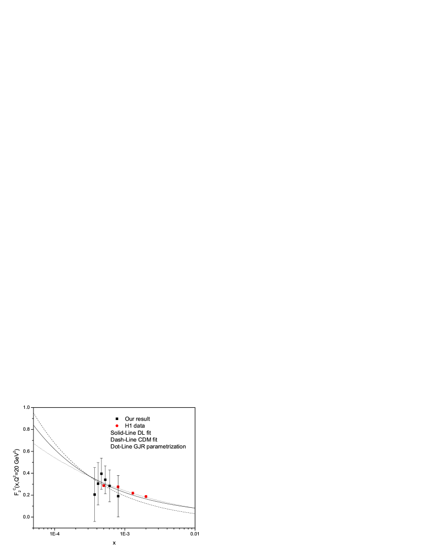
Figure 1: The charm component of the structure function at $Q^{2}=20GeV^{2}$ according to the longitudinal structure function input [11]. Our results accompanied with the errors due to the renormalization scales, compared to H1 data [12], and also A.Donnachie- P.V.Landshoff (DL) model [7], GJR parameterization [20] and color dipole model (CDM) [21] .

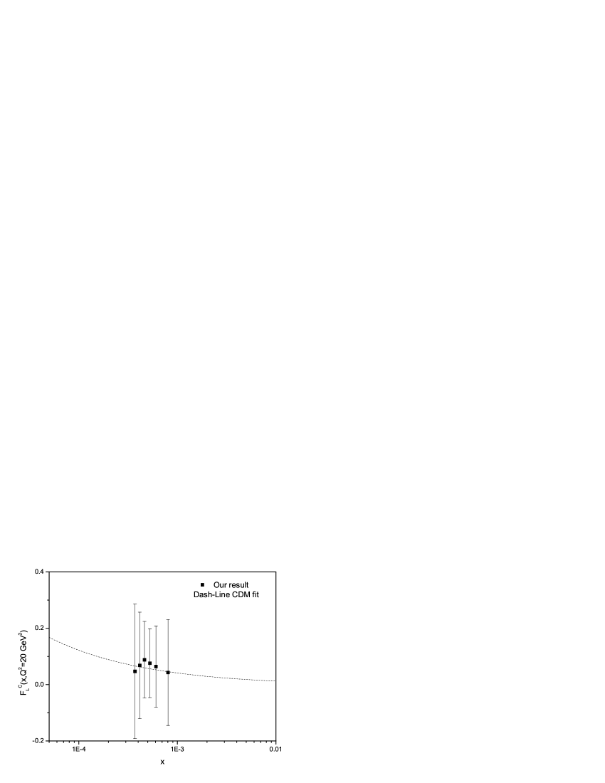
Figure 2: The charm component of the longitudinal structure function at $Q^{2}=20GeV^{2}$ according to the longitudinal structure function input [11]. Our results accompanied with the errors due to the renormalization scales, compared only to the color dipole model (CDM) [21].

We start our numerical analysis by comparing the calculations of the structure functions with the experimental data and other models. To be precise, we use the formulae (14,15) with $\Lambda=0.224GeV$, $m_{c}=1.25GeV$ and $\delta{\simeq}0.5$. Now extract $F_{k}^{c\overline{c}}$ from the H1 measurements of the longitudinal proton structure function [11] in Eq.14. Our NLO results for the charm structure functions $F_{k}^{{}^{c}}(x,Q^{2})(k=2\hskip 2.84544pt\&\hskip 2.84544ptL)$ are presented in Table 1 for each bin in $Q^{2}$ and $x$. In Table 2 we show our results for the charm structure functions at $Q^{2}=20GeV^{2}$ for various values of $x$. In Figs.1 and 2 we show the calculations obtained for the charm structure functions using this approach with the longitudinal structure function data. The charm structure functions are plotted as a function of $x$ at $Q^{2}=20GeV^{2}$. The data shown in Fig.1 are from H1 [12] experiment. In Figs.1 and 2 we compared our results for the $F_{2}^{c}$ and $F_{L}^{c}$ with DL fit [7], GJR parameterization [20] and color-dipole model (CDM) [21], respectively. The agreement between the experimental data and other models with our calculations is good.

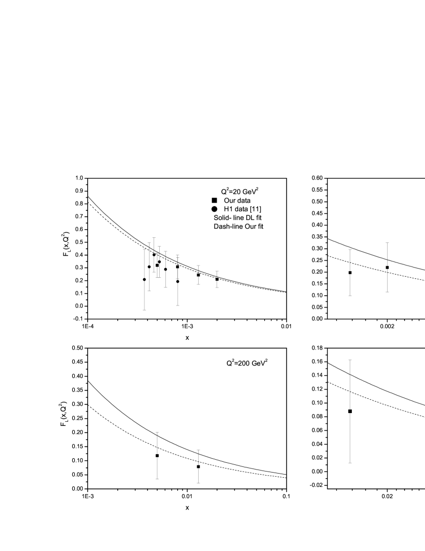
Figure 3: Predictions for $F_{L}(x,Q^{2})$ at NLO, from the charm structure function data [12] at $Q^{2}$ values of 20, 60, 200 and 650 $GeV^{2}$. Our results accompanied with the errors due to the renormalization scales, compared to the DL model [22].

We stress though the importance of the existent data in the evaluation of the longitudinal structure function at high $Q^{2}$ values. In Table 3 we predict the longitudinal structure function $F_{L}(x,Q^{2})$ with respect to the H1 measurements of the charm structure function $F_{2}^{{}^{c}}(x,Q^{2})$ [12] in Eq.15 at low and high $Q^{2}$ values. Our NLO results for $Q^{2}=20,60,200$ and $650GeV^{2}$ are presented. We observe that theoretical uncertainty related to the freedom in the choice of the renormalization scales $\mu^{2}=4m^{2}_{c}$ and $\mu^{2}=4m^{2}_{c}+Q^{2}$ as accompanied to the total errors of the measurements data at the quadrature procedure. In Fig.3, we show the prediction of Eq.15 for the longitudinal structure function. We compare our results for $F_{L}$ with the H1 [11] data and DL model [22]. As can be seen, the values of the longitudinal structure function increase as $x$ decreases. This is because the hard- Pomeron exchange defined by DL model is expected to hold in the small- $x$ limit.

In summary, we have presented Eq.15 for the extraction of the longitudinal structure function $F_{L}$ at low $x$ and high $Q^{2}$ values from the charm structure function $F_{2}^{c}$. This approximation relation provide the possibility the non-direct determination $F_{L}$. This is important since the direct extraction of $F_{L}$ from experimental data is a cumbersome procedure. We have found that the charm structure function gave us the longitudinal structure function that agrees well with the phenomenological fit. Having checked that this approach gives a good description of the data, we have used it to predict $F_{L}$ and $F_{2}^{c}$ to be measured in collisions.

.1 Appendix

The explicit form of the gluon kernel is given by the following from:

$$K^{G}(\frac{x}{y},Q^{2}) = \frac{\alpha_{s}}{4\pi}[8(x/y)^{2}(1-x/y)][\sum_{i=1}^{N_{f}}e_{i}^{2}]+(\frac{\alpha_{s}}{4\pi})^{2}[\sum_{i=1}^{N_{f}}e_{i}^{2}]16C_{A}(x/y)^{2}(+4dilog(1-x/y)$$

$$-2(1-x/y)ln(x/y)ln(1-x/y)+2(1+x/y)dilog(1+x/y)+3ln(x/y)^{2}+2(x/y-2)\pi^{2}/6$$

$$+(1-x/y)ln(1-x/y)^{2}+2(1+x/y)ln(x/y)ln(1+x/y)+\frac{(24+192x/y-317(x/y)^{2})}{24(x/y)}ln(x/y)$$

$$+\frac{(1-3x/y-27(x/y)^{2}+29(x/y)^{3})}{3(x/y)^{2}}ln(1-x/y)+\frac{(-8+24x/y+510(x/y)^{2}-517(x/y)^{3})}{72(x/y)^{2}}$$

$$-16C_{F}(x/y)^{2}(\frac{5+12(x/y)^{2}}{30}ln(x/y)^{2}-(1-x/y)ln(1-x/y)+\frac{-2+10(x/y)^{3}-12(x/y)^{5})}{15(x/y)^{3}}$$

$$(+dilog(1+x/y)+ln(x/y)ln(1+x/y))+2\frac{5-6(x/y)^{2}}{15}\pi^{2}/6+\frac{4-2x/y-27(x/y)^{2}-6(x/y)^{3}}{30(x/y)^{2}}ln(x/y)$$

$$+\frac{(1-x/y)(-4-18x/y+105(x/y)^{2})}{30(x/y)^{2}}).$$

For the SU(N) gauge group, we have $C_{A}=N$, $C_{F}=(N^{2}-1)/2N$, $T_{F}=n_{f}T_{R}$, and $T_{R}=1/2$ where $C_{F}$ and $C_{A}$ are the color Cassimir operators.

.2 Acknowledgments

G.R.Boroun thanks Prof.A.Cooper-Sarkar for interesting and useful discussions.

References
1.A.M.Cooper-Sarkar, et.al., Z.Phys.C39, 281(1988); A.M.Cooper-Sarkar and R.C.E.Devenish, Acta.Phys.Polon.B34, 2911(2003).
2.D.I.Kazakov, et.al., Phys.Rev.Lett65, 1535(1990).
3.J.L.Miramontes, J.sanchez Guillen and E.Zas, Phys.Rev.D 35, 863(1987).
4.C.Lopez and F.J.Yndurain, Nucl.Phys.B 171, 231(1980); 183, 157(1981); A.V.Kotikov,Phys.Rev.D 49, 5746(1994); A.V.Kotikov, Phys.Atom.Nucl. 59, 2137(1996).
5. A.Vogt, arXiv:hep-ph:9601352v2(1996).
6. H.L.Lai and W.K.Tung, Z.Phys.C74,463(1997).
7. A.Donnachie and P.V.Landshoff, Phys.Lett.B470,243(1999).
8. N.Ya.Ivanov, Nucl.Phys.B814, 142(2009); N.Ya.Ivanov and B.A.Kniehl, Eur.Phys.J.C59, 647(2009).
9. F.Carvalho, et.al., Phys.Rev.C79, 035211(2009).
10. S.J.Brodsky, P.Hoyer, C.Peterson and N.Sakai,Phys.Lett.B93, 451(1980); S.J.Brodsky, C.Peterson and N.Sakai, Phys.Rev.D23, 2745(1981).
11.F.D. Aaron et al. [H1 Collaboration],Eur.Phys.J.C71,1579(2011).
12. F.D. Aaron et al. [H1 Collaboration],Eur.Phys.J.C65,89(2010).
13.M.Gluk, E.Reya and A.Vogt, Z.Phys.C67, 433(1995); Eur.Phys.J.C5, 461(1998).
14.V.N. Baier et al., Sov. Phys. JETP 23 104 (1966); V.G. Zima, Yad. Fiz. 16 1051 (1972); V.M. Budnev et al., Phys. Rept. 15 181 (1974).
15.E. Witten, Nucl. Phys. B104 445 (1976); J.P. Leveille and T.J. Weiler, Nucl. Phys. B147 147 (1979); V.A. Novikov et al., Nucl. Phys. B136 125 (1978) 125.
16.E. Witten, Nucl. Phys. B104 445 (1976); J.P. Leveille and T.J. Weiler, Nucl. Phys. B147 147 (1979); V.A. Novikov et al., Nucl. Phys. B136 125 (1978) 125.
17.E.Laenen, S.Riemersma, J.Smith and W.L. van Neerven, Nucl.Phys.B 392, 162(1993).
18. A. Y. Illarionov,B. A. Kniehl and A. V. Kotikov, Phys.Lett. B 663, 66 (2008).
19. S. Catani, M. Ciafaloni and F. Hautmann, Preprint CERN-Th.6398/92, in Proceeding of the Workshop on Physics at HERA (Hamburg, 1991), Vol. 2., p. 690; S. Catani and F. Hautmann, Nucl. Phys. B 427, 475(1994); S. Riemersma, J. Smith and W. L. van Neerven, Phys. Lett. B 347, 143(1995).
20.M. Gluck, P. Jimenez-Delgado, E. Reya, Eur.Phys.J.C53,355(2008).
21. N.N.Nikolaev and V.R.Zoller, Phys.Lett. B509, 283(2001).
22. A.Donnachie and P.V.Landshoff, Phys.Lett.B550, 160(2002).

Table 1: Predictions of the charm structure functions $F_{k}^{c}$ from the averaging longitudinal proton structure function that accompanied with the total errors (Table 23 at Ref.[11]). The uncertainties in our results associated with the renormalization scales $\mu^{2}=4m_{c}^{2}$ and $\mu^{2}=4m_{c}^{2}+Q^{2}$ and the longitudinal structure function total error.

$Q^{2}(GeV^{2})$	$<x>$	$<F_{L}>$	${\Delta}F_{L}$	$F_{2}^{c}$	${\Delta}F_{2}^{c}$	$F_{L}^{c}$	${\Delta}F_{L}^{c}$
12	0.000319	0.314	0.058	0.203	0.072	0.038	0.059
15	0.000402	0.255	0.058	0.198	0.076	0.040	0.059
20	0.000540	0.312	0.061	0.310	0.110	0.070	0.066
25	0.000686	0.269	0.069	0.313	0.126	0.074	0.076
35	0.00103	0.201	0.082	0.294	0.143	0.075	0.090
45	0.00146	0.219	0.116	0.376	0.202	0.101	0.128

Table 2: Predictions of the charm structure functions $F_{k}^{c}$ from the longitudinal proton structure function that accompanied with the total errors (Table 22 at Ref.[11]) at $Q^{2}=20GeV^{2}$ . The uncertainties in our results associated with the renormalization scales $\mu^{2}=4m_{c}^{2}$ and $\mu^{2}=4m_{c}^{2}+Q^{2}$ and the longitudinal structure function total error.

$x$	$F_{L}$	${\delta}F_{L}$	$F_{2}^{c}$	${\delta}F_{2}^{c}$	$F_{L}^{c}$	${\delta}F_{L}^{c}$
0.372E-3	0.209	0.238	0.206	0.246	0.047	0.239
0.415E-3	0.309	0.189	0.305	0.193	0.068	0.189
0.464E-3	0.402	0.135	0.396	0.142	0.088	0.136
0.526E-3	0.347	0.122	0.241	0.127	0.076	0.122
0.607E-3	0.289	0.141	0.285	0.145	0.064	0.141
0.805E-3	0.194	0.188	0.191	0.189	0.043	0.188

Table 3: Predictions of the longitudinal proton structure function from the charm structure function $F_{2}^{c}$ that accompanied with the total errors [12] at $Q^{2}=20,60,200$ and $650GeV^{2}$ . The uncertainties in our results associated with the renormalization scales $\mu^{2}=4m_{c}^{2}$ and $\mu^{2}=4m_{c}^{2}+Q^{2}$ and the charm structure function total error.

$Q^{2}$	$x$	$y$	$F_{2}^{c}$	${\delta}F_{2}^{c}$	$F_{L}$	${\delta}F_{L}$
20	0.002	0.098	0.188	0.011	0.211	0.064
20	0.0013	0.151	0.219	0.011	0.245	0.074
20	0.0008	0.246	0.276	0.011	0.308	0.093
20	0.0005	0.394	0.287	0.010	0.320	0.095
60	0.005	0.118	0.199	0.011	0.130	0.065
60	0.0032	0.185	0.264	0.011	0.171	0.085
60	0.002	0.295	0.339	0.010	0.220	0.105
60	0.0013	0.454	0.307	0.010	0.198	0.098
200	0.013	0.151	0.160	0.027	0.079	0.059
200	0.005	0.394	0.243	0.029	0.118	0.083
650	0.032	0.200	0.085	0.034	0.038	0.045
650	0.013	0.492	0.203	0.033	0.088	0.075