Decoupling of the DGLAP evolution equations at next-to-next-to-leading order (NNLO) at low-$x$

Abstract

We present a set of formulae to extract two second-order independent differential equations for the gluon and singlet distribution functions. Our results extend from the LO up to NNLO DGLAP evolution equations with respect to the hard- Pomeron behavior at low-$x$. In this approach, both singlet quarks and gluons have the same high-energy behavior at low-$x$. We solve the independent DGLAP evolution equations for the functions $F_{2}^{s}(x,Q^{2})$ and $G(x,Q^{2})$ as a function of their initial parameterisation at the starting scale $Q_{0}^{2}$. The results not only give striking support to the hard- Pomeron description of the low-$x$ behavior, but give a rather clean test of perturbative QCD showing an increase of the gluon distribution and singlet structure functions as $x$ decreases. We compared our numerical results with the published BDM (M.M.Block, L.Durand and D.W.Mckay, Phys.Rev.D77, 094003(2008)) gluon and singlet distributions, starting from their initial values at $Q_{0}^{2}=1\mathrm{GeV}^{2}$.

I Introduction

The Dokshitzer-Gribov-Lipatov-Altarelli-Parisi (DGLAP) [1] evolution equations are fundamental tools to study the $Q^{2}$- and $x$-evolutions of structure functions, where $x$ is the Bjorken scaling parameter and $Q^{2}$ is the virtuality of the exchanged vector boson in a deep inelastic scattering process [2]. The measurements of the $F_{2}(x,Q^{2})$ structure functions by deep inelastic scattering processes in the low-$x$ region have opened a new era in parton density measurements inside hadrons. The structure function reflects the momentum distributions of the partons in the nucleon. It is also important to know the gluon distribution inside a hadron at low-$x$ because gluons are expected to be dominant in this region. The steep increase of $F_{2}(x,Q^{2})$ towards low-$x$ observed at the hadron electron ring accelerator (HERA) also indicates a similar increase in the gluon distribution towards low-$x$ in perturbative quantum chromodynamics. In the usual procedure, the deep inelastic scattering data are analyzed by the next-to-next-to-leading order (NNLO) QCD fits based on the numerical solution of the DGLAP evolution equations, and it has been found that the DGLAP analysis can well describe the data in the perturbative region $Q^{2}\geq 1\mathrm{GeV}^{2}$ [3]. As an alternative to the numerical solution, one can study the behavior of quarks and gluons via analytic solutions of the evolution equations. Although exact analytic solutions of the DGLAP equations cannot be obtained in the entire range of $x$ and $Q^{2}$, such solutions are possible under certain conditions and are quite successful as far as the HERA low-$x$ data are concerned. Some of these methods [4] were proposed in the literature by using expansion method or pomeron behavior.
The low-$x$ region of DIS offers a unique possibility to explore the Regge limit of pQCD [5]. This theory is successfully described by the exchange of a particle with appropriate quantum numbers and the exchanged particle is called a Regge pole. Phenomenologically, the Regge pole approach to DIS implies that the structure functions are sums of powers in $x$, modulus logarithmic terms, each with a $Q^{2}$- dependent residue factor. Also, in the DGLAP formalism the gluon splitting functions are singular as $x\rightarrow 0$. Thus, the gluon distribution will become large as $x\rightarrow 0$, and its contribution to the evolution of the parton distribution becomes dominant. In particular, the gluon will drive the quark singlet distribution, and, hence, the structure function $F_{2}$ becomes large as well, the rise increasing in steepness as $Q^{2}$ increases. This model gives the following parametrization of the DIS parton distribution functions $xf_{k}(x,Q^{2})(k=\Sigma,g)$ at low-$x$ where $f_{k}(x,Q^{2})$ is the parton density. This phenomenon is usually described by assuming a power-like behavior of parton distribution functions as $xf_{k}(x,Q^{2})=f_{k}(Q^{2})x^{-\delta}$, that the singlet part of the parton distribution functions are controlled by Pomeron exchange at low-$x$, where $\delta$ is the Pomeron intercept minus one. For $Q^{2}\leq 1\mathrm{GeV}^{2}$, the simplest Regge phenomenology predicts that the value of $\delta=\alpha_{\mathbb{P}}(0)-1\simeq 0.08$ is consistent with that of hadronic Regge theory, where $\alpha_{\mathbb{P}}(0)$ is described by soft- Pomeron dominant with its intercept slightly above unity ( ${\sim}1.08$), whereas for $Q^{2}\geq 1\mathrm{GeV}^{2}$ the slope rises steadily to reach a value greater than 0.4 by $Q^{2}\approx 100\mathrm{GeV}^{2}$, where hard-Pomeron is dominant [5-7].

The one-loop splitting functions corresponding to LO DGLAP equation are given in Ref.[8]. Similarly the two-loop splitting functions governing the evolution have been known for a long term [9]. The effects of NLO [9] and NNLO [10-14] terms in the evolution parton structure functions are known to be important, especially at low-$x$ in the gluon and singlet sector. The calculation of the NNLO QCD approximation for the parton structure functions of DIS is important for the understanding of perturbative QCD (PQCD) and for an accurate comparison of PQCD with experiment. To obtain the NNLO approximation for these parton structure functions one needs the corresponding three-loop splitting functions. Traditionally, gluon and quark distribution functions have been determined using the two coupled integral-differential (DGLAP) equations to evolve individual quark and gluon distributions. Here, we propose a new method for determining the gluon and quark distribution functions by using the two decoupled homogeneous second-order differential equation which determine individual $G(x,Q^{2})$ and $F_{2}(x,Q^{2})$, respectively. In the evolution parton structure functions and running coupling we take $N_{f}=4$ for $m_{c}<\mu<m_{b}$, which at the starting scale of evolution at $Q_{0}^{2}$, we use the Block fit [15,16] to ZEUS data [17] in the domain $10^{-3}\leq x\leq 0.09$ and $0.11\leq Q^{2}\leq 1200\mathrm{GeV}^{2}$.

The analytical methods of the unpolarized DGLAP evolution equations have been discussed considerably in $x$-space, Mellin and Laplace transformation [18,19,15]. Some approximated analytical solutions of DGLAP evolution equations suitable at low-$x$, have been reported in last years [4] with considerable phenomenological success. The distributions have been obtained using the coupled DGLAP evolution equations, in LO and NLO. Recently, in Ref.[20] decoupled solutions of the LO and NLO coupled DGLAP evolution equations have been obtained using Laplace transformation. Those results show that obtained solutions deepen on both initial condition of the gluon distribution function and singlet structure function at the initial scale. The decoupled solutions of the NLO DGLAP evolution equations (with respect to the Taylor series expanding and the hard-Pomeron behavior) found in Ref.[21] at low-$x$, where the gluon kernel is dominant. In the present paper, such solutions can be generalised to NNLO by solving the decoupled DGLAP evolution equations at low-$x$ as both gluon and singlet kernels are dominant. In this paper, we will study the decoupling DGLAP evolution equations based on the hard-Pomeron behavior of the gluon and individual quark distributions. The method gives a global gluon and quark distribution function in the $x$ and $Q^{2}$ space which depend explicitly on the gluon and quark distribution individual at $Q_{0}^{2}$ scale, respectively.

I.1 Theory

The HERA data should determine the low-$x$ behavior of gluon and singlet quark distributions. We will be concerned specifically with the singlet contribution to the proton structure function at LO, as

$$F^{ep}_{2}(x,Q^{2}){\equiv}x\sum_{i=1}^{N_{f}}e_{i}^{2}(q_{i}(x,Q^{2})+\overline{q}_{i}(x,Q^{2})),$$ (1)

where $N_{f}$ is the number of active flavors. At low-$x$ and high-$Q^{2}$ the singlet quark distribution is essentially driven by the generic instability of the gluon distribution $G(x,Q^{2})=xg(x,Q^{2})$, where $g(x,Q^{2})$ is the gluon density. To see how this works, consider the singlet Altarelli- Parisi equations [1], which describe perturbative evolution of $xg(x,Q^{2})$ and $x\Sigma(x,Q^{2})$.
The DGLAP evolution equations for the singlet quark structure function and the gluon distribution are given by

$$\frac{{\partial}G(x,Q^{2})}{{\partial}{\ln}Q^{2}}=\frac{\alpha_{s}}{2\pi}{\int_{x}^{1}}dz[P_{gg}(z,\alpha_{s}(Q^{2}))G(\frac{x}{z},Q^{2})+P_{gq}(z,\alpha_{s}(Q^{2}))\Sigma(\frac{x}{z},Q^{2})]$$ (2)

$$\frac{{\partial}\Sigma(x,Q^{2})}{{\partial}{\ln}Q^{2}}=\frac{\alpha_{s}}{2\pi}{\int_{x}^{1}}dz[P_{qq}(z,\alpha_{s}(Q^{2}))\Sigma(\frac{x}{z},Q^{2})+2N_{f}P_{qg}(z,\alpha_{s}(Q^{2}))G(\frac{x}{z},Q^{2})]$$ (3)

where $\Sigma(x,Q^{2})$ and $G(x,Q^{2})$ are singlet and gluon distribution functions, and the splitting functions $P_{ij}^{,}s$ are the LO, NLO and NNLO Altarelli- Parisi splitting kernels as

$$P_{ij}(x,\alpha_{s}(Q^{2}))=P_{ij}^{\rm LO}(x)+\frac{\alpha_{s}(Q^{2})}{2\pi}P_{ij}^{\rm NLO}(x)+(\frac{\alpha_{s}(Q^{2})}{2\pi})^{2}P_{ij}^{\rm NNLO}(x).$$ (4)

The next-to-leading order is the standard approximation for most important processes. The corresponding one- and two-loop splitting functions have been known for a long time. The NNLO corrections need to be included, however, in order to obtain a quantitatively reliable predictions for hard processes at present and future high-energy colliders. These corrections are so far known for structure functions in deep-inelastic scattering (DIS) [22] and for Drell-Yan lepton-pair [23].
The quark-quark splitting function $P_{qq}$ in Eq. (3) can be expressed as $P_{qq}=P^{+}_{ns}+N_{f}(P_{qq}^{s}+P_{\overline{q}q}^{s}){\equiv}P^{+}_{ns}+P_{ps}$. Here $P^{+}_{ns}$ is the non-singlet splitting function which at low-$x$ is negligible and can be ignored . $P^{s}_{qq}$ and $P^{s}_{\overline{q}q}$ are the flavour independent contributions to the quark-quark and quark-antiquark splitting functions, respectively. At low-$x$, the pure singlet term $P_{ps}$ dominates over $P^{+}_{ns}$ [12-13]. The gluon-quark ($P_{gq}$) and quark-gluon ($P_{qg}$) entries in Eqs. (2) and (3) are given by $P_{qg}=N_{f}P_{q_{i}g}$ and $P_{gq}=P_{gq_{i}}$ where $P_{q_{i}g}$ and $P_{gq_{i}}$ are the flavor-independent splitting functions.
The running coupling constant $\frac{\alpha_{s}}{2\pi}$ has the form in the LO, NLO and NNLO respectively [24]

$$\frac{\alpha_{s}^{\rm LO}}{2\pi}=\frac{2}{\beta_{0}t},$$ (5)

$$\frac{\alpha_{s}^{\rm NLO}}{2\pi}=\frac{2}{\beta_{0}t}[1-\frac{\beta_{1}{\ln}t}{\beta_{0}^{2}t}],$$ (6)

and

$$\frac{\alpha_{s}^{\rm NNLO}}{2\pi} = \frac{2}{\beta_{0}t}[1-\frac{\beta_{1}{\ln}t}{\beta_{0}^{2}t}+\frac{1}{(\beta_{0}t)^{2}}[(\frac{\beta_{1}}{\beta_{0}})^{2}$$ (7)

$$(\ln^{2}t-{\ln}t+1)+\frac{\beta_{2}}{\beta_{0}}]].$$

where $\beta_{0}=\frac{1}{3}(33-2N_{f})$, $\beta_{1}=102-\frac{38}{3}N_{f}$ and $\beta_{2}=\frac{2857}{6}-\frac{6673}{18}N_{f}+\frac{325}{54}N_{f}^{2}$ are the one-loop,two-loop and three-loop corrections to the QCD $\beta$-function. The variable $t$ is defined as $t={\ln}(\frac{Q^{2}}{\Lambda^{2}})$ and $\Lambda$ is the QCD cut- off parameter.

I.2 Decoupling solutions at LO

The LO DGLAP evolution equations for the gluon distribution function and the proton structure function for massless quarks can be written as

$$\frac{{\partial}G(x,Q^{2})}{{\partial}{\ln}Q^{2}}=\frac{\alpha^{\rm LO}_{s}}{2\pi}{\int_{x}^{1}}dzP^{\rm LO}_{gg}(z)G(\frac{x}{z},Q^{2})+\frac{18}{5}\frac{\alpha^{\rm LO}_{s}}{2\pi}{\int_{x}^{1}}dzP^{\rm LO}_{gq}(z)F_{2}(\frac{x}{z},Q^{2}),$$ (8)

$$\frac{{\partial}F_{2}(x,Q^{2})}{{\partial}{\ln}Q^{2}}=\frac{\alpha^{\rm LO}_{s}}{2\pi}{\int_{x}^{1}}dzP^{\rm LO}_{qq}(z)F_{2}(\frac{x}{z},Q^{2})+\frac{20}{9}\frac{\alpha^{\rm LO}_{s}}{2\pi}{\int_{x}^{1}}dzP^{\rm LO}_{qg}(z)G(\frac{x}{z},Q^{2}).$$ (9)

Since $F^{ep}_{2}(x,Q^{2})=\frac{5}{18}\Sigma(x,Q^{2})+\frac{3}{18}F^{NS}_{2}(x,Q^{2})$, we should be able to ignore the non-singlet contribution $F^{NS}_{2}(x,Q^{2})$ to the proton structure function at low-$x$ values. Now let us introduce the hard-Pomeron behavior for the parton structure functions. As it is well known, the parton structure functions obtained from fits to data follow an approximate power-law behavior [6-7] at low-$x$,

$$F_{2}(x,t)=f_{F}(t)x^{-\delta},G(x,t)=f_{G}(t)x^{-\delta}$$ (10)

at given $t$, where $f_{i}$ depend of course on the parton species and $\delta$ is taken as a hard trajectory intercept mines one. The power $\delta$ is found to be either $\delta{\simeq}0$ or $\delta{\simeq}0.5$ [25]. The first value corresponds to the soft Pomeron and the second value the hard (Lipatov) Pomeron intercept.
Using (10) in (8) and (9) and performing z-integrations, we have

$$\frac{{\partial}G(x,t)}{{\partial}t}=\frac{\alpha^{\rm LO}_{s}}{2\pi}G(x,t){\int_{x}^{1}}dzP^{\rm LO}_{gg}(z)z^{\delta}+\frac{18}{5}\frac{\alpha^{\rm LO}_{s}}{2\pi}F_{2}(x,t){\int_{x}^{1}}dzP^{\rm LO}_{gq}(z)z^{\delta},$$ (11)

$$\frac{{\partial}F_{2}(x,t)}{{\partial}t}=\frac{\alpha^{\rm LO}_{s}}{2\pi}F_{2}(x,t){\int_{x}^{1}}dzP^{\rm LO}_{qq}(z)z^{\delta}+\frac{20}{9}\frac{\alpha^{\rm LO}_{s}}{2\pi}G(x,t){\int_{x}^{1}}dzP^{\rm LO}_{qg}(z)z^{\delta}.$$ (12)

After some rearranging, we find two homogeneous second-order differential equations which determine $F_{2}(x,t)$ and $G(x,t)$ without having knowledge in terms of $G(x,t)$ and $F_{2}(x,t)$, respectively. As we have

$$\frac{\partial^{2}{{\digamma}(x,t)}}{\partial{t}^{2}}+\frac{1}{t}\eta(x)\frac{\partial{{\digamma}(x,t)}}{\partial{t}}+\frac{1}{t^{2}}\zeta(x)\digamma(x,t)=0,$$

$$(\digamma=F_{2}\hskip 2.84544ptor\hskip 2.84544ptG)\hskip 85.35826pt$$ (13)

To simplify the notation in Eq. 13, we define the initial conditions by

$$\digamma_{0}{\equiv}\digamma(x,t_{0}),\digamma{\digamma}_{0}=\frac{\partial{{\digamma}(x,t)}}{\partial{t}}|_{t=t_{0}}.$$ (14)

Therefore, the analytic solution for the proton structure function and gluon distribution function with respect to the initial conditions and those derivatives can be obtained as

$${\digamma}(x,t)=\frac{1}{2}\frac{(\eta(x)\digamma_{0}-\digamma_{0}+\sqrt{\eta(x)^{2}-2\eta(x)+1-4\zeta(x)}\digamma_{0}+2\digamma{\digamma}_{0}t_{0})}{\sqrt{\eta(x)^{2}-2\eta(x)+1-4\zeta(x)}}(\frac{t}{t_{0}})^{\frac{1}{2}(-\eta(x)+1+\sqrt{\eta(x)^{2}-2\eta(x)+1-4\zeta(x)})}$$

$$+\frac{1}{2}\frac{(-\eta(x)\digamma_{0}+\digamma_{0}+\sqrt{\eta(x)^{2}-2\eta(x)+1-4\zeta(x)}\digamma_{0}-2\digamma{\digamma}_{0}t_{0})}{\sqrt{\eta(x)^{2}-2\eta(x)+1-4\zeta(x)}}(\frac{t}{t_{0}})^{\frac{1}{2}(-\eta(x)+1-\sqrt{\eta(x)^{2}-2\eta(x)+1-4\zeta(x)})}$$

These results are completely general and gives the exact functions of $x$ and $t$(or $Q^{2}$) in a domain $x_{min}{\leq}x{\leq}x_{max}$ and $Q^{2}_{min}{\leq}Q^{2}{\leq}Q^{2}_{max}$. The explicit forms of the functions $\eta(x)$ and $\zeta(x)$ are given in Appendix A.

I.3 Decoupling solutions at NLO up to NNLO

With respect to the hard-Lipatove Pomeron behavior of the structure function and gluon distribution function and substituting the splitting functions up to NLO and up to NNLO in DGLAP evolution equations we have

$$\frac{{\partial}F_{2}(x,t)}{{\partial}t}+M(x,t)F_{2}(x,t)+N(x,t)G(x,t)=0,$$

$$\frac{{\partial}G(x,t)}{{\partial}t}+P(x,t)G(x,t)+Q(x,t)F_{2}(x,t)=0.$$

where the explicit forms of the functions and up to third-order splitting functions are given by in Appendix B. The decoupling solutions of the coupled equations in Eqs. (16) in terms of the initial conditions are straightforward. After successive differentiations of both equations of Eq. (16) and some rearranging, we find two homogeneous second-order differential equation for the structure function and gluon distribution function respectively,

$$\frac{{\partial}^{2}F_{2}(x,t)}{{\partial}t^{2}}+[N(x,t)\frac{{\partial}}{{\partial}t}(\frac{1}{N(x,t)})+M(x,t)+P(x,t)]\frac{{\partial}F_{2}(x,t)}{{\partial}t}$$

$$+[N(x,t)\frac{{\partial}}{{\partial}t}(\frac{M(x,t)}{N(x,t)})+P(x,t)M(x,t)-P(x,t)Q(x,t)]F_{2}(x,t)=0,$$

$$\frac{{\partial}^{2}G(x,t)}{{\partial}t^{2}}+[Q(x,t)\frac{{\partial}}{{\partial}t}(\frac{1}{Q(x,t)})+M(x,t)+P(x,t)]\frac{{\partial}G(x,t)}{{\partial}t}$$

$$+[Q(x,t)\frac{{\partial}}{{\partial}t}(\frac{P(x,t)}{Q(x,t)})+P(x,t)M(x,t)-N(x,t)Q(x,t)]G(x,t)=0.$$ (17)

These results are completely general and give the exact NLO and NNLO expression with respect to the running coupling constant (Eqs. (6) and (7)) and the splitting functions (Eq. (4)) up to NLO and up to NNLO respectively.

I.4 Results and Discussion

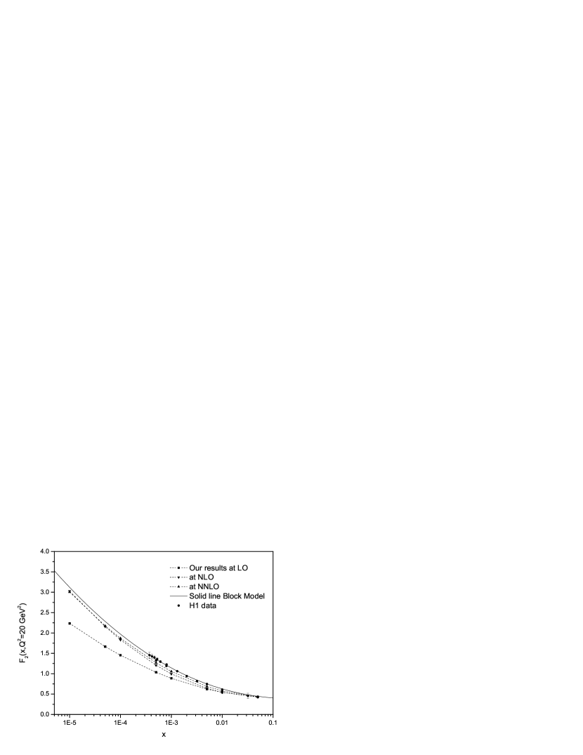
Figure 1: The LO, NLO and NNLO structure functions at $Q^{2}=20\mathrm{GeV}^{2}$. The solid curve is from Block fit [15-16]. The dots are H1 data that accompanied with total errors [26].

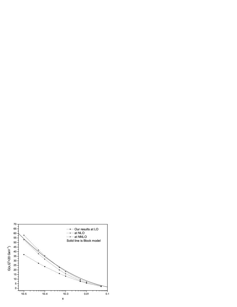
Figure 2: The LO, NLO and NNLO gluon distribution function at $Q^{2}=20\mathrm{GeV}^{2}$. The solid curve is from Block fit [15-16].

In this paper, we found two analytical decoupled solutions for the coupled DGLAP evolution equations for the proton structure function and the gluon distribution function inside the proton. These decoupling equations are directly related to the initial conditions and to the strong interaction coupling constant at LO, NLO and NNLO. To determine the proton structure function and gluon distribution function we need to know only the input singlet and gluon densities and their derivatives at the initial scale of $Q_{0}^{2}$, respectively. The input singlet and gluon parameterizations can be taken from global analysis of the parton distribution functions, in particular from the Block analysis [15,16]. We furthermore follow the DL model [6,7] in taking the hard-Pomeron intercept with $\delta{\simeq}0.5$. We will compare the $x$-space structure function and gluon distribution function calculated from Eqs.15 and 17 at LO up to NNLO starting from the Block initial conditions at $Q_{0}^{2}=1\mathrm{GeV}^{2}$. We will also compare our results with H1 data [26] numerically.
In Figs.1 and 2, we show the results for the proton structure function and gluon distribution function at LO up to NNLO at $Q^{2}=20\mathrm{GeV}^{2}$. The solid curve in these figures is the published Block method [15-16] and also dots are H1 data [26] that accompanied with total errors in Fig.1. In these figures, the squares, down triangles and up triangles are our results for LO, NLO and NNLO from Eqs.15 and 17. We present the results using the $F_{0}(x)$ and $G_{0}(x)$ which are usually taken from the Block model. The agreement between our results at NNLO analysis and the Block method is good. It is clear from these figures for $F_{2}(x,Q^{2})$ and $G(x,Q^{2})$, that our decoupling solutions are correct. As can be seen, the values of the gluon distribution and the proton structure functions increase as $x$ decreases, this is because the hard-Pomeron exchange defined by the DL model is expected to hold in the low-$x$ limit. It is evident from Figs.1 and 2 that three-loop perturbative QCD describes the evolution of the strength of the hard-Pomeron contribution to $F_{2}(x,Q^{2})$ and $G(x,Q^{2})$ very well with respect to the decoupling DGLAP evolution equations.

I.5 Conclusion

We have first developed a method for the analytic solution of the DGLAP evolution equations based on the hard-Pomeron behavior of the parton distributions at low-$x$. In conclusion, we have constructed two decoupled homogeneous second-order differential evolution equations for $F_{2}(x,Q^{2})$ and $G(x,Q^{2})$ from the coupled DGLAP equations at LO up to NNLO analysis, respectively. These results for the gluon distribution and proton structure functions require only a knowledge individual from $G_{0}(x)$, $F_{0}(x)$ and those derivatives at the starting value $Q_{0}^{2}$ for the evolution, respectively. As an illustration of our method, we have used the analytic solutions to the decoupled evolution equations to obtain tests of the consistency our results with published quark and gluon distributions. We demonstrated numerically that the method gives good agreement with published Block method and H1 data at NNLO.

$\bf{Acknowledgements}$ G.R.Boroun would like to thank the anonymous referee of the paper for his/her careful reading of the manuscript and for the productive discussions.

I.6 Appendix A

The explicit forms of the functions $a(x)$, $b(x)$, $c(x)$ and $d(x)$ are

$$\eta(x)=1-a(x)-c(x).$$

$$\zeta(x)=a(x)c(x)-b(x)d(x).$$

$$a(x)=\frac{2}{\beta_{0}}{\int_{x}^{1}}dzP^{LO}_{qq}(z)z^{\delta}.$$

$$b(x)=\frac{2}{\beta_{0}}{\int_{x}^{1}}dzP^{LO}_{qg}(z)z^{\delta}.$$

$$c(x)=\frac{2}{\beta_{0}}{\int_{x}^{1}}dzP^{LO}_{gg}(z)z^{\delta}.$$

$$d(x)=\frac{2}{\beta_{0}}{\int_{x}^{1}}dzP^{LO}_{gq}(z)z^{\delta}.$$ (18)

Where the splitting functions are given by [5,27]

$$P^{\rm LO}_{qq}(z)=C_{F}[\frac{1+z^{2}}{(1-z)_{+}}+\frac{3}{2}\delta(1-z)].$$

$$P^{\rm LO}_{qg}(z)=\frac{1}{2}(z^{2}+(1-z)^{2}).$$

$$P^{\rm LO}_{gq}(z)=C_{F}\frac{1+(1-z)^{2}}{z}.$$

$$P^{\rm LO}_{gg}(z)=2C_{A}(\frac{z}{(1-z)_{+}}+\frac{(1-z)}{z}+z(1-z))$$

$$+\delta(1-z)\frac{(11C_{A}-4N_{f}T_{R})}{6},$$ (19)

with $C_{A}=N_{c}=3$, $C_{F}=\frac{N_{c}^{2}-1}{2N_{c}}=\frac{4}{3}$ and $T_{f}=\frac{1}{2}N_{f}$. The convolution integrals in (18) which contains plus prescription, $()_{+}$, can be easily calculate by [28]

$$\int_{x}^{1}\frac{dy}{y}f(\frac{x}{y})_{+}g(y) = \int_{x}^{1}\frac{dy}{y}f(\frac{x}{y})[g(y)-\frac{x}{y}g(x)]$$

$$-g(x)\int_{0}^{x}f(y)dy$$

I.7 Appendix B

The explicit forms of the functions $M(x,t),N(x,t),P(x,t)$ and $Q(x,t)$ are

$$M(x,t)=-\frac{\alpha_{s}}{2\pi}\int_{x}^{1}{P_{qq}(z,\alpha_{s}(Q^{2}))z^{\delta}dz}.$$

$$N(x,t)=-\frac{\alpha_{s}}{2\pi}\int_{x}^{1}{2N_{f}P_{qg}(z,\alpha_{s}(Q^{2}))z^{\delta}dz}.$$

$$P(x,t)=-\frac{\alpha_{s}}{2\pi}\int_{x}^{1}{P_{gg}(z,\alpha_{s}(Q^{2}))z^{\delta}dz}.$$

$$Q(x,t)=-\frac{\alpha_{s}}{2\pi}\int_{x}^{1}{P_{gq}(z,\alpha_{s}(Q^{2}))z^{\delta}dz}.$$ (21)

where the strong coupling constant,$\alpha_{s}$, up to NNLO is given by Eqs. (6-7). The explicit forms of the second- and third- order splitting functions are respectively [12-14]

$$P_{qq}^{\rm NLO} = (C_{F})^{2}(-1+z+(1/2-3/2z)\ln(z)-1/2(1+z)\ln(z)^{2}-(3/2\ln(z)+2\ln(z)\ln(1-z))p_{qq}(z)$$

$$+2p_{qq}(-z)S_{2}(z))+C_{F}C_{A}(14/3(1-z)+(11/6\ln(z)+1/2\ln(z)^{2}+67/18-\pi^{2}/6)p_{qq}(z)$$

$$-p_{qq}(-z)S_{2}(z))+C_{F}T_{F}(-16/3+40/3z+(10z+16/3z^{2}+2)\ln(z)-112/9z^{2}+40/(9z)$$

$$-2(1+z)\ln(z)^{2}-(10/9+2/3\ln(z))p_{qq}(z)).$$

$$P_{qg}^{\rm NLO} = C_{F}T_{F}(4-9z-(1-4z)\ln(z)-(1-2z)\ln(z)^{2}+4\ln(1-z)+(2\ln((1-z)/z)^{2}-4ln((1-z)/z)$$

$$-2/3\pi^{2}+10)P_{qg}(z))+C_{A}T_{F}(182/9+14/9z+40/(9z)+(136/3z-38/3)\ln(z)-4\ln(1-z)$$

$$-(2+8z)\ln(z)^{2}+2P_{qg}(-z)S_{2}(z)+(-\ln(z)^{2}+44/3\ln(z)-2\ln(1-z)^{2}+4\ln(1-z)$$

$$+\pi^{2}/3-218/9)P_{qg}(z)).$$

$$P_{gq}^{\rm NLO} = C_{F}^{2}(-5/2-7z/2+(2+7/2z)\ln(z)-(1-z/2)ln(z)^{2}-2z\ln(1-z)-(3\ln(1-z)$$

$$+\ln(1-z)^{2})P_{gq}(z))+C_{F}C_{A}(28/9+65/18z+44/9z^{2}-(12+5z+8/3z^{2})\ln(z)+(4+z)\ln(z)^{2}$$

$$+2z\ln(1-z)+S_{2}(z)P_{gq}(-z)+(1/2-2\ln(z)\ln(1-z)+1/2\ln(z)^{2}+11/3\ln(1-z)+\ln(1-z)^{2}$$

$$-\pi^{2}/6)P_{gq}(z))+C_{F}T_{F}(-4/3z-(20/9+4/3\ln(1-z))P_{gq}(z)).$$

$$P_{gg}^{\rm NLO} = C_{F}T_{F}(-16+8z+20/3z^{2}+4/(3z)-(6+10z)\ln(z)-(2+2z)\ln(z)^{2})+C_{A}T_{F}(2-2z$$

$$+26/9(z^{2}-1/z)-4/3(1+z)\ln(z)-20/9P_{gg}(z))+C_{A}^{2}(27/2(1-z)+26/9(z^{2}-1/z)$$

$$-(25/3-11/3z+44/3z^{2})\ln(z)+4(1+z)\ln(z)^{2}+2P_{gg}(-z)S_{2}(z)+(67/9-4\ln(z)\ln(1-z)$$

$$+\ln(z)^{2}-\pi^{2}/3)P_{gg}(z)).$$

where

$$p_{qq}(z)=2/(1-z)-1-z$$

$$p_{qq}(-z)=2/(1+z)-1+z$$

$$P_{qg}(z)=z^{2}+(1-z)^{2}$$

$$P_{qg}(-z)=z^{2}+(1+z)^{2}$$

$$P_{gq}(z)=(1+(1-z)^{2})/z$$

$$P_{gq}(-z)=-(1+(1+z)^{2})/z$$

$$P_{gg}(z)=1/(1-z)+1/z-2+z(1-z)$$

$$P_{gg}(-z)=1/(1+z)-1/z-2-z(1+z)$$

$$S_{2}(z)=\int_{1/(1+z)}^{z/(1+z)}1/y\ln((1-y)/y)dy$$

and

$$P_{qq}^{\rm NNLO} = (N_{f}(-5.926L1^{3}-9.751L1^{2}-72.11L1+177.4+392.9z-101.4z^{2}-57.04L0L1-661.6L0$$

$$+131.4L0^{2}-400/9L0^{3}+160/27L0^{4}-506/z-3584/271/zL0)+N_{f}^{2}(1.778L1^{2}+5.944L1$$

$$+100.1-125.2z+49.26z^{2}-12.59z^{3}-1.889L0L1+61.75L0+17.89L0^{2}+32/27L0^{3}$$

$$+256/811/z))(1-z).$$

$$P_{qg}^{\rm NNLO} = N_{f}(100/27L1^{4}-70/9L1^{3}-120.5L1^{2}+104.42L1+2522-3316z+2126z^{2}$$

$$+L0L1(1823-25.22L0)-252.5zL0^{3}+424.9L0+881.5L0^{2}-44/3L0^{3}+536/27L0^{4}$$

$$-1268.31/z-896/31/zL0)+N_{f}^{2}(20/27L1^{3}+200/27L1^{2}-5.496L1-252+158z+145.4z^{2}$$

$$-139.28z^{3}-L0L1(53.09+80.616L0)-98.07zL0^{2}+11.70zL0^{3}-254L0-98.80L0^{2}-376/27L0^{3}$$

$$-16/9L0^{4}+1112/2431/z).$$

$$P_{gq}^{\rm NNLO} = 400/81L1^{4}+2200/27L1^{3}+606.3L1^{2}+2193L1-4307+489.3z+1452z^{2}+146z^{3}-447.3L0^{2}L1$$

$$-972.9zL0^{2}+4033L0-1794L0^{2}+1568/9L0^{3}-4288/81L0^{4}+6163.11/z+1189.31/zL0$$

$$+N_{f}(-400/81L1^{3}-68.069L1^{2}-296.7L1-183.8+33.35z-277.9z^{2}+108.6zL0^{2}$$

$$-49.68L0L1+174.8L0+20.39L0^{2}+704/81L0^{3}+128/27L0^{4}-46.411/z+71.0821/zL0)$$

$$+N_{f}^{2}(96/27L1^{2}(1/z-1+1/2z)+320/27L1(1/z-1+4/5z)-64/27(1/z-1-2z)).$$

$$P_{gg}^{\rm NNLO} = 2643.524D0+4425.894\delta(1-z)+3589L1-20852+3968z-3363z^{2}+4848z^{3}$$ (24)

$$+L0L1(7305+8757L0)+274.4L0-7471L0^{2}+72L0^{3}-144L0^{4}+142141/z+2675.81/zL0$$

$$+N_{f}(-412.142D0-528.723\delta(1-z)-320L1-350.2+755.7z-713.8z^{2}+559.3z^{3}$$

$$+L0L1(26.15-808.7L0)+1541L0+491.3L0^{2}+832/9L0^{3}+512/27L0^{4}+182.961/z$$

$$+157.271/zL0)+N_{f}^{2}(-16/9D0+6.4630\delta(1-z)-13.878+153.4z-187.7z^{2}+52.75z^{3}$$

$$-L0L1(115.6-85.25z+63.23L0)-3.422L0+9.680L0^{2}-32/27L0^{3}-680/2431/z).$$

where $L0=\ln(z),L1=\ln(1-z)$ and $D0=1/(1-z)$.

I.8 References

1. Yu. L.Dokshitzer, Sov.Phys.JETPG 6, 641(1977 ); G.Altarelli and G.Parisi, Nucl.Phys.B126, 298(1997 ); V.N.Gribov and L.N.Lipatov, Sov.J.Nucl.Phys.28, 822(1978).
2. L.F.Abbott, W.B.Atwood and A.M.Barnett, Phys.Rev.D 22, 582(1980).
3. A.M.Cooper- Sarkar, R.C.E.Devenish and A.DeRoeck, Int.J.Mod.Phys.A 13, 3385( 1998 ); M.Cluck, E.Reya and A.Vogt, Z.Phys.C48,471 (1990); A.D.Martin, W.J.Stirling, and R.S.Thorne, Phys.Lett.B636, 259(2006); A.D.Martin, W.J.Stirling, R.S.Thorne and G.Watt, Eur.Phys.J.C63, 189(2009); A.D.Martin, W.J.Stirling, R.S.Thorne and G.Watt, arXiv:1301.6754(hep-ph); M. Gluck, P. Jimenez-Delgado, E. Reya, Eur.Phys.J.C53, 355(2008); M. Gluck, P. Jimenez-Delgado, E. Reya, Phys.Rev.D79, 074023(2009).
4. K.Prytz, Phys.Lett.B311, 286(1993); K.Prytz. Phys.Lett.B332, 393(1994); M.B. Gay Ducati and V.P.B.Goncalves, Phys.Lett.B390, 401(1997); A.V.Kotikov and G.Parente, Phys.Lett.B379, 195(1996); P.Desgrolard, A.Lengyel and E.Martynov, JHEP 02, 029(2002); A.Donnachie and P.V.Landshoff, Phys.Lett.B 533, 277(2002); J.R.Cudell, A.Donnachie and P.V.Landshoff, Phys.Lett.B 448, 281(1999); J.Kwiecinski, arXiv:hep-ph/9607221(1996).
5. P.D.Collins, An introduction to Regge theory an high-energy physics(Cambridge University Press, Cambridge 1997)Cambridge; M.Bertini et al., Rivista del Nuovo Cimento 19, 1(1996).
6. A.Donnachie and P.V.Landshoff, Z.Phys.C 61, 139(1994); Phys.Lett.B 518, 63(2001).
7.A.Donnachie and P.V.Landshoff, Phys.Lett.B 550, 160(2002); R.D.Ball and P.V.Landshoff, arXiv:hep-ph/9912445.
8. G.Altarelli, G.Parisi, Nucl.Phys.B 126, 298(1977).
9. W.Furmanski, R.Petronzio, Phys.Lett.B 97, 437(1980); R.K.Ellis , W.J.Stirling and B.R.Webber, QCD and Collider Physics(Cambridge University Press,1996).
10. W.L. van Neerven, A.Vogt, Nucl.Phys.B 588, 345(2000).
11. W.L. van Neerven, A.Vogt, Nucl.Phys.B 568, 263(2000).
12. S.Moch, J.Vermaseren and A.Vogt, Nucl.Phys.B 688, 101(2004).
13. S.Moch, J.Vermaseren and A.Vogt, Nucl.Phys.B 691, 129(2004).
14. A.Retey, J.Vermaseren , Nucl.Phys.B 604, 281(2001).
15. M.M.Block, L.Durand and D.W.Mckay, Phys.Rev.D77, 094003(2008).
16. E.L.Berger, M.M.Block, and Chung-I Tan, Phys.Rev.Lett.98, 242001(2007).
17. ZEUS Collaboration, V.Chekanov et.al., Eur.Phys.J.C21, 443(2001).
18. M.Devee, B.Baishya and J.K.sarma, Eur.Phys.J.C72, 2036(2012).
19. S.Weinzierl, arXiv:hep-ph/0203112.
20.M.M.Block, L.Durand, P.Ha and D.W.Mckay, arXiv:hep-ph/1004.1440(2010); arXiv:hep-ph/1005.2556(2010)
21. G.R.Boroun, JETP106, 700(2008); B.Rezaei and G.R.Boroun, JETP112, 381(2011); G.R.Boroun and B.Rezaei, Eur.Phys.J.C.72, 2221(2012).
22. W.L. van Neerven, E.B. Zijlstra, Phys.Lett.B272, 127 (1991); E.B. Zijlstra, W.L. van Neerven, Phys.Lett.B273, 476(1991); Phys. Lett. B297, 377(1992); Phys.Lett.B383, 525(1992).
23. R. Hamberg, W.L. van Neerven, T. Matsuura, Nucl.Phys.B359, 343(1991); R. Hamberg, W.L. van Neerven, T. Matsuura, Nucl.Phys.B644, 403(2002), Erratum; R.V. Harlander, W.B. Kilgore, Phys.Rev.Lett.88, 201801(2002), hep-ph/0201206.
24. B.G. Shaikhatdenov, A.V. Kotikov, V.G. Krivokhizhin, and G. Parente, Phys.Rev.D81, 034008(2010).
25. A.Donnachie and P.V.Landshoff, Phys.Lett.B296, 257(1992); P.Desgrolard, M. Giffon, E.Martynov and E .Predazzi, Eur.Phys.J.C18, 555(2001); P.Desgrolard, M. Giffon and E.Martynov, Eur.Phys.J.C7, 655(1999); A.D.Martin, M.G.Ryskin and G.Watt, arXiv:hep-ph/0406225.
26.F.D. Aaron et al. [H1 Collaboration], Eur.Phys.J.C71,1579(2011); C.Adloff et al. [H1 Collaboration], Eur.Phys.J.C21, 33(2001).
27.R.G.Roberts, The structure of the proton(Cambridge University Press,1990).
28.B.Lampe, E.Reya, Phys.Rep.332, 1(2000).