Laguerre polynomials method in valon model

Abstract

We used the Laguerre polynomials method for determination of the proton structure function in the valon model. We have examined the applicability of the valon model with respect to a very elegant method, where the structure of the proton is determined by expanding valon distributions and valon structure functions on Laguerre polynomials. We compared our results with the experimental data, GJR parameterization and DL model. Having checked, this method gives a good description for the proton structure function in valon model.

Department of Physics, Razi University, Kermanshah 67149, Iran

Keywords: Valon model, Structure function, Laguerre polynomials.

1. Introduction

Structure functions in lepton-nucleon deep-inelastic scattering (DIS) are the established observables probing Quantum Chromodynamics (QCD), the theory of the strong interaction, and in particular the structure of the nucleon. The structure functions provide unique information about the deep structure of the hadrons and most importantly, they form the backbone of our knowledge of the parton densities. In QCD, structure functions are defined as convolution of the universal parton momentum distributions inside the proton and coefficient functions, which contain information about the boson-parton interaction. The parton distributions in proton have been studied extensively in a wide range of both $x$ and $Q^{2}$, as they are accurate but inconvenient to describe analytically. Here we elaborate on the valon model that can be very useful in the study of hadronic structure, in particular when the experimental data are scarce. A valon has its own cloud of partons which can be calculated in pQCD. This structure is universal and independent of the hosting hadron [1-2].
The valon model [1-4] is a phenomenological model which is proven to be very useful in its application to many areas of the hadron physics. A valon is defined to be a dressed valence quark in QCD with a cloud of gluons and sea quarks and antiquarks. Its structure can be resolved at high enough $Q^{2}$ probes. In the scattering process the virtual emission and absorption of gluon in a valon becomes bremsstrahlung and pair creation, which can be calculated in QCD. At sufficiently low $Q^{2}$ the internal structure of a valon cannot be resolved and hence, it behaves as a structureless valence quark. At such a low value of $Q^{2}$, the nucleon is considered as bound state of three valons, UUD for proton. The binding agent is assumed to be very soft gluons or pions. Let us denote the distribution of a valon in a nucleon by $G_{\frac{v}{N}}(y)$ for each valon $v$. It satisfies the normalization condition, $\int_{0}^{1}G_{\frac{v}{N}}(y)dy=1$ and the momentum sum rule $\sum_{v}\int_{0}^{1}G_{\frac{v}{N}}(y)dy=1$, where the sum runs over all valons in nucleon $N$. The organization of the paper is as follows; in section 2 we will give a brief description of the valon model. In section 3 we consider the Laguerre polynomials method which this work is based on, then we will calculate the nucleon structure in terms of the valon distributions and the valon structure functions on Laguerre polynomials. Finally, in section 4, the numerical calculations will be outlined; then we discuss some qualitative implications of the Laguerre polynomials method on the structure of the nucleon in valon model.

2. Valon distribution and Valon structure function

In the preceding section, we discussed the valon structure of a nucleon. In this subsection we will give the distributions in a valon. The nucleon structure function is related to the valon structure function by the convolution theorem as follows [1-5],

$$\ F_{2}^{N}(x,Q^{2})=\sum_{v}\int^{1}_{x}G_{\frac{v}{N}}(y)F_{2}^{v}(\frac{x}{y},Q^{2})\frac{dy}{y}$$ (1)

where the summation is over the three valons, and $G_{\frac{v}{N}(y)}$ is the probability of finding a valon that carrying momentum fraction y of the hadron, and also $F_{2}^{v}(\frac{x}{y},Q^{2})$ is the structure function of a valon. The structure function of a U-type valon can be written as:

$$\ F^{U}_{2}(z,Q^{2})=\frac{4}{9}z(G_{\frac{u}{U}}+G_{\frac{\bar{u}}{U}})+\frac{1}{9}z(G_{\frac{d}{U}}+G_{\frac{\bar{d}}{U}}+G_{\frac{s}{U}}+G_{\frac{\bar{s}}{U}}),$$ (2)

where G’s are valence and sea quark distribution functions, and defined the probability function for $v$-valon to have a momentum fraction $z$ in the nucleon. A similar expression can be written for the D-type valon. Structure of a valon can be written in terms of favored distribution ($G_{f}$) and unfavored distribution ($G_{nf}$), as for D and U valon structure functions we have [1-5]

$$\ F^{U}_{2}(z,Q^{2})=\frac{4}{9}z[G_{f}(z,Q^{2})+2G_{nf}(z,Q^{2})].$$ (3)

$$\ F^{D}_{2}(z,Q^{2})=\frac{1}{9}z[G_{f}(z,Q^{2})+11G_{nf}(z,Q^{2})],$$ (4)

or

$$\ F^{U}_{2}(z,Q^{2})=\frac{2}{9}z[G^{S}(z,Q^{2})+G^{NS}(z,Q^{2})],$$ (5)

$$\ F^{D}_{2}(z,Q^{2})=\frac{1}{9}z[2G^{S}(z,Q^{2})-G^{NS}(z,Q^{2})],$$ (6)

where $G^{S}$and $G^{NS}$ are defined by singlet and nonsinglet components respectively. The relation between favored and unfavored distributions with singlet and nonsinglet distributions have the following forms:

$$\ G_{f}=\frac{1}{2f}[G^{S}+(2f-1)G^{NS}],$$ (7)

$$\ G_{uf}=\frac{1}{2f}[G^{S}-G^{NS}],$$ (8)

where f is number of active flavors (f=3 or f=4). In the momentum representation we have

$$\ M_{2}(n,Q^{2})=\int^{1}_{0}x^{n-2}F_{2}(x,Q^{2})dx,$$ (9)

and

$$\ M_{\alpha}(n,Q^{2})=\int^{1}_{0}x^{n-1}G_{\alpha}(x,Q^{2})dx$$ (10)

where $\alpha=\frac{v}{N},S,NS$. In order to estimate of the structure function momentums, inserting Eqs.(9) and (10) in Eq. (1), as we obtain:

$$\ M^{p}(n,Q^{2})=\sum_{v}M_{\frac{v}{p}}(n)M^{v}(n,Q^{2}).$$ (11)

We assume a general parameterization form for U and V valons as follows:

$$\ G_{\frac{UUD}{p}}(y_{1},y_{2},y_{3})=\alpha(y_{1}y_{2})^{a}y_{3}^{b}\delta(y_{1}+y_{2}+y_{3}-1),$$ (12)

where a and b are the two free parameters that can be evaluated from the experimental data, and also $\alpha$ is a normalization coefficient. Here $y_{i}$ is the momentum fraction of the i^,th valon. The $U$- and $D$-type valon distributions can be obtained by integration over the specified variable as:

$$\ G_{\frac{U}{p}}(y)=\int dy_{2}dy_{3}G_{\frac{UUD}{p}}(y,y_{2},y_{3})=B(a+1,a+2,2)^{-1}y^{a}(1-y)^{a+b+1},$$ (13)

$$\ G_{\frac{D}{p}}(y)=\int dy_{1}dy_{2}G_{\frac{UUD}{p}}(y_{1},y_{2},y)=B(b+1,2a+2)^{-1}y^{b}(1-y)^{2a+1},$$ (14)

where $B(m,n)$ is the Euler beta- function. The normalization factor has been fixed by requiring

$$\int_{0}^{1}G_{\frac{U}{P}}(y)dy=\int_{0}^{1}G_{\frac{D}{P}}(y)dy=1.$$ (15)

Consequently, the moments of theses valon distributions are calculated [1-6] according to the Mellin transformation from Eq.(10) for nucleon

$$\ U(n)=\frac{B(a+n,a+b+2)}{B(a+1,a+b+2)},$$ (16)

$$\ D(n)=\frac{B(b+n,2a+2)}{B(b+1,2a+2)},$$ (17)

with $a=0.65$ and $b=0.35$. Therefore, the valon distributions can be obtained as,

$$\ G_{\frac{U}{p}}=7.98y^{0.65}(1-y)^{2},$$ (18)

$$\ G_{\frac{D}{p}}=6.01y^{0.35}(1-y)^{2.3}.$$ (19)

Now, we can go to the N-moment space for define the moments of these quark distribution functions (valence, sea , and gluons)[5,7-8] as:

$$\ M_{u_{v}}(n,s)=2U(n)M^{NS}(n,s),$$ (20)

$$\ M_{d_{v}}(n,s)=D(n)M^{NS}(n,s),$$ (21)

$$\ M_{sea}(n,s)=(2f)^{-1}[2U(n)+D(n)][M^{S}(n,s)-M^{NS}(n,s)],$$ (22)

$$\ M_{g}(n,s)=[2U(n)+D(n)]M_{gq}(n,s),$$ (23)

where $M^{S}$ and $M^{NS}$ are the moments of the singlet and nonsinglet valon structure functions and $M_{gq}(n,s)$ is the quark-to-gluon evolution function and defined into $d_{NS}$, $d_{+(-)}$, $d_{gq}$ and $\rho$ where they are anamolus dimensions [1-2,5,7-8] as follows:

$$\ M^{NS}(n,s)=e^{-d_{NS}s},$$ (24)

$$\ M^{S}(n,s)=\frac{1}{2}(1+\rho)e^{-d_{+}s}+\frac{1}{2}(1-\rho)e^{-d_{-}s},\leavevmode\nobreak\ \leavevmode\nobreak\ \leavevmode\nobreak\ \leavevmode\nobreak\ \leavevmode\nobreak\ \leavevmode\nobreak\ M_{gq}(n,s)=(d_{+}-d_{-})^{-1}d_{gq}[e^{-d_{+}s}-e^{-d_{-}s}].$$ (25)

Here, $s$ is defined by:

$$\ s=\ln[\frac{\ln(\frac{Q^{2}}{\Lambda^{2}})}{\ln(\frac{Q_{0}^{2}}{\Lambda^{2}})}],$$ (26)

where $Q^{2}_{0}$ and $\Lambda$ are our initial scales. In determining of the parton distributions, we have used a fit to a set of the experimental data [9-10] for a single value of $s$ or $Q^{2}$. Then we fit the moments by a beta function that are the moments of the forms [3-4,6]:

$$\ xq_{v}(x)=a(1-x)^{b}x^{c},$$ (27)

$$\ x{q}_{i}(x)=a_{i}x^{b_{i}}(1-x)^{c_{i}}(1+d_{i}x+e_{i}x^{0.5}),$$ (28)

where, the subscript $i$ stand for $sea$ or $gluon$, and $xq_{i}$^,s are the sea and gluon distribution functions. The free parameters in Eqs.(27) and (28) are further considered to be functions of $s$, as they are given in the Appendix. Therefore we obtained the parton distributions for any valon that can be used in the valon structure function.

3. Laguerre Polynomials to valon model

So far, the structure of a nucleon into the valon distributions is determined. Now we will use an elegant and fast numerical method for determination of the proton structure function in valon model. Therefore, we concentrate on the Laguerre polynomials in our determinations. In the laguerre polynomials method [11-12], the Laguerre polynomials are defined as:

$$\ (n+1)L_{n+1}(x)=(2n+1-x)L_{n}(x)-nL_{n-1}(x),$$ (29)

and orthogonality condition is defined as:

$$\ \int^{\infty}_{0}e^{-{\acute{x}}}L_{n}(\acute{x})L_{m}(\acute{x})d\acute{x}=\delta_{n,m}.$$ (30)

The general integrable function $f(e^{-\acute{x}})$ is transformed into the sum:

$$\ f(e^{-\acute{x}})=\sum^{N}_{0}f(n)L_{n}(\acute{x}),$$ (31)

where

$$\ f(n)=\int^{\infty}_{0}e^{-\acute{x}}L_{n}(\acute{x})f(e^{-\acute{x}})d\acute{x}.$$ (32)

In what follows we want to calculate the proton structure function in valon model using the Laguerre polynomials method. We used the variable transformations, $x=e^{-\acute{x}}$ , $y=e^{-\acute{y}}$ to get the valonic structure function form to the Laguerre polynomials form. Then, we combined and expand each term of this equation on Laguerre polynomials according to Eqs.(31)-(32) and using this properties as:

$$\int^{\acute{x}}_{0}d\acute{y}L_{n}(\acute{x}-\acute{y})L_{m}(\acute{y})=L_{n+m}(\acute{x})-L_{n+m+1}(\acute{x}).$$ (33)

We obtained an equation which determines $F^{p}_{2}(x,Q^{2})$ in terms of the Laguerre polynomials, namely:

$$F^{p}_{2}(n,Q^{2})=\sum_{v}\sum^{n}_{m=0}\tilde{G}_{\frac{v}{p}}(m)[F^{v}_{2}(n-m,Q^{2})-F^{v}_{2}(n-m-1,Q^{2})],$$ (34)

where

$$\ F^{v}_{2}(n,Q^{2})=\int^{\infty}_{0}d\acute{x}e^{-\acute{x}}F^{v}_{2}(e^{-\acute{x}},Q^{2})L_{n}(\acute{x}),$$ (35)

and

$$\tilde{G}_{\frac{v}{p}}(m)=\int^{\infty}_{0}d\acute{y}e^{-\acute{y}}{G}_{\frac{v}{p}}(e^{-\acute{y}})L_{m}(\acute{y}),$$ (36)

as $F^{v}_{2}(x)$ is defined according to Eqs.(3) and (4) which are accompanied with respect to Eqs.(27) and (28) and their coefficients according to appendix, and also ${G}_{\frac{v}{p}}(y)$ is defined according to Eqs.(18) and (19) respectively. Therefore we find the solution of the proton structure function in valon model defined by solving this recursion relation as:

$$\ F^{p}_{2}(x,Q^{2})=\sum_{n=0}^{N}F^{p}_{2}(n,Q^{2})L_{n}(Ln\frac{1}{x}),$$ (37)

where $F^{p}_{2}(n,Q^{2})$ is the proton structure function with respect to the Laguerre model and its defined by Eqs.(34)-(36) as the coefficients in these equations are obtained with respect to the valon model. This result is completely general and gives the expression for the proton structure function with respect to the Laguerre polynomials model. Here we can expand the integrable functions till a finite order $N=30$, as we can convergence these series in the numerical determinations.

4. Results and Discussion

We computed the predictions for all detail of the proton structure function in the kinematic range where it has been measured by $H1$ Collaboration [9-10] and compared with DL model [13-15] based on hard Pomeron exchange, and with GJR parametrization[16]. Our numerical predictions are presented as functions of $x$ for the $Q^{2}=$22.5 $GeV^{2}$. The results are presented in Fig.1 where they are compared with the $H1$ data and with the results obtained with the help of other standard parameterizations. The curves represent the proton structure functions based on a fit to all data. We compared our results with predictions of $F_{2}^{p}$ in perturbative QCD where the input densities are given by GJR parameterizations [16]. Also, we compared our results with the two pomeron fits as seen in Fig.1. The agreement between the Laguerre polynomials method for the proton structure function in valon model and data at low and high -$x$ is remarkably good, as at low $x$ the gluon distributions are dominate. Therefore, the good agreement indicates that the Laguerre polynomials method in valon model for the proton structure function has a good asymptotic behavior and it is compatible with both the data and the other standard models at $x$ values. As this model has this advantage that we get a very elegant solution for the proton structure function. Fig.2 shows the shape of the distribution functions in Eqs.(27) and (28) for the valence and the sea quarks at $Q^{2}=22.5GeV^{2}$.
In summary, we have used the Laguerre polynomials method to describe the proton structure function in valon model. The proton structure can be determined in terms of the valon distributions and the valon structure functions with respect to Laguerre polynomials. To confirm the method and results, the calculated values are compared with the H1 data on the proton structure function. It is shown that, there is a good agreement with experimental H1 data for $F_{2}^{p}$, if one takes into the total errors, and is consistent with a higher order QCD calculations of $F_{2}^{p}$ which essentially show increase as $x$ decreases. We observed that the calculations results are consistent with the two pomeron model. Thus implying that Regge theory and perturbative evolution may be made compatible at small-x. Also this model gives a good description of the parton distributions at low and high- $x$ values.

Appendix

Here we will give the functional form of parameters of Eqs.(27)-(28) by the following forms in terms of $s$. Coefficients for u valance in U valon are:

$$a_{u}=16.860-8.382s+1.352s^{2},$$

$$b_{u}=1.775+0.693s+0.014s^{2},$$

and

$$c_{u}=1.794-0.699s+0.104s^{2}.$$

Coefficients for d valance in D valon are:

$$a_{d}=13.119-8.66s+1.65s^{2},$$

$$b_{d}=7.129-3.5s+0.901s^{2},$$

and

$$c_{d}=1.971-0.9502s+0.163s^{2}.$$

Coefficients for sea quarks in each valon are:

$$a_{sea}=-0.206+0.190s-0.022s^{2},$$

$$b_{sea}=-0.884+0.484s-0.104s^{2},$$

$$c_{sea}=12.089-4.532s+0.939s^{2},$$

$$d_{sea}=-2.564+5.937s-1.531s^{2},$$

and

$$e_{sea}=-8.623+4.9823s-1.123s^{2}.$$

Coefficients for gluons in each valon are:

$$a_{gluon}=13.8745-22.3304s+12.7885s^{2}-2.4801s^{3},$$

$$b_{gluon}=4.6810-8.4594s+4.7656s^{2}-0.9209s^{3},$$

$$c_{gluon}=-24.5652+50.4661s-30.147s^{2}+6.0738s^{3},$$

$$d_{gluon}=-0.8839+0.0403s-0.0174s^{2}.$$

$\bf{Acknowledgements}$ G.R.Boroun would like to thank Dr.M.Tabrizi for computer proceeding and Dr.H.Khanpour for fruitful discussions on QCD fits, and also Dr.B.Rezaei for reading and correcting the manuscript of this paper and for productive discussions.

Figure 1: Comparing of the proton structure function by using the Laguerre polynomials in valon model, with the experimental data [9-10] and DL model [13-15] and GJR parameterization [16] at $Q^{2}=22.5GeV^{2}$.

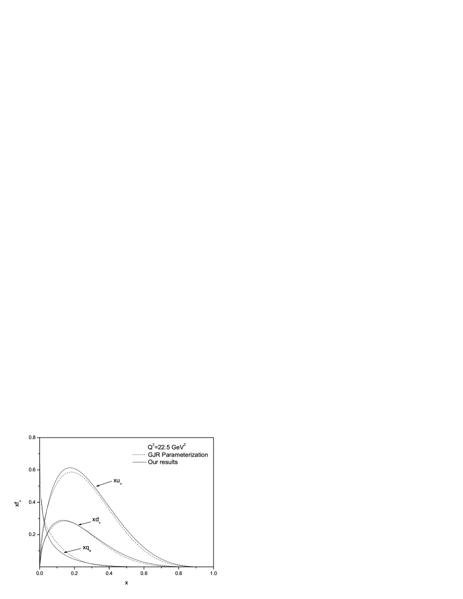
Figure 2: Comparing of the parton distributions in proton with GJR parameterization [16] at $Q^{2}=22.5GeV^{2}$.

References

- [1] R.C.Hwa, phys.Rev.D22, 1593(1980); phys.Rev.D51, 85(1995).
- [2] Rudolph Hwa and C.B.Yang, phys. Rev. C66, 025204(2002); phys. Rev. C66, 025205(2002).
- [3] Firooz Arash, arXiv:hep-ph/0307247V1,19Jul, 2003;Firooz Arash and Ali.N.khorramian, phys. Rev. C67, 045201(2003); Firooz Arash and Ali.N.khorramian, arXiv:hep-ph/990424V1,7Apr,1999; arXiv:hep-ph/9909328V1,11Sep, 1999.
- [4] Firooz Arash, Phys. Lett. B557, 38(2003); Phys.Rev. D9, 054024(2004).
- [5] R.C.Hwa and S.Zahir, Phy. Rev D,V23, 2539(1981); R.C.Hwa and C.S.Lam, Phy. Rev D,V26, 2338(1982).
- [6] A.Mirjalili, et.al., J.Phys.G:Nucl.Part.Phys37, 105003(2010).
- [7] T.A.Degrand,Nucl.Phys. B 151,485(1979).
- [8] I.Hinchliffe and C.H.Llewellyn Smith,B 128, 93(1977).
- [9] E665 Collab (Adams et al) Phys. Rev. Lett 75,1466(1995); H1 collab (Ahmed et al) Nucl. Phys. B439, 471(1995).
- [10] C.Adloff, H1 Collab., Eur.Phys.J.C21, 33(2001).
- [11] Laurent Schoeffel, Nucl.Instrum.Meth.A423, 439( 1999); C.Coriano and C.Savkli, Comput.Phys.Commun.118, 236(1999).
- [12] B.Rezaei and G.R.Boroun, Nucl.Phys.A 857, 42(2011).
- [13] A.Donnachie and P.V.Landshoff, Phys. Lett.B 296, 257(1992).
- [14] A.Donnachie and P.V.Landshoff, Phys. Lett.B 437, 408(1998).
- [15] A.Donnachie and P.V.Landshoff, Phys. Lett.B 550, 160 (2002);P.V.Landshoff ,arXiv:hep-ph/0203084.
- [16] M. Gluck, P. Jimenez-Delgado, E. Reya, Eur.Phys.J.C 53,355 (2008).