The Norma cluster (ACO 3627) – III. The Distance and Peculiar Velocity via the Near-Infrared $\mn@boldsymbol{K_{s}}$-band Fundamental Plane.

Abstract

While Norma (ACO 3627) is the richest cluster in the Great Attractor (GA) region, its role in the local dynamics is poorly understood. The Norma cluster has a mean redshift (z_CMB) of 0.0165 and has been proposed as the “core” of the GA. We have used the $K_{s}$-band Fundamental Plane (FP) to measure Norma cluster’s distance with respect to the Coma cluster. We report FP photometry parameters (effective radii and surface brightnesses), derived from ESO NTT SOFI images, and velocity dispersions, from AAT 2dF spectroscopy, for 31 early-type galaxies in the cluster. For the Coma cluster we use 2MASS images and SDSS velocity dispersion measurements for 121 early-type galaxies to generate the calibrating FP dataset. For the combined Norma-Coma sample we measure FP coefficients of $a$ $=$ $1.465$ $\pm$ $0.059$ and $b$ $=$ $0.326$ $\pm$ $0.020$. We find an rms scatter, in $\log\sigma$, of $\sim$ 0.08 dex which corresponds to a distance uncertainty of $\sim$ 28% per galaxy. The zero point offset between Norma’s and Coma’s FPs is $0.154$ $\pm$ $0.014$ dex. Assuming that the Coma cluster is at rest with respect to the cosmic microwave background frame and z_CMB(Coma) = 0.0240, we derive a distance to the Norma cluster of $5026$ $\pm$ $160$ km s^-1, and the derived peculiar velocity is $-72$ $\pm$ $170$ km s^-1, i.e., consistent with zero. This is lower than previously reported positive peculiar velocities for clusters/groups/galaxies in the GA region and hence the Norma cluster may indeed represent the GA’s “core”.

1 Introduction

By studying the sky distribution of the Sc galaxy sample of Rubin et al. (1976) and the southern group catalogue of Sandage (1975), Chincarini & Rood (1979) found evidence for a supercluster in the Hydra-Centaurus region. This supercluster encompasses the rich clusters now catalogued as Abell S0636 (Antlia, $v_{\rm{hel}}$ $\simeq$ 2800 km s^-1), Abell 1060 (Hydra, $v_{\rm{hel}}$ $\simeq$ 3800 km s^-1), Abell 3526 (Centaurus, $v_{\rm{hel}}$ $\simeq$ 3400 km s^-1) and Abell 3574 (IC4329, $v_{\rm{hel}}$ $\simeq$ 4800 km s^-1). The Local Supercluster has a sizable motion ($\sim$ 300 km s^-1) towards this supercluster (Shaya, 1984; Tammann & Sandage, 1985) and the galaxy motions in the Local Supercluster have a shear that is directed towards Hydra-Centaurus (Lilje, Yahil & Jones, 1986). From a redshift survey of the Hydra-Centaurus region, da Costa et al. (1986) concluded that this supercluster extends to $v_{\rm{hel}}$ $\simeq$ 5500 km s^-1.

The discovery of large positive streaming motions in the Hydra-Centaurus direction (Lynden-Bell et al., 1988) led to the idea of a large, extended mass overdensity, i.e., the Great Attractor (GA), dominating the local dynamics. They found a surprisingly large positive peculiar velocity for the dominant Cen30 sub-component of the Centaurus cluster, i.e., +1100 $\pm$ 208 km s^-1. While several studies confirmed the presence of these large positive peculiar velocities, e.g., Aaronson et al. (1989); Dressler & Faber (1990), a non-significant peculiar velocity for Cen30 of +200 $\pm$ 300 km s^-1 was measured by Lucey & Carter (1988) (c.f. Burstein, Faber & Dressler 1990).

Subsequently the SPS redshift survey (supergalactic plane redshift survey, Dressler, 1988) and the redshifts of IRAS galaxies in this region (Strauss & Davis, 1988) confirmed that there was a substantial concentration of galaxies in this region extending from 2000 to 5500 km s^-1. While in the literature the GA term has been used differently by various studies (see Lynden-Bell et al. 1989; Burstein et al. 1990; Rowan-Robinson et al. 1990; Mould et al. 2000; Courtois et al. 2012, 2013), an inclusive definition for the GA is the mass contained in the volume spanning $\ell$ = 260 to 350^∘, $b$ = –35 to 45^∘, $v_{\rm{hel}}$ = 2000 to 6000 km s^-1. This broad definition encompasses the Hydra-Centaurus supercluster but extends across the galactic plane to include Pavo-I, Pavo-II and the Norma cluster.

After more than two decades of study the nature and full extent of the GA is still not well established. The original work by Lynden-Bell et al. (1988) estimated the GA to have a mass of $\sim$ $5.4\times 10^{16}\rm M_{\odot}$, centred at ($\ell$, $b$) $=$ (307^∘, 9^∘) and $v_{\rm{hel}}$ $=$ $4350$ $\pm$ $350$ km s^-1. From SBF (surface brightness fluctuation) distances for $\sim$ 300 early-type galaxies (ETGs) Tonry et al. (2000) place the GA at ($\ell$, $b$, $v_{\rm{hel}}$) $=$ ($289^{\circ}$, $19^{\circ}$, $3200\pm 260$ km s^-1) with a mass $\sim 8\times 10^{15}\rm M_{\odot}$, i.e., approximately six times less than the original derived mass. As the GA spans low galactic latitudes, where the extinction is severe, our understanding of this important local large structure is still incomplete.

Beyond the GA at ($l$, $b$, $v_{\rm{hel}}$) = (312^∘, 31^∘, 14400 km s^-1) lies the extremely rich Shapley Supercluster. While first recognised by Shapley (1930) as a very populous cloud of galaxies, this structure was highlighted by Oort (1983) in his review of superclusters. With the publication of the southern extension to the Abell cluster catalogue (Abell, Corwin Jr. & Olowin, 1989) a large number of rich clusters in Shapley was noted (Scaramella et al., 1989). Raychaudhury (1989) from an analysis of galaxies on the UKST survey plates independently found this remarkable structure.

The role of Shapley in the local dynamics is unclear. While most studies concluded/advocated that Shapley has only a modest contribution ($\leq$100 km s^-1) to Local Group motion with respect to the CMB, e.g., Ettori et al. (1997); Branchini et al. (1999); Hudson et al. (2004), some studies have concluded a much larger contribution ($\sim$ 300  km s^-1), see, e.g., Marinoni et al. (1998); Kocevski & Ebeling (2006). The lack of clear evidence for any backside infall into the GA (Mathewson et al., 1992; Hudson, 1994) led to the idea that the Shapley supercluster dominates the motions on the farside of the GA (Allen et al., 1990). Extensive redshift surveys (e.g., Radburn-Smith et al. 2006; Proust et al. 2006) have revealed the complex interconnections of the structures in this region.

The Norma cluster (Abell 3627) was identified by Kraan-Korteweg et al. (1996) as the richest cluster in the GA region lying close to the galactic plane at ($\ell$, $b$, $v_{\rm{hel}}$) $=$ (325^∘, -7^∘,  4871 km s^-1) (Woudt et al., 2008). Norma’s mass and richness is comparable to the Coma cluster (Woudt et al., 2008). How the observed motions in the GA region relate to Norma is of great interest and this can be investigated via the measurement of Norma’s peculiar velocity. In general, if Norma is indeed located near the core of the “classical” GA overdensity, then this cluster is likely to possess a small peculiar velocity. Whereas if, for example, the relatively nearby GA model of Tonry et al. (2000) is correct, then the Norma cluster might be expected to have a negative peculiar velocity of the order of –500 km s^-1. Alternatively, if a sizable component of the observed GA flow were due to a large-scale bulk flow caused by the distant Shapley supercluster then the Norma cluster would possess a sizable positive motion of the order of +500 km s^-1. The large-scale peculiar velocity field derived from density field reconstructions predict that Norma’s peculiar velocity is less than 100 km s^-1 (Branchini et al. 1999, PSCz and Lavaux et al. 2010, 2MRS).

There has been keen interest in the Norma cluster, with dedicated multi-wavelength studies, for example X-ray (Boehringer et al., 1996), Hi (Vollmer et al., 2001), deep optical surveys (Woudt & Kraan-Korteweg, 2001), a deep redshift survey (Woudt et al., 2008, hereafter Paper I) and near-infrared (Skelton, Woudt & Kraan-Korteweg, 2009).

In this third paper we report Norma’s distance (and hence peculiar velocity) derived from distance measurements of early-type cluster galaxies. We use both the Fundamental Plane (Djorgovski & Davis, 1987; Dressler et al., 1987) and the metric aperture Faber-Jackson relation (Faber & Jackson, 1976; Lucey, 1986). We apply these techniques using NIR $K_{s}$-band photometry where the effect of foreground galactic extinction is only $\sim$ 0.07 mag. We determine Norma’s distance relative to the Coma cluster which we assume is at rest with respect to the CMB frame; various measurements support this assumption, e.g., (Colless et al., 2001; Bernardi et al., 2002; Hudson et al., 2004; Springob et al., 2007).

This paper is structured as follows. Sample selection, observations, and spectroscopic data analysis are discussed in $\S$ ​2. The photometric analysis is discussed in $\S$ ​3. In $\S$ ​4, we discuss the methods used to determine the zero-point offset, and thereafter turn the zero-point offset into a distance and peculiar velocity ($\S$​ 5). We finally discuss our results under $\S$ ​6.

We have adopted, where not stated, standard cosmology with $H_{0}=70.5\;\rm{km}\;\rm s^{-1}\!\;\rm{Mpc}^{-1}$, $\Omega_{\text{m}}=0.27$, and $\Omega_{\Lambda}=0.73$ (Hinshaw et al., 2009). For the Coma cluster we adopt a redshift (z${}_{{}_{\rm{CMB}}}$) of 0.0240 which results in an angular diameter distance of 99.2 Mpc and a scale of $1^{\prime\prime}$ = 0.481 kpc for Coma.

2 Sample Selection, Observations and Data Reduction

2.1 Sample selection (photometry)

The Norma cluster has a mean heliocentric velocity ($v_{\rm hel}$) of 4871 $\pm$ 54 km s^-1 and a velocity dispersion ($\sigma_{\rm cl}$) of 925 km s^-1 (Paper I). For our Norma ETG sample we selected galaxies that

1. had velocities within $\pm$ 3 $\sigma_{\rm cl}$ of $v_{\rm hel}$, i.e., the velocity range 2096 km s^-1 $<v_{\rm hel}<$ 7646 km s^-1,

2. were within the Abell radius ($R_{A}$ = 1$.\!\!^{\circ}$74), and

3. we had successfully measured a central velocity dispersion for (see $\S$2.2).

This resulted in a sample of 31 ETGs. Figure 1 (left panel) shows the sky distribution of our sample; all galaxies lie within 0.6 $R_{A}$. Figure 1 (right panel) shows the velocity distribution of the sample which is very similar to the distribution of the 296 known cluster members.

For our Coma cluster ETG sample we selected galaxies that

1. were typed as E or E/S0 or S0 by Dressler (1980),

2. were redshift-confirmed cluster members,

3. had a central velocity dispersion in SDSS DR8 (Aihara et al., 2011) and

4. we were successfully able to measure the FP photometry parameters from the 2MASS Atlas images (see $\S$ 2.3).

This resulted in a sample of 121 ETGs.

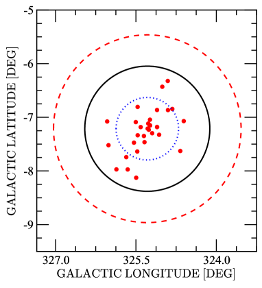
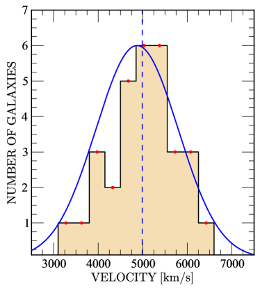
Figure 1: The sample selection for the Norma cluster NIR $K_{s}$-band FP. In the left panel, the outer dashed circle corresponds to the Abell radius, $R_{A}$, the black solid and the blue dotted circles correspond to $\frac{2}{3}R_{A}$ and $\frac{1}{3}R_{A}$, respectively. The red filled circles show the positions of the 31 ETGs. The right panel shows the corresponding velocity distribution; the over-plotted Gaussian (blue solid curve) corresponds to the mean heliocentric velocity and central velocity dispersion for the Norma cluster as measured from 296 cluster member galaxies (Paper I). The blue vertical dotted line represents the mean heliocentric velocity of our Norma cluster FP sample.

2.2 Spectroscopic data

Fibre spectroscopy was undertaken with the 2dF facility (Lewis et al., 2002) on the 3.9 m Anglo-Australian Telescope. For the Norma cluster three fibre configurations were used. This enabled repeat observations of Norma’s ETGs for velocity dispersion measurements as well as an in-parallel redshift survey of the cluster (see Paper I). Immediately before the observations of the Norma cluster, two fibre configurations centred on the Centaurus cluster (Abell 3526) were observed to calibrate the measured velocity dispersions onto a standardised system. Along with these science frames, observations were also made of four K-giant stars (to act as templates for the cross-correlation) as well as offset sky and flat-field frames.

The 2 $\aas@@fstack{\prime\prime}$1 diameter of the 2dF fibres translates into a physical size of 0.70 kpc at the Norma redshift. As described in Paper I, the observations were made with the 1200V gratings which resulted in a wavelength coverage of 4700–5840Å at a FWHM resolution of 125 km s^-1 at Mg $b$; this is sufficient to determine velocity dispersions down to $\sim$ 60 km s^-1. Spectra were extracted from the raw data frames, flat-fielded, wavelength calibrated and sky-subtracted using the AAO 2dfdr software package. After redshift determination via cross-correlation, the spectra were shifted to a rest-frame wavelength and continuum subtracted. Velocity dispersions ($\sigma$) were measured by comparing galaxy spectra to those of the stellar templates, using the Fourier quotient method of Sargent et al. (1977). Errors were determined by bootstrap re-sampling the spectra.

Systematic offsets in velocity dispersion measurements at the level of $\sim$ 0.015 dex exist between different observing systems (telescopes, spectrographs, runs, etc). The SMAC project (Hudson et al., 2001) intercompared measurements from 27 different systems and constructed a standardized system of velocity dispersions. Our Centaurus velocity dispersion measurements were used to calibrate our 2dF data onto the SMAC system. Table 2.2 presents our velocity dispersion measurements for the Centaurus cluster galaxies; the independent measurements from the two different fibre configurations are reported. Prior to the comparison to SMAC, our measurements were averaged (weighted mean) and corrected to a standardized physical aperture size of $\sim$ 2 $r_{\rm{norm}}$ $=$ 1.19 h^-1 kpc following the prescription of Jorgensen, Franx & Kjaergaard (1995):

$$\log\sigma_{\rm{norm}}=\log{\sigma}+0.04\,\log\left({\frac{r_{\rm{ap}}}{r_{\rm{norm}}}}\right);$$ (1)

where $\sigma_{\rm{norm}}$ is the normalised velocity dispersion corrected to the standard aperture of radius $r_{\rm{norm}}$, $\sigma$ is the measured velocity dispersion and $\sim$ 2 $r_{\rm{ap}}$ h^-1 kpc for this work is the projected fibre diameter at the cluster distance. For our adopted cosmology (with $H_{0}=100h\;\rm{km}\!\;\rm s^{-1}\!\;\rm{Mpc}^{-1}$), at the Centaurus ($z=0.0123$), Norma ($z=0.0165$) and Coma ($z=0.0240$) distances, 2 $r_{\rm{norm}}$ is equivalent to 6 $\aas@@fstack{\prime\prime}$81, 5 $\aas@@fstack{\prime\prime}$05, 3 $\aas@@fstack{\prime\prime}$51, respectively; for fibre diameters of 2 $\aas@@fstack{\prime\prime}$1, 2 $\aas@@fstack{\prime\prime}$1 and 3^′′ the corrections are $-0.0204$, $-0.0152$ and $-0.0027$, respectively.

The two fibre configurations centred on the Centaurus cluster resulted in 26 velocity dispersion measurements for 18 galaxies. There is good agreement between our 2dF measurements and the SMAC standardized values with an observed mean offset (SMAC–2dF_norm) of +0.0122 $\pm$ 0.0073 dex (see Fig. 2, upper panel). There is a sizable overlap ($N=130$) between the SMAC survey and the more recent fibre velocity dispersion measurements in the northern hemisphere by the SDSS DR8 (Aihara et al., 2011). There is also good agreement between these two surveys with an observed mean offset (SMAC–SDSS_norm) of +0.0045 $\pm$ 0.0039 dex (see Fig. 2, lower panel). Included in this comparison are 38 Coma cluster galaxies; these have an offset of +0.0035 $\pm$ 0.0067 dex. The Coma cluster galaxies are represented by the open squares in the lower panel of Fig. 2.

Our velocity dispersion measurements for the Norma cluster galaxies are presented in Table 2.2. The individual measurements from the three fibre configurations are given. A total of 112 velocity dispersion measurements were made of 66 galaxies of which we present only the 31 galaxies in our Norma sample. Also given in Table 2.2 for each galaxy is the averaged (weighted mean) velocity dispersion corrected to the standardized physical aperture size and the SMAC system, i.e., a correction of +0.012 dex is applied. The uncertainty in calibrating to the SMAC system is 0.007 dex which translates into systematic distance error at Norma of $\sim$ 2%.

Table 1: Velocity dispersions for the Centaurus cluster. The $\sigma_{1}$ and $\sigma_{2}$ columns refer to velocity dispersion measurements made with the two different fibre configuration. $err_{1}$ and $err_{2}$ are the errors. $\sigma_{\rm{norm}}$ is the weighted average of the $\sigma_{1}$ and $\sigma_{2}$ measurements with the aperture correction applied (–0.0204 dex) and $\log{\sigma_{{}_{\rm{SMAC}}}}$ is from table 7 of Hudson et al. (2001).

Identification	RA (2000.0)	DEC (2000.0)	$\sigma_{1}$	err1	$\sigma_{2}$	err2	log $\sigma_{\rm norm}$	errnorm	log $\sigma_{\rm SMAC}$	errSMAC
E322-075	12 46 26.00	–40 45 08.6	139.7	2.6	128.9	2.9	2.110	0.006	2.164	0.038
	12 48 31.02	–41 18 24.1			83.9	5.0	1.903	0.026	1.893	0.026
	12 49 18.60	–41 20 08.0	81.0	3.8			1.888	0.020	1.911	0.026
E322-099	12 49 26.27	–41 29 22.6	121.6	2.1			2.065	0.008	2.072	0.026
E322-101	12 49 34.55	–41 03 17.6	165.4	2.7	165.8	2.6	2.199	0.005	2.205	0.019
N4706	12 49 54.17	–41 16 46.0	226.1	2.7			2.334	0.005	2.325	0.014
	12 50 11.54	–41 13 15.8	113.8	3.2	119.5	2.2	2.050	0.007	2.075	0.009
	12 50 11.87	–41 17 57.0	66.3	4.8	72.9	4.6	1.823	0.021	1.837	0.018
E323-005	12 50 12.26	–41 30 53.8	219.0	3.2	215.2	2.7	2.316	0.004	2.343	0.026
E323-008	12 50 34.40	–41 28 15.2	137.1	3.0			2.117	0.010	2.134	0.014
E323-009	12 50 42.98	–41 25 49.5	136.4	1.9			2.114	0.006	2.126	0.018
	12 51 37.33	–41 18 12.3	126.2	3.2			2.081	0.011	2.120	0.025
	12 51 47.97	–40 59 37.4	74.0	3.5	74.2	3.1	1.849	0.014	1.884	0.025
	12 51 50.85	–41 11 10.7	65.3	5.2			1.794	0.035	1.720	0.025
	12 51 56.51	–41 32 20.2	132.9	3.4	132.3	2.7	2.102	0.007	2.095	0.025
N4743	12 52 16.02	–41 23 25.8	135.7	2.3			2.112	0.007	2.107	0.021
	12 52 22.58	–41 16 55.5			218.4	3.7	2.319	0.007	2.309	0.025
	12 52 40.86	–41 13 47.3	124.1	5.1	127.3	4.9	2.079	0.012	2.154	0.025

Table 2: Velocity dispersions for the Norma cluster. The $\sigma_{1}$, $\sigma_{2}$ and $\sigma_{3}$ columns refer to velocity dispersion measurements made with the three different fibre configuration, $\sigma_{c}$ is the weighted average of the $\sigma_{1}$, $\sigma_{2}$ and $\sigma_{3}$ measurements with the aperture correction ($-0.0152$ dex) and the run offset of $+0.0122$ dex applied.

Figure 2: Comparison of the velocity dispersion measurements from SMAC, 2dF (aperture corrected) and SDSS (aperture corrected). The upper panel is the comparison of the 2dF Centaurus measurements with the SMAC values. The lower panel is the comparison of the SDSS and SMAC. Open squares represent the Coma cluster galaxies.

2.3 Photometry: observations and data reduction

While the effect of galactic extinction is significantly lower at NIR wavelengths than optical, the sky is also brighter. The NIR sky brightness also varies significantly at short time intervals. To avoid background saturation, NIR observations employ short exposures with a dithering pattern. Such short exposures ensure accurate sky determination, while the dithering mode minimises the effect of bad (dead, faulty) pixels.

For the Coma cluster photometric analysis, we used the fully calibrated and reduced 2MASS Atlas images (Jarrett et al., 2000). 2MASS observations employed a total of six sky exposures each with 1.3 s (total integration time $\sim$ 7.8 s). The resulting frames (with 2^′′ pixel scale) were combined into Atlas images with resampled 1^′′ pixels. The average FWHM seeing was $\sim$ 3 $\aas@@fstack{\prime\prime}$2. Detailed information about the 2MASS data reduction is given in Jarrett et al. (2000).

The NIR imaging for the Norma cluster was conducted on four nights in June 2000 at the ESO, using the SOFI instrument on the 3.6 m NTT. The SOFI imaging instrument provides a higher resolution due to the low pixel scale (0 $\aas@@fstack{\prime\prime}$29 per pixel), and therefore provides higher quality (well resolved) images, than 2MASS. Such a relatively low plate scale imaging instrument, combined with good seeing conditions (mean FWHM for our observations is $\sim$ 1 $\aas@@fstack{\prime\prime}$08), is crucial, especially in the crowded, high stellar-density Norma region. For our sample, a total integration time of 300 s split into $\sim$ 40 short exposures of 7.5 s each was used.

Standard NIR data reduction procedures were applied, including: dark subtraction, flat-fielding, sky-subtraction, and combining the dither frames for each target into a single science image. Image calibration (both astrometric and photometric zero-points) was performed using the 2MASS Point Source Catalogue (2MASS PSC, Skrutskie et al., 2006). Figure 3 shows a comparison between a 2MASS (left panel) and a SOFI (right panel) $K_{s}$-band image for the Norma cluster galaxy WKK 6318. The white circle represents $80^{\prime\prime}$. Clearly, the low pixel scale of the SOFI imaging instrument coupled with our deep observations significantly improves the quality of the images and hence the reliability of the photometric results – the high resolution of the SOFI instrument results in well resolved point sources which can then easily be subtracted.

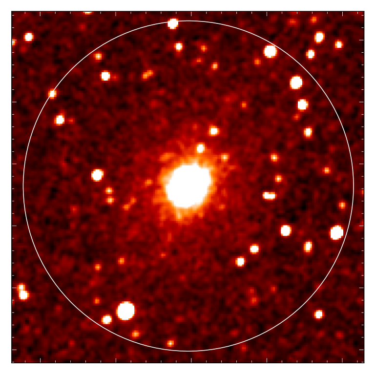
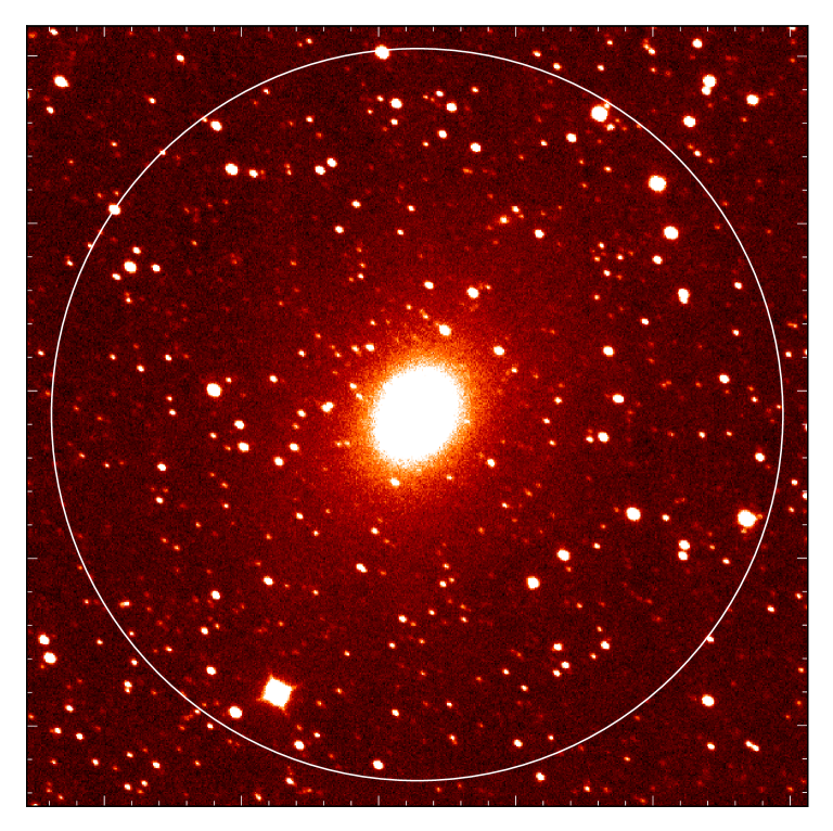
Figure 3: Images of one of the Norma cluster galaxies in our FP sample; WKK 6318, from 2MASS (left panel) and ESO/NTT (right panel).

3 Photometry data analysis

The FP is the relationship between two photometric parameters (that is, the effective radius, $r_{e}$ and the mean surface brightness within that radius, $\langle\mu_{e}\rangle$ ), and the central velocity dispersion. In this section we describe the methods adopted to determine $r_{e}$ and $\langle\mu_{e}\rangle$. The Norma cluster is located close to the galactic plane where stellar contamination is severe and therefore special techniques were needed to reliably subtract the foreground stars.

3.1 Star-subtraction

Star-subtraction was performed using a script that employs various Iraf tasks mostly from the Iraf package Daophot (Stetson, 1987). Figure 4 shows one of the images in our sample before and after star-subtraction (left and right panel, respectively).

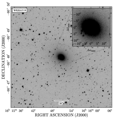
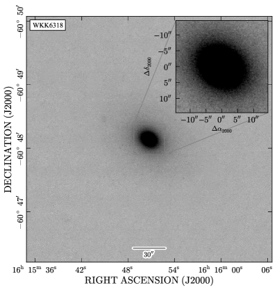
Figure 4: Star-subtraction – WKK 6318. The left panel shows the original image while the right panel shows the corresponding image after star-subtraction.

We have performed a thorough analysis to investigate the effect of our star-subtraction algorithm on our photometry for the Norma cluster. To quantify this effect, a simulation was performed using 12 ETGs from the Centaurus cluster. The choice of the Centaurus galaxies was motivated by the low stellar density. In the simulation, stars from a typical, randomly selected Norma field were added to the Centaurus galaxies. Photometric analysis was performed both before adding and after subtracting the superimposed stars. We found a small correction with a mean value of $\bigtriangleup\text{m}=-0\!\mbox{$\;\mathrm{.}\!\!^{\textrm{m}}$}0106\pm 0\!\mbox{$\;\mathrm{.}\!\!^{\textrm{m}}$}0003$ (see Fig. 9). We apply this value to correct the measured galaxy magnitudes for star-subtraction effects.

3.2 Sky background estimation

For accurate photometry, a reliable estimate of the sky background is crucial – over-estimating the sky value results in galaxies appearing fainter than they are, and vice-versa. We have determined the sky background within an annulus and measured the median sky value. The width of the annulus varied according to the initial estimate of the galaxy size, i.e., we approximated the galaxy size to be $\sim$ three times the measured effective radius ($r_{e}$) and set the inner and outer radii to $3.5\,r_{e}$ and $6\,r_{e}$, respectively. In cases (only for the Coma 2MASS images) where the outer radius ($6\,r_{e}$) is greater than the image size, the outer radius was set to match the image size but excluded the pixels on the edges. To minimise the effect of unresolved stars and other major artefacts, we iteratively applied a $2\sigma_{s}$ clipping where $\sigma_{s}$ is the standard deviation in the sky background within the annulus used. This effectively narrows down the effect of outliers at both the lower- and higher-ends of the pixel-value distribution. The resulting distribution is Gaussian in nature with the median sky value $\approx$ mean sky value.

3.3 Determination of total magnitudes: surface brightness profile fitting

Galaxy surface brightness profiles are usually fitted using a simple Sérsic (Sersic, 1968) profile. In flux units, the single Sérsic component takes the form:

$$I(r)=I_{0}\exp\displaystyle{\left[-\left(\dfrac{r}{r_{0}}\right)^{\frac{1}{n}}\right]}.$$ (2)

$I_{0}$ refers to the central intensity, $r_{0}$ is the scaling radius, $n$ is the Sérsic index, also known as the concentration or shape parameter. Special surface brightness profiles, where $n$ $=$ $0.5$, $n$ $=$ $1$, $n$ $=$ $4$ are referred to as Gaussian, exponential and de Vaucouleurs profiles, respectively. In units of magnitudes, Eq. 2 can be expressed in the form:

$$\mu(r)=\mu(r_{0})+1.086\displaystyle{\left[\left(\dfrac{r}{r_{0}}\right)^{\frac{1}{n}}\right]};$$ (3)

where $\mu(r_{0})$ is the central surface brightness in mag arcsec^-2 and $\mu_{e}\propto-2.5\,\log\,I_{e}$.

In our photometric analysis, we have used the Ellipse task under the Stsdas–Analysis–Isophote package in Iraf, to fit isophotes and derive galaxy surface brightness profiles. The resulting surface brightness profiles were then fitted using a combination of two Sérsic functions (see, e.g., Huang et al. 2013) and the total flux was determined by extrapolation. The fitting method was applied to both Coma and Norma samples. Figure 5 is an example of the fitted profiles, for Coma (top) and Norma (bottom). The red solid line represents the best fit (which is the sum of the two Sérsic components), which we extrapolate so as to determine the galaxy flux that would otherwise get lost within the background noise. The data used to fit the galaxy surface brightness profiles for the Norma sample were restricted for the radius ranging from twice the FWHM (indicated by the small dashed vertical lines on the extreme left) to where the galaxy flux is 1$\sigma_{s}$ above the sky background (vertical dashed lines on the extreme right). FWHM and $\sigma_{s}$ are the seeing and sky background deviation for each image, respectively. For the Coma sample, we restricted the data to within an inner radius of 0 $\aas@@fstack{\prime\prime}$5 and an outer radius where the galaxy flux is 1$\sigma_{s}$ above the sky background.

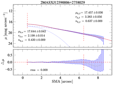
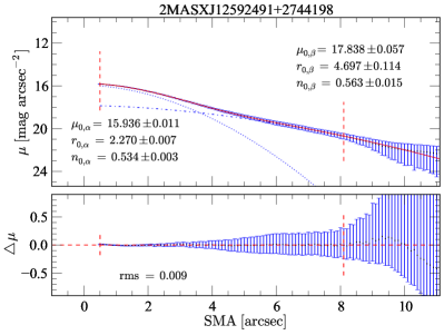
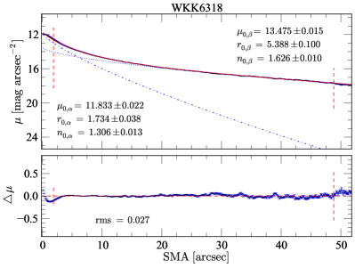
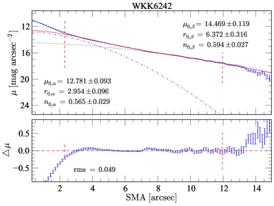
Figure 5: Double Sérsic component fits to the galaxy surface brightness profile for some of the Coma (top left and right panels) and the Norma (bottom left and right panels) cluster galaxies in our sample. The dotted and dot-dashed blue lines represent the individual Sérsic components while the red solid line represents the combined fit. The small dashed vertical line on the extreme left corresponds to a radius twice the seeing (FWHM) for Norma and an inner radius of 0 $\aas@@fstack{\prime\prime}$5 (for the Coma sample). The small dashed vertical line on the far right corresponds to the radius where the galaxy flux is approximately equal to the measured deviation in the sky background – these two small vertical lines represent the range of the data points used to fit the galaxy surface brightness profile. The subscripts $\alpha$ and $\beta$ denote the fit parameters for the two separate Sérsic components which were used to simultaneously fit the galaxy surface brightness profiles. The best fit (solid red curve) is the combination of the two Sérsic components.

The total luminosity, $L_{\rm tot}$ for a single Sérsic component, can be obtained by extrapolating the surface brightness profile to infinity. Within a given radius $r_{\rm max}$, the luminosity, $L_{r_{\rm max}}$ is given by integrating the galaxy profile to the given radius.

$$L_{tot} = \displaystyle{\int_{0}^{\infty}2\pi rI(r)\,\mathrm{d}r}=2\pi I_{0}\,n\,{r_{0}}^{2}\,\Gamma(2n);$$ (4)

$$L_{r_{max}} = \displaystyle{\int_{0}^{r_{max}}2\pi rI(r)\,\mathrm{d}r};$$ (5)

$$= 2\pi I_{0}\,n\,{r_{0}}^{2}\,\displaystyle{\gamma\left[2n,\,\left(\dfrac{r_{max}}{r_{0}}\right)^{1/n}\right]};$$

where $\Gamma(x)$ and $\gamma(s,x)$ are the complete and incomplete gamma functions, respectively. For a double Sérsic profile, the total luminosity for the galaxy is computed by combining the two components. To recover the galaxy flux in the outer parts that would otherwise get lost within the background noise, we apply:

$$L_{\rm{tot}}=L\left(r=r_{\rm{max}}\right)+L\left(r_{\rm{max}}<r<r_{\infty}\right).$$ (6)

3.4 Effective radius and PSF correction

The effective (half-light) radius for each galaxy was measured from the circle enclosing half the total flux through interpolation. This was then corrected for seeing effects using Galfit (Version 3.0.5; Peng et al., 2010) following the description in Magoulas et al. (2012), i.e., we used Galfit to model the galaxy images with and without PSF convolution. The effective radii were measured from the resulting Galfit models. The difference in the effective radius from the PSF convolved model ($r_{e,\rm{psf}}$) and the model without PSF convolution ($r_{e,\rm{nopsf}}$) is the seeing correction, i.e., $r_{e,\rm{psf}}-r_{e,\rm{nopsf}}$. This was subtracted from the effective radius measured from the original image. The effective surface brightness is computed from the seeing-corrected effective radius (circular) using $\langle\mu_{e}\rangle=m_{{}_{\rm{tot}}}+2.5\,\log(2\pi)+5\,\log r_{e}$; where $m_{{}_{\rm{tot}}}$ is the total extrapolated magnitude corrected for the star-subtraction and sky background effects.

3.5 Measurement errors and analysis

The errors on the effective radius and the total extrapolated magnitude (and hence $\langle\mu_{e}\rangle)$ are correlated. For the Norma cluster sample, we modelled the errors in the photometric parameters using Galfit. Using the Galfit output parameters (total magnitude, effective radius along semi-major axis, axial ratio, position angle, Sérsic index) of the galaxy, we created mock images corresponding to the respective Galfit output parameters for each of the galaxies in our Norma cluster sample. Each of the mock galaxy models was convolved with the PSF image for the respective galaxy field before adding it to the different positions in the original galaxy image field (the data image) but avoiding the centre or the position of the original observed galaxy. Photometry was performed on each of the added fake galaxies and the output is compared with the input parameters. The difference between the simulated and true magnitude is negligible, with a median value of $-0\!\mbox{$\;\mathrm{.}\!\!^{\textrm{m}}$}008$. This indicates that our photometry is not significantly affected by sky gradients or faint unresolved stars in the field. By using the median value for each individual galaxy field, the measurement error on the total magnitude from the simulation is $\sim$ 0​$\;\mathrm{.}\!\!^{\textrm{m}}$02 $\pm$ 0​$\;\mathrm{.}\!\!^{\textrm{m}}$01. In addition, we measured the magnitude error within an aperture whose size is four times the measured effective radius (taking into consideration the photometric zero-points error as well). The total error on the total extrapolated magnitude is the quadrature sum of the error obtained through the simulation and the aperture photometry error within the 4​ $r_{e}$ apertures. The measurement errors on the total magnitude for the 2MASS Coma cluster galaxies were determined following the description given in the 2MASS All-Sky Data Release Explanatory Supplement (see http://www.ipac.caltech.edu/2mass/releases/allsky/doc/sec6_8a.html). The error on the total magnitude was calculated using:

$$\bigtriangleup\rm{mag}=1.087\,\dfrac{\left[\left(S/g_{\rm{av}}\right)+n\left(2k\sigma_{s}\right)^{2}+\left(0.024n\sigma_{s}\right)^{2}\right]^{1/2}}{S};$$ (7)

where $g_{\rm{av}}=G\times N$ where $G=10$ is the gain, $N=6$ is the total number of co-added frames, $S$ is the total flux, $k\approx 1.7$ is the Kernel smoothing factor, $\sigma_{s}$ is the co-added noise, and $n$ is the total number of pixels within an aperture. We used a size of aperture equal to four times the effective radius, so that the aperture magnitude within that radius would be a good approximation to the measured galaxy total extrapolated magnitude.

For both Norma and Coma sample galaxies, we measured the corresponding error in the effective radius (arising from the error in the total magnitude), and applied simple propagation of errors to compute the error in the mean effective surface brightness.

Table 3: Corrections and systematic errors for the Norma ETGs. The extinction correction presented in this table is from SF11 (refer to section 3.6.1 for details).

	Correction	Error	S/M
(1)	(2)	(3)	(4)
Star-subtraction [mag]	$-$0.0106	0.0003	M
Sky background [mag]	$-$0.008	0.020	M
Photometric calibration [mag]	-	0.025	S
$\sigma$-aperture correction [dex]	$-$0.015	-	M
$\sigma$-run offset [dex]	0.012	0.007	M
Malmquist bias [%]	0.587	-	S
Extinction correction [mag]	0.057 – 0.088	-	S
$k$-correction [mag]	0.042 – 0.071	-	S
Seeing correction [′′]	0.001 – 2.607	-	M
Cosmological dimming [mag]	0.051 – 0.091	-	S

Column 1 represents the different corrections applied to the spectroscopic and photometric measurements for the Norma sample. Column 2 is the mean value of the correction. Where the correction was applied to individual galaxies, the range is given. Column 3 is the error on the mean value. M and S given in Column 4 refer to the type, i.e., measurement and systematic errors, respectively.

An independent photometric analysis was performed on the Coma sample, where the effective radius for each galaxy was measured based on the galaxy’s total extrapolated magnitude from the 2MASS Extended Source Catalogue (Jarrett et al., 2000; Skrutskie et al., 2006). There is a small offset (median value) of $0\!\mbox{$\;\mathrm{.}\!\!^{\textrm{m}}$}014\pm 0\!\mbox{$\;\mathrm{.}\!\!^{\textrm{m}}$}009$ between these measurements and ours, with 2MASS magnitudes being brighter. The median difference in the X-component of the FP (i.e., $\log\,r_{e}-0.32\langle\mu_{e}\rangle$), between our results and the independent measurements, is $-0.005\pm 0.001$ dex.

3.6 Photometric corrections to $\mn@boldsymbol{\langle\mu_{e}\rangle}$ and systematics

3.6.1 Galactic extinction corrections

The effect of galactic extinction can be corrected for using the DIRBE/IRAS reddening maps of Schlegel, Finkbeiner & Davis (1998). It has been found however, that the Schlegel et al. NIR reddening maps, over-estimate the extinction at low Galactic latitudes where they are uncalibrated – see, e.g., Bonifacio et al. (2000); Schröder et al. (2007); Schlafly & Finkbeiner (2011). For our analysis, we adopt the correction factor of 0.86 by Schlafly & Finkbeiner (2011) which is a modification of the Schlegel et al. maps. We used NED to extract the Schlafly & Finkbeiner (2011) extinctions in the Landolt $B$-band and converted them to the $K_{s}$-band using $A_{K_{s}}=0.085\,A_{B}$. The extinction values for the Norma sample range from 0.057 to 0.088 mag (see Table 3.5). The mean difference due to the modification is, on average, 0​$\;\mathrm{.}\!\!^{\textrm{m}}$011, which corresponds to a Norma distance offset of 45 km s^-1.

3.6.2 Redshift and cosmological dimming corrections to $\langle\mu_{e}\rangle$

We applied a $k$-correction, $k_{K_{s}}=-3.83z+21.9z^{2}$, as given by Pahre (1999). Various redshift corrections exist, e.g., Bell et al. (2003) gives a $k$-correction of $-2.1z$. Applying this correction results in a magnitude difference of $0\!\mbox{$\;\mathrm{.}\!\!^{\textrm{m}}$}02$ and $0\!\mbox{$\;\mathrm{.}\!\!^{\textrm{m}}$}03$ for the Norma and Coma clusters, respectively. The corresponding distance offset for Norma is $\sim$ 33 km s^-1.

The cosmological dimming effect on the mean effective surface brightness, which is due to uniform expansion of space was corrected for, using the $(1+z)^{4}$ term – the cosmological dimming correction term is $-10\log\,(1+z)$. At the redshift distances of Norma and Coma, the mean corrections are 0.07 mag arcsec^-2 and 0.10 mag arcsec^-2, respectively.

3.7 Fundamental Plane data: $\mn@boldsymbol{\log r_{e}}$, $\mn@boldsymbol{\langle\mu_{e}\rangle}$ and $\mn@boldsymbol{\log\sigma}$

The FP relates the stellar properties (central velocity dispersion, $\sigma$), galaxy size (effective radius, $r_{e}$), and the mean galaxy surface brightness within the effective radius ($\langle\mu_{e}\rangle$) of ETGs, i.e.,

$$\log r_{e}=a\log\sigma+b\langle\mu_{e}\rangle+c;$$ (8)

where $a$ and $b$ are the FP slopes, while $c$ is the intercept (zero-point). The fully corrected mean effective surface brightness ($\langle\mu_{e}\rangle$) that is finally used in fitting the FP is

$$\langle\mu_{e}\rangle=m_{\rm{tot}}+2.5\log\left(2\pi r^{2}_{e}\right)-A_{K_{s}}+k_{K_{s}}-10\log\left(1+z\right);$$ (9)

where $m_{\rm{tot}}$ is the measured total extrapolated apparent magnitude. Table 4 shows the results for the Norma cluster sample. Included in the table are the final variables ($r_{e}$, $\langle\mu_{e}\rangle$, and $\log\sigma$) used to fit the FP. A similar table for the Coma cluster sample is provided in the appendix (refer to Table 6).

Table 4: Norma cluster photometry results obtained by fitting and extrapolating the galaxy surface brightness profiles.

Identification	Tot. mag	$r_{e}$	$\langle\mu_{e}\rangle$	$A_{{}_{K_{s}}}$	$z_{{}_{\rm{helio}}}$	$\log\sigma$
(1)	(2)	(3)	(4)	(5)	(6)	(7)
WKK5920	9.93$\pm$0.04	4.63$\pm$0.43	15.03$\pm$0.21	0.086	0.0159	2.312$\pm$0.012
WKK5972	9.64$\pm$0.05	6.72$\pm$0.76	15.54$\pm$0.25	0.079	0.0185	2.414$\pm$0.010
WKK6012	10.89$\pm$0.05	4.48$\pm$0.38	15.94$\pm$0.19	0.080	0.0146	2.172$\pm$0.014
WKK6019	9.94$\pm$0.04	3.72$\pm$0.26	14.56$\pm$0.15	0.070	0.0186	2.409$\pm$0.010
WKK6047	11.90$\pm$0.07	3.07$\pm$0.21	16.11$\pm$0.16	0.070	0.0180	2.010$\pm$0.015
WKK6116	9.39$\pm$0.03	6.66$\pm$0.56	15.33$\pm$0.19	0.066	0.0129	2.344$\pm$0.012
WKK6180	10.15$\pm$0.05	6.07$\pm$0.59	15.87$\pm$0.22	0.065	0.0153	2.308$\pm$0.011
WKK6183	10.30$\pm$0.04	4.35$\pm$0.30	15.27$\pm$0.16	0.063	0.0198	2.377$\pm$0.012
WKK6198	11.71$\pm$0.09	4.29$\pm$0.58	16.67$\pm$0.31	0.056	0.0158	1.905$\pm$0.020
WKK6204	9.39$\pm$0.04	6.58$\pm$0.64	15.28$\pm$0.21	0.065	0.0154	2.499$\pm$0.009
WKK6221	10.70$\pm$0.06	6.44$\pm$0.48	16.51$\pm$0.17	0.066	0.0195	2.038$\pm$0.017
WKK6229	11.59$\pm$0.04	1.92$\pm$0.07	14.78$\pm$0.09	0.063	0.0177	2.210$\pm$0.015
WKK6233	11.77$\pm$0.06	2.36$\pm$0.16	15.42$\pm$0.16	0.062	0.0171	2.243$\pm$0.014
WKK6235	10.95$\pm$0.05	3.31$\pm$0.30	15.36$\pm$0.21	0.069	0.0135	2.141$\pm$0.018
WKK6242	10.92$\pm$0.03	2.09$\pm$0.09	14.31$\pm$0.10	0.061	0.0175	2.424$\pm$0.011
WKK6250	10.47$\pm$0.04	3.18$\pm$0.24	14.74$\pm$0.17	0.064	0.0206	2.324$\pm$0.010
WKK6269	8.27$\pm$0.05	15.95$\pm$1.44	16.07$\pm$0.20	0.060	0.0182	2.579$\pm$0.011
WKK6282	11.23$\pm$0.04	1.56$\pm$0.17	14.00$\pm$0.24	0.060	0.0165	2.274$\pm$0.012
WKK6305	9.15$\pm$0.04	8.05$\pm$0.61	15.45$\pm$0.17	0.080	0.0165	2.327$\pm$0.009
WKK6318	8.70$\pm$0.06	15.52$\pm$1.46	16.48$\pm$0.21	0.073	0.0114	2.354$\pm$0.013
WKK6342	11.04$\pm$0.03	2.39$\pm$0.06	14.72$\pm$0.06	0.062	0.0162	2.326$\pm$0.009
WKK6360	10.11$\pm$0.02	3.14$\pm$0.08	14.35$\pm$0.06	0.063	0.0208	2.505$\pm$0.009
WKK6383	10.95$\pm$0.05	4.00$\pm$0.27	15.74$\pm$0.15	0.071	0.0185	2.195$\pm$0.012
WKK6431	10.87$\pm$0.03	2.50$\pm$0.16	14.68$\pm$0.14	0.075	0.0118	2.286$\pm$0.010
WKK6473	11.94$\pm$0.07	2.00$\pm$0.16	15.23$\pm$0.19	0.067	0.0186	2.064$\pm$0.017
WKK6477	11.84$\pm$0.06	2.69$\pm$0.21	15.79$\pm$0.18	0.073	0.0135	2.106$\pm$0.019
WKK6555	11.04$\pm$0.06	2.79$\pm$0.38	15.05$\pm$0.30	0.067	0.0165	2.207$\pm$0.010
WKK6600	10.07$\pm$0.05	5.15$\pm$0.58	15.41$\pm$0.25	0.068	0.0168	2.338$\pm$0.011
WKK6615	12.04$\pm$0.08	2.22$\pm$0.21	15.59$\pm$0.22	0.060	0.0139	2.108$\pm$0.021
WKK6620	12.94$\pm$0.21	2.83$\pm$0.56	16.97$\pm$0.48	0.062	0.0208	1.777$\pm$0.054
WKK6679	10.79$\pm$0.04	3.19$\pm$0.20	15.10$\pm$0.14	0.074	0.0155	2.159$\pm$0.012

NOTES: The columns refer to (1) galaxy name (2) the measured total extrapolated magnitude corrected for the star-subtraction and background effects (3) effective radius in arcsec corrected for the seeing effect (4) mean effective surface brightness in $\rm{mag}\;\rm{arcsec}^{-2}$, corrected for galactic extinction, redshift, and the cosmological dimming effects (5) galactic extinction from SF11: $A_{K_{s}}=0.085\,A_{B}$ (6) galaxy redshift (heliocentric) (7) central velocity dispersion in dex, with both aperture correction and run offset applied.

4 Relative distance between Norma and Coma

4.1 Fitting the Fundamental Plane

The FP relation (or the closely equivalent D_n-$\sigma$ relation) has been widely used to determine the relative distances of ETGs and measure peculiar velocities, e.g., (Lynden-Bell et al., 1988; Lucey & Carter, 1988), SMAC (Hudson et al., 1999, 2004), ENEAR (da Costa et al., 2000), EFAR (Colless et al., 2001), 6dFGSv (Magoulas et al., 2012).

We have used the Coma cluster for calibration. To minimise the effect of sample selection biases and the effect of outliers, we fitted for the FP parameters by minimising the absolute residuals along the $\log\sigma$ direction (Strauss & Willick, 1995; Jorgensen et al., 1996; La Barbera et al., 2010). Simultaneous least-squares fitting was used by constraining the FP parameters $a$ and $b$ to be the same for both Norma and Coma, while we allowed the FP intercepts to vary between the two clusters.

Our FP fit parameters are $a=1.465\pm 0.059$, $b=0.326\pm 0.020$, with an rms scatter of $\sim$ 0.08 dex in $\log\sigma$. The zero-point offset is $0.154$ $\pm$ $0.014$. Figure 6 shows the projected FP. The Norma cluster which is represented by the red filled circles has been shifted to the Coma distance.

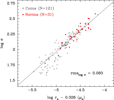
Figure 6: $K_{s}$-band FP projection, obtained by simultaneously minimising absolute residuals along $\log\sigma$; for the Coma cluster (open circles), and the Norma cluster (red filled circles). The Norma cluster has been shifted by applying the FP offset so that it lies at the Coma distance.

The error in individual galaxy distances is $\Delta_{g}=a\ln(10)\Delta_{\sigma}$. For cluster distances, the percentage error reduces according to the number of galaxies ($N$) in the sample, and is given by $\Delta_{g}/\sqrt{N}$. However, one needs to correct for the effect of Malmquist bias. The homogeneous Malmquist bias increases with distance but also decreases with the number of galaxies in the sample. For a measured distance $d$, the distance corrected for the homogeneous Malmquist bias is given by $d\exp(3.5\Delta_{g}^{2}/N)$ (Hudson et al., 1997). The correction is thus 0.59% ($\sim$ 29 km s^-1 at the Norma distance).

4.2 The MIST algorithm

For comparison, we have fitted the FP using the Measurement errors and Intrinsic Scatter Three dimensional (MIST) algorithm kindly provided by La Barbera, Busarello & Capaccioli (2000). The MIST algorithm is a bisector least-squares fit, used to determine the FP parameters $a$, $b$, and $c$. The statistical errors on the FP coefficients are computed through an inbuilt bootstrap analysis. For the MIST algorithm, we fitted the Coma FP (along $\log\sigma$-direction) and fixed the slopes $a$ and $b$ to determine the median value of the intercept, $c_{{}_{\rm N}}$ for the Norma cluster. The FP zero-point offset measured using this method is $0.154$ $\pm$ $0.019$.

While low velocity dispersion galaxies have larger measurement errors (see Fig. 10), we found no significant change in the derived Norma distance as a result of including these low velocity dispersion galaxies in our FP analysis. Through a bootstrap analysis (using the Coma ETGs), we analysed the change in the FP fit parameters with and without a magnitude cut. We applied a magnitude cut of 12​$\;\mathrm{.}\!\!^{\textrm{m}}$5 as this effectively excludes most of the Coma ETGs with $\log\sigma<2$ (see Section B). The bootstrap results (FP fit parameters) are shown in Fig. 11.

4.3 Fixed metric aperture magnitudes: the modified Faber–Jackson relation

Relative distances can also be measured using the Faber-Jackson (FJ) relation (Faber & Jackson, 1976) with galaxy magnitudes determined within a fixed metric radius (Lucey, 1986). This approach bypasses the uncertainties that arise from the determination of total magnitudes and allows relative distances to be measured to a similar accuracy to the FP. We have applied this technique as an alternative way to determine the Norma-Coma relative distance.

To make the PSF-corrections to the aperture photometry managable, we adopt a metric radius of 2 kpc which corresponds, for our Coma cluster distance, to an aperture radius of 4 $\aas@@fstack{\prime\prime}$16. Galfit was used to determine the PSF-corrected aperture magnitudes for all galaxies in our Coma sample. For each galaxy in the Norma sample we determined a set of PSF-corrected aperture magnitudes that spanned a range of possible Norma cluster distances; if Norma has zero peculiar velocity then the 2 kpc radius corresponds to a size of 5 $\aas@@fstack{\prime\prime}$99. Galactic extinction and k-corrections were applied.

A least-squares fit, minimising in the $\log\sigma$ direction, was used to simultaneously determine the slope of the combined L(r = 2 kpc) – $\sigma$ relation and the relative Norma-Coma offset. A range of Norma-Coma offsets were considered and for each the appropriate aperture size (i.e., based on the assumed relative Norma-Coma distance) was used for the Norma photometry. The best-fit was taken to be where there was no systematic difference in the L(r = 2 kpc) – $\sigma$ relation between the two clusters and this corresponds to an offset of $0.159$ $\pm$ $0.022$ dex (see Fig. 7). This derived value is in very good agreement with that directly determined from the FP analysis.

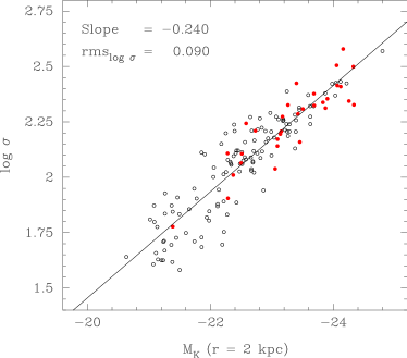
Figure 7: The FJ relation, based on aperture photometry using an aperture radius equal to 2 kpc. The black open circles represent the Coma cluster, the red filled circles are from the Norma cluster.

5 The distance and peculiar velocity of the Norma cluster

The measured Norma-Coma offsets derived from the three different methods presented in Section 4 are in excellent agreement, i.e., 0.154 $\pm$ 0.014, 0.154 $\pm$ 0.019, 0.159 $\pm$ 0.022. For our following analysis we adopt the offset from the simultaneous least-squares fit which has the smallest measurement error. This offset is directly related to the difference in the angular diameter distances (${D_{A}}$) of the two clusters, i.e.,

$$\log{D_{A}\left(\rm{Coma}\right)}-\log{D_{A}\left(\rm{Norma}\right)}=0.154\,\pm\,0.014.$$ (10)

In our analysis we assume that the Coma cluster has zero peculiar velocity and hence Coma’s Hubble flow redshift, $z_{{}_{\rm{H}}}$, is equal to the observed redshift in the local CMB rest frame, $z_{{}_{\rm{CMB}}}$. For our adopted cosmology and a Coma CMB redshift ($z_{{}_{\rm{CMB}}}$) of 0.02400 $\pm$ 0.00016 then $\log{D_{A}\left(\rm{Coma}\right)}$ = 1.996 $\pm$ 0.003 where the angular diameter distance is given in Mpc. Hence we find $\log{D_{A}\left(\rm{Norma}\right)}$ = 1.842 $\pm$ 0.014 which implies a Hubble flow redshift for Norma ($z_{{}_{\rm{H}}}$) of 0.01667  $\pm$  0.00055.

We derived Norma’s peculiar velocity redshift, $z_{{}_{\rm PEC}}$, via ( 1 + z__CMB) = ( 1 + z__H)( 1 +z__PEC) (Harrison, 1974). Norma’s redshift in the local CMB rest frame, $z_{{}_{\rm CMB}}$, is 0.01652 $\pm$ 0.00018. Hence we derived a value for Norma’s peculiar velocity of –43 $\pm$ 170 km s^-1. Adding in the homogeneous Malmquist bias correction (see Section 4.1) lowers this value to –72  km s^-1. Hence, we find that the Norma cluster has a small and insignificant peculiar velocity of –72 $\pm$ 170 km s^-1.

All-sky galaxy redshift surveys map the local cosmography and allow reconstructions of the density field (and the peculiar velocity field) to be made. The reconstruction of the IRAS Point Source Catalogue redshift survey (PSCz, Saunders et al., 2000) by Branchini et al. (1999) provides a data cube of the predicted peculiar velocity components $v_{x}$, $v_{y}$ and $v_{z}$ at grid positions $x$, $y$, $z$. Lavaux et al. (2010)’s predictions derived from the 2MASS Redshift Survey (Huchra et al., 2012) are available at the Extragalactic Distance Database (Tully et al., 2009). We have used these two reconstructions to estimate the peculiar velocity in the Norma line-of-sight direction (see Fig. 8). The PSCz reconstruction under-estimates the peculiar velocities as compared to the 2MRS reconstruction possibly due to the former being less sensitive to galaxy clusters (Branchini, private communication). Both these studies predict a small peculiar velocity for Norma, i.e., less than $\pm$ 100 km s^-1, which is in good agreement with our measurement of –72 $\pm$ 170 km s^-1.

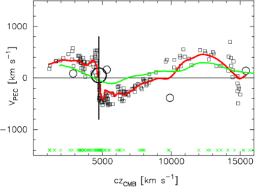
Figure 8: Model predictions for the peculiar velocity in the Norma cluster direction. The green and red curves represent PSCz and 2MRS predictions, respectively. The crosses shown at the bottom of each panel show the redshifts of the PSCz galaxies in the cone. The black squares show the 2MRS predictions. The squares are non-grouped galaxies while the circles represent groups with the size of the circle reflecting the number of galaxies in the group. Norma is the large bold circle.

In Table 3.5, we presented a summary of possible sources of measurement and systematic errors and the applied corrections. We found through simulations, that the effect of star-subtraction is very small, $\sim$ $0\!\mbox{$\;\mathrm{.}\!\!^{\textrm{m}}$}011$ which translates into a distance offset of $\sim$ 44 km s^-1. The systematic effects arising from possible gradients in the sky background and non-resolved stars are very small, i.e., $\sim$ 32 km s^-1. For extinction corrections, the correction factor ranges from 70% to 90% (e.g., Bonifacio et al. 2000; Yasuda et al. 2007; Schröder et al. 2007; Schlafly & Finkbeiner 2011) which implies an uncertainty in distance in the range of –63 km s^-1 to 16 km s^-1. Note also that a $\pm$ 100 km s^-1 peculiar velocity for Coma would change our value for Norma by $\pm$ 69 km s^-1.

6 Discussion and conclusions

The GA is now widely identified as the Hydra-Cen-Norma supercluster (Courtois et al., 2012; Shaya & Tully, 2013; Tully et al., 2013). Since the original discovery of the large positive peculiar velocities in the Hydra-Centaurus region (Lynden-Bell et al., 1988), new measurements, particularly for clusters, in the general GA region have been made. In Table 5 we summarise the results from the FP-based SMAC and ENEARc surveys, the Tully-Fisher SFI++ survey and our Norma measurement. Although the typical measurement errors are between 150 and 400 km s^-1, most GA clusters are observed to have positive peculiar velocities with an “average” value of $\sim$+300 km s^-1.

Our peculiar velocity measurement of –72 $\pm$ 170 km s^-1 for the Norma cluster is lower than most values found for other GA clusters and hence may indicate that Norma lies close to the GA’s “core”. The uncertainties on the cluster peculiar velocities listed in Table 5 are sufficiently large that we can not currently determine whether or not Norma partakes in the general GA outflow. However there is strong independent support for the GA outflow from the Type Ia supernovae data (see Lucey et al. 2005) and many studies (e.g., Hudson et al. 1999) have attributed a major part of this large scale outflow to the Shapley Supercluster that lies $\sim$10 000 km s^-1 more distant in this general direction. Bolejko & Hellaby (2008) estimate that Shapley can cause the GA to have a net peculiar velocity of $\sim$ +80 km s^-1.

While our knowledge of the local cosmography in the GA direction has improved considerably from galaxy redshift surveys that probe close to the galactic plane (Radburn-Smith et al., 2006; Jones et al., 2009; Huchra et al., 2012), there are still aspects that are incomplete and some important clusters/groups belonging to the GA may still remain hidden. An example is the discovery of CIZA J1324.7-5736 (Ebeling, Mullis & Tully, 2002), the second richest cluster in the GA region (Nagayama et al., 2006). Dedicated surveys are now underway to map larger swaths of the local universe veiled by the Milky Way, including ground-based near-IR surveys (see, e.g., Kraan-Korteweg et al., 2011), and in the mid-IR using WISE (Bilicki et al., 2014; Jarrett et al., 2013) and in the radio by targeting neutral hydrogen, notably with HIPASS and HIZOA (Henning et al., 1999; Henning et al., 2000; Kraan-Korteweg et al., 2000; Schröder et al., 2009). Judicious application of the mid-infrared Tully-Fisher relation is now being considered to study the peculiar motions of gas-rich galaxies in massive structures that inhabit or cross the ZoA (Sorce et al., 2012; Lagattuta et al., 2013; Said, 2013). And our study of Norma has demonstrated that, despite the challenges of the large galactic extinction and severe stellar contamination, FP distances can be derived reliably for ETGs that lie relatively close to the galactic plane. The exploitation of such techniques will be essential to gain a more complete understanding of the GA and other important large scale structures that comprise the hidden cosmic web.

Table 5: Peculiar velocities of Clusters/Groups in the GA region. $N_{\phi}$ is the angle on the sky between the cluster and Norma. SMAC measurements from Hudson et al. (2004), SFI++ measurements from Springob et al. (2007), ENEARc measurements from Bernardi et al. (2002).

Cluster	$\ell$	$b$	$N_{\phi}$	cz${}_{{}_{\rm CMB}}$	N	$v_{{}_{\rm PEC}}$	Source
	∘	∘	∘	km s-1		km s-1
A1060 (Hydra)	270	26	62	4055	26	+254 $\pm$ 223	SMAC
					39	–47 $\pm$ 168	ENEARc
					21	–422 $\pm$ 169	SFI++
AS636 (Antlia )	272	19	58	3129	17	+292 $\pm$ 102	SFI++
AS639	281	11	47	6526	6	+1615 $\pm$ 453	ENEARc
N3557 group	282	21	50	3318	7	+281 $\pm$ 160	SFI++
A3526A (Cen30)	302	22	37	3300	27	+351 $\pm$ 136	SMAC
					21	+500 $\pm$ 153	ENEARc
					23	+260 $\pm$ 124	SFI++
AS714	303	36	47	3576	7	+559 $\pm$ 245	ENEARc
A3537	305	31	43	5370	4	+482 $\pm$ 560	SMAC
CIZA J1324.7-5736	308	5	21	5899
E508 group	309	39	48	3310	9	+382 $\pm$ 122	SFI++
A3574 (K27)	317	31	39	4881	8	+487 $\pm$ 351	SMAC
					10	+479 $\pm$ 310	ENEARc
					13	–199 $\pm$ 210	SFI++
AS753	319	26	34	4431	14	+376 $\pm$ 282	SMAC
					18	+812 $\pm$ 204	ENEARc
A3581	323	33	40	6714	8	+131 $\pm$ 533	SMAC
A3627 (Norma)	325	–7	0	4954	31	–72 $\pm$ 170	This study
AS761	326	32	39	7076	11	+332 $\pm$ 483	SMAC
AS805 (Pavo-II)	332	–23	17	4266	9	+293 $\pm$ 326	SMAC
					12	–18 $\pm$ 268	ENEARc
					8	+304 $\pm$ 147	SFI++
Pavo I group	334	–36	30	4055	16	+473 $\pm$ 191	SFI++

Acknowledgments

TM acknowledges financial support from the Square Kilometre Array South Africa (SKA SA). PAW, SLB, THJ and MB acknowledge financial support from the South African National Research Foundation (NRF) and the University of Cape Town. JRL acknowledges support from STFC via ST/I001573/1. Funding for SDSS-III has been provided by the Alfred P. Sloan Foundation, the Participating Institutions, the National Science Foundation, and the U.S. Department of Energy Office of Science. The SDSS-III web site is http://www.sdss3.org/. SDSS-III is managed by the Astrophysical Research Consortium for the Participating Institutions of the SDSS-III Collaboration including the University of Arizona, the Brazilian Participation Group, Brookhaven National Laboratory, Carnegie Mellon University, University of Florida, the French Participation Group, the German Participation Group, Harvard University, the Instituto de Astrofisica de Canarias, the Michigan State/Notre Dame/JINA Participation Group, Johns Hopkins University, Lawrence Berkeley National Laboratory, Max Planck Institute for Astrophysics, Max Planck Institute for Extraterrestrial Physics, New Mexico State University, New York University, Ohio State University, Pennsylvania State University, University of Portsmouth, Princeton University, the Spanish Participation Group, University of Tokyo, University of Utah, Vanderbilt University, University of Virginia, University of Washington, and Yale University. This publication has made use of the NASA/IPAC Extragalactic Data base (NED), and also data products from the 2MASS, a joint project of the University of Massachusetts and the Infrared Processing and Analysis Center California Institute of Technology, funded by the National Aeronautics and Space Administration and the National Science Foundation.

Appendix A Photometric analysis

Table 6 represents the ETGs in the Coma sample. No corrections have been applied to the total magnitudes presented in the table.

Table 6: Coma cluster photometry results from fitting and extrapolating the galaxy surface brightness profiles.

Identification	Tot. mag	$r_{e}$	$\langle\mu_{e}\rangle$	$z_{{}_{\rm{helio}}}$	$\log\sigma$
(1)	(2)	(3)	(4)	(5)	(6)
2MASXJ13023273+2717443	13.48$\pm$0.15	3.23$\pm$0.59	17.83$\pm$0.42	0.0254	1.709$\pm$0.055
2MASXJ13020552+2717499	13.51$\pm$0.14	2.21$\pm$0.52	17.04$\pm$0.53	0.0243	1.836$\pm$0.033
2MASXJ13000623+2718022	12.82$\pm$0.07	4.46$\pm$0.46	17.86$\pm$0.23	0.0263	1.748$\pm$0.038
2MASXJ12593730+2720097	14.27$\pm$0.24	2.29$\pm$0.58	17.89$\pm$0.60	0.0233	1.640$\pm$0.076
2MASXJ13010615+2723522	13.83$\pm$0.17	2.15$\pm$0.41	17.28$\pm$0.45	0.0271	1.809$\pm$0.041
2MASXJ12564777+2725158	13.48$\pm$0.12	2.24$\pm$0.27	17.03$\pm$0.29	0.0259	1.618$\pm$0.042
2MASXJ12583209+2727227	12.57$\pm$0.05	1.87$\pm$0.20	15.74$\pm$0.23	0.0234	2.056$\pm$0.014
2MASXJ12573614+2729058	12.15$\pm$0.04	2.05$\pm$0.04	15.52$\pm$0.06	0.0241	2.210$\pm$0.009
2MASXJ12570940+2727587	11.16$\pm$0.02	3.02$\pm$0.02	15.37$\pm$0.02	0.0249	2.304$\pm$0.008
2MASXJ13002689+2730556	12.52$\pm$0.05	2.40$\pm$0.21	16.21$\pm$0.20	0.0260	2.023$\pm$0.014
2MASXJ12580974+2732585	13.28$\pm$0.10	2.95$\pm$0.27	17.45$\pm$0.22	0.0233	1.727$\pm$0.042
2MASXJ12573584+2729358	10.90$\pm$0.02	3.57$\pm$0.02	15.47$\pm$0.02	0.0244	2.321$\pm$0.009
2MASXJ12572435+2729517	9.07$\pm$0.00	21.19$\pm$0.20	17.51$\pm$0.02	0.0245	2.431$\pm$0.008
2MASXJ12570431+2731328	13.63$\pm$0.15	3.17$\pm$0.49	17.92$\pm$0.37	0.0277	1.872$\pm$0.041
2MASXJ12563418+2732200	11.61$\pm$0.03	3.59$\pm$0.07	16.20$\pm$0.05	0.0237	2.208$\pm$0.009
2MASXJ13014841+2736147	12.82$\pm$0.07	2.41$\pm$0.14	16.51$\pm$0.15	0.0275	1.846$\pm$0.022
2MASXJ13011224+2736162	12.53$\pm$0.05	4.37$\pm$0.31	17.53$\pm$0.16	0.0252	1.729$\pm$0.039
2MASXJ13001914+2733135	11.79$\pm$0.03	3.90$\pm$0.24	16.59$\pm$0.14	0.0196	2.030$\pm$0.013
2MASXJ12585812+2735409	12.06$\pm$0.04	2.12$\pm$0.10	15.53$\pm$0.11	0.0200	2.166$\pm$0.011
2MASXJ12573284+2736368	10.62$\pm$0.01	3.76$\pm$0.09	15.33$\pm$0.05	0.0201	2.379$\pm$0.008
2MASXJ13020106+2739109	12.70$\pm$0.07	3.02$\pm$0.24	16.91$\pm$0.19	0.0236	1.805$\pm$0.026
2MASXJ13015375+2737277	10.05$\pm$0.01	5.49$\pm$0.07	15.54$\pm$0.03	0.0262	2.423$\pm$0.008
2MASXJ12591030+2737119	12.34$\pm$0.05	2.75$\pm$0.25	16.38$\pm$0.20	0.0191	2.078$\pm$0.014
2MASXJ12571682+2737068	12.48$\pm$0.05	1.18$\pm$0.33	14.64$\pm$0.61	0.0242	2.208$\pm$0.009
2MASXJ12594713+2742372	11.14$\pm$0.02	3.66$\pm$0.04	15.74$\pm$0.03	0.0280	2.130$\pm$0.010
2MASXJ12584742+2740288	11.07$\pm$0.02	6.77$\pm$0.11	17.00$\pm$0.04	0.0280	2.273$\pm$0.009
2MASXJ12583157+2740247	12.90$\pm$0.07	1.80$\pm$0.15	15.99$\pm$0.20	0.0231	2.104$\pm$0.012
2MASXJ12563420+2741150	13.82$\pm$0.21	2.09$\pm$0.53	17.24$\pm$0.59	0.0229	1.798$\pm$0.029
2MASXJ13000626+2746332	11.98$\pm$0.04	4.21$\pm$0.15	16.94$\pm$0.09	0.0206	2.061$\pm$0.013
2MASXJ12592491+2744198	12.27$\pm$0.04	1.96$\pm$0.13	15.58$\pm$0.15	0.0201	2.159$\pm$0.012
2MASXJ12591348+2746289	11.90$\pm$0.03	3.41$\pm$0.11	16.38$\pm$0.08	0.0228	2.071$\pm$0.014
2MASXJ12590821+2747029	11.13$\pm$0.02	3.45$\pm$0.08	15.63$\pm$0.06	0.0234	2.314$\pm$0.009
2MASXJ12590745+2746039	11.98$\pm$0.04	2.25$\pm$0.06	15.56$\pm$0.07	0.0212	2.223$\pm$0.010
2MASXJ12585766+2747079	13.12$\pm$0.09	3.41$\pm$0.37	17.60$\pm$0.25	0.0231	1.582$\pm$0.055
2MASXJ12585208+2747059	11.65$\pm$0.03	3.34$\pm$0.09	16.11$\pm$0.06	0.0189	2.175$\pm$0.011
2MASXJ12581922+2745437	13.48$\pm$0.13	1.86$\pm$0.40	16.68$\pm$0.49	0.0182	1.872$\pm$0.031
2MASXJ12574616+2745254	12.15$\pm$0.04	5.02$\pm$0.34	17.49$\pm$0.15	0.0204	1.696$\pm$0.042
2MASXJ13011761+2748321	10.88$\pm$0.01	3.69$\pm$0.03	15.53$\pm$0.02	0.0244	2.274$\pm$0.009
2MASXJ13003334+2749266	13.53$\pm$0.12	3.44$\pm$0.31	18.00$\pm$0.23	0.0273	1.625$\pm$0.060
2MASXJ13000551+2748272	11.89$\pm$0.03	3.30$\pm$0.10	16.30$\pm$0.07	0.0219	2.067$\pm$0.013
2MASXJ12595489+2747453	13.74$\pm$0.13	1.47$\pm$0.35	16.36$\pm$0.53	0.0275	1.658$\pm$0.041
2MASXJ12593697+2749327	13.62$\pm$0.15	1.36$\pm$0.41	16.13$\pm$0.68	0.0209	1.927$\pm$0.023
2MASXJ12592936+2751008	11.41$\pm$0.02	2.29$\pm$0.02	15.02$\pm$0.03	0.0226	2.387$\pm$0.009
2MASXJ12580349+2748535	12.03$\pm$0.04	2.03$\pm$0.14	15.37$\pm$0.15	0.0238	2.216$\pm$0.009
2MASXJ12574728+2749594	12.11$\pm$0.04	2.16$\pm$0.05	15.63$\pm$0.06	0.0202	2.118$\pm$0.012
2MASXJ12571778+2748388	12.86$\pm$0.08	3.62$\pm$0.25	17.46$\pm$0.17	0.0238	1.710$\pm$0.038
2MASXJ13025272+2751593	11.29$\pm$0.02	2.82$\pm$0.10	15.33$\pm$0.08	0.0274	2.186$\pm$0.009
2MASXJ13015023+2753367	11.67$\pm$0.03	2.64$\pm$0.02	15.59$\pm$0.03	0.0252	2.290$\pm$0.010
2MASXJ12594610+2751257	12.08$\pm$0.04	2.48$\pm$0.08	15.84$\pm$0.08	0.0270	2.090$\pm$0.011
2MASXJ12593789+2754267	11.49$\pm$0.03	2.93$\pm$0.11	15.62$\pm$0.09	0.0267	2.261$\pm$0.009
2MASXJ12592016+2753098	12.48$\pm$0.05	3.12$\pm$0.35	16.78$\pm$0.25	0.0216	1.831$\pm$0.021
2MASXJ12590459+2754389	12.73$\pm$0.08	2.06$\pm$0.13	16.13$\pm$0.16	0.0214	2.044$\pm$0.012
2MASXJ12590791+2751179	11.46$\pm$0.03	2.78$\pm$0.11	15.50$\pm$0.09	0.0219	2.258$\pm$0.009
2MASXJ12575059+2752454	12.50$\pm$0.05	3.03$\pm$0.10	16.72$\pm$0.08	0.0232	2.013$\pm$0.017
2MASXJ12572169+2752498	12.92$\pm$0.09	2.44$\pm$0.30	16.66$\pm$0.28	0.0248	1.685$\pm$0.037
2MASXJ13004285+2757476	12.11$\pm$0.04	3.05$\pm$0.22	16.31$\pm$0.17	0.0281	2.060$\pm$0.012
2MASXJ13004737+2755196	12.54$\pm$0.06	3.09$\pm$0.20	16.76$\pm$0.15	0.0286	1.944$\pm$0.016
2MASXJ13003975+2755256	11.18$\pm$0.02	4.40$\pm$0.03	16.20$\pm$0.02	0.0250	2.240$\pm$0.009
2MASXJ13002798+2757216	12.26$\pm$0.05	2.28$\pm$0.06	15.86$\pm$0.08	0.0234	2.121$\pm$0.011

NOTES: The columns refer to (1) 2MASS galaxy name (2) the measured total extrapolated magnitude (3) effective radius in arcsec corrected for the seeing effect (4) mean effective surface brightness in $\rm{mag}\;\rm{arcsec}^{-2}$, corrected for galactic extinction, redshift, and the cosmological dimming effects (5) galaxy redshift (heliocentric) (6) central velocity dispersion (in dex) – aperture corrections have been applied.

Table 7: continued

Identification	Tot. mag	$r_{e}$	$\langle\mu_{e}\rangle$	$z_{{}_{\rm{helio}}}$	$\log\sigma$
(1)	(2)	(3)	(4)	(5)	(6)
2MASXJ12595670+2755483	12.49$\pm$0.05	3.76$\pm$0.33	17.16$\pm$0.20	0.0257	2.001$\pm$0.016
2MASXJ12594438+2754447	11.25$\pm$0.02	3.74$\pm$0.09	15.93$\pm$0.06	0.0224	2.207$\pm$0.009
2MASXJ12594234+2755287	12.53$\pm$0.05	1.20$\pm$0.15	14.74$\pm$0.27	0.0230	2.238$\pm$0.011
2MASXJ12594423+2757307	12.68$\pm$0.07	3.10$\pm$0.25	16.95$\pm$0.19	0.0230	1.819$\pm$0.025
2MASXJ12593570+2757338	8.98$\pm$0.00	20.02$\pm$0.12	17.30$\pm$0.01	0.0239	2.426$\pm$0.009
2MASXJ12590414+2757329	12.98$\pm$0.11	2.10$\pm$0.32	16.40$\pm$0.35	0.0235	2.112$\pm$0.014
2MASXJ12565310+2755458	12.26$\pm$0.04	1.25$\pm$0.01	14.59$\pm$0.05	0.0204	2.272$\pm$0.009
2MASXJ12562984+2756240	11.70$\pm$0.03	3.47$\pm$0.15	16.23$\pm$0.10	0.0221	2.266$\pm$0.009
2MASXJ13012713+2759566	12.60$\pm$0.05	1.15$\pm$0.16	14.70$\pm$0.31	0.0255	2.198$\pm$0.010
2MASXJ13005445+2800271	10.46$\pm$0.01	6.97$\pm$0.18	16.54$\pm$0.06	0.0166	2.371$\pm$0.009
2MASXJ13003877+2800516	11.97$\pm$0.03	4.58$\pm$0.16	17.07$\pm$0.08	0.0254	2.026$\pm$0.014
2MASXJ13000809+2758372	8.51$\pm$0.00	17.27$\pm$0.06	16.52$\pm$0.01	0.0215	2.570$\pm$0.008
2MASXJ13000643+2800142	12.02$\pm$0.04	3.22$\pm$0.23	16.37$\pm$0.16	0.0242	2.081$\pm$0.013
2MASXJ12594681+2758252	11.53$\pm$0.02	4.60$\pm$0.11	16.60$\pm$0.05	0.0314	2.116$\pm$0.012
2MASXJ12593827+2759137	13.11$\pm$0.10	3.70$\pm$0.48	17.77$\pm$0.30	0.0227	1.909$\pm$0.022
2MASXJ12592657+2759548	13.06$\pm$0.09	2.27$\pm$0.13	16.66$\pm$0.16	0.0222	1.904$\pm$0.018
2MASXJ12592136+2758248	13.48$\pm$0.14	2.53$\pm$0.53	17.34$\pm$0.47	0.0202	1.713$\pm$0.050
2MASXJ12590603+2759479	11.30$\pm$0.02	4.83$\pm$0.24	16.52$\pm$0.11	0.0256	2.179$\pm$0.010
2MASXJ12583023+2800527	11.14$\pm$0.02	3.71$\pm$0.03	15.80$\pm$0.03	0.0238	2.282$\pm$0.009
2MASXJ13025659+2804133	12.22$\pm$0.05	4.45$\pm$0.10	17.26$\pm$0.07	0.0259	1.753$\pm$0.030
2MASXJ13024442+2802434	10.98$\pm$0.02	6.38$\pm$0.26	16.84$\pm$0.09	0.0208	2.254$\pm$0.010
2MASXJ13004867+2805266	10.89$\pm$0.01	3.60$\pm$0.02	15.48$\pm$0.02	0.0232	2.321$\pm$0.008
2MASXJ13002215+2802495	11.54$\pm$0.03	4.56$\pm$0.17	16.62$\pm$0.08	0.0273	2.087$\pm$0.011
2MASXJ13001702+2803502	12.35$\pm$0.04	2.40$\pm$0.23	16.09$\pm$0.21	0.0205	2.070$\pm$0.013
2MASXJ13001475+2802282	11.80$\pm$0.03	2.11$\pm$0.03	15.27$\pm$0.04	0.0191	2.206$\pm$0.010
2MASXJ13001286+2804322	12.35$\pm$0.05	1.85$\pm$0.10	15.48$\pm$0.12	0.0250	2.075$\pm$0.011
2MASXJ13000803+2804422	11.57$\pm$0.02	2.13$\pm$0.07	15.02$\pm$0.08	0.0241	2.263$\pm$0.008
2MASXJ12595601+2802052	11.04$\pm$0.02	4.85$\pm$0.15	16.25$\pm$0.07	0.0272	2.206$\pm$0.010
2MASXJ12593141+2802478	11.86$\pm$0.04	2.88$\pm$0.13	15.98$\pm$0.10	0.0231	2.108$\pm$0.011
2MASXJ12591389+2804349	12.11$\pm$0.05	5.36$\pm$0.26	17.55$\pm$0.12	0.0260	2.150$\pm$0.014
2MASXJ12564585+2803058	13.51$\pm$0.12	2.83$\pm$0.48	17.59$\pm$0.39	0.0231	1.669$\pm$0.048
2MASXJ12563890+2804518	13.17$\pm$0.11	4.55$\pm$0.61	18.25$\pm$0.31	0.0270	1.625$\pm$0.062
2MASXJ13014700+2805417	11.11$\pm$0.02	3.47$\pm$0.03	15.66$\pm$0.02	0.0194	2.257$\pm$0.008
2MASXJ13004459+2806026	12.46$\pm$0.05	2.92$\pm$0.20	16.61$\pm$0.16	0.0220	1.891$\pm$0.017
2MASXJ13003552+2808466	11.96$\pm$0.03	4.56$\pm$0.16	17.10$\pm$0.08	0.0182	1.885$\pm$0.020
2MASXJ12595511+2807422	12.25$\pm$0.04	2.98$\pm$0.23	16.42$\pm$0.17	0.0252	2.096$\pm$0.014
2MASXJ12590392+2807249	10.35$\pm$0.01	4.90$\pm$0.12	15.59$\pm$0.05	0.0265	2.422$\pm$0.008
2MASXJ12585341+2807339	12.52$\pm$0.05	2.10$\pm$0.09	15.95$\pm$0.11	0.0234	2.062$\pm$0.013
2MASXJ12583636+2806497	11.25$\pm$0.02	3.53$\pm$0.07	15.80$\pm$0.04	0.0227	2.239$\pm$0.009
2MASXJ12574670+2808264	13.41$\pm$0.14	3.76$\pm$0.83	18.11$\pm$0.50	0.0214	1.607$\pm$0.066
2MASXJ13021025+2811309	13.05$\pm$0.11	3.01$\pm$0.43	17.29$\pm$0.33	0.0191	1.834$\pm$0.025
2MASXJ13012280+2811456	12.12$\pm$0.04	3.35$\pm$0.22	16.55$\pm$0.15	0.0254	2.109$\pm$0.013
2MASXJ13001795+2812082	10.12$\pm$0.01	6.45$\pm$0.13	15.95$\pm$0.04	0.0284	2.369$\pm$0.008
2MASXJ12592021+2811528	12.88$\pm$0.05	2.94$\pm$0.18	16.98$\pm$0.14	0.0316	1.949$\pm$0.022
2MASXJ12581382+2810576	12.13$\pm$0.05	5.57$\pm$0.30	17.68$\pm$0.12	0.0240	1.869$\pm$0.019
2MASXJ12574866+2810494	11.69$\pm$0.03	2.65$\pm$0.22	15.62$\pm$0.18	0.0241	2.159$\pm$0.011
2MASXJ12572841+2810348	11.69$\pm$0.03	4.54$\pm$0.14	16.76$\pm$0.07	0.0272	2.021$\pm$0.015
2MASXJ12563516+2816318	12.03$\pm$0.04	3.04$\pm$0.20	16.26$\pm$0.15	0.0243	2.090$\pm$0.013
2MASXJ12592611+2817148	13.58$\pm$0.12	1.86$\pm$0.35	16.72$\pm$0.42	0.0267	1.695$\pm$0.039
2MASXJ12584394+2816578	13.78$\pm$0.17	1.49$\pm$0.36	16.45$\pm$0.55	0.0254	1.629$\pm$0.046
2MASXJ12582949+2818047	13.29$\pm$0.12	2.44$\pm$0.50	17.06$\pm$0.46	0.0197	1.844$\pm$0.027
2MASXJ13024079+2822163	11.45$\pm$0.03	5.14$\pm$0.24	16.81$\pm$0.11	0.0247	1.941$\pm$0.020
2MASXJ13021434+2821099	12.62$\pm$0.08	5.40$\pm$0.56	18.06$\pm$0.24	0.0288	1.855$\pm$0.032
2MASXJ13020865+2823139	11.01$\pm$0.02	5.61$\pm$0.17	16.56$\pm$0.07	0.0253	2.213$\pm$0.020
2MASXJ13010904+2821352	12.51$\pm$0.05	2.65$\pm$0.39	16.44$\pm$0.33	0.0230	1.879$\pm$0.018
2MASXJ13005207+2821581	10.80$\pm$0.01	4.27$\pm$0.10	15.75$\pm$0.05	0.0255	2.240$\pm$0.010
2MASXJ13004423+2820146	11.78$\pm$0.03	2.82$\pm$0.20	15.82$\pm$0.16	0.0264	2.098$\pm$0.010
2MASXJ13003074+2820466	10.78$\pm$0.01	6.03$\pm$0.15	16.52$\pm$0.06	0.0199	2.205$\pm$0.009
2MASXJ13023199+2826223	13.44$\pm$0.16	3.70$\pm$0.76	18.12$\pm$0.48	0.0199	1.776$\pm$0.064
2MASXJ12575392+2829594	12.46$\pm$0.06	1.69$\pm$0.21	15.42$\pm$0.28	0.0244	2.121$\pm$0.012
2MASXJ12593568+2833047	12.25$\pm$0.04	2.26$\pm$0.11	15.82$\pm$0.11	0.0253	2.113$\pm$0.012
2MASXJ12565652+2837238	11.97$\pm$0.03	2.95$\pm$0.16	16.14$\pm$0.13	0.0219	2.036$\pm$0.013

A.1 Photometric analysis: star-subtraction

Figure 9 shows the simulation results, used to analyse the effect of star-subtraction on the photometric results of Norma ETGs. We used 12 Centaurus galaxies in the simulation. The top panels represent the original Centaurus image (left), the original image superimposed with stars from a typical Norma field (middle) and the star-subtracted image (right). The bottom panel represents the photometric results (aperture photometry). The y-axis is the average difference in the aperture magnitude per aperture radius over 12 Centaurus images, before and after adding and subtracting the added stars. The average difference as indicated by the red dashed line in Fig. 9 is $-0\!\mbox{$\;\mathrm{.}\!\!^{\textrm{m}}$}0106\pm 0\!\mbox{$\;\mathrm{.}\!\!^{\textrm{m}}$}0003$. The scatter is only $\sigma=0.0006$.

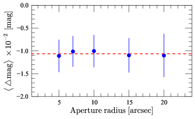
Figure 9: The effect of star-subtraction, a comparison through aperture photometry. The average correction due to star-subtraction effect is $\bigtriangleup\text{m}=-0\!\mbox{$\;\mathrm{.}\!\!^{\textrm{m}}$}0106\pm 0\!\mbox{$\;\mathrm{.}\!\!^{\textrm{m}}$}0003$.

Appendix B Distribution of FP fit parameters

B.1 FP projections

Figure 10 shows different FP projections showing the distribution of the ETGs in Norma (red filled squares) and Coma cluster (in blue open and black filled circles). The blue open circles represent Coma cluster ETGs with $\log\sigma\mathrel{\hbox{$<$}}2$ while the black filled circles represent Coma cluster ETGs with $\log\sigma\geq 2$. The vertical and horizontal dashed red lines represent $\log\sigma=2$, only two galaxies in the Norma sample have $\log\sigma\mathrel{\hbox{$<$}}2$. On the other hand, there are 42 Coma ETGs with $\log\sigma<2$ and 79 ETGs with $\log\sigma\geq 2$.

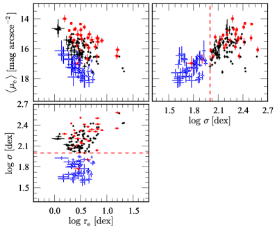
Figure 10: FP projections; the top left panel shows the Kormendy relation. The galaxies in the Norma cluster sample are represented by the red filled squares. The Coma ETGs have been subdivided into two: ETGs with central velocity dispersions less than $100\,\rm{km}\,s^{-1}$ are represented by the blue open circles, while the black filled circles represent Coma ETGs with $\log\sigma\geq 2$.

Using the MIST algorithm, we checked the consistency of the FP fit parameters obtained by regressing along the $\log\sigma$ direction. By re-sampling the Coma cluster (with replacement) 10 000 times, we analysed the distribution of the FP parameters $a$, $b$, and $c$. Figure 11 (left panels) shows the bootstrap results when all the 121 Coma ETGs were used while Fig. 11 (right panels) shows the results for only Coma ETGs brighter than 12​$\;\mathrm{.}\!\!^{\textrm{m}}$5 ($N\!=\!78$, only 9% of these have $\log\sigma\mathrel{\hbox{$<$}}2$). The FP fit parameters in either case, are consistent with each other. The red solid curve is a Gaussian fit to the data. The mean value from the Gaussian fit of each of the FP parameters is indicated at the top part in each panel. The difference between the FP parameter from the original Coma data and that from the fitted distribution through bootstrap is also indicated (as $\Delta a$, $\Delta b$, and $\Delta c$). The blue curve shows the small shift in the Gaussian fit due to this difference, i.e., $\Delta a$, $\Delta b$, and $\Delta c$. The magnitude cut of 12​$\;\mathrm{.}\!\!^{\textrm{m}}$5 was motivated by the fact that it includes majority of Coma ETGs with $\log\sigma\mathrel{\hbox{$>$}}2$, thus making it possible to determine the effect (possible bias) of including ETGs with central velocity dispersions less than 100 km s^-1, on the measured Norma distance. We found the zero-point offset to remain unchanged with and without the magnitude cut, i.e., the small shift $\Delta c$ in Fig. 11 (slightly larger in the left panels than the right panels) is accompanied by small changes in the Fundamental Plane fit parameters $\Delta a$, and $\Delta b$, which in turn affect the FP intercept of the Norma cluster, thereby leaving no significant changes in the zero-point offset.

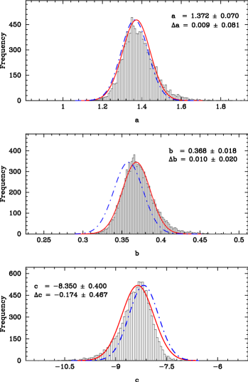
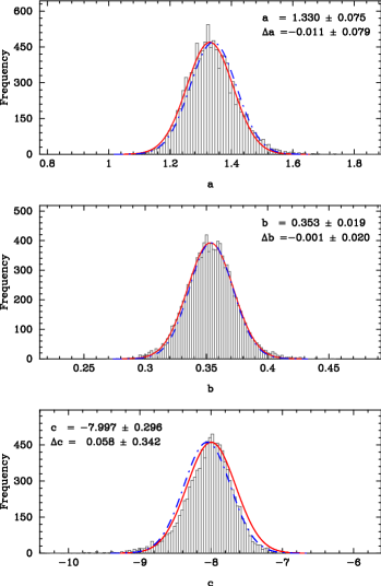
Figure 11: The distribution of the FP fit parameters through bootstrap re-sampling, using the MIST algorithm by minimising along the $\log\,\sigma$- direction. The Coma cluster galaxies were randomly selected, with replacement 10 000 times. The left panels represent results when all the Coma ETGs were used while the right panels represent the bootstrap results for only Coma ETGs brighter than 12$\;\mathrm{.}\!\!^{\textrm{m}}$5. The panels (top to bottom) show the distribution of the FP parameters ($a$, $b$, and $c$). The red curve is the Gaussian fit to the data. The blue curve represents the shift when the Gaussian fit parameters are replaced by FP fit parameters obtained by fitting the original Coma data – the difference is indicated by $\Delta a$, $\Delta b$, and $\Delta c$.

References

- Aaronson et al. (1989) Aaronson M. et al., 1989, ApJ, 338, 654
- Abell et al. (1989) Abell G. O., Corwin Jr. H. G., Olowin R. P., 1989, ApJS, 70, 1
- Aihara et al. (2011) Aihara H. et al., 2011, ApJS, 193, 29
- Allen et al. (1990) Allen D. A., Staveley-Smith L., Meadows V. S., Roche P. F., Norris R. P., 1990, Nature, 343, 45
- Bell et al. (2003) Bell E. F., McIntosh D. H., Katz N., Weinberg M. D., 2003, ApJS, 149, 289
- Bernardi et al. (2002) Bernardi M., Alonso M. V., da Costa L. N., Willmer C. N. A., Wegner G., Pellegrini P. S., Rité C., Maia M. A. G., 2002, AJ, 123, 2159
- Bilicki et al. (2014) Bilicki M., Jarrett T. H., Peacock J. A., Cluver M. E., Steward L., 2014, ApJS, 210, 9
- Boehringer et al. (1996) Boehringer H., Neumann D. M., Schindler S., Kraan-Korteweg R. C., 1996, ApJ, 467, 168
- Bolejko & Hellaby (2008) Bolejko K., Hellaby C., 2008, General Relativity and Gravitation, 40, 1771
- Bonifacio et al. (2000) Bonifacio P., Monai S., Beers T. C., 2000, AJ, 120, 2065
- Branchini et al. (1999) Branchini E. et al., 1999, MNRAS, 308, 1
- Burstein et al. (1990) Burstein D., Faber S. M., Dressler A., 1990, ApJ, 354, 18
- Chincarini & Rood (1979) Chincarini G., Rood H. J., 1979, ApJ, 230, 648
- Colless et al. (2001) Colless M., Saglia R. P., Burstein D., Davies R. L., McMahan R. K., Wegner G., 2001, MNRAS, 321, 277
- Courtois et al. (2012) Courtois H. M., Hoffman Y., Tully R. B., Gottlöber S., 2012, ApJ, 744, 43
- Courtois et al. (2013) Courtois H. M., Pomarède D., Tully R. B., Hoffman Y., Courtois D., 2013, AJ, 146, 69
- da Costa et al. (2000) da Costa L. N., Bernardi M., Alonso M. V., Wegner G., Willmer C. N. A., Pellegrini P. S., Rité C., Maia M. A. G., 2000, AJ, 120, 95
- da Costa et al. (1986) da Costa L. N., Numes M. A., Pellegrini P. S., Willmer C., Chincarini G., Cowan J. J., 1986, AJ, 91, 6
- Djorgovski & Davis (1987) Djorgovski S., Davis M., 1987, ApJ, 313, 59
- Dressler (1980) Dressler A., 1980, ApJS, 42, 565
- Dressler (1988) Dressler A., 1988, ApJ, 329, 519
- Dressler & Faber (1990) Dressler A., Faber S. M., 1990, ApJ, 354, 13
- Dressler et al. (1987) Dressler A., Lynden-Bell D., Burstein D., Davies R. L., Faber S. M., Terlevich R., Wegner G., 1987, ApJ, 313, 42
- Ebeling et al. (2002) Ebeling H., Mullis C. R., Tully R. B., 2002, ApJ, 580, 774
- Ettori et al. (1997) Ettori S., Fabian A. C., White D. A., 1997, MNRAS, 289, 787
- Faber & Jackson (1976) Faber S. M., Jackson R. E., 1976, ApJ, 204, 668
- Harrison (1974) Harrison E. R., 1974, ApJ, 191, L51
- Henning et al. (2000) Henning P. A. et al., 2000, AJ, 119, 2686
- Henning et al. (1999) Henning P. A., Staveley-Smith L., Kraan-Korteweg R. C., Sadler E. M., 1999, Publications of the Astronomical Society of Australia, 16, 35
- Hinshaw et al. (2009) Hinshaw G. et al., 2009, ApJS, 180, 225
- Huang et al. (2013) Huang S., Ho L. C., Peng C. Y., Li Z.-Y., Barth A. J., 2013, ApJ, 766, 47
- Huchra et al. (2012) Huchra J. P. et al., 2012, ApJS, 199, 26
- Hudson (1994) Hudson M. J., 1994, MNRAS, 266, 475
- Hudson et al. (2001) Hudson M. J., Lucey J. R., Smith R. J., Schlegel D. J., Davies R. L., 2001, MNRAS, 327, 265
- Hudson et al. (1997) Hudson M. J., Lucey J. R., Smith R. J., Steel J., 1997, MNRAS, 291, 488
- Hudson et al. (2004) Hudson M. J., Smith R. J., Lucey J. R., Branchini E., 2004, MNRAS, 352, 61
- Hudson et al. (1999) Hudson M. J., Smith R. J., Lucey J. R., Schlegel D. J., Davies R. L., 1999, ApJ, 512, L79
- Jarrett et al. (2000) Jarrett T. H., Chester T., Cutri R., Schneider S., Skrutskie M., Huchra J. P., 2000, AJ, 119, 2498
- Jarrett et al. (2013) Jarrett T. H. et al., 2013, AJ, 145, 6
- Jones et al. (2009) Jones D. H. et al., 2009, MNRAS, 399, 683
- Jorgensen et al. (1995) Jorgensen I., Franx M., Kjaergaard P., 1995, MNRAS, 276, 1341
- Jorgensen et al. (1996) Jorgensen I., Franx M., Kjaergaard P., 1996, MNRAS, 280, 167
- Kocevski & Ebeling (2006) Kocevski D. D., Ebeling H., 2006, ApJ, 645, 1043
- Kraan-Korteweg et al. (2000) Kraan-Korteweg R. C., Henning P. A., Andernach H., eds, 2000, Mapping the Hidden Universe: The Universe behind the Milky Way - The Universe in HI Astronomical Society of the Pacific Conference Series Vol. 218
- Kraan-Korteweg et al. (2011) Kraan-Korteweg R. C., Riad I. F., Woudt P. A., Nagayama T., Wakamatsu K., 2011, ArXiv e-prints
- Kraan-Korteweg et al. (1996) Kraan-Korteweg R. C., Woudt P. A., Cayatte V., Fairall A. P., Balkowski C., Henning P. A., 1996, Nature, 379, 519
- La Barbera et al. (2000) La Barbera F., Busarello G., Capaccioli M., 2000, A&A, 362, 851
- La Barbera et al. (2010) La Barbera F., de Carvalho R. R., de La Rosa I. G., Lopes P. A. A., 2010, MNRAS, 408, 1335
- Lagattuta et al. (2013) Lagattuta D. J., Mould J. R., Staveley-Smith L., Hong T., Springob C. M., Masters K. L., Koribalski B. S., Jones D. H., 2013, ApJ, 771, 88
- Lavaux et al. (2010) Lavaux G., Tully R. B., Mohayaee R., Colombi S., 2010, ApJ, 709, 483
- Lewis et al. (2002) Lewis I. J. et al., 2002, MNRAS, 333, 279
- Lilje et al. (1986) Lilje P. B., Yahil A., Jones B. J. T., 1986, ApJ, 307, 91
- Lucey et al. (2005) Lucey J., Radburn-Smith D., Hudson M., 2005, in A. P. Fairall & P. A. Woudt ed., Astronomical Society of the Pacific Conference Series Vol. 329, Nearby Large-Scale Structures and the Zone of Avoidance. pp 21–+
- Lucey (1986) Lucey J. R., 1986, MNRAS, 222, 417
- Lucey & Carter (1988) Lucey J. R., Carter D., 1988, MNRAS, 235, 1177
- Lynden-Bell et al. (1988) Lynden-Bell D., Faber S. M., Burstein D., Davies R. L., Dressler A., Terlevich R. J., Wegner G., 1988, ApJ, 326, 19
- Lynden-Bell et al. (1989) Lynden-Bell D., Lahav O., Burstein D., 1989, MNRAS, 241, 325
- Magoulas et al. (2012) Magoulas C. et al., 2012, MNRAS, 427, 245
- Marinoni et al. (1998) Marinoni C., Monaco P., Giuricin G., Costantini B., 1998, ApJ, 505, 484
- Mathewson et al. (1992) Mathewson D. S., Ford V. L., Buchhorn M., 1992, ApJS, 81, 413
- Mould et al. (2000) Mould J. R. et al., 2000, ApJ, 529, 786
- Nagayama et al. (2006) Nagayama T. et al., 2006, MNRAS, 368, 534
- Oort (1983) Oort J. H., 1983, ARA&A, 21, 373
- Pahre (1999) Pahre M. A., 1999, ApJS, 124, 127
- Peng et al. (2010) Peng C. Y., Ho L. C., Impey C. D., Rix H., 2010, AJ, 139, 2097
- Proust et al. (2006) Proust D. et al., 2006, A&A, 447, 133
- Radburn-Smith et al. (2006) Radburn-Smith D. J., Lucey J. R., Woudt P. A., Kraan-Korteweg R. C., Watson F. G., 2006, MNRAS, 369, 1131
- Raychaudhury (1989) Raychaudhury S., 1989, Nature, 342, 251
- Rowan-Robinson et al. (1990) Rowan-Robinson M. et al., 1990, MNRAS, 247, 1
- Rubin et al. (1976) Rubin V. C., Roberts M. S., Graham J. A., Ford Jr. W. K., Thonnard N., 1976, AJ, 81, 687
- Said (2013) Said K., 2013, Master’s thesis, Univ. Cape Town
- Sandage (1975) Sandage A., 1975, ApJ, 202, 563
- Sargent et al. (1977) Sargent W. L. W., Schechter P. L., Boksenberg A., Shortridge K., 1977, ApJ, 212, 326
- Saunders et al. (2000) Saunders W. et al., 2000, MNRAS, 317, 55
- Scaramella et al. (1989) Scaramella R., Baiesi-Pillastrini G., Chincarini G., Vettolani G., Zamorani G., 1989, Nature, 338, 562
- Schlafly & Finkbeiner (2011) Schlafly E. F., Finkbeiner D. P., 2011, ApJ, 737, 103
- Schlegel et al. (1998) Schlegel D. J., Finkbeiner D. P., Davis M., 1998, ApJ, 500, 525
- Schröder et al. (2009) Schröder A. C., Kraan-Korteweg R. C., Henning P. A., 2009, A&A, 505, 1049
- Schröder et al. (2007) Schröder A. C., Mamon G. A., Kraan-Korteweg R. C., Woudt P. A., 2007, A&A, 466, 481
- Sersic (1968) Sersic J. L., 1968, Atlas de galaxias australes
- Shapley (1930) Shapley H., 1930, Harvard College Observatory Bulletin, 874, 9
- Shaya (1984) Shaya E. J., 1984, ApJ, 280, 470
- Shaya & Tully (2013) Shaya E. J., Tully R. B., 2013, MNRAS, 436, 2096
- Skelton et al. (2009) Skelton R. E., Woudt P. A., Kraan-Korteweg R. C., 2009, MNRAS, 396, 2367
- Skrutskie et al. (2006) Skrutskie M. F. et al., 2006, AJ, 131, 1163
- Sorce et al. (2012) Sorce J. G., Courtois H. M., Tully R. B., 2012, AJ, 144, 133
- Springob et al. (2007) Springob C. M., Masters K. L., Haynes M. P., Giovanelli R., Marinoni C., 2007, ApJS, 172, 599
- Stetson (1987) Stetson P. B., 1987, PASP, 99, 191
- Strauss & Davis (1988) Strauss M. A., Davis M., 1988, in Audouze J., Pelletan M.-C., Szalay A., Zel’dovich Y. B., Peebles P. J. E., eds, IAU Symposium Vol. 130, Large Scale Structures of the Universe. p. 191
- Strauss & Willick (1995) Strauss M. A., Willick J. A., 1995, Phys. Rep., 261, 271
- Tammann & Sandage (1985) Tammann G. A., Sandage A., 1985, ApJ, 294, 81
- Tonry et al. (2000) Tonry J. L., Blakeslee J. P., Ajhar E. A., Dressler A., 2000, ApJ, 530, 625
- Tully et al. (2013) Tully R. B. et al., 2013, AJ, 146, 86
- Tully et al. (2009) Tully R. B., Rizzi L., Shaya E. J., Courtois H. M., Makarov D. I., Jacobs B. A., 2009, AJ, 138, 323
- Vollmer et al. (2001) Vollmer B., Cayatte V., van Driel W., Henning P. A., Kraan-Korteweg R. C., Balkowski C., Woudt P. A., Duschl W. J., 2001, A&A, 369, 432
- Woudt & Kraan-Korteweg (2001) Woudt P. A., Kraan-Korteweg R. C., 2001, A&A, 380, 441
- Woudt et al. (2008) Woudt P. A., Kraan-Korteweg R. C., Lucey J., Fairall A. P., Moore S. A. W., 2008, MNRAS, 383, 445
- Yasuda et al. (2007) Yasuda N., Fukugita M., Schneider D. P., 2007, AJ, 134, 698