Iterative construction of eigenfunctions of the monodromy matrix for $SL(2,\mathbb{C})$ magnet.

Abstract

Eigenfunctions of the matrix elements of the monodromy matrix provide a convenient basis for studies of spin chain models. We present an iterative method for constructing the eigenfunctions in the case of the $SL(2,\mathbb{C})$ spin chains. We derived an explicit integral representation for the eigenfunctions and calculated the corresponding scalar products (Sklyanin’s measure).

1 Introduction

The quantum inverse scattering method is a powerful tool for constructing and solving integrable models. The fundamental object in this approach is the so-called $\mathcal{R}-$matrix – a linear operator which depends on a complex parameter (spectral parameter) and satisfies a certain nonlinear relation known as the Yang - Baxter equation (YBE). Each solution of this equation gives rise to a family of commuting operators. In many cases a commutative family includes an operator which can be identified with a Hamiltonian of some physical system. The most famous example of an such integrable system is the $\mathrm{XXX}_{1/2}$-spin chain – the celebrated Heisenberg spin $1/2$ magnet solved by H. Bethe in 1931 [1]. The general algebraic framework was developed much later and became known as Quantum Inverse Scattering Method (QISM). For a review and references see Refs. [2, 3, 4, 5, 6, 7].

Integrable models with a finite dimensional Hilbert space such as spin magnets of different types, found many applications in statistical and solid state physics [2]. Quite unexpectedly spin magnets arise also in the studies of high-energy scattering amplitudes in quantum field theories, namely in the gauge field theories. Most of them can be solved with the help of the Algebraic Bethe Ansatz(ABA) [3, 4, 5, 6, 7]. In this approach eigenstates of the model are constructed as excitations of certain type over the special (preudovacuum) state belonging to the Hilbert space of the system. However, there are integrable models, e.g. the Toda chain [8, 9, 10, 11] and the quantum KdV model [12, 13], which can not be solved within the ABA. Such models have an infinite - dimensional Hilbert space and the pseudovacuum state does not belong to it. Nevertheless they can be solved by the methods of Baxter $\mathcal{Q}-$operators [14] and Separation of Variables (SoV) [15].

In the present work we consider another model of this type – the so-called noncompact $SL(2,\mathbb{C})$ spin magnet. Interest to such models stems from the studies of Regge behaviour of hadron scattering amplitudes, for a review see Ref. [16]. It turns out that the Hamiltonian which governs the scale dependence of the scattering amplitudes in high - energy limit is integrable and can be identified with the Hamiltonian of a spin magnet [17, 18, 19]. This model was solved in Refs. [20, 21, 22, 23] with the help of Baxter $\mathcal{Q}-$operators and SoV methods. Recently it was argued that the behaviour of scattering amplitudes in the multi-Regge kinematics in $\mathcal{N}=4$ SUSY is governed by the Hamiltonian of the noncompact open spin chain [24, 25]. The Hamiltonian of the model commutes with the diagonal entry of the monodromy matrix, $D(u)$. In both cases, in order to diagonalize the Hamiltonian one has first to construct eigenfunctions for entries of the monodromy matrix ($B$ or $D$). Let us also mention that the problem of diagonalization of the operator $D$ for finite dimensional representations of the $SL(2)$ group was addressed in Refs. [26, 27].

In this work we provide a regular recurrence procedure for constructing eigenfunctions for all entries of the monodromy matrix. Our approach relies heavily on the representation of the $sl(2)-$invariant $\mathcal{R}-$matrix in the factorized form [28, 29]. The operators which factorize the $\mathcal{R}-$matrix play a prominent role in our construction. Using them one can construct operators that intertwine the entries of the monodromy matrix for the chains of different length ($B_{N}(u)\Lambda_{N}\sim\Lambda_{N}B_{N-1}(u)$, an so on). It immediately leads to a recurrence construction. We derive an integral representation for the eigenfunctions and calculate their scalar products (Sklyanin’s measure).

It was shown by Sklyanin [7] that the eigenvalue equations for the transfer matrix for the rank one chain models become separated in the basis provided by the eigenfunctions of the operator $B_{N}(u)$. At present time the SoV representation is known for a variety of models. Among them are the Toda chain [11, 30, 31, 32], different types of $XXX$ [22, 33, 34, 35] and $XXZ$ spin chains [36, 37, 38, 39].

The paper is organized as follows: In Sect. 2 we describe the model and some basic elements of the QISM method. In Sect.3 we develop an iterative procedure for constructing the eigenfunctions of the elements of the monodromy matrix. In Sect. 4 we calculate scalar products of the eigenfunctions and determine the Sklyanin measure. The method of constructing the Baxter operators is described in Sect. 5. The Hamiltonians for $D-$system are discussed in Sect. 6. Concluding remarks are presented in Sect. 7. Several Appendices contain technical details.

2 Preliminaries

The quantum $SL(2,\mathbb{C})$ spin magnet is a straightforward generalization of the standard $\mathrm{XXX}_{s}$ spin chain. In both models the dynamical variables are the spin operators, $\vec{S}_{k}$, $k=1,\ldots,N$, where $N$ is the length of the chain. In the $\mathrm{XXX}_{s}$ model the spin operators belong to a finite dimensional representation of the $SU(2)$ group so that the Hilbert space of the model is finite dimensional. In the case of the $SL(2,\mathbb{C})$ spin magnet the spin generators belong to a unitary continuous principal series representation of the $SL(2,\mathbb{C})$ group and the corresponding Hilbert space is infinite dimensional.

The unitary principal series representation of the $SL(2,\mathbb{C})$ group, $T^{(s,\bar{s})}$, is determined by two complex numbers (spins), $s$ and $\bar{s}$, such that $s-\bar{s}$ is a half-integer and $s+\bar{s}^{*}=1$ [40]. It acts on the space $L_{2}(\mathbb{C})$ and the group transformations take the form

$$[T^{(s,\bar{s})}(g^{-1})f](z,\bar{z})=(cz+d)^{-2s}(\bar{c}\bar{z}+\bar{d})^{-2\bar{s}}\,f\left(\frac{az+b}{cz+d},\frac{\bar{a}\bar{z}+\bar{b}}{\bar{c}\bar{z}+\bar{d}}\right)\,.$$ (1)

Here $g$ is a complex unimodular matrix, $g=\left(\begin{array}[]{cc}a&b\\ c&d\end{array}\right)$, $ab-cd=1$, and $f\in L_{2}(\mathbb{C})$. For the unitary representations the spins $s$, $\bar{s}$ can be parameterized as follows

$$s=\frac{1+n_{s}}{2}+i\nu_{s},\qquad\qquad\bar{s}=\frac{1-n_{s}}{2}+i\nu_{s},$$ (2)

where $n_{s}$ is half-integer and $\nu_{s}$ is real. The operators (1) are unitary with respect to the standard scalar product

$$(f,\psi)=\int d^{2}z\bar{f}(z)\psi(z),\qquad\qquad(T^{(s,\bar{s})}(g)f,T^{(s,\bar{s})}(g)\psi)=(f,\psi).$$ (3)

The generators of infinitesimal transformations (spin operators) take the form

$$S_{-}=-\partial_{z},\qquad S_{0}=z\partial_{z}+s,\qquad S_{+}=z^{2}\partial_{z}+2sz\,,$$

$$\bar{S}_{-}=-\partial_{\bar{z}},\qquad\bar{S}_{0}={\bar{z}}\partial_{\bar{z}}+\bar{s},\qquad\bar{S}_{+}=\bar{z}^{2}\partial_{\bar{z}}+2\bar{s}\bar{z}\,$$ (4)

and satisfy the standard $sl(2)$ commutation relations

$$[S_{+},S_{-}]=2S_{0},\qquad[S_{0},S_{\pm}]=\pm S_{\pm},$$

$${}[\bar{S}_{+},\bar{S}_{-}]=2\bar{S}_{0},\qquad[\bar{S}_{0},\bar{S}_{\pm}]=\pm\bar{S}_{\pm}.$$ (5)

The holomorphic ($S_{\alpha}$) and anti-holomorphic ($\bar{S}_{\alpha}$) generators commute. For the unitary representations the holomorphic and anti-holomorphic generators are adjoint to each other, $S_{\alpha}^{\dagger}=-\bar{S}_{\alpha}$.

Summarising: The quantum $SL(2,\mathbb{C})$ spin magnet is a one-dimensional lattice model. The Hilbert space of the model is given by the direct product of the $L_{2}(\mathbb{C})$ spaces,

$$\mathbb{H}_{N}=\mathbb{V}_{1}\otimes\mathbb{V}_{2}\otimes\ldots\otimes\mathbb{V}_{N},\qquad\mathbb{V}_{k}=L_{2}(\mathbb{C})\,,\qquad k=1,\ldots,N.$$ (6)

The dynamical variables are given by two sets of spin operators  – holomorphic ( $S^{(k)}_{\pm,0}$ ) and anti-holomorphic ( $\bar{S}^{(k)}_{\pm,0}$ ), $k=1,\ldots,N$. In what follows we will consider only homogeneous chains, $s_{k}=s$, $\bar{s}_{k}=\bar{s}$, for all $k$.

2.1 $L$ operators and monodromy matrices

$L-$operators play a fundamental role in the theory of integrable systems. In the case of spin magnets they are defined as follows

$$L(u)=u+i\left(\begin{array}[]{cc}S_{0}&S_{-}\\ S_{+}&-S_{0}\end{array}\right)\,,\qquad\bar{L}(\bar{u})=\bar{u}+i\left(\begin{array}[]{cc}\bar{S}_{0}&\bar{S}_{-}\\ \bar{S}_{+}&-\bar{S}_{0}\end{array}\right)\,.$$ (7)

Here $u,\bar{u}$ are two complex numbers (spectral parameters). Note that $L(u)\,\big{(}\bar{L}(\bar{u})\big{)}$ acts on a tensor product of $L_{2}(\mathbb{C})$ and a two dimensional complex vector space (auxiliary space), $\mathbb{V}_{0}\equiv\mathbb{C}^{2}$. The operators $L(u)$ and $L^{\prime}(v)$ acting on $L_{2}(\mathbb{C})\otimes\mathbb{V}_{0}$ and $L_{2}(\mathbb{C})\otimes\mathbb{V}_{0^{\prime}}$, respectively, satisfy the fundamental commutation relation (FCR)

$$\mathcal{R}_{00^{\prime}}(u-v)L(u)L^{\prime}(v) = L^{\prime}(v)L(u)\mathcal{R}_{00^{\prime}}(u-v)\,,$$

$$\mathcal{R}_{00^{\prime}}(\bar{u}-\bar{v})\bar{L}(\bar{u})\bar{L}^{\prime}(\bar{v}) = \bar{L}^{\prime}(\bar{v})\bar{L}(\bar{u})\mathcal{R}_{00^{\prime}}(\bar{u}-\bar{v})\,,$$ (8)

The operator $\mathcal{R}_{00^{\prime}}(u)$ ($\mathcal{R}-$matrix) acts on the tensor product of two auxiliary spaces, $\mathbb{V}_{0}\otimes\mathbb{V}_{0^{\prime}}=\mathbb{C}^{2}\otimes\mathbb{C}^{2}$, and has the form $\mathcal{R}_{00^{\prime}}(u)=u+iP_{00^{\prime}}$ where $P_{00^{\prime}}$ is the permutation operator on $\mathbb{V}_{0}\otimes\mathbb{V}_{0^{\prime}}$. The monodromy matrix is defined as a product of $L$ operators acting on the same auxiliary but different quantum spaces

$$T(u)=L_{1}(u)L_{2}(u)\ldots L_{N}(u)\,,\qquad\bar{T}(\bar{u})=\bar{L}_{1}(\bar{u})\bar{L}_{2}(\bar{u})\ldots\bar{L}_{N}(\bar{u})\,.$$ (9)

The $L-$operator with subscript $k$ acts nontrivially on the $k-$th space in the ternsor product (6). The monodromy matrix $T_{N}(u)$ ( $\bar{T}_{N}(\bar{u})$ ) is a two by two matrix in the auxiliary space with entries that are operators on the quantum space $\mathbb{H}_{N}$

$$T(u)=\left(\begin{array}[]{cc}A_{N}(u)&B_{N}(u)\\ C_{N}(u)&D_{N}(u)\end{array}\right)\,,\qquad\bar{T}(\bar{u})=\left(\begin{array}[]{cc}\bar{A}_{N}(\bar{u})&\bar{B}_{N}(\bar{u})\\ \bar{C}_{N}(\bar{u})&\bar{D}_{N}(\bar{u})\end{array}\right)\,.$$ (10)

Monodromy matrices satisfy the same commutation relation as $L-$operators, Eq. (2.1)

$$\mathcal{R}_{00^{\prime}}(u-v)T_{N}(u)T^{\prime}_{N}(v) = T^{\prime}_{N}(v)T_{N}(u)\mathcal{R}_{00^{\prime}}(u-v)\,,$$

$$\mathcal{R}_{00^{\prime}}(\bar{u}-\bar{v})\bar{T}_{N}(\bar{u})\bar{T}^{\prime}_{N}(\bar{v}) = \bar{T}^{\prime}_{N}(\bar{v})\bar{T}_{N}(\bar{u})\mathcal{R}_{00^{\prime}}(\bar{u}-\bar{v})\,.$$ (11)

These equations result in certain algebraic relations for the entries of the monodromy matrices. In particular, they imply that all operators commute with themselves for different values of the spectral parameter

$$[A_{N}(u),A_{N}(v)]=0,\qquad[B_{N}(u),B_{N}(v)]=0,$$

$${}[C_{N}(u),C_{N}(v)]=0,\qquad[D_{N}(u),D_{N}(v)]=0$$ (12)

and similar for all others. By construction the operators $A_{N}(u),D_{N}(u)$ are polynomials of degree $N$ in $u$, while the operators $B_{N}(u),C_{N}(u)$ are polynomials of a degree $N-1$,

$$A_{N}(u)=u^{N}+iu^{N-1}S_{0}+\sum_{k=2}^{N}u^{N-k}a_{k}\,,\qquad B_{N}(u)=iS_{-}u^{N-1}+\sum_{k=2}^{N}u^{N-k}b_{k}\,,$$

$$D_{N}(u)=u^{N}-iu^{N-1}S_{0}+\sum_{k=2}^{N}u^{N-k}d_{k}\,,\qquad C_{N}(u)=iS_{+}u^{N-1}+\sum_{k=2}^{N}u^{N-k}c_{k}\,,$$ (13)

where $S_{\alpha}=\sum_{k=1}^{N}S_{\alpha}^{(k)}$ are the operators of total spin. The construction for anti-holomorphic sector is essentially the same and we will omit the corresponding similar expressions as a rule. It follows from (2.1), (2.1) that $[S_{0},a_{k}]=[a_{i},a_{k}]=0$ for all $i,k$ and similar for $b_{k},c_{k},d_{k}$ operators. Taking into account that $A_{N}(u)^{\dagger}=\bar{A}_{N}(u^{*})$ one concludes that the operators

$$i(S_{0}+\bar{S}_{0}),\qquad S_{0}-\bar{S}_{0},\qquad a^{+}_{k}=\frac{1}{2}(a_{k}+\bar{a}_{k}),\qquad a^{-}_{k}=\frac{i}{2}(a_{k}-\bar{a}_{k})\,,$$ (14)

form a set of commuting self-adjoint operators,

$$\mathcal{A}_{N}=\Big{\{}i(S_{0}+\bar{S}_{0}),\,S_{0}-\bar{S}_{0},\,a^{+}_{k},\,a^{-}_{k},\,\quad k=2,\ldots N\Big{\}}$$ (15)

and hence can be diagonalized simultaneously. We want to stress here that self-adjointness which does not play any essential role in an analysis of finite-dimensional models is very important in the case under consideration .

The operators $A_{N}(u),B_{N}(u),\ldots$ are differential operators of $N-$th order in the variables $z_{1},\ldots,z_{N}$. Let $\Psi_{A}(\boldsymbol{z})=\Psi_{A}(z_{1},\bar{z}_{1}\ldots,z_{N},\bar{z}_{N})$ be an eigenfunction of the operators $A_{N}(u),\bar{A}_{N}(\bar{u})$. By virtue of Eq. (2.1) the corresponding eigenvalues are polynomials of degree $N$ in $u$, $\bar{u}$, respectively. The eigenfunctions can be labelled by zeroes of these polynomials, i.e.

$$A_{N}(u)\,\Psi_{A}({\boldsymbol{x}}|\boldsymbol{z}) = (u-x_{1})\ldots(u-x_{N})\,\Psi_{A}({\boldsymbol{x}}|\boldsymbol{z})\,,$$

$$\bar{A}_{N}(\bar{u})\,\Psi_{A}({\boldsymbol{x}}|\boldsymbol{z}) = (\bar{u}-\bar{x}_{1})\ldots(\bar{u}-\bar{x}_{N})\,\Psi_{A}({\boldsymbol{x}}|\boldsymbol{z})\,,$$ (16)

where

$${\boldsymbol{x}}=\{\boldsymbol{x}_{1},\ldots,\boldsymbol{x}_{N}\}, \boldsymbol{x}_{k}=(x_{k},\bar{x}_{k})$$

$$\boldsymbol{z}=\{\boldsymbol{z}_{1},\ldots,\boldsymbol{z}_{N}\}, \boldsymbol{z}_{k}=(z_{k},\bar{z}_{k}).$$ (17)

Note that a behaviour of the eigenfunction under the scale transformations, $z\to\lambda z$, is controlled by the sum $i\sum_{k}x_{k}$ (which is the eigenvalue of the operator $S_{0}$)

$$\Psi_{A}({\boldsymbol{x}}|\lambda\boldsymbol{z})=\lambda^{-Ns+i\sum_{k}x_{k}}\bar{\lambda}^{-N\bar{s}+i\sum_{k}\bar{x}_{k}}\Psi_{A}({\boldsymbol{x}}|\boldsymbol{z})\,.$$ (18)

In full analogy with the previous case the operators $B_{N},\bar{B}_{N}$ give rise to another set of the commuting operators,

$$\mathcal{B}_{N}=\Big{\{}i(S_{-}+\bar{S}_{-}),\ S_{-}-\bar{S}_{-},\ b^{+}_{k}=\frac{1}{2}(b_{k}+\bar{b}_{k}),\ b^{-}_{k}=\frac{i}{2}(b_{k}-\bar{b}_{k}),\ k=2,\ldots N-1\Big{\}}.$$ (19)

The eigenfunctions can be parameterized by the momenta $p,\bar{p}$, which are the eigenvalues of the $S_{-},\bar{S}_{-}$ operators and the roots of $x_{k},\bar{x}_{k}$, $k=1,\ldots,N-1$ of the corresponding eigenvalues

$$B_{N}(u)\,\Psi_{B}({\boldsymbol{x}}|\boldsymbol{z}) = p(u-x_{1})\ldots(u-x_{N-1})\,\Psi_{B}({\boldsymbol{x}}|\boldsymbol{z})\,,$$

$$\bar{B}_{N}(\bar{u})\,\Psi_{B}({\boldsymbol{x}}|\boldsymbol{z}) = \bar{p}(\bar{u}-\bar{x}_{1})\ldots(\bar{u}-\bar{x}_{N-1})\,\Psi_{B}({\boldsymbol{x}}|\boldsymbol{z})\,.$$ (20)

In order to keep the same notations for the $A$ and $B$ cases, we have put $x_{N}=p,\bar{x}_{N}=\bar{p}$, i.e.

$${\boldsymbol{x}}=\{\boldsymbol{x}_{1},\ldots,\boldsymbol{x}_{N-1},\boldsymbol{x}_{N}=(p,\bar{p})\}\,.$$ (21)

It will be shown below that eigenfunctions of the operators $D_{N}$ and $C_{N}$ are related to those of $A_{N}$ and $B_{N}$ by an inversion transformation. In sect. 3 we present an iterative procedure for constructing the eigenfunctions. It relies on the properties of operators that factorize the general $\mathcal{R}-$matrix, which are discussed in the next section.

2.2 $\mathcal{R}$-matrix and factorizing operators

General $\mathcal{R}-$matrix is defined as a solution of the $RLL-$relation [41]

$$\mathcal{R}_{\boldsymbol{s}_{1}\boldsymbol{s}_{2}}(u-v,\bar{u}-\bar{v})L_{s_{1}}(u)L_{s_{2}}(v) = L_{s_{2}}(v)L_{s_{1}}(u)\mathcal{R}_{\boldsymbol{s}_{1}\boldsymbol{s}_{2}}(u-v,\bar{u}-\bar{v})\,,$$

$$\mathcal{R}_{\boldsymbol{s}_{1}\boldsymbol{s}_{2}}(u-v,\bar{u}-\bar{v})\bar{L}_{\bar{s}_{1}}(\bar{u})\bar{L}_{\bar{s}_{2}}(\bar{v}) = \bar{L}_{\bar{s}_{2}}(\bar{v})\bar{L}_{\bar{s}_{1}}(u)\mathcal{R}_{\boldsymbol{s}_{1}\boldsymbol{s}_{2}}(u-v,\bar{u}-\bar{v})\,.$$ (22)

Here $L-$operators act in the same auxiliary space but in different quantum spaces and the operator $\mathcal{R}_{\boldsymbol{s}_{1}\boldsymbol{s}_{2}}$ maps $L_{2}(\mathbb{C})\otimes L_{2}(\mathbb{C})\mapsto L_{2}(\mathbb{C})\otimes L_{2}(\mathbb{C})$. The labels $\boldsymbol{s}_{k}=(s_{k},\bar{s}_{k})$ indicate the representation of the $SL(2,\mathbb{C})$ group in the first and second quantum spaces. The operator $\mathcal{R}_{\boldsymbol{s}_{1}\boldsymbol{s}_{2}}$ satisfying Eqs. (2.2) was constructed as an integral operator in Ref. [22]. Later it has been suggested to look for the solutions of Eq. (2.2) in a factorized form [28]. Below we briefly describe the corresponding construction. First we note that the $L-$operator depends on two parameters: the spectral parameter $\boldsymbol{u}$ and the spin $\boldsymbol{s}$. It is convenient to define two linear combinations 

$$u_{1}=u-i(1-s)\,,\qquad u_{2}=u-is.$$ (23)

Thus $L_{s_{1}}(u)=L(u_{1},u_{2})$ and $L_{s_{2}}(v)=L(v_{1},v_{2})$. Factoring out the permutation operator from $\mathcal{R}-$matrix, $\mathcal{R}_{\boldsymbol{s}_{1}\boldsymbol{s}_{2}}=P_{12}\widehat{\mathcal{R}}_{12}$, one gets the following equation on $\widehat{\mathcal{R}}_{12}$

$$\widehat{\mathcal{R}}_{12}\,L_{1}(u_{1},u_{2})L_{2}(v_{1},v_{2})=L_{1}(v_{1},v_{2})L_{2}(u_{1},u_{2})\,\widehat{\mathcal{R}}_{12}\,.$$ (24)

The operator $L_{1}(L_{2})$ acts on the first (second) space in the tensor product, $L_{2}(\mathbb{C})\otimes L_{2}(\mathbb{C})$ (i.e. $L_{1}$ and $L_{2}$ are the differential operators in $z_{1}$ and $z_{2}$, respectively.) Thus the operator $\widehat{\mathcal{R}}_{12}$ interchanges the parameters $(u_{1},u_{2})\leftrightarrow(v_{1},v_{2})$ in the product of two $L$ operators. It is natural to break this permutation of the parameters into two operations and construct the operators which interchange the parameters $u_{1}\leftrightarrow v_{1}$ and $u_{2}\leftrightarrow v_{2}$ in the product of $L-$operators separately

$${\mathcal{R}^{(1)}_{12}}\,L_{1}(u_{1},u_{2})L_{2}(v_{1},v_{2}) = L_{1}(v_{1},u_{2})L_{2}(u_{1},v_{2})\,{\mathcal{R}^{(1)}_{12}}\,,$$

$${\mathcal{R}^{(2)}_{12}}\,L_{1}(u_{1},u_{2})L_{2}(v_{1},v_{2}) = L_{1}(u_{1},v_{2})L_{2}(v_{1},u_{2})\,{\mathcal{R}^{(2)}_{12}}\,.$$ (25)

It turns out that the operators $\mathcal{R}^{(a)}_{12}$ depend only on the specific combinations of the spectral parameters 

$$\mathcal{R}^{(1)}_{12}=\mathcal{R}^{(1)}_{12}(u_{1}-v_{1},u_{1}-v_{2}),\qquad\mathcal{R}^{(2)}_{12}=\mathcal{R}^{(2)}_{12}(u_{1}-v_{2},u_{2}-v_{2})$$ (26)

and have a remarkably simple form [28, 29]

$$[\mathcal{R}^{(1)}_{12}(u_{1}-v_{1},u_{1}-v_{2})\Phi](z_{1},z_{2}) = \int d^{2}w_{2}\,\frac{[z_{2}-z_{1}]^{i(v_{1}-v_{2})}}{[z_{2}-w_{2}]^{1-i(u_{1}-v_{1})}[z_{1}-w_{2}]^{i(u_{1}-v_{2})}}\,\Phi(z_{1},w_{2})\,,$$

$$[\mathcal{R}^{(2)}_{12}(u_{1}-v_{2},u_{2}-v_{2})\Phi](z_{1},z_{2}) = \int d^{2}w_{1}\,\frac{[z_{1}-z_{2}]^{i(u_{1}-u_{2})}}{[w_{1}-z_{1}]^{1-i(u_{2}-v_{2})}[w_{1}-z_{2}]^{i(u_{1}-v_{2})}}\,\Phi(w_{1},z_{2})\,,$$ (27)

where $[a]^{\alpha}\equiv a^{\alpha}\,\bar{a}^{\bar{\alpha}}$ which is a single valued function in the complex plane provided that $\alpha-\bar{\alpha}\in\mathbb{Z}$. The requirement of single-valuedness of the kernels results in quantization of the spectral parameters, $u,\bar{u}$, $u-\bar{u}\in\mathbb{Z}$ [22], which were so far considered as independent variables.

Finally, the $\mathcal{R}-$matrix satisfying $RLL-$relation (2.2) is constructed as follows

$$\mathcal{R}_{\boldsymbol{s}_{1}\boldsymbol{s}_{2}}(u-v,\bar{u}-\bar{v})=P_{12}\mathcal{R}^{(1)}_{12}(u_{1}-v_{1},u_{1}-u_{2})\mathcal{R}^{(2)}_{12}(u_{1}-v_{2},u_{2}-v_{2})\,.$$ (28)

For a more detailed discussion of properties of factorizing operators see Ref. [42, 29].

3 Iterative construction of eigenfunctions

We present in this section a recurrence procedure of construction the eigenfunctions of the operators $A_{N}(u)$, $B_{N}(u)$. (For simplicity we consider the homogeneous spin chain $s_{k}=s,\bar{s}_{k}=\bar{s}$ though the construction are easily generalized for general case.)

Let us consider a modified monodromy matrix

$${T}_{N}(u,v)=L_{1}(u_{1},v)L_{2}(u_{1},u_{2})\ldots L_{N}(u_{1},u_{2})\,.$$ (29)

Here all $L-$operators except the first one has a standard form ($L_{k}(u)=L_{k}(u_{1},u_{2})$) while in the first one we replace the parameter $u_{2}=u-is\to v$. Taking into account that the first row of the $L-$operators does not change under this substitution (see Eqs. (7),(23))

$$L_{1}(u_{1},v_{1})=\left(\begin{array}[]{cc}u+iS^{(1)}_{0}&S_{-}^{(1)}\\ \star&\star\end{array}\right)$$ (30)

one immediately gets that such a modification leaves the elements in the first row of the monodromy matrix intact,

$${T}_{N}(u,v)=\left(\begin{array}[]{cc}A_{N}(u)&B_{N}(u)\\ \star&\star\end{array}\right)\,.$$ (31)

Let us consider the commutation relation of the monodromy matrix ${T}_{N}(u,v)$ with an operator $\boldsymbol{\Lambda}_{N}(u,v)$ defined by 

$$\boldsymbol{\Lambda}_{N}(u,v)=\mathcal{R}^{(2)}_{12}(u_{1}-v,u_{2}-v)\mathcal{R}^{(2)}_{23}(u_{1}-v,u_{2}-v)\ldots\mathcal{R}^{(2)}_{N-1,N}(u_{1}-v,u_{2}-v)\,.$$ (32)

Taking into account the relations (2.2) one obtains

$${T}_{N}(u,v)\,\boldsymbol{\Lambda}_{N}(u,v)=\boldsymbol{\Lambda}_{N}(u,v)\,{T}_{N-1}(u)\,L_{N}(u_{1},v)\,,$$ (33)

where ${T}_{N-1}(u)=L_{1}(u)\ldots L_{N-1}(u)$. Comparing the matrix elements in the first row of the l.h.s and r.h.s of Eq. (33) one gets

$$A_{N}(u)\boldsymbol{\Lambda}_{N}(u,v) = \boldsymbol{\Lambda}_{N}(u,v)\Big{(}A_{N-1}(u)(u+is+iz_{N}\partial_{z_{N}})+B_{N-1}(u)z_{N}(iz_{N}\partial_{z_{N}}+v-u_{1}+i)\Big{)}\,,$$

$$B_{N}(u)\boldsymbol{\Lambda}_{N}(u,v) = \boldsymbol{\Lambda}_{N}(u,v)\Big{(}B_{N-1}(u)(v-iz_{N}\partial_{z_{N}})-A_{N-1}(u)\partial_{z_{N}}\Big{)}\,.$$ (34)

3.1 $B-$system

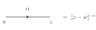
Figure 1: The diagrammatic representation of the propagator.

Let us apply the operators on both sides of the second of Eqs. (3) to the function $\Psi(z_{1},\ldots,z_{N-1})$ which does not depend on the variable $z_{N}$. In this case the second term on the r.h.s. ($A_{N-1}(u)\partial_{z_{N}}$) vanishes and the equation takes the form

$$B_{N}(u)\,\boldsymbol{\Lambda}_{N}(u,v)\,\Psi(z_{1},\ldots,z_{N-1})=v\,\boldsymbol{\Lambda}_{N}(u,v)\,B_{N-1}(u)\,\Psi(z_{1},\ldots,z_{N-1})\,,$$ (35)

so that the operator $\boldsymbol{\Lambda}_{N}(u,v)$ intertwines the operators $B_{N-1}(u)$ and $B_{N}(u)$. It is useful to rewrite Eq. (35) in an operator form

$$B_{N}(u)\,\Lambda_{N}{(x,\bar{x})}=(u-x)\,\Lambda_{N}{(x,\bar{x})}\,B_{N-1}(u)\,,$$ (36)

where the operator $\Lambda_{N}{(x,\bar{x})}$ maps functions of $N-1$ variables $z_{1},\ldots,z_{N-1}$ to the functions of $N$ variables $z_{1},\ldots,z_{N}$ and is defined as follows

$$\Lambda_{N}{(x,\bar{x})}\Psi(z_{1},\ldots,z_{N-1})=r_{N}(x,\bar{x})\,\boldsymbol{\Lambda}_{N}(u,v)\Big{|}_{v=u-x,\bar{v}=\bar{u}-\bar{x}}\Psi(z_{1},\ldots,z_{N-1})\,.$$ (37)

It can be easily checked that for this choice of the parameters $v,\bar{v}$ the r.h.s. of Eq. (37) depends only on $\boldsymbol{x}=(x,\bar{x})$ and does not depend on the spectral parameters $u,\bar{u}$.

Making use of Eq. (27) one can represent the operator $\Lambda_{N}{(\boldsymbol{x})}$ as an integral operator. Its kernel in the diagrammatic form is shown in Fig. 2. It has the form of a Feynman diagram, see Fig. 1, where an arrow from the point $w$ to $z$ and index $\alpha$ stands for the “propagator”,

$$G_{\alpha}(z-w)=(z-w)^{-\alpha}(\bar{z}-\bar{w})^{-\bar{\alpha}}\equiv[z-w]^{-\alpha}\,.$$ (38)

Here we introduced a short-hand notation, $[z]^{\alpha}=z^{\alpha}\,\bar{z}^{\bar{\alpha}}$. It is convenient to choose the normalization factor $r_{N}(x,\bar{x})$ as follows

$$r_{N}(x,\bar{x})=(a(s+ix)a(\bar{s}-i\bar{x}))^{N-1}\,,\qquad a(\alpha)=\frac{\Gamma(1-\bar{\alpha})}{\Gamma(\alpha)}\,.$$ (39)

For this choice of $r_{N}(x)$ the operators $\Lambda_{N}$ and $\Lambda_{N-1}$ satisfy the exchange relation

$$\Lambda_{N}{(\boldsymbol{x}_{1})}\,\Lambda_{N-1}{(\boldsymbol{x}_{2})}=\Lambda_{N}{(\boldsymbol{x}_{2})}\,\Lambda_{N-1}{(\boldsymbol{x}_{1})}\,$$ (40)

which can be proven with the help of the diagram technique developed in Ref. [22].

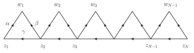
Figure 2: The diagrammatic representation for the kernel $\Lambda_{N}^{(x_{1},\bar{x}_{1})}(z_{1},\ldots,z_{N}|w_{1},\ldots,w_{N-1})$ (up to factor $r_{N}(x,\bar{x})$). The arrow with index $\alpha$ from $z$ to $w$ stands for $(w-z)^{-\alpha}(\bar{w}-\bar{z})^{\bar{\alpha}}$. The indices are given by the following expressions: $\alpha=1-s-ix$, $\beta=1-s+ix$, $\gamma=2s-1$.

Now it is easy to see that the eigenfunctions of the operators $B_{N}(u)$ and $\bar{B}_{N}(\bar{u})$ have the form

$$\Psi_{B}({\boldsymbol{x}}|\boldsymbol{z})=|p|^{N-1}\,\Lambda_{N}{(\boldsymbol{x}_{1})}\,\Lambda_{N-1}{(\boldsymbol{x}_{2})}\ldots\Lambda_{2}{(\boldsymbol{x}_{N-1})}\,e^{ipz_{1}+i\bar{p}\bar{z}_{1}}\,.$$ (41)

Each operator $\Lambda_{k}{(\boldsymbol{x}_{k})}$ maps a function of $k-1$ variables to a function of $k$ variables. Thus the product of the operators in (41) maps the function of one variable, $e^{ipz_{1}+i\bar{p}\bar{z}_{1}}$, to a function of $N-$variables. In order to obtain the conventional normalization of the eigenfunctions we included the prefactor $|p|^{N-1}$ in the definition (41). Taking into account Eq. (36) and using that $B_{1}(u)=S_{1}=-\partial_{z_{1}}$ one obtains

$$B_{N}(u)\,\Psi_{B}({\boldsymbol{x}}|\boldsymbol{z})=p\prod_{k=1}^{N-1}(u-x_{k})\,\Psi_{B}({\boldsymbol{x}}|\boldsymbol{z})\,,\qquad\bar{B}_{N}(\bar{u})\,\Psi_{B}({\boldsymbol{x}}|\boldsymbol{z})=\bar{p}\prod_{k=1}^{N-1}(\bar{u}-\bar{x}_{k})\,\Psi_{B}({\boldsymbol{x}}|\boldsymbol{z})\,.$$ (42)

Note also that due to the exchange relation (40) the eigenfunctions are symmetric functions of the parameters $(\boldsymbol{x_{1}},\ldots\boldsymbol{x}_{N-1})$.

Let us figure out which are the possible values of the variables $(\boldsymbol{x_{1}},\ldots\boldsymbol{x}_{N-1})$.. By construction the variables $(\{x_{1},\bar{x}_{1}\},\ldots\{x_{N-1},\bar{x}_{N-1}\})$ satisfy the restriction

$$(s+ix_{k})-(\bar{s}-i\bar{x}_{k})=i(x_{k}-\bar{x}_{k})+n_{s}\in\mathbb{Z}$$ (43)

for all $k$. Further, the operator $B_{N}(u)$ is a hermitian adjoint of $\bar{B}_{N}(\bar{u})$, $\bar{B}_{N}(\bar{u})=(B_{N}(u))^{\dagger}$, provided that $u^{*}=\bar{u}$. It results in the following relation for the eigenvalues

$$\left(\prod_{k=1}^{N-1}(u-x_{k})\right)^{*}=\prod_{k=1}^{N-1}(u^{*}-\bar{x}_{k})$$

that, in its turn, implies that $x_{k}^{*}=\bar{x}_{k}$. Together with the condition (43) it results in the following parametrization [22]

$$x_{k}=-\frac{in_{k}}{2}+\nu_{k}\,,\qquad\bar{x}_{k}=\frac{in_{k}}{2}+\nu_{k}\,,$$ (44)

where $\nu_{k}$ is real and $n_{k}$ is integer (if $n_{s}$ is integer) or half-integer (if $n_{s}$ is half-integer).

3.2 $A-$system

The construction of the eigenfunctions of the operator $A_{N}(u)$ goes along the same lines. Let us apply both sides of the first of Eqs. (3) to a function $\Psi$ which depends on $z_{N}$ and $\bar{z}_{N}$ in the specific way, $\Psi=[z_{N}]^{i(u_{1}-v)-1}\Psi_{N-1}(z_{1},\ldots,z_{N-1})$. The second term ($\sim B_{N-1}(u)$) on the r.h.s. of this equation vanishes so that one obtains

$$A_{N}(u)\boldsymbol{\Lambda}_{N}(u,v)[z_{N}]^{i(u_{1}-v)-1}\Psi_{N-1}=(u+is-u_{1}+v-i)\boldsymbol{\Lambda}_{N}(u,v)A_{N-1}(u)[z_{N}]^{i(u_{1}-v)-1}\Psi_{N-1}\,.$$ (45)

Taking into account explicit expression for the operator $\mathcal{R}_{N-1,N}^{(2)}$, Eq. (2.2), it is easy to verify that $\boldsymbol{\Lambda}_{N}(u,v)z_{N}=z_{N}\boldsymbol{\Lambda}_{N}(u,v)$. Finally, substituting $v=u-x$ and multiplying both sides of (45) by the normalization factor $r_{N}(x,\bar{x})$ one obtains

$$A_{N}(u)\,\tilde{\Lambda}_{N}{(x,\bar{x})}=(u-x)\,\tilde{\Lambda}_{N}{(x,\bar{x})}\,A_{N-1}(u)\,.$$ (46)

The operator

$$\tilde{\Lambda}_{N}{(\boldsymbol{x})}=[z_{N}^{ix-s}]\,\Lambda_{N}{(\boldsymbol{x})}\equiv z_{N}^{ix-s}\,\bar{z}_{N}^{i\bar{x}-\bar{s}}\,\Lambda_{N}{(\boldsymbol{x})}$$ (47)

maps a function of $N-1$ variables to a function of $N-$variables. The diagrammatic representation for the kernel of the operator $\tilde{\Lambda}_{N}{(\boldsymbol{x}_{1})}$ is shown in Fig. 3.

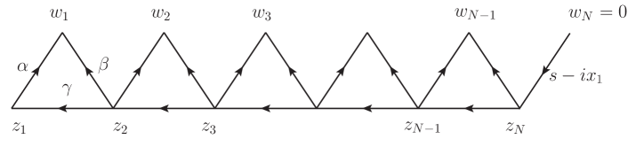
Figure 3: The diagrammatic representation for the kernel $\tilde{\Lambda}_{N}^{(x_{1},\bar{x}_{1})}(z_{1},\ldots,z_{N}|w_{1},\ldots,w_{N-1})$ (up to factor $r_{N}(x,\bar{x})$). The indices are given by the following expressions: $\alpha=1-s-ix$, $\beta=1-s+ix$, $\gamma=2s-1$.

The eigenfunctions of the operators $A_{N}(u)$, $\bar{A}_{N}(\bar{u})$ are constructed using the same scheme as the eigenfunctions of $B_{N}$ operators. Namely,

$$\Psi_{A}({\boldsymbol{x}}|\boldsymbol{z})=\tilde{\Lambda}_{N}{(\boldsymbol{x}_{1})}\ \ldots\tilde{\Lambda}_{2}{(\boldsymbol{x}_{N-1})}\tilde{\Lambda}_{1}{(\boldsymbol{x}_{N})}=\tilde{\Lambda}_{N}{(\boldsymbol{x}_{1})}\,\ldots\tilde{\Lambda}_{2}{(\boldsymbol{x}_{N-1})}[z_{1}]^{ix_{1}-s}\,.$$ (48)

The diagrammatic representation for $\Psi_{A}({\boldsymbol{x}}|\boldsymbol{z})$ is shown in Fig. 3. Evidently this function satisfies Eqs. (2.1). The eigenfunction (48) is symmetric under permutations of variables, $\boldsymbol{x}_{k}\leftrightarrow\boldsymbol{x}_{j}$. This property follows from the exchange relation

$$\tilde{\Lambda}_{N}{(\boldsymbol{x}_{1})}\,\tilde{\Lambda}_{N-1}{(\boldsymbol{x}_{2})}=\tilde{\Lambda}_{N}{(\boldsymbol{x}_{2})}\,\tilde{\Lambda}_{N-1}{(\boldsymbol{x}_{1})}\,$$ (49)

which can be proven using the same diagrammatic technique.

3.3 $C$ and $D$ systems

The eigenfunctions of the operators $D_{N}$ and $C_{N}$ are related to those of $A_{N}$ and $B_{N}$ by an inversion transformation. The inversion operator $J$,

$$[{J}\varphi](z_{1},\ldots,z_{N})=\psi(z_{1},\ldots,z_{N})=\prod_{k=1}^{N}z_{k}^{-2s}\bar{z}_{k}^{-2\bar{s}}\varphi\left(\frac{1}{z_{1}},\ldots,\frac{1}{z_{N}}\right)\,,$$ (50)

generates the following transformation of the $sl(2)$ algebra

$${J}\,S^{(k)}_{\pm}\,{J}=S^{(k)}_{\mp}\,,\quad{J}\,S^{(k)}_{0}\,{J}=-S^{(k)}_{0}\,,\quad{J}\,\bar{S}^{(k)}_{\pm}\,{J}=\bar{S}^{(k)}_{\mp}\,,\quad{J}\,\bar{S}^{(k)}_{0}\,{J}=-\bar{S}^{(k)}_{0}\,.$$ (51)

The $L-$operators (and hence monodromy matrices) transform under the inversion as follows

$${J}\,L_{k}(u)\,{J}=\sigma_{1}\,L_{k}(u)\,\sigma_{1}\,, {J}\,\bar{L}_{k}(\bar{u})\,{J}=\sigma_{1}\,\bar{L}_{k}(\bar{u})\,\sigma_{1}\,,$$

$${J}\,T_{N}(u)\,{J}=\sigma_{1}\,T_{N}(u)\,\sigma_{1}\,, {J}\,\bar{T}_{N}(\bar{u})\,{J}=\sigma_{1}\,\bar{T}_{N}(\bar{u})\,\sigma_{1}\,,$$ (52)

where $\sigma_{1}$ is the Pauli matrix. From Eqs. (52) one immediately derives

$${J}\,A_{N}(u)=D_{N}(u)\,{J}\,, {J}\,\bar{A}_{N}(\bar{u})=\bar{D}_{N}(\bar{u})\,{J}\,,$$

$${J}\,B_{N}(u)=C_{N}(u)\,{J}\,, {J}\,\bar{B}_{N}(\bar{u})=\bar{C}_{N}(\bar{u})\,{J}\,.$$ (53)

Thus the eigenfunctions of the $D_{N}(u),\bar{D}_{N}(\bar{u})$ ($C_{N}(u),\bar{C}_{N}(\bar{u})$) commutative family are related to those of $A_{N}(u),\bar{A}_{N}(\bar{u})$ ($B_{N}(u),\bar{B}_{N}(\bar{u})$) by inversion. Namely, for the $D-$system one obtains

$$\Psi_{D}({\boldsymbol{x}}|\boldsymbol{z})={J}\,\Psi_{A}({\boldsymbol{x}}|\boldsymbol{z})=\widehat{\Lambda}_{N}{(x_{1},\bar{x}_{1})}\,\widehat{\Lambda}_{N-1}{(x_{2},\bar{x}_{2})}\ldots\widehat{\Lambda}_{2}{(x_{N-1},\bar{x}_{N-1})}\,\widehat{\Lambda}_{1}{(x_{N},\bar{x}_{N})}\,,$$ (54)

where $\widehat{\Lambda}_{k}{(x,\bar{x})}=z_{1}^{-ix-s}\,\bar{z}_{1}^{-ix-s}\,\Lambda_{k}{(x,\bar{x})}$. In turn, for the $C-$system one gets

$$\Psi_{C}({\boldsymbol{x}}|\boldsymbol{z}) = {J}\,\Psi_{B}({\boldsymbol{x}}|\boldsymbol{z})$$ (55)

$$= |p|^{N-1}\,\bar{\Lambda}_{N}{(x_{1},\bar{x}_{1})}\,\bar{\Lambda}_{N-1}{(x_{2},\bar{x}_{2})}\ldots\bar{\Lambda}_{2}{(x_{N-1},\bar{x}_{N-1})}z_{1}^{-2s}\bar{z}_{1}^{-2\bar{s}}e^{ip/z_{1}+i\bar{p}/\bar{z}_{1}}\,,$$

with $\bar{\Lambda}_{k}{(x,\bar{x})}=z_{1}^{-ix-s}\,\bar{z}_{1}^{-i\bar{x}-\bar{s}}\,z_{k}^{ix-s}\,\bar{z}_{k}^{i\bar{x}-\bar{s}}\,\Lambda_{k}{(x,\bar{x})}$.

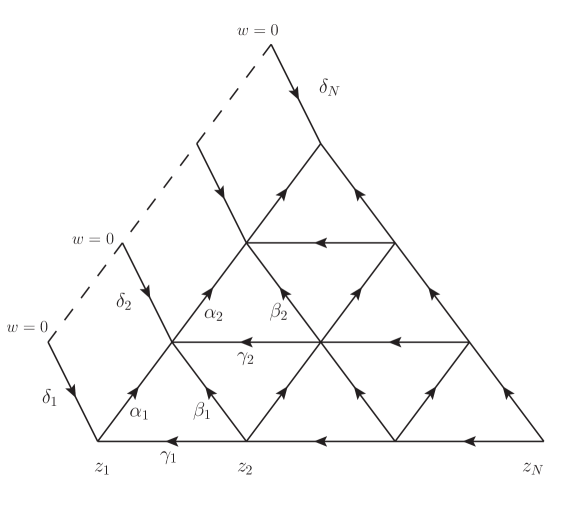
Figure 4: The diagrammatic representation of the eigenfunction $\Psi_{D}(\boldsymbol{x}|\boldsymbol{z})$. Here $\alpha_{k}=1-s-ix_{k}$, $\beta_{k}=1-s+ix_{k}$, $\gamma_{k}=2s-1$ and $\delta_{k}=s+ix_{k}$. The dashed line stands for the point $w=0$.

4 Scalar products and Sklyanin’s measure

The functions $\Psi_{S}({\boldsymbol{x}}|\boldsymbol{z})$, $S=A,B,C,D$, being eigenfunctions of the self-adjoint operators form a complete orthonormal basis in the Hilbert space $\mathbb{H}_{N}$. Arbitrary function $\Phi\in\mathbb{H}_{N}$ can be expanded in this basis as follows

$$\Phi(z)=\int\mathcal{D}_{S}\boldsymbol{x}\,\boldsymbol{\mu}_{S}(\boldsymbol{x})\,C_{S}(\boldsymbol{x})\,\Psi_{S}({\boldsymbol{x}}|\boldsymbol{z})\,.$$ (56)

The symbol $\mathcal{D}_{S}\boldsymbol{x}$ stands for

$$\mathcal{D}_{A(D)}\boldsymbol{x}=\prod_{k=1}^{N}\left(\sum_{n_{k}=-\infty}^{\infty}\int_{-\infty}^{\infty}d\nu_{k}\right)\,,\quad\mathcal{D}_{B(C)}\boldsymbol{x}=d^{2}p\,\prod_{k=1}^{N-1}\left(\sum_{n_{k}=-\infty}^{\infty}\int_{-\infty}^{\infty}d\nu_{k}\right)\,.$$ (57)

Depending on the value of the spin in the quantum space, $n_{s}=s-\bar{s}$, the sum over $n_{k}$ goes over all integers (integer $n_{s}$) or half-integers (half-integer $n_{s}$). The weight function $\boldsymbol{\mu}_{S}(\boldsymbol{x})$ is the so-called Sklyanin’s measure and the function $C_{S}(\boldsymbol{x})$ is given by the scalar product

$$C_{S}(\boldsymbol{x})=\langle{\Psi_{S}({\boldsymbol{x}}|\boldsymbol{z})|\Phi(\boldsymbol{z})}\rangle\,.$$ (58)

Sklyanin’s measure $\boldsymbol{\mu}_{S}(\boldsymbol{x})$ is related to the scalar product of the eigenfunctions

$$\langle{\Psi_{S}({\boldsymbol{x}^{\prime}}|\boldsymbol{z})|\Psi_{S}({\boldsymbol{x}}|\boldsymbol{z})}\rangle=\boldsymbol{\mu}^{-1}_{S}(\boldsymbol{x})\,\delta_{S}(\boldsymbol{x}-\boldsymbol{x}^{\prime})\,.$$ (59)

Here the delta function $\delta_{S}(\boldsymbol{x}-\boldsymbol{x}^{\prime})$ is defined as follows:

• For $S=A,D$

  $$\delta_{S}(\boldsymbol{x}-\boldsymbol{x}^{\prime})=\frac{1}{N!}\sum_{S_{N}}\delta(\boldsymbol{x}_{1}-\boldsymbol{x}^{\prime}_{k_{1}})\ldots\delta(\boldsymbol{x}_{N}-\boldsymbol{x}^{\prime}_{k_{N}})\,.$$ (60)

• For $S=B,C$

  $$\delta_{S}(\boldsymbol{x}-\boldsymbol{x}^{\prime})=\frac{1}{(N-1)!}\delta^{2}(\vec{p}-\vec{p}^{\prime})\sum_{S_{N-1}}\delta(\boldsymbol{x}_{1}-\boldsymbol{x}^{\prime}_{k_{1}})\ldots\delta(\boldsymbol{x}_{N-1}-\boldsymbol{x}^{\prime}_{k_{N-1}})\,.$$ (61)

In above expressions summation goes over all permutations of $N$ and $N-1$ elements, respectively and

$$\delta(\boldsymbol{x}_{k}-\boldsymbol{x}^{\prime}_{m})\equiv\delta_{n_{k}n^{\prime}_{m}}\delta(\nu_{k}-\nu^{\prime}_{m})$$ (62)

The calculation of the scalar product (59) is based on the following exchange relations for $\Lambda$ operators

$$\Lambda_{k}^{\dagger}(\boldsymbol{x}^{\prime}_{k})\,\Lambda_{k}(\boldsymbol{x}_{k}) = \alpha(\boldsymbol{x}_{k},\boldsymbol{x}^{\prime}_{k})\,\Lambda_{k-1}(\boldsymbol{x}_{k})\Lambda_{k-1}^{\dagger}(\boldsymbol{x}^{\prime}_{k})\,,$$ (63a)

$$\tilde{\Lambda}_{k}^{\dagger}(\boldsymbol{x}^{\prime}_{k})\,\tilde{\Lambda}_{k}(\boldsymbol{x}_{k}) = \alpha(\boldsymbol{x}_{k},\boldsymbol{x}^{\prime}_{k})\,\tilde{\Lambda}_{k-1}(\boldsymbol{x}_{k})\tilde{\Lambda}_{k-1}^{\dagger}(\boldsymbol{x}^{\prime}_{k})\,,$$ (63b)

where it is assumed that $\boldsymbol{x}^{\prime}_{k}\neq\boldsymbol{x}_{k}$ and

$$\alpha(\boldsymbol{x}_{k},\boldsymbol{x}^{\prime}_{k})=\frac{\pi^{2}}{(x_{k}-x^{\prime}_{k})(\bar{x}_{k}-\bar{x}^{\prime}_{k})}\,.$$ (63bl)

The relations (63a), (63b) can be proven diagrammatically. Namely, one can show that the diagrams on the l.h.s and r.h.s. of Eq. (63b),(63a) can be brought to the same form after a certain sequence of transformations. The transformations relevant for Eq. (63a) are shown schematically in Fig. 5.

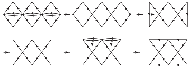
Figure 5: An illustration to the diagrammatic proof of the exchange relation (63a).

This technique and its application to the analysis of the $SL(2,\mathbb{C})$ spin chains was discussed at length in Ref. [22]. Therefore we will not go in much detail here and only comment briefly on the sequence of transformations shown in Fig. 5. i) The right-most diagram in the first row is a diagrammatic representation for the kernel $\Lambda_{k}^{\dagger}(\boldsymbol{x}^{\prime}_{k})\,\Lambda_{k}(\boldsymbol{x}_{k})$ ($k=3$). The lines inside the rhombuses have indices $2s-1$ and $1-2s$ and therefore cancel (their product is equal to $1$). ii) One integrates over the right-most and leftmost vertices using the chain integration rule (A.139). iii) The left-most vertical line is moved with the help of the cross identity (• ‣ A) to the right where it cancels with leftmost vertical line resulting in the first diagram in the second line iv) One inserts unity given by the product of two lines with indices $(1-2s)$ (upper line) and $(2s-1)$ (lower line) and moves lower lines down using cross identity (• ‣ A). v) One flips arrows on the lines (except the horizontal ones). The last diagram in the second row coincides up to prefactor with a diagram for the kernel of the product of the opartors $\Lambda_{k-1}(\boldsymbol{x}_{k})\Lambda_{k-1}^{\dagger}(\boldsymbol{x}^{\prime}_{k})$ ($k=3$). Collecting all factors which arise during these transformations one arrives at Eq. (63a).

The proof of the second relation, Eq. (63b), goes along the same lines and we will not discuss it.

Let us come back to the calculation of the scalar product (59). Using the representations (41) and (48) for the eigenfunctions and making use of the exchange relations (63b), (63a) one can bring the scalar product (59) to the form

$$\langle{\Psi_{A}({\boldsymbol{x}^{\prime}}|\boldsymbol{z})|\Psi_{A}({\boldsymbol{x}}|\boldsymbol{z})}\rangle = M_{A}(\boldsymbol{x},\boldsymbol{x}^{\prime})\,\tilde{\Lambda}_{1}^{\dagger}(\boldsymbol{x}^{\prime}_{N})\tilde{\Lambda}_{1}(\boldsymbol{x}_{1})\,\tilde{\Lambda}_{1}^{\dagger}(\boldsymbol{x}^{\prime}_{N-1})\tilde{\Lambda}_{1}(\boldsymbol{x}_{2})\ldots\tilde{\Lambda}_{1}^{\dagger}(\boldsymbol{x}^{\prime}_{1})\tilde{\Lambda}_{1}(\boldsymbol{x}_{N})\,,$$ (63bma)

$$\langle{\Psi_{B}({\boldsymbol{x}^{\prime}}|\boldsymbol{z})|\Psi_{B}({\boldsymbol{x}}|\boldsymbol{z})}\rangle = M_{B}(\boldsymbol{x},\boldsymbol{x}^{\prime})\,$$ (63bmb)

$$\times \langle E_{p^{\prime}}(z)\big{|}\Lambda_{2}^{\dagger}(\boldsymbol{x}^{\prime}_{N-1})\Lambda_{2}(\boldsymbol{x}_{1})\,\Lambda_{2}^{\dagger}(\boldsymbol{x}^{\prime}_{N-2})\Lambda_{2}(\boldsymbol{x}_{2})\ldots\Lambda_{2}^{\dagger}(\boldsymbol{x}^{\prime}_{1})\Lambda_{2}(\boldsymbol{x}_{N-1})\big{|}E_{p}(z)\rangle\,,$$

where $E_{p}(z)=e^{ipz+i\bar{p}\bar{z}}.$ In order to use the exchange relations one has to assume that $\boldsymbol{x}^{\prime}_{N-k}\neq\boldsymbol{x}_{j}$ for $j\neq k$ in the product (63bma) and $\boldsymbol{x}^{\prime}_{N-1-k}\neq\boldsymbol{x}_{j}$ for $j\neq k$ in (63bmb). In order to calculate the scalar products for other arrangements of the variables one has to use symmetry properties of the eigenfunctions. The functions $M_{S}(\boldsymbol{x},\boldsymbol{x}^{\prime})$ take the form

$$M_{A}(\boldsymbol{x},\boldsymbol{x}^{\prime})=\prod_{{j+k\leq N}}\alpha(\boldsymbol{x}_{j},\boldsymbol{x}^{\prime}_{k})\,,\quad M_{B}(\boldsymbol{x},\boldsymbol{x}^{\prime})=|pp^{\prime}|^{N-1}\prod_{j+k\leq N-1}\alpha(\boldsymbol{x}_{j},\boldsymbol{x}^{\prime}_{k})\,.$$ (63bmbn)

The calculation of the product $\tilde{\Lambda}_{1}^{\dagger}\tilde{\Lambda}_{1}$ is straightforward

$$\tilde{\Lambda}_{1}^{\dagger}(\boldsymbol{x}^{\prime})\tilde{\Lambda}_{1}(\boldsymbol{x})=\int d^{2}z{z^{-1+i(x-x^{\prime})}\bar{z}^{-1+i(\bar{x}-\bar{x}^{\prime})}}=2\pi^{2}\,\delta_{nn^{\prime}}\,\delta(\nu-\nu^{\prime})=2\pi^{2}\,\delta(\boldsymbol{x}-\boldsymbol{x}^{\prime})\,.$$ (63bmbo)

Taking into account Eqs. (63bl) and (63bma) we obtain for the measure $\boldsymbol{\mu}_{A}(\boldsymbol{x})$

$$\boldsymbol{\mu}_{A}(\boldsymbol{x})=(2\pi)^{-N}\pi^{-N^{2}}\prod_{k<j}(x_{k}-x_{j})(\bar{x}_{k}-\bar{x}_{j})=(2\pi)^{-N}\pi^{-N^{2}}\prod_{j<k}\left((\nu_{k}-\nu_{j})^{2}+\frac{1}{4}(n_{k}-n_{j})^{2}\right)\,.$$ (63bmbp)

Further, Eq. (63bmb) can be simplified with the help of the following relation

$$\Lambda_{2}^{\dagger}(\boldsymbol{x}^{\prime})\,\Lambda_{2}(\boldsymbol{x})e^{i(pz+\bar{p}\bar{z})}=e^{i(pz+\bar{p}\bar{z})}|p|^{-2}\,2\pi^{4}\,\delta(\boldsymbol{x}-\boldsymbol{x}^{\prime})\,.$$ (63bmbq)

In order to verify Eq. (63bmbq) one can calculate a diagram which corresponds to the l.h.s of this equation. It can be done easily by going over to the momentum representation (see also Ref. [22]). Collecting all factors one gets for the measure

$$\boldsymbol{\mu}_{B}(\boldsymbol{x}) = 2(2\pi)^{-N}\pi^{-N^{2}}\prod_{k<j\leq N-1}(x_{k}-x_{j})(\bar{x}_{k}-\bar{x}_{j})$$ (63bmbr)

$$= 2(2\pi)^{-N}\pi^{-N^{2}}\prod_{j<k\leq N-1}\left((\nu_{k}-\nu_{j})^{2}+\frac{1}{4}(n_{k}-n_{j})^{2}\right)\,.$$

We would like to stress here that the completeness of the constructed orthonormal systems

$$\int\mathcal{D}_{S}\boldsymbol{x}\,\boldsymbol{\mu}_{S}(\boldsymbol{x})\,\Psi_{S}({\boldsymbol{x}}|\boldsymbol{z})\,\left(\Psi_{S}({\boldsymbol{x}}|\boldsymbol{z}^{\prime})\right)^{\dagger}=\prod_{k=1}^{N}\delta^{2}(\vec{z}_{k}-\vec{z}^{\prime}_{k})$$ (63bmbs)

deserves a separate study. For $N=1,2$ Eq. (63bmbs) can be easily checked by elementary methods, see e.g. [33]. As to general $N$ we hope that the method developed in Ref. [32] for the quantum Toda chain could prove useful for verifying the completeness condition (63bmbs).

Closing this section we want to mention that the basis of eigenfunctions of the elements of the momodromy matrix proves to be useful in applications, e.g. for studies of form factors [43, 38, 35, 49] and correlation functions [26, 44]. The basis of eigenfunctions of $B-$operator plays a prominent role in analysis of the closed spin chains since it determines so-called Sklyanin’s representation of Separated Variables [7]. The applications of the SoV methods for particular models can be found in Refs. [9, 11, 30, 22, 31, 38, 35].

5 Baxter’s operators

The method of Baxter’s operators [14] provides an alternative to the conventional Algebraic Bethe Ansatz. Let operators $\mathcal{Q}(u)$ form a commutative family, $[\mathcal{Q}(u),\mathcal{Q}(v)]=0$. The operator $\mathcal{Q}(u)$ is called Baxter operator if it also commutes with integral of motions of the model (including Hamiltonian) and satisfies a certain finite-difference equation (Baxter equation). Provided that the analytic properties of the eigenvalues as functions of the spectral parameter $u$ are known one can obtain them by solving the Baxter equation. It turns out that such fundamental objects as transfer matrices and the Hamiltonian can be expressed in terms of $\mathcal{Q}$ operators in a rather simple way. For the closed $SL(2,\mathbb{C})$ spin chains the Baxter operators were constructed in Ref. [22]. In this section we construct the set of Baxter operators $\mathcal{Q}_{S}(\boldsymbol{u})\equiv\mathcal{Q}_{S}(u,\bar{u})$,  $S=A,B,C,D$,  such that they commute with the corresponding elements of the monodromy matrices, ${T}_{N}(v)$, $\bar{{T}}_{N}(\bar{v})$,

$$[\mathcal{Q}_{A}(\boldsymbol{u}),\ A_{N}(v)] = [\mathcal{Q}_{A}(\boldsymbol{u}),\ \bar{A}_{N}(\bar{v})]=0\,,$$

$${}[\mathcal{Q}_{D}(\boldsymbol{u}),\ D_{N}(v)] = [\mathcal{Q}_{D}(\boldsymbol{u}),\ \bar{D}_{N}(\bar{v})]=0\,,$$ (63bmbt)

etc. We also derive the difference equations which these operators satisfy.

Figure 6: The diagrammatic representation of the operator $\mathcal{T}_{\boldsymbol{s}_{0}}(\boldsymbol{u})=\mathcal{Q}_{-}(u+i(1-s_{0}))\mathcal{Q}_{+}(u+is_{0})$. Here the black blobs stand for the integration vertices, the gray blobs indicate $z_{0}=0$. The indices are the following $\alpha=1-s-iu^{+}$, $\beta=1-s+iu^{+}$, $\gamma=s+iu^{-}$, $\delta=s-iu^{-}$ and $u^{-}=u+i(1-s_{0})$, $u^{+}=u+is_{0}$

Let us define an operator

$$\mathbb{T}_{\boldsymbol{s}_{0}}(\boldsymbol{u})=\mathcal{R}_{\boldsymbol{s}_{0}\boldsymbol{s}_{1}}(\boldsymbol{u})\,\mathcal{R}_{\boldsymbol{s}_{0}\boldsymbol{s}_{2}}(\boldsymbol{u})\ldots\mathcal{R}_{\boldsymbol{s}_{0}\boldsymbol{s}_{N}}(\boldsymbol{u})\,$$ (63bmbu)

which acts on the tensor product $\mathbb{V}_{0}\otimes\mathbb{H}_{N}$, where $\mathbb{V}_{0}=L_{2}(\mathbb{C})$ is an auxiliary space and $\mathbb{H}_{N}$ is the quantum space of the model, $\mathbb{H}_{N}=\otimes_{k=1}^{N}\mathbb{V}_{k}$. As usual it is assumed that the operator $\mathcal{R}_{\boldsymbol{s}_{0}\boldsymbol{s}_{k}}(\boldsymbol{u})$, see Eq. (2.2), acts nontrivially on the tensor product $\mathbb{V}_{0}\otimes\mathbb{V}_{k}$. It follows from the relation (2.2) that this operator obeys the following commutation relation

$$\mathbb{T}_{\boldsymbol{s}_{0}}(\boldsymbol{u})\,{T}_{N}(v)\,L_{s_{0}}(v-u)=L_{s_{0}}(v-u)\,{T}_{N}(v)\,\mathbb{T}_{\boldsymbol{s}_{0}}(\boldsymbol{u})\,,$$ (63bmbv)

where ${T}_{N}(v)$ is the monodromy matrix (9) and $L_{s_{0}}$ is the $L-$operator which acts on $\mathbb{V}_{0}\otimes\mathbb{C}^{2}$. The products ${T}_{N}(v)\,L_{s_{0}}(v-u)$ and $L_{s_{0}}(v-u)\,{T}_{N}(v)\,$ are $2\times 2$ matrices so that Eq. (63bmbv) reads in explicit form

$$\mathbb{T}_{\boldsymbol{s}_{0}}(\boldsymbol{u})\left(\begin{array}[]{cc}A_{N}(v)&B_{N}(v)\\ C_{N}(v)&D_{N}(v)\end{array}\right)\left(\begin{array}[]{cc}v-u+z_{0}\partial_{z_{0}}+s_{0}&-\partial_{z_{0}}\\ z_{0}^{2}\partial_{z_{0}}+2s_{0}z_{0}&v-u-z_{0}\partial_{z_{0}}-s_{0}\end{array}\right)=$$ (63bmca)

$$=\left(\begin{array}[]{cc}v-u+z_{0}\partial_{z_{0}}+s_{0}&-\partial_{z_{0}}\\ z_{0}^{2}\partial_{z_{0}}+2s_{0}z_{0}&v-u-z_{0}\partial_{z_{0}}-s_{0}\end{array}\right)\left(\begin{array}[]{cc}A_{N}(v)&B_{N}(v)\\ C_{N}(v)&D_{N}(v)\end{array}\right)\mathbb{T}_{\boldsymbol{s}_{0}}(\boldsymbol{u})\,.$$ (63bmcf)

The equation involving the matrix element $(2,2)$ has the form

$$\mathbb{T}_{\boldsymbol{s}_{0}}(\boldsymbol{u})\Big{(}D_{N}(v)(v-u-z_{0}\partial_{z_{0}}-s_{0})-C_{N}(v)\partial_{z_{0}}\Big{)}=$$

$$=\Big{(}(v-u-z_{0}\partial_{z_{0}}-s_{0})D_{N}(v)+(z_{0}^{2}\partial_{z_{0}}+2s_{0}z_{0})B_{N}(v)\Big{)}\mathbb{T}_{\boldsymbol{s}_{0}}(\boldsymbol{u}).$$ (63bmcg)

The l.h.s and r.h.s. of this equation are operators that act on the space of functions of $N+1$ variables, $\psi(z_{0},z_{1},\ldots,z_{N})$. Applying both sides of Eq. (5) to the function $f=f(z_{1},\ldots,z_{N})$ which does not depend on $z_{0}$ and sending $z_{0}\to 0$ in the result one obtains

$$\mathbb{T}_{\boldsymbol{s}_{0}}(\boldsymbol{u})\,D_{N}(v)f=D_{N}(v)\,\mathbb{T}_{\boldsymbol{s}_{0}}(\boldsymbol{u})f\Big{|}_{z_{0}=0}\,.$$ (63bmch)

Hence the operator $\mathcal{T}_{\boldsymbol{s}_{0}}(\boldsymbol{u})$ which is defined on the space of functions of $N$ variables

$$[\mathcal{T}_{\boldsymbol{s}_{0}}(\boldsymbol{u})f](z_{1},\ldots,z_{N})=[\mathbb{T}_{\boldsymbol{s}_{0}}(\boldsymbol{u})f](z_{0},z_{1},\ldots,z_{N})|_{z_{0}\to 0}$$ (63bmci)

commutes with the element $D_{N}(v)$ (and $\bar{D}_{N}(\bar{v})$) of the monodromy matrix

$$[\mathcal{T}_{\boldsymbol{s}_{0}}(\boldsymbol{u}),D_{N}(v)]=[\mathcal{T}_{\boldsymbol{s}_{0}}(\boldsymbol{u}),\bar{D}_{N}(\bar{v})]=0\,.$$ (63bmcj)

The kernel of the integral operator $\mathcal{T}_{\boldsymbol{s}_{0}}(\boldsymbol{u})$ is related to the kernel of the operator $\mathbb{T}_{\boldsymbol{s}_{0}}(\boldsymbol{u})$ as follows

$$\mathcal{T}_{\boldsymbol{s}_{0}}(\boldsymbol{u})(z_{1},\ldots,z_{N}|w_{1},\ldots,w_{N})=\int d^{2}w\,\mathbb{T}_{\boldsymbol{s}_{0}}(\boldsymbol{u})(0,z_{1},\ldots,z_{N}|w,w_{1},\ldots,w_{N})\,.$$ (63bmck)

The operator $\mathcal{T}_{\boldsymbol{s}_{0}}(\boldsymbol{u})$ depends on the spins $s_{0},\bar{s}_{0}$ in the auxiliary space and the spectral parameters $u,\bar{u}$ and thus can be considered as an analog of a transfer matrix. The proof of commutativity

$$[\mathcal{T}_{\boldsymbol{s}_{0}}(\boldsymbol{u}),\mathcal{T}_{\boldsymbol{s}_{0^{\prime}}}(\boldsymbol{v})]=0\,.$$ (63bmcl)

is given in Appendix B.

It is known that the transfer matrices for the $SL(2,\mathbb{C})$ spin chains factorize into the product of two Baxter $\mathcal{Q}$ operators [22]. The same holds true in the case under consideration. The operator $\mathcal{T}_{\boldsymbol{s}_{0}}(\boldsymbol{u})$ can be represented as product of two operators

$$\mathcal{T}_{\boldsymbol{s}_{0}}(\boldsymbol{u})=\mathcal{Q}_{-}(\boldsymbol{u}+i(1-\boldsymbol{s}_{0}))\,\mathcal{Q}_{+}(\boldsymbol{u}+i\boldsymbol{s}_{0}).$$ (63bmcm)

The kernel of $\mathcal{T}_{\boldsymbol{s}_{0}}(\boldsymbol{u})$ and its representation in the factorized form is shown in Fig. 6. While the “transfer matrix” $\mathcal{T}_{\boldsymbol{s}_{0}}(\boldsymbol{u})$ depends on two sets of variables: the spin $\boldsymbol{s}_{0}=(s_{0},\bar{s}_{0})$ and the spectral parameter $\boldsymbol{u}=(u,\bar{u})$, each of the operators $\mathcal{Q}_{\pm}$ depends only on one variable. In the explicit form the kernels of the operators $\mathcal{Q}_{\pm}(\boldsymbol{u}))$ are given by the following expressions

$$\mathcal{Q}_{-}(\boldsymbol{u})(z_{1},\ldots,z_{N}|w_{1},\ldots,w_{N}) = \prod_{k=1}^{N}[z_{k}-w_{k-1}]^{-s-iu}[z_{k}-w_{k}]^{-s+iu}[w_{k}-w_{k-1}]^{2s-1}\,,$$

$$\mathcal{Q}_{+}(\boldsymbol{u})(z_{1},\ldots,z_{N}|w_{1},\ldots,w_{N}) = \prod_{k=1}^{N}[w_{k}-z_{k-1}]^{-1+s+iu}[w_{k}-z_{k}]^{-1+s-iu}[z_{k}-z_{k-1}]^{1-2s}\,,$$ (63bmcn)

where $w_{0}=z_{0}=0$. The requirement for the kernel to be a single-valued function on the complex plane results in the following restriction on the spectral parameters

$$(s-\bar{s})+i(u-\bar{u})=n_{s}+i(u-\bar{u})=n\in\mathbb{Z}\,.$$ (63bmco)

Thus the spectral parameters $u,\bar{u}$ have the form (44) where $\nu$ takes now complex values.

Taking into account Eq. (A.143) one easily derives that operators $\mathcal{Q}_{\pm}$ satisfy the following normalization conditions

$$\mathcal{Q}_{-}(i(1-\boldsymbol{s})+\epsilon)=\left(\frac{\pi}{i\epsilon}\right)^{N}\Big{(}\hbox{{1}\kern-2.5pt\hbox{l}}+O(\epsilon)\Big{)}\,,\qquad\mathcal{Q}_{+}(-i\boldsymbol{s}-\epsilon)=\left(\frac{\pi}{i\epsilon}\right)^{N}\Big{(}\hbox{{1}\kern-2.5pt\hbox{l}}+O(\epsilon)\Big{)}\,.$$ (63bmcp)

Eqs. (63bmcp) allow one to represent the operators $\mathcal{Q}_{\pm}$ as certain limits of the operator $\mathcal{T}_{\boldsymbol{s}_{0}}(\boldsymbol{u})$, e.g.

$$\lim_{\epsilon\to 0}(i\epsilon)^{N}\mathcal{T}_{i\boldsymbol{u}-\boldsymbol{s}+i\epsilon}(\boldsymbol{u})=\pi^{N}\mathcal{Q}_{-}(2\boldsymbol{u}+i(1-\boldsymbol{s}))\,.$$ (63bmcq)

This implies that each of the Baxter operators $\mathcal{Q}_{\pm}(\boldsymbol{u})$ commute with the operator $D_{N}(u)$

$$[\mathcal{Q}_{\pm}(\boldsymbol{u}),D_{N}(u)]=[\mathcal{Q}_{\pm}(u),\bar{D}_{N}(\bar{u})]=0\,.$$ (63bmcr)

The commutativity of the operators $\mathcal{Q}_{\pm}(\boldsymbol{u})$

$$[\mathcal{Q}_{+}(\boldsymbol{u}),\mathcal{Q}_{+}(\boldsymbol{v})]=[\mathcal{Q}_{-}(\boldsymbol{u}),\mathcal{Q}_{-}(\boldsymbol{v})]=[\mathcal{Q}_{+}(\boldsymbol{u}),\mathcal{Q}_{-}(\boldsymbol{v})]=0,$$ (63bmcs)

can be checked diagrammatically with the help of the identities given in Appendix A. Alternatively, it can be derived from the commutativity of the operators $\mathcal{T}_{\boldsymbol{s}_{0}}(\boldsymbol{u})$. Since the operators $\mathcal{Q}_{\pm}$ are related by the hermitian conjugation, $\mathcal{Q}_{+}(u,\bar{u})=(\mathcal{Q}_{-}(\bar{u}^{*},u^{*}))^{\dagger}$, it is sufficient to consider only one of them. Let

$$\mathcal{Q}_{D}(\boldsymbol{u})\equiv\mathcal{Q}_{-}(\boldsymbol{u}).$$ (63bmct)

The operator $\mathcal{Q}_{D}(\boldsymbol{u})$ satisfy the finite-difference equations:

$$D_{N}(u)\mathcal{Q}_{D}(u,\bar{u}) = (u+is)^{N}\mathcal{Q}_{D}(u+i,\bar{u})\,,$$

$$\bar{D}_{N}(\bar{u})\mathcal{Q}_{D}(u,\bar{u}) = (\bar{u}+i\bar{s})^{N}\mathcal{Q}_{D}(u,\bar{u}+i)\,.$$ (63bmcu)

These equations can be derived making use of the invariance of the the monodromy matrices under “gauge” rotations of $L-$operators: $L_{k}\to M_{k-1}L_{k}M_{k}$, with $M_{k}=\left(\begin{array}[]{cc}1&0\\ -w_{k}&1\end{array}\right)$, with $w_{0}=0$. We will not dwell on this derivation here since this method was discussed in great detail in [45, 22, 33].

To summarize, we have constructed the commutative family of the operators $\mathcal{Q}_{D}(\boldsymbol{u})$ with the following properties:

• $[\mathcal{Q}_{D}(\boldsymbol{u}),\mathcal{Q}_{D}(\boldsymbol{v})]=0$

• $[D_{N}(u),\mathcal{Q}_{D}(\boldsymbol{v})]=[\bar{D}_{N}(\bar{u}),\mathcal{Q}_{D}(\boldsymbol{v})]=0$

• $\mathcal{Q}_{D}(\boldsymbol{u})$ satisfy the difference - equations (5)

• $\mathcal{Q}_{D}(i(1-\boldsymbol{s})+\epsilon)=\left(\frac{\pi}{i\epsilon}\right)^{N}\Big{(}\hbox{{1}\kern-2.5pt\hbox{l}}+O(\epsilon)\Big{)}$

The operators $\mathcal{Q}_{D}(\boldsymbol{u})$ and $D_{N}(u),\,\bar{D}_{N}(\bar{u})$ share the same eigenfunctions. The eigenfunctions of the operators $D_{N}(u),\,\bar{D}_{N}(\bar{u})$, $\Psi_{D}(\boldsymbol{x}|\boldsymbol{z})$, were constructed in Sect. 3, Eq. (54). Thus we conclude that

$$\mathcal{Q}_{D}(\boldsymbol{u})\Psi_{D}(\boldsymbol{x}|\boldsymbol{z})=q_{D}(\boldsymbol{u},\boldsymbol{x})\Psi_{D}(\boldsymbol{x}|\boldsymbol{z})\,.$$ (63bmcv)

The eigenvalue $q_{D}$ is given by the following expression

$$q_{D}(\boldsymbol{u},\boldsymbol{x})=\pi^{N}\prod_{k=1}^{N}a(1+i\bar{u}-i\bar{x}_{k},s-iu,1-s+ix_{k})\,,$$ (63bmcw)

which can be easily found with the help of the following identity

$$\mathcal{Q}^{(N)}_{D}(\boldsymbol{u})\,\widehat{\Lambda}_{N}(\boldsymbol{x})=\pi\,a(1+i\bar{u}-i\bar{x},s-iu,1-s+ix)\,\widehat{\Lambda}_{N}(\boldsymbol{x})\,\mathcal{Q}^{(N-1)}_{D}(\boldsymbol{u})\,.$$ (63bmcx)

Proceeding along the same lines one can construct Baxter operators for all other cases. We will skip details and present only final expressions for the kernels, difference equations and normalization of the Baxter operators.

• $\mathcal{Q}_{A}(\boldsymbol{u})$ operator:

  i. Kernel (below $\boldsymbol{z}=(z_{1},\ldots,z_{N})$, $\boldsymbol{w}=(w_{1},\ldots,w_{N})$, $w_{0}=w_{N+1}=0$)

  $$\mathcal{Q}_{A}(\boldsymbol{u})(\boldsymbol{z}|\boldsymbol{w})=\prod_{k=1}^{N}[z_{k}-w_{k}]^{-s-iu}[z_{k}-w_{k+1}]^{-s+iu}[w_{k}-w_{k+1}]^{2s-1}\,,$$ (63bmcy)

  ii. Difference equations

  $$A_{N}(u)\mathcal{Q}_{A}(u,\bar{u})=(u-is)^{N}\,\mathcal{Q}_{A}(u-i,\bar{u})\,,\quad\bar{A}_{N}(\bar{u})\mathcal{Q}_{A}(u,\bar{u})=(\bar{u}-i\bar{s})^{N}\,\mathcal{Q}_{A}(u,\bar{u}-i)\,.$$

  iii. Normalization

  $$\mathcal{Q}_{A}(-i(1-\boldsymbol{s})-\epsilon)=\left(\frac{\pi}{i\epsilon}\right)^{N}\,\Big{(}\hbox{{1}\kern-2.5pt\hbox{l}}+O(\epsilon)\Big{)}\,.$$

• $\mathcal{Q}_{B}(\boldsymbol{u})$ operator:

  i. Kernel

  $$\mathcal{Q}_{B}(\boldsymbol{u})(\boldsymbol{z}|\boldsymbol{w})=[z_{1}-w_{1}]^{-s+iu}\prod_{k=2}^{N}[z_{k}-w_{k-1}]^{-s-iu}[z_{k}-w_{k}]^{-s+iu}[w_{k}-w_{k-1}]^{2s-1}\,,$$ (63bmcz)

  ii. Difference equations

  $$B_{N}(u)\mathcal{Q}_{B}(u,\bar{u})=(u+is)^{N}\,\mathcal{Q}_{B}(u+i,\bar{u})\,,\quad\bar{B}_{N}(\bar{u})\mathcal{Q}_{B}(u,\bar{u})=(\bar{u}+i\bar{s})^{N}\,\mathcal{Q}_{B}(u,\bar{u}+i)\,.$$

  iii. Normalization

  $$\mathcal{Q}_{B}(i(1-\boldsymbol{s})+\epsilon)=\left(\frac{\pi}{i\epsilon}\right)^{N}\,\Big{(}\hbox{{1}\kern-2.5pt\hbox{l}}+O(\epsilon)\Big{)}\,.$$

• $\mathcal{Q}_{C}(\boldsymbol{u})$ operator:

  i. Kernel

  $$\mathcal{Q}_{C}(\boldsymbol{u})(\boldsymbol{z}|\boldsymbol{w})=[-w_{N}]^{-1+s-iu}\prod_{k=1}^{N}[z_{k}-w_{k-1}]^{-s-iu}[z_{k}-w_{k}]^{-s+iu}[w_{k}-w_{k-1}]^{2s-1}\,,$$ (63bmda)

  ii. Difference equations

  $$C_{N}(u)\mathcal{Q}_{C}(u,\bar{u})=(u+is)^{N}\,\mathcal{Q}_{A}(u+i,\bar{u})\,,\quad\bar{C}_{N}(\bar{u})\mathcal{Q}_{C}(u,\bar{u})=(\bar{u}+i\bar{s})^{N}\,\mathcal{Q}_{A}(u,\bar{u}+i)\,.$$

  iii. Normalization

  $$\mathcal{Q}_{C}(-i(1-\boldsymbol{s})-\epsilon)=\left(\frac{\pi}{i\epsilon}\right)^{N}\,\Big{(}\hbox{{1}\kern-2.5pt\hbox{l}}+O(\epsilon)\Big{)}\,.$$

• $\mathcal{Q}_{D}(\boldsymbol{u})$ operator:

  i. Kernel

  $$\mathcal{Q}_{D}(\boldsymbol{z}|\boldsymbol{w})=\prod_{k=1}^{N}[z_{k}-w_{k-1}]^{-s-iu}[z_{k}-w_{k}]^{-s+iu}[w_{k}-w_{k-1}]^{2s-1}\,,$$ (63bmdb)

  ii. Difference equations

  $$D_{N}(u)\mathcal{Q}_{B}(u,\bar{u})=(u+is)^{N}\,\mathcal{Q}_{D}(u+i,\bar{u})\,,\quad\bar{D}_{N}(\bar{u})\mathcal{Q}_{D}(u,\bar{u})=(\bar{u}+i\bar{s})^{N}\,\mathcal{Q}_{D}(u,\bar{u}+i)\,.$$

  iii. Normalization

  $$\mathcal{Q}_{D}(i(1-\boldsymbol{s})+\epsilon)=\left(\frac{\pi}{i\epsilon}\right)^{N}\,\Big{(}\hbox{{1}\kern-2.5pt\hbox{l}}+O(\epsilon)\Big{)}\,.$$

6 Hamiltonians

One can generate integrable Hamiltonians calculating further terms in the $\epsilon$ - expansion of the Baxter operators at the special points, $\boldsymbol{u}=\pm(i(1-\boldsymbol{s})+\epsilon)$. We will construct the Hamiltonian which commutes with the elements of the transfer matrices $D_{N}(u)$, $\bar{D}_{N}(\bar{u})$. This Hamiltonian has appeared in the studies of the scattering amplitudes in the Regge limit in the $\mathcal{N}=4$ SUSY [24, 25].

To work out the $\epsilon$ expansion of the operator $\mathcal{Q}_{D}$ it is convenient to use the equivalent representation

$$\mathcal{Q}_{D}(-i(1-\boldsymbol{s})+\boldsymbol{\epsilon})=\left.\mathcal{R}_{01}(\boldsymbol{\epsilon})\mathcal{R}_{12}(\boldsymbol{\epsilon})\ldots\mathcal{R}_{N-1,N}(\boldsymbol{\epsilon})\right|_{z_{0}=0}\,,$$ (63bmdc)

where the operator $\mathcal{R}_{kk+1}(\boldsymbol{\epsilon})$ is defined as follows

$$[\mathcal{R}_{kk+1}(\boldsymbol{\epsilon})f](\ldots,z_{k},z_{k+1},\ldots)=$$

$${}=\int d^{2}w_{k+1}\frac{[w_{k+1}-z_{k}]^{2s-1}}{[z_{k+1}-z_{k}]^{2s-1+i\epsilon}[z_{k+1}-w_{k+1}]^{1-i\epsilon}}f(\ldots,z_{k},w_{k+1},\ldots).$$ (63bmdd)

Making use of Eq. (6) it is straightforward to verify that the kernel of the operator $\mathcal{Q}_{D}(-i(1-\boldsymbol{s})+\boldsymbol{\epsilon})$ in Eq. (63bmdc) has the form (63bmdb). Note also that the operator $\mathcal{R}_{kk+1}$ is nothing else as the factorizing operator $\mathcal{R}^{(1)}_{kk+1}$ for the special choice of spectral parameters, see Eq. (27). This is a unitary operator provided that $\epsilon=\bar{\epsilon}^{*}$ (that will be implied henceforth)

$$(\mathcal{R}_{kk+1}(\boldsymbol{\epsilon}))^{\dagger}\mathcal{R}_{kk+1}(\boldsymbol{\epsilon})=\left(\frac{\pi}{\epsilon}\right)^{2}\hbox{{1}\kern-2.5pt\hbox{l}}\,.$$ (63bmde)

The operator $\mathcal{R}_{kk+1}(\boldsymbol{\epsilon})$ can be represented in several different forms

$$\mathcal{R}_{kk+1}(\boldsymbol{\epsilon}) = \pi\,a(1-i\epsilon)\,[z_{kk+1}]^{1-2s-i\epsilon}\,[i\partial_{k+1}]^{-i\epsilon}\,[z_{kk+1}]^{2s-1}$$ (63bmdf)

$$= \pi\,a(1-i\epsilon)\,[i\partial_{k+1}]^{2s-1}\,[z_{kk+1}]^{-i\epsilon}\,[i\partial_{k+1}]^{1-2s-i\epsilon}$$

$$= \pi\,a(1-i\epsilon)\frac{\Gamma(2\bar{s}-\bar{z}_{kk+1}\bar{\partial}_{k+1})}{\Gamma(2\bar{s}-\bar{z}_{kk+1}\bar{\partial}_{k+1}+i\epsilon)}\frac{\Gamma(1-2s+z_{kk+1}\partial_{k+1}-i\epsilon)}{\Gamma(1-2s+z_{kk+1}\partial_{k+1})}\,.$$

Here $z_{kk+1}=z_{k}-z_{k+1}$ and $\partial_{k}=\partial_{z_{k}},\,\bar{\partial}_{k}=\partial_{\bar{z}_{k}}$. The operator $[i\partial_{z}]^{\alpha}$ is defined as an operator of multiplication by $[p]^{\alpha}$ in the momentum space, i.e.

$$[i\partial_{z}]^{\alpha}\,f(z)=[i\partial_{z}]^{\alpha}\,\int d^{2}p\,f(p)\,e^{-i(pz+\bar{p}\bar{z})}=\int d^{2}p\,[p]^{\alpha}\,f(p)\,e^{-i(pz+\bar{p}\bar{z})}\,.$$ (63bmdg)

The first line of Eq. (63bmdf) follows directly from  Eq. (6) and Eq. (A.138). It can be cast into the form given in the second line with the help of Eq. (A.141). Further, let us represent the operator in the first line as follows

$$[z_{kk+1}]^{1-2s-i\epsilon}\,[i\partial_{k+1}]^{-i\epsilon}\,[z_{kk+1}]^{2s-1}=$$

$$e^{-z_{k}\partial_{k+1}-\bar{z}_{k}\bar{\partial}_{k+1}}\,\Big{(}[z_{k+1}]^{1-2s-i\epsilon}[i\partial_{k+1}]^{-i\epsilon}[z_{k+1}]^{2s-1}\Big{)}\,e^{z_{k}\partial_{k+1}+\bar{z}_{k}\bar{\partial}_{k+1}}\,.$$

Obviously, the operator in the brackets (we change $z_{k+1}\to z$)

$$F=[z]^{1-2s-i\epsilon}[i\partial]^{-i\epsilon}[z]^{2s-1}$$ (63bmdh)

commutes with the operators $z\partial_{z}$ and $\bar{z}\partial_{\bar{z}}$. Therefore the power $f_{\alpha}(z)=[z]^{\alpha}=z^{\alpha}\bar{z}^{\bar{\alpha}}$ are eigenfunctions of $F$: $[Ff_{\alpha}](z)=\mathcal{F}(\alpha,\bar{\alpha})f_{\alpha}[z]$, where $\mathcal{F}(\alpha,\bar{\alpha})$ is the corresponding eigenvalue. As a consequence we can represent the operator $F$ in the following form $F=\mathcal{F}(z\partial_{z},\bar{z}\partial_{\bar{z}})$. Calculating the eigenvalue $\mathcal{F}(\alpha,\bar{\alpha})$ with the help of Eqs. (A.138), (A.139) one obtains the representation for the operator $\mathcal{R}_{kk+1}(\boldsymbol{\epsilon})$ given in the third line of Eq. (63bmdf).

Making use of Eq. (63bmdf) one can easily find first terms in the $\epsilon$ expansion of the operator $\mathcal{R}_{kk+1}(\boldsymbol{\epsilon})$

$$\mathcal{R}_{kk+1}(\boldsymbol{\epsilon})=\frac{\pi}{i\epsilon}\Big{(}\hbox{{1}\kern-2.5pt\hbox{l}}-i\epsilon\,\mathcal{H}_{kk+1}+O(\epsilon^{2})\Big{)}\,,$$ (63bmdi)

where the pair-wise Hamiltonian $\mathcal{H}_{k-1k}$ reads 

$$\mathcal{H}_{kk+1} = \ln[z_{kk+1}]+[z_{kk+1}]^{1-2s}\ln[i\partial_{k+1}]\,[z_{kk+1}]^{2s-1}-2\psi(1)$$ (63bmdj)

$$= \ln[i\partial_{k+1}]+[i\partial_{k+1}]^{2s-1}\,\ln[z_{kk+1}]\,[i\partial_{k+1}]^{1-2s}-2\psi(1)$$

$$= \psi(1-2s+z_{kk+1}\partial_{k+1})+\psi(2\bar{s}-\bar{z}_{kk+1}\bar{\partial}_{k+1})-2\psi(1)$$

$$= \psi(2s-z_{kk+1}\partial_{k+1})+\psi(1-2\bar{s}+\bar{z}_{kk+1}\bar{\partial}_{k+1})-2\psi(1)\,.$$

Here $\psi(x)=(\log\Gamma(x))^{\prime}$ is the Euler $\psi$ function, $\ln[z_{kk+1}]=\ln(z_{kk+1}\bar{z}_{kk+1})=2\ln|z_{kk+1}|$ and $\ln[i\partial_{k}]=\ln(-\partial_{k}\bar{\partial}_{k})$.

The pair-wise Hamiltonians $\mathcal{H}_{kk+1}$ are evidently self-adjoint operators, $\mathcal{H}_{kk+1}=\mathcal{H}_{kk+1}^{\dagger}$. Note that the Hamiltonian $\mathcal{H}_{kk+1}$ is not $SL(2,\mathbb{C})$ invariant operator. It commutes with two of three the $SL(2,\mathbb{C})$ generators (we discuss the holomorphic sector only)

$$S^{(+)}_{kk+1} = z_{k+1}^{2}\partial_{k+1}+z_{k}^{2}\partial_{k}+2s(z_{k}+z_{k+1})\,,\qquad S^{(-)}_{kk+1}=-\partial_{k}-\partial_{k+1}\,,$$

$$S^{(0)}_{kk+1} = z_{k}\partial_{k}+z_{k+1}\partial_{k+1}+2s\,.$$

Namely,

$$[S^{(-)}_{kk+1},\mathcal{H}_{kk+1}]=[S^{(0)}_{kk+1},\mathcal{H}_{kk+1}]=0$$ (63bmdk)

whereas

$$[S^{(+)}_{kk+1},\mathcal{H}_{kk+1}]=z_{k}-z_{k+1}.$$ (63bmdl)

To derive the last equation it is sufficient to notice that the operator $\mathcal{R}_{kk+1}(\boldsymbol{\epsilon})$ intertwines the tensor products of the $SL(2,\mathbb{C})$ representations

$$\mathcal{R}_{kk+1}(\boldsymbol{\epsilon})\,T^{\boldsymbol{s}}\otimes T^{\boldsymbol{s}+i\epsilon/2}=T^{\boldsymbol{s}+i\epsilon/2}\otimes T^{\boldsymbol{s}}\,\mathcal{R}_{kk+1}(\boldsymbol{\epsilon})\,.$$ (63bmdm)

It can be easily checked with the help of Eq. (1). In turn Eq. (63bmdm) implies

$$\mathcal{R}_{kk+1}(\boldsymbol{\epsilon})\,(S^{(+)}_{kk+1}+i\epsilon z_{k+1})=(S^{(+)}_{kk+1}+i\epsilon z_{k})\,\mathcal{R}_{kk+1}(\boldsymbol{\epsilon})\,.$$ (63bmdn)

Collecting everything we obtain

$$\mathcal{Q}_{D}(-i(1-\boldsymbol{s})+\boldsymbol{\epsilon})=\left(\frac{\pi}{i\epsilon}\right)^{N}\Big{(}\hbox{{1}\kern-2.5pt\hbox{l}}-i\epsilon\,\mathcal{H}_{N}+O(\epsilon^{2})\Big{)}\,,$$ (63bmdo)

where

$$\mathcal{H}_{N}=\sum_{k=0}^{N-1}\mathcal{H}_{kk+1}$$ (63bmdp)

is a self-adjoint operator $\mathcal{H}_{N}=\mathcal{H}_{N}^{\dagger}$. We stress here that the pair-wise Hamiltonians are not $SL(2,\mathbb{C})$ invariant. 

6.1 Twin Hamiltonian

In the case of the $SL(2,\mathbb{C})$ spin chains there exists a simple method for the construction of new operators in commutative families. For definiteness we will consider the $D$-family. The method is based on the equivalence of the $SL(2,\mathbb{C})$ representations $T^{\boldsymbol{s}}$ and $T^{1-\boldsymbol{s}}$ [40]. These representations are intertwined by the operator $[i\partial]^{1-2s}$

$$[i\partial]^{1-2s}\,T^{\boldsymbol{s}}=T^{1-\boldsymbol{s}}\,[i\partial]^{1-2s}\,.$$ (63bmdq)

Let us consider two spin chain models with the spins $\boldsymbol{s}$ and $1-\boldsymbol{s}$, respectively. It is natural to expect that the operators in the commutative families in these two models are related to each other. Indeed, the elements of the monodromy matrices $D_{N}^{(s)}$ and $\bar{D}_{N}^{(\bar{s})}$ are linear functions of the generators, $S_{\pm,0}^{(k)}$, $k=1,\ldots,N$. Taking into account that the operator $[i\partial]^{1-2s}$ intertwines the generators with spin $s$ and $1-s$ one immediately gets

$$D_{N}^{(s)}(u)=W_{N}\,D_{N}^{(1-s)}(u)W_{N}^{\dagger}\,,$$ (63bmdr)

where the unitary operator $W_{N}$ has the form

$$W_{N}=[i\partial_{1}]^{2s-1}\ldots[i\partial_{N}]^{2s-1}\,.$$ (63bmds)

Let us consider an operator $\mathcal{O}^{(\boldsymbol{s})}$ from the commutative family of the first model and its twin, $\mathcal{O}^{(1-\boldsymbol{s})}$, from the second model, i.e.

$$[\mathcal{O}^{(\boldsymbol{s})},D_{N}^{(s)}(v)]=[\mathcal{O}^{(\boldsymbol{s})},\bar{D}_{N}^{(\bar{s})}(\bar{v})]=0\,,\quad[\mathcal{O}^{(1-\boldsymbol{s})},D_{N}^{(1-s)}(v)]=[\mathcal{O}^{(1-\boldsymbol{s})},\bar{D}_{N}^{(1-\bar{s})}(\bar{v})]=0\,.$$

Evidently, $\widetilde{\mathcal{O}}^{(\boldsymbol{s})}=W_{N}\,\mathcal{O}^{(1-\boldsymbol{s})}W_{N}^{\dagger}$ commutes with $D_{N}^{(s)}(v)$ and $\bar{D}_{N}^{(\bar{s})}(\bar{v})$, i.e. it belongs to the first family. Moreover, in the general case when $\mathcal{O}^{(\boldsymbol{s})}$ is not solely a function of the spin generators $S_{k}$, the operators $\mathcal{O}^{(\boldsymbol{s})}$ and $\widetilde{\mathcal{O}}^{(\boldsymbol{s})}$ do not necessarily coincide. The transformation $\mathcal{O}^{(\boldsymbol{s})}\mapsto\widetilde{\mathcal{O}}^{(\boldsymbol{s})}$, proves to be very useful and allows one to construct new operators with required properties. We apply it below for constructing of the new Hamiltonian.

Using the representation for $\mathcal{H}_{kk+1}$ given in the second line Eq. (63bmdj) one easily finds

$$W_{N}\,\mathcal{H}_{kk+1}^{(1-s)}\,W_{N}^{\dagger}=\ln[i\partial_{k+1}]+[i\partial_{k}]^{2s-1}\,\ln[z_{kk+1}]\,[i\partial_{k}]^{1-2s}-2\psi(1)$$ (63bmdt)

for $k=1,\ldots,N-1$ while for $k=0$ one gets

$$W_{N}\,\mathcal{H}_{01}^{(1-s)}\,W_{N}^{\dagger}=\ln[i\partial_{1}]+\ln[z_{1}]-2\psi(1).$$ (63bmdu)

Writing down the expression for $\widetilde{\mathcal{H}}_{N}=W_{N}^{\dagger}\,\mathcal{H}_{N}^{(1-s)}\,W_{N}^{\dagger}$ it is useful to make some regrouping and represent the result in the following form

$$\widetilde{\mathcal{H}}_{N}=\ln[z_{1}]+\sum_{k=1}^{N-1}\widetilde{\mathcal{H}}_{kk+1}+\ln[i\partial_{N}]-2\psi(1)\,,$$ (63bmdv)

where

$$\widetilde{\mathcal{H}}_{kk+1} = \ln[i\partial_{k}]+[i\partial_{k}]^{2s-1}\ln[z_{kk+1}][i\partial_{k}]^{1-2s}-2\psi(1)$$ (63bmdw)

$$= \ln[z_{kk+1}]+[z_{kk+1}]^{1-2s}\ln[i\partial_{k}][z_{kk+1}]^{2s-1}-2\psi(1)$$

$$= \psi(1-2s-z_{kk+1}\partial_{k})+\psi(2\bar{s}+\bar{z}_{kk+1}\bar{\partial}_{k})-2\psi(1)$$

$$= \psi(2s+z_{kk+1}\partial_{k})+\psi(1-2\bar{s}-\bar{z}_{kk+1}\bar{\partial}_{k})-2\psi(1)\,.$$

The Hamiltonian $\widetilde{\mathcal{H}}_{N}$ is a self-adjoint operator, it commutes with the operators $D_{N}(u),\,\bar{D}_{N}(u)$ as well with its twin, $[\mathcal{H}_{N},\widetilde{\mathcal{H}}_{N}]=0$.

The sum of the Hamiltonians can be written in the following form 

$$H_{N}=\mathcal{H}_{N}+\widetilde{\mathcal{H}}_{N}=\ln[-i(z^{2}_{1}\partial_{1}+2sz_{1})]+\sum_{k=1}^{N-1}H_{kk+1}+\ln[i\partial_{N}]-2\psi(1)\,.$$ (63bmdx)

The pair-wise Hamiltonians

$$H_{kk+1} = \mathcal{H}_{kk+1}+\widetilde{\mathcal{H}}_{kk+1}$$ (63bmdy)

$$= 2\ln[z_{kk+1}]+[z_{kk+1}]^{1-2s}\Big{(}\ln[i\partial_{k}]+\ln[i\partial_{k+1}]\Big{)}[z_{kk+1}]^{2s-1}-4\psi(1)$$

are $SL(2,\mathbb{C})$ invariant operators, $[S^{(0,\pm)}_{kk+1},H_{kk+1}]=0$. They can be written in terms of the operators of the conformal spins ${J}_{kk+1}$ and $\bar{{J}}_{kk+1}$ which are customary defined as follows

$${J}_{kk+1}({J}_{kk+1}-1) = S^{(+)}_{kk+1}S^{(-)}_{kk+1}+S^{(0)}_{kk+1}(S^{(0)}_{kk+1}-1)\,,$$

$$\bar{{J}}_{kk+1}(\bar{{J}}_{kk+1}-1) = \bar{S}^{(+)}_{kk+1}\bar{S}^{(-)}_{kk+1}+\bar{S}^{(0)}_{kk+1}(\bar{S}^{(0)}_{kk+1}-1)\,.$$ (63bmdz)

The Hamiltonian $H_{kk+1}$ as a function of the conformal spins ${J}_{kk+1}$, $\bar{{J}}_{kk+1}$ takes the standard form

$$H_{kk+1}=\psi\left({J}_{kk+1}\right)+\psi\left(1-{J}_{kk+1}\right)+\psi\left(\bar{{J}}_{kk+1}\right)+\psi\left(1-\bar{{J}}_{kk+1}\right)-4\psi(1).$$ (63bmea)

For $s=0,\bar{s}=1$ the Hamiltonian (63bmdx) coincides with the Hamiltonian obtained in Ref. [24] which determines the contribution of $N$-reggeized t-channel gluons to the scattering amplitudes in $N=4$ SUSY (see Refs. [47, 25, 24] for further details).

The Hamiltonians, $\mathcal{H}_{N}$ and $\widetilde{\mathcal{H}}_{N}$ belong to the commutative $D$-family. The corresponding eigenfunctions were constructed in Sect. 3, Eq. (54). The eigenvalues of $\mathcal{H}_{N}$ and $\widetilde{\mathcal{H}}_{N}$ can be easily obtained from Eqs. (63bmdo) and (63bmcw)

$$\mathcal{H}_{N}\,\Psi_{D}(\boldsymbol{x}|\boldsymbol{z})=E_{N}^{\boldsymbol{s}}(\boldsymbol{x})\,\Psi_{D}(\boldsymbol{x}|\boldsymbol{z})\,,\quad\widetilde{\mathcal{H}}_{N}\,\Psi_{D}(\boldsymbol{x}|\boldsymbol{z})=E_{N}^{1-\boldsymbol{s}}(\boldsymbol{x})\,\Psi_{D}(\boldsymbol{x}|\boldsymbol{z})\,,$$ (63bmeb)

where

$$E_{N}^{\boldsymbol{s}}(\boldsymbol{x}) =\sum_{k=1}^{N}\Big{(}\psi(1-s+ix_{k})+\psi(\bar{s}-i\bar{x}_{k})-2\psi(1)\Big{)}\,,$$

$$E_{N}^{1-\boldsymbol{s}}(\boldsymbol{x}) =\sum_{k=1}^{N}\Big{(}\psi(s+ix_{k})+\psi(1-\bar{s}-i\bar{x}_{k})-2\psi(1)\Big{)}\,.$$ (63bmec)

Taking into account Eq. (44) one gets

$$E_{N}^{\boldsymbol{s}}(\boldsymbol{x}) =2\sum_{k=1}^{N}\mathrm{Re}\left(\psi\left(\frac{1}{2}+\frac{n_{k}-n_{s}}{2}+i(\nu_{k}-\nu_{s})\right)-\psi(1)\right)\,,$$

$$E_{N}^{1-\boldsymbol{s}}(\boldsymbol{x}) =2\sum_{k=1}^{N}\mathrm{Re}\left(\psi\left(\frac{1}{2}+\frac{n_{k}+n_{s}}{2}+i(\nu_{k}+\nu_{s})\right)-\psi(1)\right)\,.$$ (63bmed)

For $n_{s}=-1$, $\nu_{s}=0$ ($s=0,\bar{s}=1$) it agrees with the results of Ref. [47, 24].

7 Summary

We have developed an iterative method for the construction of eigenfunctions of the elements of the monodromy matrix for the $SL(2,\mathbb{C})$ spin chains. The whole construction relies heavily upon the properties of the operators which factorize the $\mathcal{R}$-operator. The eigenfunctions are represented as the product of operators that map the functions of $k-$variables to the functions of $k+1$ variables. The integral kernels of these operators can be represented in the form of two-dimensional Feynman diagrams. Using the diagrammatic technique we have calculated the scalar products of the corresponding eigenfunctions and determined the so-called Sklyanin’s measure.

We have paid a special attention to the eigenfunctions of the $D_{N}$ operator. These eigenfunctions describe bound states of the regeized gluons corresponding to the Regge cut contributions to the scattering amplitudes in $N=4$ SUSY. We constructed set of Baxter operators (commutative families) which commute with the corresponding elements of the monodromy matrix and studied their properties. It was shown that the Baxter operators satisfy the first-order difference equation in the spectral parameters. The eigenvalues of the Baxter operators were obtained in the explicit form. Expanding the Baxter operator at the special point we obtained two self-adjoint Hamiltonians that belong to the commutative $D-$family. For the special choice of the conformal spins ($SL(2,\mathbb{C})$ representations) the sum of these Hamiltonians coincides with the Hamiltonian governing evolution of reggeized gluons.

More generally our approach is based on the properties of factorizing operators and has to be applicable for generic models with a factorizable $\mathcal{R}$ matrix.

Appendices

Appendix A Diagram technique

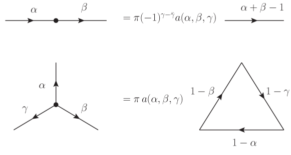
Figure 7: The chain and star– triangle relations, $\alpha+\beta+\gamma=2$.

In this Appendix we present the basic elements of the diagram technique which was used throughout the paper. The functions and kernels of operators considered in the main body of the paper are represented in the form of two-dimensional Feynman diagrams. The propagator which is shown by the arrow directed from $w$ to $z$ and index α attached to it as shown in Fig. 1 is given by the following expression

$$\frac{1}{[z-w]^{\alpha}}\equiv\frac{1}{(z-w)^{\alpha}(\bar{z}-\bar{w})^{\bar{\alpha}}}=\frac{(\bar{z}-\bar{w})^{\alpha-\bar{\alpha}}}{|z-w|^{2\alpha}}=\frac{(-1)^{\alpha-\bar{\alpha}}}{[w-z]^{\alpha}}\,,$$ (A.135)

where $\alpha-\bar{\alpha}=n_{\alpha}$ is integer. Making the Fourier transformation we define the propagator in the momentum representation

$$\int d^{2}z\frac{e^{i(pz+\bar{p}\bar{z})}}{[z]^{\alpha}}=\pi\,i^{\alpha-\bar{\alpha}}\,a(\alpha)\,\frac{1}{[p]^{1-\alpha}}\,.$$ (A.136)

Here the notation $a(\alpha)$ is introduced for the function

$$a(\alpha)=\frac{\Gamma(1-\bar{\alpha})}{\Gamma(\alpha)}\,,\quad a(\bar{\alpha})=\frac{\Gamma(1-\alpha)}{\Gamma(\bar{\alpha})}\,,\quad a(\alpha,\beta,\gamma,\ldots)=a(\alpha)a(\beta)a(\gamma)\ldots$$ (A.137)

It has the following properties

$$a(\alpha)a(1-\bar{\alpha})=1\,,\quad\frac{a(1+\alpha)}{a(\alpha)}=-\frac{1}{\alpha\bar{\alpha}}\,,\quad a(\alpha)a(1-\alpha)=(-1)^{\alpha-\bar{\alpha}}\,,\quad a(\alpha)=(-1)^{\alpha-\bar{\alpha}}a(\bar{\alpha})\,.$$

Making use of Eq. (A.136) it is easy to derive the following useful representation for the fractional derivative $[i\partial]^{\alpha}$,

$$\int d^{2}w\frac{1}{[z-w]^{\alpha}}f(w)=\pi(-i)^{\alpha-\bar{\alpha}}\,a(\alpha)\,[i\partial]^{\alpha-1}\,f(z).$$ (A.138)

The evaluation of Feynman diagrams is based on their transformation with the help of the certain ”integration rules”

• Chain relation:

  $$\int d^{2}w\frac{1}{[z_{1}-w]^{\alpha}[w-z_{2}]^{\beta}}=(-1)^{\gamma-\bar{\gamma}}a(\alpha,\beta,\gamma)\frac{1}{[z_{1}-z_{2}]^{\alpha+\beta-1}}\,,$$ (A.139)

  where $\gamma=2-\alpha-\beta,\ \bar{\gamma}=2-\bar{\alpha}-\bar{\beta}$.

• Star– triangle relation:

  $$\int d^{2}w\frac{1}{[z_{1}-w]^{\alpha}[z_{2}-w]^{\beta}[z_{3}-w]^{\gamma}}=\frac{\pi a(\alpha,\beta,\gamma)}{[z_{2}-z_{1}]^{1-\gamma}[z_{1}-z_{3}]^{1-\beta}[z_{3}-z_{2}]^{1-\alpha}}\,,$$ (A.140)

  where $\alpha+\beta+\gamma=2$ and $\bar{\alpha}+\bar{\beta}+\bar{\gamma}=2$. In an operator form star-triangle relation reads [48]

  $$[z]^{\alpha}\,[i\partial]^{\alpha+\beta}\,[z]^{\beta}=[i\partial]^{\beta}\,[z]^{\alpha+\beta}\,[i\partial]^{\alpha}\,.$$ (A.141)

• Cross relation:

  $$\frac{1}{[z_{1}-z_{2}]^{\alpha^{\prime}-\alpha}}\int d^{2}w\frac{a(\alpha^{\prime},\bar{\beta}^{\prime})}{[w-z_{1}]^{\alpha}[w-z_{2}]^{1-\alpha^{\prime}}[w-z_{3}]^{\beta}[w-z_{4}]^{1-\beta^{\prime}}}=$$

  $$=\frac{1}{[z_{3}-z_{4}]^{\beta^{\prime}-\beta}}\int d^{2}w\frac{a(\alpha,\bar{\beta})}{[w-z_{1}]^{\alpha^{\prime}}[w-z_{2}]^{1-\alpha}[w-z_{3}]^{\beta^{\prime}}[w-z_{4}]^{1-\beta}}\,,$$ (A.142)

  where $\alpha+\beta=\alpha^{\prime}+\beta^{\prime}$.

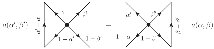
Figure 8: The cross relation, $\alpha+\beta=\alpha^{\prime}+\beta^{\prime}$.

These relations are shown in diagrammatic form in Figs. 7, 8.

Finally, we give two representations for the $\delta$ function. The first one

$$\delta^{2}(z)=\lim_{\epsilon\to 0}\frac{a(i\epsilon)}{\pi}\frac{1}{[z]^{1-i\epsilon}}=\lim_{\epsilon\to 0}\frac{i\epsilon}{\pi}\frac{1}{[z]^{1-i\epsilon}}$$ (A.143)

follows directly from Eq. (A.136) and the second relation

$$\int d^{2}w\frac{1}{[z_{1}-w]^{2-\alpha}[w-z_{2}]^{\alpha}}=\pi^{2}\,a(\alpha,2-\alpha)\,\delta^{2}(z_{1}-z_{2})\,$$ (A.144)

results from the chain relation (A.139) and (A.143).

Appendix B Proof of commutativity

The proof of the commutativity of the “transfer matrices” $\mathcal{T}_{\boldsymbol{s}_{0}}(\boldsymbol{u})$, Eq. (63bmcl) is based on the Yang-Baxter relation

$$\mathcal{R}_{\boldsymbol{s}_{0}\boldsymbol{s}_{0^{\prime}}}(\boldsymbol{u}-\boldsymbol{v})\mathbb{T}_{\boldsymbol{s}_{0}}(\boldsymbol{u})\mathbb{T}_{\boldsymbol{s}_{0^{\prime}}}(\boldsymbol{v})=\mathbb{T}_{\boldsymbol{s}_{0^{\prime}}}(\boldsymbol{v})\mathbb{T}_{\boldsymbol{s}_{0}}(\boldsymbol{u})\mathcal{R}_{\boldsymbol{s}_{0}\boldsymbol{s}_{0^{\prime}}}(\boldsymbol{u}-\boldsymbol{v})$$ (B.145)

and two special identities for the kernel of the operator $\mathcal{R}_{\boldsymbol{s}_{0}\boldsymbol{s}_{0^{\prime}}}(\boldsymbol{u}-\boldsymbol{v})$:

$$\int d^{2}w_{1}\,d^{2}w_{2}\,\mathcal{R}_{\boldsymbol{s}_{0}\boldsymbol{s}_{0^{\prime}}}(\boldsymbol{u})(z_{1},z_{2}|w_{1},w_{2})=C(u,s_{0},s_{0^{\prime}})\,,$$ (B.146)

$$\lim_{z_{1},z_{2}\to z}\mathcal{R}_{\boldsymbol{s}_{0}\boldsymbol{s}_{0^{\prime}}}(\boldsymbol{u})(z_{1},z_{2}|w_{1},w_{2})=C(u,s_{0},s_{0^{\prime}})\,\delta^{2}(z-w_{1})\,\delta^{2}(z-w_{2})\,,$$ (B.147)

where $C(u,s_{0},s_{0}^{\prime})$ is some coefficient. The kernels on the l.h.s and r.h.s. of Eq. (B.145) depend on the variables $(z_{k},w_{k})$, $k=1,\ldots,N$ in the quantum space and the variables $z_{0},z_{0^{\prime}},w_{0},w_{0^{\prime}}$ associated with the two auxiliary spaces. Sending $z_{0},z_{0^{\prime}}\to 0$ and integrating over $w_{0},w_{0^{\prime}}$ in both parts of Eq. (B.145) with the help of Eqs. (B.146), (B.147) one immediately gets Eq. (63bmcl).

The identities (B.146), (B.147) follow from the analogous identities for the factorized operators $\mathcal{R}_{12}^{(k=1,2)}$, see Eq. (27):

$$\int d^{2}w_{1}\,d^{2}w_{2}\,\mathcal{R}_{12}^{(k)}(u,v)(z_{1},z_{2}|w_{1},w_{2})=A^{(k)}(u,v)\,,$$ (B.148)

$$\lim_{z_{1}\to z,z_{2}\to z}\mathcal{R}_{12}^{(k)}(u,v)(z_{1},z_{2}|w_{1},w_{2})=A^{(k)}(u)\,\delta^{2}(z-w_{1})\,\delta^{2}(z-w_{2})\,,$$ (B.149)

where $A^{(2)}(u,v)=A^{(1)}(v,u)$ and

$$A^{(1)}(u,v)=\pi\,(-1)^{i(v-\bar{v})}\,a(iv,1-iu,1+iu-iv).$$ (B.150)

To derive Eqs. (B.146) or (B.148) it is sufficient to use the chain relation (A.139). In order to obtain (B.148) one has to represent the kernel in the form of the star diagram using the star-triangle relation (A.140) then send $z_{1}\to z_{2}$ and use the chain integration rule (A.144). Eq. (B.147) follows from Eqs. (B.149) and (28).

References

References

[1]
H. Bethe,
“On the theory of metals. 1. Eigenvalues and eigenfunctions for the linear atomic chain,”
Z. Phys. 71 (1931) 205.
[2]
R. J. Baxter, Exactly Solved Models in Statistical
Mechanics, Academic Press, London, 1982.
[3]
L. D. Faddeev,
“How algebraic Bethe ansatz works for integrable model”,
In: Quantum Symmetries/Symetries Quantiques,
Proc.Les-Houches summer school, LXIV.
Eds. A.Connes,K.Kawedzki, J.Zinn-Justin. North-Holland, 1998, 149-211,
hep-th/9605187.
[4]
L. D. Faddeev, E. K. Sklyanin and L. A. Takhtajan,
“The Quantum Inverse Problem Method. 1,”
Theor. Math. Phys. 40 (1980) 688
[Teor. Mat. Fiz. 40 (1979) 194].
[5]
L. A. Takhtajan and L. D. Faddeev,
“The Quantum method of the inverse problem and the Heisenberg XYZ model”,
Russ. Math. Surveys 34 (1979) 11
[Usp. Mat. Nauk 34 (1979) 13].
[6]
P. P. Kulish and E. K. Sklyanin,
“Quantum Spectral Transform Method. Recent Developments”,
Lect. Notes Phys. 151 (1982) 61.
[7]
E. K. Sklyanin,
“Quantum Inverse Scattering Method”, in
Quantum Groups and Quantum Integrable Systems, (Nankai
lectures), ed. Mo-Lin Ge, pp. 63-97, World Scientific Publ.,
Singapore 1992, [hep-th/9211111]
[8]
M. C. Gutzwiller,
“The Quantum Mechanical Toda Lattice. II,”
Annals Phys. 133 (1981) 304.
[9]
E. K. Sklyanin,
Lect. Notes Phys. 226 (1985) 196.
[10]
M. Gaudin and V. Pasquier,
“The periodic Toda chain and a matrix generalization of the bessel function’s recursion relations,”
J. Phys. A 25 (1992) 5243.
[11]
S. Kharchev and D. Lebedev,
“Integral representation for the eigenfunctions of quantum periodic Toda chain,”
Lett. Math. Phys. 50 (1999) 53.
[12]
V. V. Bazhanov, S. L. Lukyanov and A. B. Zamolodchikov,
“Integrable structure of conformal field theory, quantum KdV theory and thermodynamic Bethe ansatz,”
Commun. Math. Phys. 177 (1996) 381.
[13]
V. V. Bazhanov, S. L. Lukyanov and A. B. Zamolodchikov,
“Integrable structure of conformal field theory. 2. Q operator and DDV equation,”
Commun. Math. Phys. 190 (1997) 247.
[14]
R. J. Baxter,
“Partition function of the eight vertex lattice model,”
Annals Phys. 70 (1972) 193
[Annals Phys. 281 (2000) 187].
[15]
E. K. Sklyanin,
“Separation of variables - new trends,”
Prog. Theor. Phys. Suppl. 118 (1995) 35.
[16]
L. N. Lipatov,
“Small x physics in perturbative QCD,”
Phys. Rept. 286 (1997) 131.
[17]
L. N. Lipatov,
“High-energy asymptotics of multicolor QCD and two-dimensional conformal field theories,”
Phys. Lett. B 309 (1993) 394.
[18]
L. N. Lipatov,
“High-energy asymptotics of multicolor QCD and exactly solvable lattice models.”
JETP Lett. 59 (1994) 596-599; Pisma Zh.Eksp.Teor.Fiz. 59 (1994) 571-574
[19]
L. D. Faddeev and G. P. Korchemsky,
“High-energy QCD as a completely integrable model,”
Phys. Lett. B 342 (1995) 311.
[20]
H. J. De Vega and L. N. Lipatov,
“Interaction of reggeized gluons in the Baxter-Sklyanin representation,”
Phys. Rev. D 64 (2001) 114019.
[21]
H. J. de Vega and L. N. Lipatov,
“Exact resolution of the Baxter equation for reggeized gluon interactions,”
Phys. Rev. D 66 (2002) 074013.
[22]
S. E. Derkachov, G. P. Korchemsky and A. N. Manashov,
“Noncompact Heisenberg spin magnets from high-energy QCD: 1. Baxter Q operator and separation of variables,”
Nucl. Phys. B 617 (2001) 375.
[23]
S. E. Derkachov, G. P. Korchemsky, J. Kotanski and A. N. Manashov,
“Noncompact Heisenberg spin magnets from high-energy QCD. 2. Quantization conditions and energy spectrum,”
Nucl. Phys. B 645 (2002) 237.
[24]
L. N. Lipatov,
“Integrability of scattering amplitudes in N=4 SUSY,”
J. Phys. A 42 (2009) 304020.
[25]
J. Bartels, L. N. Lipatov and A. Prygarin,
“Integrable spin chains and scattering amplitudes,”
J. Phys. A 44 (2011) 454013.
[26]
J.M. Maillet and J. S anchez de Santos,
“Drinfel d twists and algebraic Bethe ansatz,”
Amer. Math. Soc. Transl. 201 (2000), 137 178.
[27]
V. Terras,
“Drinfeld twists and
Functional Bethe Ansatz,”
Lett. Math. Phys. 48 (1999) 263.
[28]
S. E. Derkachov,
Factorization of the R-matrix. I.,
math/0503396 [math-qa].
[29]
S. E. Derkachov and A. N. Manashov,
General solution of the Yang-Baxter equation
with symmetry group SL(n,C),
St. Petersburg Math. J. 21, 513 (2010)
[Alg. Anal. 21N4, 1 (2009)].
[30]
S. Kharchev and D. Lebedev,
“Integral representations for the eigenfunctions of quantum open and periodic Toda chains from QISM formalism,”
J. Phys. A 34 (2001) 2247.
[31]
A. V. Silantyev, ”Transition function for the Toda chain.”,
Theor. Math. Phys. 150 (2007), 315–331.
[32]
K. K. Kozlowski,
”Unitarity of the SoV transform for the Toda chain”,
math.ph:1306.4967.
[33]
S. E. Derkachov, G. P. Korchemsky and A. N. Manashov,
“Separation of variables for the quantum SL(2,R) spin chain,”
JHEP 0307 (2003) 047.
[34]
S. E. Derkachov, G. P. Korchemsky and A. N. Manashov,
“Baxter Q operator and separation of variables for the open SL(2,R) spin chain,”
JHEP 0310 (2003) 053.
[35]
G. Niccoli,
“Form factors and complete spectrum of XXX antiperiodic higher spin chains by quantum separation of variables,”
J. Math. Phys. 54 (2013) 053516.
[36]
A. G. Bytsko and J. Teschner,
“Quantization of models with non-compact quantum group symmetry:
Modular XXZ magnet and lattice sinh-Gordon model”,
J. Phys. A 39 (2006) 12927.
[37]
G. Niccoli,
“Completeness of Bethe Ansatz by Sklyanin SOV for Cyclic Representations of Integrable Quantum Models,”
JHEP 1103 (2011) 123.
[38]
G. Niccoli,
“Antiperiodic spin-1/2 XXZ quantum chains by separation of variables: Complete spectrum and form factors,”
Nucl. Phys. B 870 (2013) 397.
[39]
S. Faldella, N. Kitanine and G. Niccoli,
“Complete spectrum and scalar products for the open spin-1/2 XXZ quantum chains with non-diagonal boundary terms,”
arXiv:1307.3960 [math-ph].
[40]
I. M. Gelfand, M. I. Graev and N. Ya. Vilenkin, Generalized functions, Vol. 5, Academic
Press, 1966.
[41]
P. P. Kulish, N. Y. .Reshetikhin and E. K. Sklyanin,
“Yang-Baxter Equation and Representation Theory. 1.,”
Lett. Math. Phys. 5 (1981) 393.
[42]
S. E. Derkachov and A. N. Manashov,
“R-matrix and baxter Q-operators for the noncompact SL(N,C) invariant spin chain,”
SIGMA 2 (2006) 084.
[43]
F. A. Smirnov,
“Form-factors in completely integrable models of quantum field theory,”
Adv. Ser. Math. Phys. 14 (1992) 1.
[44]
N. Kitanine, J.M. Maillet, and V. Terras,
“Form Factors of the XXZ Heisenberg
spin-1/2 ?nite chain,”
Nucl. Phys. B554 (1999), 647 678.
[45]
S. E. Derkachov,
“Baxter’s Q-operator for the homogeneous XXX spin chain,”
J. Phys. A 32 (1999) 5299.
[46]
L. N. Lipatov,
“Duality symmetry of Reggeon interactions in multicolor QCD,”
Nucl. Phys. B 548 (1999) 328.
[47]
J. Bartels, L. N. Lipatov and A. Sabio Vera,
“N=4 supersymmetric Yang Mills scattering amplitudes at high energies: The Regge cut contribution,”
Eur. Phys. J. C 65 (2010) 587.
[48]
A. P. Isaev,
“Multiloop Feynman integrals and conformal quantum mechanics,”
Nucl. Phys. B 662 (2003) 461.
[49]
V. O. Tarasov,
“Cyclic monodromy matrices for the R matrix of the six vertex model and the chiral
Potts model with fixed spin boundary conditions,”
Int. J. Mod. Phys. A 7S1B, 963 (1992).