Cyclopermutohedron
(To Nilolai Dolbilin, who loves polytopes)

Abstract.

It is known that the $k$-faces of the permutohedron $\Pi_{n}$ can be labeled by (all possible) linearly ordered partitions of the set $[n]=\{1,...,n\}$ into $(n-k)$ non-empty parts. The incidence relation corresponds to the refinement: a face $F$ contains a face $F^{\prime}$ whenever the label of $F^{\prime}$ refines the label of $F$.

In the paper we consider the cell complex ${CP}_{n+1}$ defined in analogous way, replacing linear ordering by cyclic ordering. Namely, $k$-cells of the complex ${CP}_{n+1}$ are labeled by (all possible) cyclically ordered partitions of the set $[n+1]=\{1,...,n,n+1\}$ into $(n+1-k)$ non-empty parts, where $(n+1-k)>2$. The incidence relation in ${CP}_{n+1}$ again corresponds to the refinement: a cell $F$ contains a cell $F^{\prime}$ whenever the label of $F^{\prime}$ refines the label of $F$.

The complex ${CP}_{n+1}$ cannot be represented by a convex polytope, since it is not a combinatorial sphere (not even a combinatorial manifold). However, it can be represented by some virtual polytope (that is, Minkowski difference of two convex polytopes) which we call ”cyclopermutohedron” $\mathcal{CP}_{n+1}$. It is defined explicitly, as a weighted Minkowski sum of line segments. Informally, the cyclopermutohedron can be viewed as ”permutohedron with diagonals”. One of the motivations is that the cyclopermutohedron is a ”universal” polytope for moduli spaces of polygonal linkages.

1. Preliminaries

Among all famous polytopes with combinatorial backgrounds, the standard permutohedron $\Pi_{n}$ is the oldest and probably the most important one. It is defined (see [11]) as the convex hull of all points in $\mathbb{R}^{n}$ that are obtained by permuting the coordinates of the point $(1,2,...,n)$. It has the following properties:

1. $\Pi_{n}$ is an $(n-1)$-dimensional polytope.

2. The $k$-faces of $\Pi_{n}$ are labeled by ordered partitions of the set
   $[n]=\{1,2,...,n\}$ into $(n-k)$ non-empty parts.

3. In particular, the vertices are labeled by the elements of the symmetry group $S_{n}$. For each vertex, the label is the inverse permutation of the coordinates of the vertex. Two vertices are joined by an edge whenever their labels differ by a permutation of two neighbor entries.

4. A face $F$ of $\Pi_{n}$ is contained in a face $F^{\prime}$ iff the label of $F$ is a refinement of the label of $F^{\prime}$.

   Here and in the sequel, we mean the order-preserving refinement. For instance, $(\{1,3\},\{5,6\},\{4\},\{2\})$ refines $(\{1,3\},\{5,6\},\{2,4\})$, but does not refine $(\{1,3\},\{2,4\},\{5,6\})$.

5. Each face of $\Pi_{n}$ equals the Cartesian product of standard permutohedra of smaller dimensions.

6. The permutohedron is a zonotope, that is, Minkowski sum of line segments.

7. The permutohedra $\Pi_{1}$, $\Pi_{2}$, and $\Pi_{3}$ are a one-point polytope, a segment, and a regular hexagon respectively. The permutohedron $\Pi_{4}$ is depicted in Figure 1.

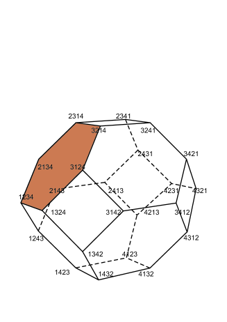
Figure 1. Permutahedron $\Pi_{4}$ with labels on the vertices. The shadowed face is labeled by $(\{1,2,3\}\{4\})$.

Historically, the permutohedron was followed by associahedron, cyclohedron (see [11]), permutoassociahedron (see [4]), and more advanced polytopes appearing first as combinatorially described cell complexes: secondary polytope [2], generalized associahedra [1]. The complexes luckily appeared to be combinatorial spheres, and moreover, representable by convex polytopes. A wider framework includes graph-associahedra, nestohedra [10], and other recently constructed polytopes.

In the paper, we proceed in the same manner: we first describe a cell complex ${CP}_{n+1}$, and then show that it can be represented by a virtual polytope, i.e., by Minkowski difference of two convex polytopes. We guess that virtual polytopes (as the tightest algebraic generalization of convex polytopes, originally introduced in [5]) provide us a reasonable framework for this particular complex.

The combinatorics of the complex ${CP}_{n+1}$ almost literally repeats the combinatorics of permutohedron with one essential difference: linear ordering is replaced by cyclic ordering. Thus defined, complex ${CP}_{n+1}$ cannot be represented by a convex polytope, since it is not a combinatorial sphere (not even a combinatorial manifold). However, it can be represented by a virtual polytope which we call cyclopermutohedron $\mathcal{CP}_{n+1}$. It is defined explicitly, as a weighted Minkowski sum of line segments. The word ”weighted” means that some of the summands are negatively weighted, that is, we take not only Minkowski sum, but also Minkowski difference.

In an oversimplified way, the cyclopermutohedron $\mathcal{CP}_{n+1}$ can be visualized as the permutohedron $\Pi_{n}$ ”with diagonals”. This means that all the proper faces of $\Pi_{n}$ are also faces of $\mathcal{CP}_{n+1}$. However, $\mathcal{CP}_{n+1}$ has some extra faces in comparison with $\Pi_{n}$. The latter look like ”diagonal” faces, see Figure 5.

The idea to replace linear ordering by cyclic ordering in the framework of ”famous polytopes” is not new: replacing linear ordering in the combinatorics of associahedron yields the cyclohedron.

Although the cyclopermutohedron seems to be interesting for its own sake, we were initially motivated by yet another application: the cyclopermutohedron is a ”universal” polytope for moduli spaces of polygonal linkages. That is, for any length assignment of a planar flexible polygon with $(n+1)$ edges, its moduli space admits a natural cell structure which embeds in the (cell structure of) the cyclopermutohedron $\mathcal{CP}_{n+1}$.

The paper is organized as follows. Section 2 describes a regular cell complex which we wish to realize as the face lattice of the cyclopermutohedron. Section 3 contains the construction, the main statements (Proposition 2 and Theorem 1), and low dimensional examples of the cyclopermutohedra. The main theorem (Theorem 1) establishes combinatorial equivalence of the cyclopermutohedron and the cell complex. Next, Section 4 explains the relationship with the moduli space of a planar polygonal linkage. The proofs of Theorem 1 and Proposition 2 are in Section 5. To make the paper self-contained, we put all necessary information on virtual polytopes in Section 6.

2. Cyclopermutohedron: the desired combinatorics

By a regular cell complex we mean a finite cell complex which can be constructed inductively by defining its skeleta. The $0$-skeleton is a finite set of points endowed with discrete topology. Once the $(k-1)$-skeleton is constructed, we attach a collection of closed $k$-dimensional balls $C_{i}$, called closed cells. For each of $C_{i}$, the attaching map is a homeomorphism between $\partial C_{i}$ and a sphere homeomorphic subcomplex of the $(k-1)$-skeleton.

By construction, the boundary of each closed cell has the induced structure of a regular cell complex.

To define a regular cell complex, it suffices to list all the closed cells of the complex together with the incidence relations. Following this rule, for a fixed number $n>2$, we define the regular cell complex ${CP}_{n+1}$ as follows.

• For $k=0,...,n-2$, the $k$-dimensional cells ($k$-cells, for short) of the complex ${CP}_{n+1}$ are labeled by (all possible) cyclically ordered partitions of the set $[n+1]=\{1,...,n+1\}$ into $(n-k+1)$ non-empty parts.

• A (closed) cell $F$ contains a cell $F^{\prime}$ whenever the label of $F^{\prime}$ refines the label of $F$. Here we mean orientation preserving refinement.

In particular, this means that the vertices of the complex ${CP}_{n+1}$ are labeled by cyclic orderings on the set $[n+1]$. Two vertices are joined by an edge whenever their labels differ on a permutation of two neighbor entries.

Let us first give an example, next agree how we depict the labels, and then prove the correctness of the above construction.

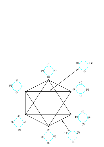
Figure 2. The complex ${CP}_{4}$.

Example 1.

For $n=3$, the complex ${CP}_{n+1}={CP}_{4}$ consists of six vertices and twelve edges. In the figure 2, all the vertices and two of the edges are labeled.

A convention about presenting the labels

Let us agree that instead of saying ”the cell of the complex labeled by $\lambda$” we say for short ”the cell $\lambda$”.

We shall write a cyclically ordered partition $\lambda$ in the following ways:

1. Sometimes we depict $\lambda$ as a counterclockwise oriented circle with subsets placed on the circle, as in Figure 2.

2. Alternatively, we cut $\lambda$ at any place and get a string of sets $(I_{1},I_{2},...,I_{k})$. We keep in mind that

   $$(I_{1},I_{2},...,I_{k})=cycl(I_{1},I_{2},...,I_{k})=(I_{k},I_{1},I_{2},...,I_{k-1})=$$

   $$=cycl^{2}(I_{1},I_{2},...,I_{k})=(I_{k-1},I_{k},I_{1},I_{2},...,I_{k-3},I_{k-2}),\hbox{ etc}.$$

3. For the vertices of ${CP}_{n+1}$, we use one more type of reduction. Given a label $\lambda$ of a vertex (that is, a cyclic ordering on $[n+1]$), we write its label as the linear ordering on $[n]$, which is obtained from $\lambda$ by cutting through the entry $(n+1)$ and removing the entry $(n+1)$ from the string. The obtained label we denote by $\overline{\lambda}$.

   For instance, the label

   $$\lambda=(\{3\},\{4\},\{1\},\{5\},\{6\},\{2\})$$

   yields

   $$\overline{\lambda}=(2,3,4,1,5).$$

   Conversely, given a linear ordering $\overline{\lambda}$ on the set $[n]$, we cook a cyclically ordered partitions of the set $[n+1]$ into $(n+1)$ singletons by adding at the end the set $\{n+1\}$ and closing the string in a cycle.

   For instance, $(3,2,1)\in S_{3}$ yields $(\{3\},\{2\},\{1\}),$ and then the cyclically ordered partition

   $$\begin{array}[]{ccc}&\{3\}&\\ \{2\}&&\{4\}.\\ &\{1\}&\end{array}$$

Proposition 1.

For each $n\geq 3$, the complex ${CP}_{n+1}$ is defined correctly and uniquely.

Proof. We construct the complex inductively. The $0$-skeleton is obviously well-defined. Assume that we have already the $k$-skeleton and that we wish to attach a $(k+1)$-cell $C$ labeled by some cyclically ordered partition

$$(I_{1},I_{2},...,I_{n-k})=(I_{2},I_{3},...,I_{n-k},I_{1})=(I_{3},I_{4},...,I_{1},I_{2})=....$$

All the cells of the $k$-skeleton that should be incident to $C$ form a subcomplex of the $k$-skeleton which is combinatorially isomorphic to the boundary complex of the Cartesian product of permutohedra

$$\partial(\Pi_{n_{1}}\times...\times\Pi_{n_{n-k}}),$$

where $n_{i}=|I_{i}|$. Obviously, it is a $k$-dimensional sphere, and there is a unique way to attach the boundary $\partial C$ to the sphere.∎

Corollary 1.

Each closed cell of the complex ${CP}_{n+1}$ is combinatorially equivalent to a Cartesian product of permutohedra. ∎

Lemma 1.

Let $\lambda=(I_{1},I_{2},...,I_{k})$ be the label of some cell of the complex ${CP}_{n+1}$. We assume that the entry $(n+1)$ belongs to the set $I_{k}$.

The (labels of the) vertices of the cell $\lambda$ can be retrieved via the following algorithm:

1. Take the string $\lambda=(I_{1},I_{2},...,I_{k})$ and remove the entry $n+1$ from $I_{k}$.

2. Take all possible orderings inside each of the sets $I_{j},\ j=1,2,...,k,$ and list all the resulting strings. We get some set $V(\lambda)$.

3. Apply cyclic permutations $cycl^{0},cycl^{1},cycl^{2},...,cycl^{|I_{k}|-1}$ to all the elements of $V(\lambda)$. We get

   $$V_{0}(\lambda)=V(\lambda),\ V_{1}(\lambda):=cycl^{1}V(\lambda),...,V_{|I_{k}|-1}(\lambda):=cycl^{|I_{k}|-1}V(\lambda).$$

4. The vertex set of the cell $\lambda$ is the union of the sets:

   $$Vert(\lambda)=V_{0}\bigcup V_{1}\bigcup V_{2}\bigcup...\bigcup V_{|I_{k}|-1}.\qed$$

Example 2.

For $\lambda=(\{1,2\},\{3\},\{4,5,6\})$, we have

$$Vert(\lambda)=$$

$$\{(1,2,3,4,5),(1,2,3,5,4),\ (2,1,3,5,4),\ (2,1,3,4,5),$$

$$(5,1,2,3,4),\ (4,1,2,3,5),\ (4,2,1,3,5),\ (5,2,1,3,4),$$

$$(4,5,1,2,3,),\ (5,4,1,2,3),\ (5,4,2,1,3),\ (4,5,2,1,3,)\}.\qed$$

To give a reader more intuition, we complete the section by yet another example.

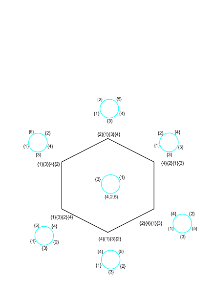
Figure 3. The $2$-face of the complex $CP_{5}$ labeled by $(\{1\}\{3\}\{4,2,5\})$

Example 3.

For $n=4$, Figure 3 presents a hexagonal $2$-face of the complex $CP_{5}$ and all the vertices of the face.

3. Cyclopermutohedron: realization as a virtual polytope

Assuming that $\{e_{i}\}$ are standard basic vectors in $\mathbb{R}^{n}$, define the points

$$\begin{array}[]{ccccccccc}R_{i}=\sum_{j=1}^{n}(e_{j}-e_{i})=(-1,&...&-1,&n-1,&-1,&...&-1,&-1,&-1,)\in\mathbb{R}^{n},\\ &&&\ i&&&&&\end{array}$$

and the following two families of line segments:

$$q_{ij}=\left[e_{i},e_{j}\right],\ \ \ i<j$$

and

$$r_{i}=\left[0,R_{i}\right].$$

We also need the point $S=\left(1,1,...,1\right)\in\mathbb{R}^{n}$.

Definition 1.

The cyclopermutohedron is a virtual polytope defined as the weighted Minkowski sum of line segments:

$$\mathcal{CP}_{n+1}:=\sum_{i<j}q_{ij}+S-\sum_{i=1}^{n}r_{i}.$$

Clearly, $\mathcal{CP}_{n+1}$ lies in the hyperplane

$$x_{1}+...+x_{n}=\frac{n(n+1)}{2},$$

so its actual dimension is $(n-1)$.

Remark 1.

The Minkowski sum

$$\sum_{i<j}q_{ij}+S$$

is known to be equal to the standard permutohedron $\Pi_{n}$ (see [11]). Therefore we can write

$$\mathcal{CP}_{n+1}=\Pi_{n}-\sum_{i=1}^{n}r_{i}.$$

Remark 2.

The symmetric group $S_{n}$ acts on the $\mathbb{R}^{n}$ by permuting the coordinates. The action preserves the sets $\{q_{i,j}\}$ and $\{r_{i}\}$, so both permutohedron and cyclopermutohedron are invariant under the action. We shall refer to this property as the symmerty property of the polytopes.

A curios and crucial feature of the cyclopermutohedron is the following:

Proposition 2.

The set of vertices of $\mathcal{CP}_{n+1}$ equals the set of vertices of the standard permutohedron $\Pi_{n}$:

$$Vert(\mathcal{CP}_{n+1})=Vert(\Pi_{n}).\qed$$

The proposition allows us to label the vertices of the cyclopermutohedron by the labels borrowed from the permutohedron.

More detailed, each vertex $v$ of $\mathcal{CP}_{n+1}$ is a vertex of $\Pi_{n}$, and therefore, its coordinates is some permutation on $[n]$. We label the vertex $v$ by the inverse permutation. For instance, the vertex with coordinates $(4,1,5,3,2)$ is labeled by $\lambda=(2,5,4,1,3)$.

Next, remind that each label yields automatically a cyclic ordering on the set $[n+1]$ by adding to $\lambda$ the entry $(n+1)$ at the end and closing the label in the circle.

Therefore we have:

Corollary 2.

The vertices of $\mathcal{CP}_{n+1}$ are canonically labeled by (all possible) cyclic orderings on the set $[n+1]$.

Definition 2.

We define a bijection

$$\varphi:Vert(CP_{n+1})\rightarrow Vert(\mathcal{CP}_{n+1})$$

between the vertex sets of the cell complex $CP_{n}$ and the cyclopermutohedron. Given a vertex $v\in Vert(CP_{n+1})$ labeled by $\lambda$, the bijection $\varphi$ maps it to the vertex of the $\mathcal{CP}_{n}$ labeled by $\overline{\lambda}$. By construction, it coincides with the vertex of $\Pi_{n}$ labeled by $\overline{\lambda}$.

Theorem 1.

The bijection $\varphi$ extends to a combinatorial isomorphism between the complex $CP_{n+1}$ and the cyclopermutohedron $\mathcal{CP}_{n+1}$.

More precisely, the following holds:

1. A subset $V\subset Vert(CP_{n+1})$ is the vertex set of some cell of the complex $CP_{n+1}$ if and only if $\varphi(V)$ is the vertex set of some face of $\mathcal{CP}_{n+1}$.

2. The $k$-faces of $\mathcal{CP}_{n+1}$ can be labeled by (all possible) cyclically ordered partitions of the set $[n+1]$ into $(n-k+1)$ non-empty parts.

3. With this labeling, a face $F^{\prime}$ is a face of a face $F$ if and only if the label of $F^{\prime}$ refines the label of $F$.

∎

Example 4.

$\mathcal{CP}_{4}$ is a two-dimensional virtual polytope, however, the definition puts in in $\mathbb{R}^{3}$. Figure 4, left depicts the virtual polytope

$$\sum_{1\geq i>j\geq 3}q_{ij}-\sum_{i=1}^{3}r_{i}.$$

After the parallel translation by $S=(1,1,1)$, we get the cyclopermutohedron $\mathcal{CP}_{4}$ (right). (A more detailed explanation of how to compute Minkowski difference in the plane one finds in Section 6). In the figure, we indicate the coordinates of the vertices. After replacing coordinates by labels, we arrive exactly at the complex $CP_{4}$ (compare with Figure 2).

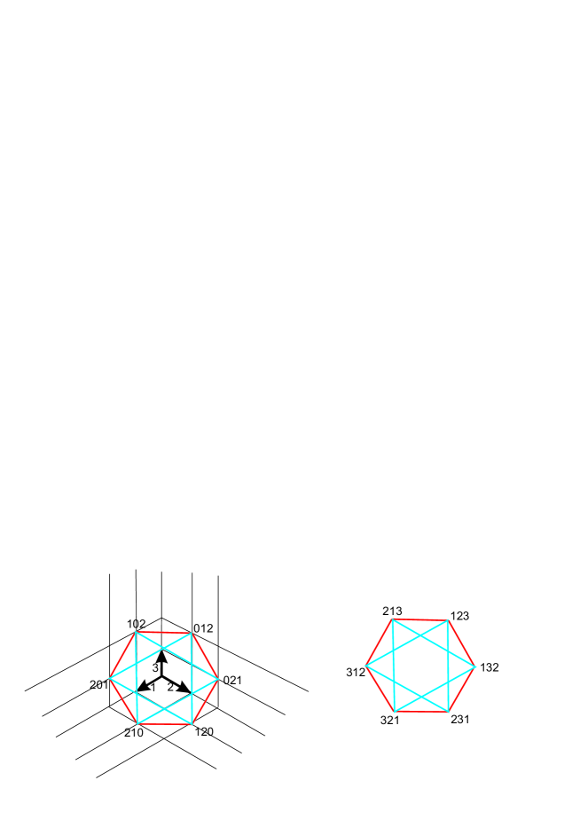
Figure 4. Basis vectors in $\mathbb{R}^{3}$, the polytope $\sum_{i<j}q_{ij}-\sum_{i=1}^{3}r_{i}$ (left), and the cyclopermutohedron $\mathcal{CP}_{4}$ with coordinates of the vertices (right).

Example 5.

The cyclopermutogedron $\mathcal{CP}_{5}$ is a $3$-dimensional virtual polytope. Here is the complete list of its faces (see also Figure 5).

1. By Proposition 2, the vertices of $\mathcal{CP}_{5}$ are the vertices of the standard permutohedron $\Pi_{4}$.

2. The edges are of two types: those coinciding with the edges of the standard permutohedron $\Pi_{4}$, and diagonal edges equal to the parallel translates of the segments $r_{i}$. The labels of the endpoints of a diagonal edge differ by a cyclic permutation $cycl$.

   For instance, the vertices $(2,1,4,3)$ and $(1,4,3,2)$ share a diagonal edge which is a parallel translate of $r_{2}=[0,(-1,3,-1,-1)]$.

3. The $2$-faces fall into four categories (see Figure 5):

   1. Virtual hexagons of type $(q_{ij}-r_{i}-r_{j})$. These are combinatorial permutohedra $\Pi_{3}$.

   2. Convex quadrilaterals, faces of the standard permutohedron $\Pi_{4}$.

   3. Quadrilaterals of type $q_{ij}\times(-r_{k})$, and

   4. Convex hexagons, faces of the standard permutohedron $\Pi_{4}$.

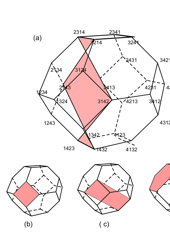
Figure 5. There are four types of $2$-faces of the cyclopermutohedron $\mathcal{CP}_{5}$. We depict here representatives of all the types. Their labels are: (a) $(\{1\}\{4\}\{2,3,5\})$, (b) $(\{1,3\}\{4,2\}\{5\})$,
(c) $(\{1,3\}\{2\}\{4,5\})$, (d) $(\{1,2,3\}\{4\}\{5\})$.

4. Cyclopermutohedron is the universal polytope for the moduli spaces of planar polygonal linkages

A polygonal $n$-linkage is a sequence of positive numbers $L=(l_{1},\dots,l_{n})$. It should be interpreted as a collection of rigid bars of lengths $l_{i}$ joined consecutively in a chain by revolving joints.

We assume that $L$ satisfies the triangle inequality.

A configuration of $L$ in the Euclidean plane $\mathbb{R}^{2}$ is a sequence of points $R=(p_{1},\dots,p_{n}),\ p_{i}\in\mathbb{R}^{2}$ with $l_{i}=|p_{i},p_{i+1}|$, and $l_{n}=|p_{n},p_{1}|$.

The set $M(L)$ of all configurations modulo orientation preserving isometries of $\mathbb{R}^{2}$ is the moduli space, or the configuration space of the linkage $L$.

We assume that no configuration of $L$ fits a straight line. This assumption implies that the moduli space $M(L)$ is a closed $(n-3)$-dimensional manifold.

Definition 3.

A partition of the set $\{l_{1},\dots,l_{n}\}$ is called admissible if the total length of any part does not exceed the total length of the rest.

In the terminology of paper [3], all parts of an admissible partition are short sequences.

Instead of partitions of $\{l_{1},\dots,l_{n}\}$ we shall speak of partitions of the set $[n]$, keeping in mind the lengths $l_{i}$.

It is proven (see [9]) that the moduli space $M(L)$ admits a structure of a regular cell complex (denoted by $CWM^{*}(L)$) whose description reads as follows.

1. The $k$-cell of the complex are labeled by (all possible) admissible cyclically ordered partition of $[n]$ into $(n-k)$ non-empty subsets. Given a cell $C$, its label is denoted by $\lambda(C)$.

2. A closed cell $C$ belongs to the boundary of another closed cell $C^{\prime}$ whenever the label $\lambda(C^{\prime})$ is finer than the label $\lambda(C)$.

In other words, the moduli space $M(L)$ is patched of the admissibly labeled cells of the complex $CP_{n}$.

An immediate consequence of the construction is the following theorem:

Theorem 2.

For any $n$-linkage $L$, the cell complex $CWM^{*}(L)$ embeds as a subcomplex in the face lattice of the cyclopermutohedron $\mathcal{CP}_{n}$.∎

5. Proofs

Definition 7 says that given a virtual polytope $K$, its faces are associated to non-zero vectors $\xi$. Thus, to list all the faces of the cyclopermutohedron, we need to compute the face $\mathcal{CP}_{n+1}^{\xi}$ for each $\xi$.

So we fix a non-zero vector $\xi=(x_{1},x_{2},...,x_{n})$, assuming by symmetry that

$$x_{1}\geq x_{2}\geq...\geq x_{n}.$$

Next, we assume that the values $x_{i}$ appear in $m$ clusters of equal entries, that is,

$$x_{1}=x_{2}=...=x_{i_{1}}>x_{i_{1}+1}=x_{i_{1}+2}=...=x_{i_{2}}>x_{i_{2}+1}=x_{i_{2}+2}=...\hbox{ etc.}$$

Denote the clusters by $U_{p}$ , and denote their lengths by $d_{p}=i_{p+1}-i_{p}$:

$$U_{1}=\{1,2,...,i_{1}\},\ U_{2}=\{i_{1}+1,i_{1}+2,...,i_{2}\},\hbox{ etc.}$$

We say that a vector $\xi$ is diagonal-free if $\xi$ is orthogonal to none of $r_{i}$. Otherwise we call $\xi$ a diagonal vector.

We first make two elementary observations:

Lemma 2.

Assume that $\xi$ is a diagonal vector, which means that $\xi$ is orthogonal to some $r_{j}$. Then $\xi$ is orthogonal to $r_{i}$ if and only if the indices $j$ and $i$ belong to one and the same cluster.∎

Lemma 3.

If $\eta$ is a small perturbation of $\xi$, then the cluster scheme related to $\eta$ refines the cluster scheme related to $\xi$. Moreover, given $\xi$, a suitable choice of a small perturbation $\eta$, one gets any prescribed refinement. ∎

Since for virtual polytopes, ”face of the sum equals sum of the faces” (see Proposition 4), we have:

$$\mathcal{CP}_{n+1}^{\xi}=\left(\sum_{i<j}q_{ij}+S-\sum_{i=1}^{n}r_{i}\right)^{\xi}=\sum_{i<j}q^{\xi}_{ij}+S+\sum_{i=1}^{n}(-r_{i})^{\xi}.$$

So we first compute the faces of the summands. The latter are either points, or (either convex or inverse to convex) line segments.

Faces of the summands

Lemma 4.

The face of the line segment $q_{ij}$ is either its vertex $e_{i}$, or the entire segment:

$$q_{ij}^{\xi}=\left\{\begin{array}[]{ll}e_{i},&\hbox{ if $i$ and $j$ belong to different clusters };\\ q_{ij},&\hbox{ if $i$ and $j$ belong to one and the same cluster.\qed}\par\end{array}\right.$$

Lemma 5.

If $\xi$ is diagonal-free, we have:

1. Let $k(\xi)=k\in\mathbb{N}$ be such that

   $$x_{k}>\frac{x_{1}+...+x_{n}}{n}>x_{k+1}.$$

   Then the face of the line segment $r_{i}$ is the point:

   $$r_{i}^{\xi}=\left\{\begin{array}[]{ll}R_{i},&\hbox{ if index }i\hbox{ preceeds }U_{k},\hbox{ that is, }i<i_{k-1}+1;\\ 0,&\hbox{ otherwise.}\end{array}\right.$$

2. By Proposition 4, for the Minkowski inverse $-r_{i}$, we have

   $$(-r_{i})^{\xi}=\left\{\begin{array}[]{ll}-R_{i},&\hbox{ if index }i\hbox{ preceeds }U_{k},\hbox{ that is, }i<i_{k-1}+1;\\ 0,&\hbox{ otherwise.\qed}\end{array}\right.$$

Lemma 6.

If $\xi$ is a diagonal vector, then there is a uniquely defined cluster $U_{k}$ such that

$$\forall i\in U_{k},\ \ \ x_{i}=\frac{x_{1}+...+x_{n}}{n}.$$

Then we have:

$$r_{i}^{\xi}=\left\{\begin{array}[]{lll}r_{i},&\hbox{ if }i\in U_{k};\\ R_{i},&\hbox{ if index }i\hbox{ preceeds }U_{k},\hbox{ that is, }i<i_{k-1}+1;\\ 0,&\hbox{ if index }i\hbox{ comes after }U_{k},\hbox{ that is, }i>i_{k}.\end{array}\right.$$

and therefore,

$$(-r_{i})^{\xi}=\left\{\begin{array}[]{lll}-r_{i},&\hbox{ if }i\in U_{k};\\ -R_{i},&\hbox{ if index }i\hbox{ preceeds }U_{k},\hbox{ that is, }i<i_{k-1}+1;\\ 0,&\hbox{ if index }i\hbox{ comes after }U_{k},\hbox{ that is, }i>i_{k}.\qed\end{array}\right.$$

Proof of Proposition 2

Assume that $\xi=(x_{1},...,x_{n})\in\mathbb{R}^{n}$ is a diagonal-free vector such that $x_{1}>...>x_{n}$ (that is, all the clusters are singletons).

Assume also that the index $k$ satisfies

$$x_{k}>\frac{x_{1}+...+x_{n}}{n}>x_{k+1}.$$

Prove that the face

$$\mathcal{CP}_{n+1}^{\xi}=(\Pi_{n}-\sum_{i=1}^{n}r_{i})^{\xi}=\Pi_{n}^{\xi}-\sum_{i=1}^{n}(r_{i})^{\xi}$$

is a one-point polytope that coincides with some vertex of $\Pi_{n}$. (n, The face of the permutohedron is the vertex

$$\Pi_{n}^{\xi}=(n-1,n-2,...,2,1).$$

By Lemmata 5 and 4, in this particular case all the faces are also points, therefore it remains to sum them up. We have $n-k+1$ summands:

$$\begin{array}[]{cccccc}(n,&n-1,&n-2,&...&2,&1)\\ +(1-n,&1&1&...&1,&1)\\ +(1,&1-n,&1&...&1,&1)\\ +(1,&1,&1-n,&...&1,&1)\end{array}$$

The sum equals

$$((n-k),(n-k-1),(n-k-2),...,3,2,1,n,(n-1),...,(n-k+1))\in Vert(\Pi_{n})$$

which is a vertex of the standard permutohedron. By the symmetry property, each of the vertices of $\Pi_{n}$ arises in this way.

Note that in the framework of the proof, we dealt with the coordinates of the vertices, not with the labels. We remind that the label is the inverse permutation. In particular, the vertex we discussed is labeled by

$$(k,(k-1),(k-2),...,3,2,1,n,(n-1),...,(k+1)).\qed$$

Proof of Theorem 1

Basing on Lemmata 4 , 5, and 6, we put labels on the faces of the cyclopermutohedron. By symmetry property, it suffices to assume that

$$x_{1}\geq x_{2}\geq...\geq x_{n}.$$

Before we start putting labels, observe that the face $\mathcal{CP}_{n+1}^{\xi}$ depends only on the following three conditions: (1) whether $\xi$ is diagonal or not, (2) the cluster scheme, and (3) the number $k=k(\xi)$ defined in Lemmata 5 and 6.

Putting labels on diagonal-free faces of $\mathcal{CP}_{n+1}$

For a diagonal-free vector $\xi$, we say that $\mathcal{CP}_{n+1}^{\xi}$ is a non-diagonal face, and label the face as follows:

1. Start with the label $(U_{1},U_{2},...,U_{m})$, where $U_{i}$ are the clusters associated with the vector $\xi$. We have a linearly ordered partition of $[n]$.

2. Add the one-element set $\{n+1\}$ right after $U_{k-1}$, and close the string in a circle. We get the label

   $$(U_{1},U_{2},...,U_{k-1},\{n+1\},U_{k},U_{k+1},...,,U_{m})=$$

   $$=((U_{k},U_{k+1},...,,U_{m},U_{1},U_{2},...,U_{k-1},\{n+1\}),$$

   which should be interpreted as a cyclically ordered partition of $[n+1]$.

Putting labels on diagonal faces of $\mathcal{CP}_{n+1}$

For a diagonal vector $\xi$, we say that $\mathcal{CP}_{n+1}^{\xi}$ is a diagonal face, and label the face as follows:

1. Start with the label $(U_{1},U_{2},...,U_{m})$, where $U_{i}$ are the clusters associated with the vector $\xi$.

2. Add the entry $(n+1)$ in the set $U_{k}$, and close the string in a circle. We get the label

   $$(U_{1},U_{2},...,U_{k-1},\{(n+1)\}\cup U_{k},U_{k+1},...,,U_{m}),$$

   which should be interpreted as a cyclically ordered partition of $[n+1]$.

The following lemmata follow more or less directly from the construction, and complete the proof of Theorem 1.

Lemma 7.

Let a vector $\eta$ be a small perturbation of $\xi$. Then the label of $\mathcal{CP}_{n+1}^{\eta}$ refines the label of $\mathcal{CP}_{n+1}^{\xi}$.∎

Lemma 8.

Two vectors $\xi$ and $\xi^{\prime}$ generate one and the same cyclic label if and only if the faces $\mathcal{CP}_{n+1}^{\xi}$ and $\mathcal{CP}_{n+1}^{\xi^{\prime}}$ coincide.

Proof. By the label, one easily distinguishes whether $\xi$ is diagonal or not. As we know from above, each face equals weighted sum of (some of) the segments $q_{ij}$ and $r_{i}$. Which ones should be taken, is understood from the cluster structure. This means that the faces with equal labels differ by translation. To prove that they are equal, it remains to observe that equal labels yield equal vertex sets.∎

Lemma 9.

Let $\lambda$ be the label of a face $F$, and $\lambda^{\prime}$ be its refinement. There exist a vector $\xi$ and its small perturbation $\eta$ such that $F=\mathcal{CP}_{n+1}^{\xi}$, and $\lambda^{\prime}$ is the the label of $\mathcal{CP}_{n+1}^{\eta}$.∎

6. Virtual polytopes

Virtual polytopes appeared in the literature as useful geometrization of Minkowski differences of convex polytopes. A detailed discussion can be found in [5, 6, 7].

Virtual polytopes: definitions

A convex polytope is the convex hull of a finite, non-empty point set in the Euclidean space $\mathbb{R}^{n}$. Degenerate polytopes are also included, so a closed segment and a point are polytopes, but not the empty set. We denote by $\mathcal{P}^{+}$ the set of all convex polytopes.

Definition 4.

Let $K$ and $L\in\mathcal{P}^{+}$ be two convex polytopes. Their Minkowski sum $K+L$ is defined by:

$$K+L=\{\textbf{x}+\textbf{y}:\textbf{x}\in K,\textbf{y}\in L\}.$$

Minkowski addition the set $\mathcal{P}^{+}$ to a commutative semigroup whose unit element is the convex set containing exactly one point $E=\{0\}$.

Definition 5.

The group $\mathcal{P}$ of virtual polytopes is the Grothendick group associated to the semigroup $\mathcal{P}^{+}$ of convex polytopes under Minkowski addition.

The elements of $\mathcal{P}$ are called virtual polytopes.

More instructively, $\mathcal{P}$ can be explained as follows.

1. A virtual polytope is a formal difference $K-L$.

2. Two such expressions $K_{1}-L_{1}$ and $K_{2}-L_{2}$ are identified, whenever $K_{1}+L_{2}=K_{2}+L_{1}$.

3. The group operation is defined by

   $$(K_{1}-L_{1})+(K_{2}-L_{2}):=(K_{1}+K_{2})-(L_{1}+L_{2}).$$

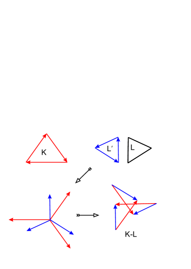
Figure 6. Minkowski difference of two polygons

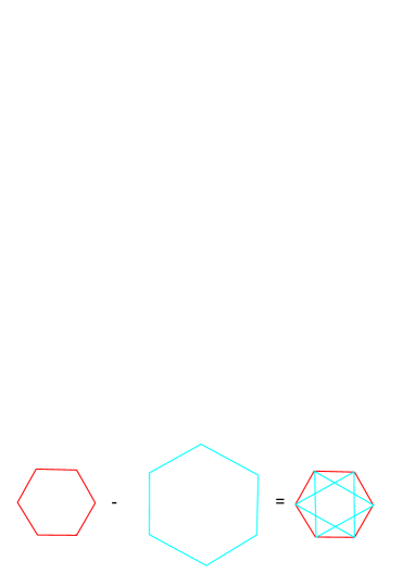
Figure 7. Minkowski difference of the polygons

$$\sum_{1\geq i>j\geq 3}q_{ij}\hbox{ and }\sum_{i=1}^{3}r_{i}.$$

Algorithm 1.

In $\mathbb{R}^{2}$, virtual polytopes can be visualized as closed polygonal chains according a simple algorithm. For polygons with mutually non-parallel edges (this is what we have in the definition of cyclopermutohedron), it runs as follows.

1. To compute $K-L$, orient the polygons $K$ and the symmetric image $L^{\prime}$ of $L$ clockwise and counterclockwise respectively.

2. Take the (oriented) edges of $K$ and $L^{\prime}$ apart and order them by the slope.

3. Following the ordering, compose a closed polygonal chain, as is shown in Figure 6.

Example 6.

For the particular case of Example 4, the algorithm gives us Figure 7. Observe that if we generically perturb one of the summands, the sum would have (instead of six) twelve vertices.

Faces of virtual polytopes

Similar to convex polytopes, the virtual polytopes also have well defined faces together with incidence relations.

To explain it,we first define in an appropriate way faces of convex polytopes.

Definition 6.

Let $K\subset\mathbb{R}^{n}$ be a convex polytope, and $\xi$ be a vector in $\mathbb{R}^{n}$. The polytope $K^{\xi}$ is the subset of $K$ where the scalar product $(\cdot,\xi)$ attains its maximal value:

$$K^{\xi}=\{x\in K|\ \forall y\in K,\ (x,\xi)\geq(y,\xi)\}.$$

$K^{\xi}$ is called the face of $K$ with the normal vector $\xi$, or the face of $K$ in direction $\xi$. If $\xi$ is a non-zero vector, we get a proper face of the polytope.

Proposition 3.

1. A face of a convex polytope is a convex polytope.

2. A face of a face of $K$ is again a face of $K$.

3. A face in the direction $\xi$ of a Minkowski sum of two convex polytopes is the Minkowski sum of the faces in direction $\xi$ from the summands:

   $(K+L)^{\xi}=K^{\xi}+L^{\xi}$.

The item (3) of the above proposition motivates us to define faces for virtual polytopes:

Definition 7.

Given a virtual polytope $K=L-M\in\mathcal{P}$, where $K$ and $L$ are convex polytopes, and $\xi\in\mathbb{R}^{n}$, the face $K^{\xi}$ is defined by

$$K^{\xi}=(L-M)^{\xi}:=L^{\xi}-M^{\xi}.$$

As in the convex case, we rank the faces by their dimensions. The $k$-dimensional faces are called $k$-faces; the $0$-faces and the $1$-faces are called vertices and edges respectively.

The faces of virtual polytopes satisfy properties similar to the convex case:

Proposition 4.

[6]

1. A face of a virtual polytope is a virtual polytope.

2. A face of a face of a virtual polytope $K$ is again a face of $K$.

3. ”Face of the sum is sum of faces”.

   $$(K+L)^{\xi}=K^{\xi}+L^{\xi}\hbox{, and }(-K)^{\xi}=-(K^{\xi}).\qed$$

Proposition 5.

For a virtual polytope $K$ and its face $F$, the faces of $F$ can be obtained in the following way.

1. Take all possible $\xi$ such that $F=K^{\xi}$.

2. Perturb $\xi$, that is, take all vectors $\eta$ that are sufficiently close to $\xi$.

3. For all those $\eta$, take $K^{\eta}$. All the resulted virtual polytopes give the set of faces of $F$.

Proof. The statement is true for convex polytopes and extends by linearity to virtual polytopes as well.∎

References

- [1] F. Chapoton, S. Fomin and A. Zelevinsky, Polytopal Realizations of generalized associahedra, Canad. Math. Bull. 45 (2003), 537–566.
- [2] I.Gelfand, M. Kapranov, A. Zelevinskii, Discriminants, Resultants and Multidimensional Determinants, Birkhauser, Boston, 1994.
- [3] M. Farber and D. Schütz, Homology of planar polygon spaces, Geom. Dedicata, 125 (2007), 75-92.
- [4] M. Kapranov, The permutoassociahedron, Mac Lane’s coherence theorem and asymptotic zones for the KZ equation, Journal of Pure and Applied Algebra, Vol. 85, 2 (1993), 119–142.
- [5] A. Khovanskii and A. Pukhlikov, Finitely additive measures of virtual polytopes, St. Petersburg Math. J., Vol. 4, 2 (1993), 337-356.
- [6] G. Panina, Virtual polytopes and some classical problems, St. Petersburg Math. J., Vol. 14, 5 (2003), 823–834.
- [7] G. Panina, New counterexamples to A.D. Alexandrov’s uniqueness hypothesis, Advances in Geometry, Vol. 5, 2 (2005), 301-317.
- [8] G. Panina, Arifmetika mnogogrannikov (in Russian), Kvant, Vol. 4, (2010), 8-13. http://www.kvant.info/k/2009/4/01-10.pdf
- [9] G. Panina, Moduli space of a planar polygonal linkage: a combinatorial description, arXiv:1209.3241
- [10] A. Postnikov,Permutohedra, Associahedra, and Beyond, Int Math Res Notices Vol. 2009 (2009), 1026-1106.
- [11] G.M. Ziegler, Lectures on polytopes, Graduate Texts in Mathematics. (Springer, Berlin 1995).