Halo Mass Definition and Multiplicity Function

Abstract

Comparing the excursion set and CUSP formalisms for the derivation of the halo mass function, we investigate the role of the mass definition in the properties of the multiplicity function of cold dark matter (CDM) haloes. We show that the density profile for haloes formed from triaxial peaks that undergo ellipsoidal collapse and virialisation is such that the ratio between the mean inner density and the outer local density is essentially independent of mass. This causes that, for suited values of the spherical overdensity $\Delta$ and the linking length $b$, SO and FoF masses are essentially equivalent to each other and the respective multiplicity functions are essentially the same. The overdensity for haloes having undergone ellipsoidal collapse is the same as if they had formed according to the spherical top-hat model, which leads to a value of $b$ corresponding to the usual virial overdensity, $\Delta_{\rm vir}$, equal to $\sim 0.2$. The multiplicity function resulting from such mass definitions, expressed as a function of the top-hat height for spherical collapse, is very approximately universal in all CDM cosmologies. The reason for this is that, for such mass definitions, the top-hat density contrast for ellipsoidal collapse and virialisation is close to a universal value, equal to $\sim 0.9$ times the usual top-hat density contrast for spherical collapse.

1 INTRODUCTION

Large scale structure harbours important cosmological information. However, such a fundamental property as the halo mass function (MF) is not well-established yet. Besides the lack of an accurate description of non-linear evolution of density fluctuations, there is the uncertainty arising from the fact that the boundary of a virialised halo is a fuzzy concept. As a consequence, the halo mass function depends on the particular mass definition adopted, its shape being only known in a few cases and over limited mass and redshift ranges.

The various halo mass definitions found in the literature arise from the different halo finders used in simulations (Knebe et al., 2011). For instance, in the Spherical Overdensity (SO) definition (Lacey & Cole, 1994), the mass of a halo at the time $t$ is that leading to a total mean density $\bar{\rho}_{\rm h}(R_{\rm h})$ equal to a fixed, constant or time-varying, overdensity $\Delta$ times the mean cosmic density $\bar{\rho}(t)$,

$$\bar{\rho}_{\rm h}(R_{\rm h})=\Delta\bar{\rho}(t)\,.$$ (1)

While in the Friends-of-Friends (FoF) definition (Davis et al., 1985), the mass of a halo is the total mass of its particles, identified by means of a percolation algorithm with fixed linking length $b$ in units of the mean inter-particle separation.

The main drawback of the FoF definition is that, for large values of $b$, it tends to over-link haloes. Its main advantage is that it can be applied without caring about the symmetry and dynamical state of haloes. Haloes are, indeed, triaxial rather than spherically symmetric, harbour substantial substructure and may be undergoing a merger, which complicates the use of the SO definition. However, one can focus on virialised objects and consider the spherically averaged density profile $\rho_{\rm h}(r)$ and mass profile $M(r)$ around the peak-density, in which case the FoF mass coincides with the mass inside the radius $R_{\rm h}$ where spheres of radius $b$ harbour two particles in average (Lacey & Cole, 1994),

$$\rho_{\rm h}(R)=\frac{3}{2\pi}\,b^{-3}\bar{\rho}(t)\,.$$ (2)

Equations (1) and (2) imply the relation

$$\Delta=\frac{3F(c)}{2\pi}\,b^{-3}\,,$$ (3)

between $\Delta$ and $b$ for haloes of a given mass $M$, where $F(c)\equiv\bar{\rho}_{\rm h}(R_{\rm h})/\rho_{\rm h}(R_{\rm h})$ is a function of halo concentration $c$.

As $c$ depends on $M$, there is no pair of $\Delta$ and $b$ values satisfying equation (3) for all $M$ at the same time. Consequently, there is strictly no equivalent SO and FoF mass definitions (More et al., 2011). Yet, numerical simulations show that, at least in the Standard Cold Dark Matter (SCDM) cosmology, FoF masses with $b=0.2$, from now on simply FoF(0.2), tightly correlate with SO masses with overdensity $\Delta$ equal to the so-called virial value, $\Delta_{\rm vir}\approx 178$, from now on SO($\Delta_{\rm vir}$) (Cole & Lacey, 1996). This correlation is often interpreted as due to the fact that haloes are close to isothermal spheres, for which $F(c)$ is equal to 3, so equation (3) for $b=0.2$ implies $\Delta\approx 178$.

Simulations also show that, in any cold dark matter (CDM) cosmology, FoF(0.2) haloes have a multiplicity function that, expressed as a function of the top-hat height for spherical collapse, is approximately universal (Jenkins et al., 2000; White, 2002; Warren et al., 2006; Lukić et al., 2007; Tinker et al., 2008; Crocce et al., 2010) and very similar to that found for SO($\Delta_{\rm vir}$) haloes (Jenkins et al., 2000; White, 2002). As $\Delta_{\rm vir}$ may substantially deviate from 178 depending on the cosmology, such a similarity cannot be due to the roughly isothermal structure of haloes as suggested by the SCDM case. Moreover, the universality of this multiplicity function is hard to reconcile with the dependence on cosmology of halo density profile (Courtin et al., 2011). On the other hand, haloes do not form through spherical collapse but through ellipsoidal collapse. For all theses reasons, the origin of such properties is unknown. Having a reliable theoretical model of the halo MF would be very useful for trying to clarify these issues.

Assuming the spherical collapse of halo seeds, Press & Schechter (1974) derived a MF that is in fair agreement with the results of numerical simulations (e.g. Efstathiou et al. 1988; White et al. 1993; Lacey & Cole 1994; Bond & Myers 1996), although with substantial deviations at both mass ends (Lacey & Cole, 1994; Gross et al., 1998; Jenkins et al., 2001; White, 2002; Reed et al., 2003; Heitmann et al., 2006). An outstanding characteristic of the associated multiplicity function is its universal shape as a function of the height of density fluctuations. Whether this characteristic is connected with the approximately universal multiplicity function of simulated haloes for FoF(0.2) masses is however hard to tell.

Bond et al. (1991) re-derived this MF making use of the so-called excursion set formalism in order to correct for cloud-in-cloud (nested) configurations. This formalism was adopted in subsequent refinements carried out with the aim to account for the more realistic ellipsoidal collapse (Monaco, 1995; Lee & Shandarin, 1998; Sheth & Tormen, 2002). The excursion set formalism has also recently been modified (Paranjape et al., 2012; Paranjape & Sheth, 2012) to account for the fact that density maxima (peaks) in the initial density field are the most probable halo seeds (Hahn & Paranjape 2013).

In an alternative approach, the extension to peaks was directly attempted from the original Press-Schechter MF (Bond, 1989; Colafrancesco et al., 1989; Peacock & Heavens, 1990; Appel & Jones, 1990; Bond & Myers, 1996; Hanami, 2001). The most rigorous derivation along this line was by Manrique and Salvador-Solé (1995, hereafter MSS; see also Manrique et al. 1998), who applied the so-called ConflUent System of Peak trajectories (CUSP) formalism, based on the Ansatz suggested by spherical collapse that “there is a one-to-one correspondence between haloes and non-nested peaks”.

A common feature of all these derivations is that they assume monolithic collapse or pure accretion. While in hierarchical cosmologies there are certainly periods in which haloes evolve by accretion, major mergers are also frequent and cannot be neglected. We will comeback to this point at the end of the paper. A second and more important issue in connection with the problem mentioned above is that none of these theoretical MFs makes any explicit statement on the halo mass definition presumed, so the specific empirical MF they are to be compared with is unknown.

Recently, Juan et al. (2013, hereafter JSDM) have shown that, combining the CUSP formalism with the exact follow-up of ellipsoidal collapse and virialisation developed by Salvador-Solé et al. (2012, hereafter SVMS), it is possible to derive a MF that adapts to any desired halo mass definition and is in excellent agreement with the results of simulations.

In the present paper, we use the excursion set and CUSP formalisms to explain the origin of the observed properties of the halo multiplicity function.

In Section 2, we recall the two different approaches for the derivation of the MF. In Section 3, we investigate the mass definition implicitly assumed in such approaches. The origin of the similarity of the multiplicity function for FoF(0.2) and SO($\Delta_{\rm vir}$) masses and of its approximate universality is addressed in Sections 4 and 5, respectively. Our results are discussed and summarised in Section 6.

All the quantitative results given throughout the paper are for the concordant $\Lambda$CDM cosmology with $\Omega_{\Lambda}=0.73$, $\Omega_{\rm m}=0.23$, $\Omega_{\rm b}=0.045$, $H_{0}=0.71$ km s^-1 Mpc^-1, $\sigma_{8}=0.81$, $n_{\rm s}=1$ and Bardeen et al. (1986, hereafter BBKS) CDM spectrum with Sugiyama (1995) shape parameter.

2 Mass Function

All derivations of the halo MF proceed by first identifying the seeds of haloes with mass $M$ at the time $t$ in the density field at an arbitrary small enough cosmic time $t_{\rm i}$ and then counting those seeds.

2.1 The Excursion Set Formalism

In this approach, halo seeds are assumed to be spherical overdense regions in the initial density field smoothed with a top-hat filter that undergo spherical collapse.

The time of spherical collapse (neglecting shell-crossing) of a seed depends only on its density contrast, so there is a one-to-one correspondence between haloes with $M$ at $t$ and density perturbations with fixed density contrast $\delta_{\rm ci}$ at the filtering radii ${R_{\rm f}}$ satisfying the relations

$$\delta_{\rm ci}(t)=\delta_{\rm c}(t)\frac{D(t_{\rm i})}{D(t)}\,$$ (4)

$${R_{\rm f}}(M)=\left[\frac{3M}{4\pi\bar{\rho}_{\rm i}}\right]^{1/3}\,.$$ (5)

In equations (4) and (5), $\bar{\rho}_{\rm i}$ is the mean cosmic density at $t=t_{\rm i}$, $\delta_{\rm c}(t)$ is the almost universal density contrast for spherical collapse at $t$ linearly extrapolated to that time and $D(t)$ is the cosmic growth factor. In the Einstein-de Sitter universe, $D(t)$ is equal to the cosmic scale factor $a(t)$ and $\delta_{\rm c}(t)$ is equal to $3(12\pi)^{2/3}/20\approx 1.686$. While, in the concordant model and the present time $t_{0}$, $D(t_{0})$ is a factor 0.760 smaller than $a(t_{0})$ and $\delta_{\rm c}(t_{0})$ is equal to $\approx 1.674$ (e.g. Henry 2000).

Equation (5) is valid to leading order in the perturbation, the exact relation between ${R_{\rm f}}$ and $M$ being

$${R_{\rm f}}(M,t)=\left\{\frac{3M}{4\pi\bar{\rho}_{\rm i}[1+\delta_{\rm ci}(t)]}\right\}^{1/3}\,.$$ (6)

The interest of adopting the approx relation (5) is that the filtering radius then depends only on $M$. This greatly simplifies the mathematical treatment.

Following Press & Schechter (1974), every region with density contrast greater than or equal to $\delta_{\rm ci}(t)$ at the scale ${R_{\rm f}}(M)$ will give rise at $t$ to a halo with mass greater than or equal to $M$. Consequently, the MF, i.e. the comoving number density of haloes per infinitesimal mass around $M$ at $t$, is simply the $M$-derivative of the volume fraction occupied by those regions, equal in Gaussian random density fields to

$$V(M,t)=\frac{1}{2}\,{\rm erfc}\left[\frac{1}{\sqrt{2}}\,\frac{\delta_{\rm ci}(t)}{\sigma_{0}^{\rm th}(M,t_{\rm i})}\right]\,,$$ (7)

divided by the volume $M/\bar{\rho}(t)$ of one single seed,

$$\frac{\partial n_{\rm PS}(M,t)}{\partial M}=\frac{\bar{\rho}(t)}{M}\,\frac{\partial V(M,t)}{\partial M}\,.$$ (8)

In equation (7), $\sigma_{0}^{\rm th}(M,t_{\rm i})$ is the top-hat rms density fluctuation of scale $M$ at $t_{\rm i}$.

But this derivation does not take into account that overdense regions of a given scale may lie within larger scale overdense regions, which translates into a wrong normalisation of the MF (7)–(8). To correct for this effect, Bond et al. (1991) introduced the excursion set formalism. The density contrast $\delta$ at any fixed point tends to decrease as the smoothing radius ${R_{\rm f}}$ increases, so, using a sharp k-space filter, $\delta$ traces a Brownian random walk, easy to monitor statistically. In particular, one can estimate the number of haloes reaching $M$ at $t$ by counting the excursion sets $\delta(R)$ intersecting $\delta_{\rm ci}(t)$ at any scale ${R_{\rm f}}(M)$. The important novelty of this approach is that, whenever a halo undergoes a major merger, $\delta$ increases instead of decreasing, so every trajectory $\delta(R)$ can intersect $\delta_{\rm ci}(t)$ at more than one radius $R$, meaning that there will be haloes appearing within other more massive ones. Therefore, to correct for cloud-in-cloud configurations, one must simply count the excursion sets intersecting $\delta_{\rm ci}(t)$ for the first time as $R$ decreases from infinity (or $\sigma_{0}^{\rm th}$ increases from zero), as if they were absorbed at such a barrier. The MF so obtained has identical form as the Press-Schechter one (eqs. [8]-[7]) but with an additional factor two,

$$\frac{\partial n_{\rm es}(M,t)}{\partial M}=2\frac{\partial n_{\rm PS}(M,t)}{\partial M}\,,$$ (9)

yielding the right normalisation of the excursion set MF.

Note that, as the height of a density fluctuation, defined as the density contrast normalised to the rms value at the same scale, is constant with time, the volume $V(M,t)$ (eq. [7]) can be written as a function of $\nu_{\rm es}=\delta_{\rm ci}(t)/\sigma_{0}^{\rm th}(M,t_{\rm i})=\delta_{\rm c}(t)/\sigma_{0}^{\rm th}(M,t)=\delta_{\rm c0}(t)/\sigma_{0}^{\rm th}$, where $\delta_{\rm c0}(t)$ is $\delta_{\rm c}(t)D(t_{0})/D(t)$ and $\sigma_{0}^{\rm th}$ stands for the 0th order spectral moment at the current time $t_{0}$. Thus, the resulting MF (eq. [8]) is independent of the arbitrary initial time $t_{\rm i}$.

But the assumptions made in this derivation are not fully satisfactory: i) Every overdense region does not collapse into a distinct halo; only those around peaks do. Unfortunately, the extension of the excursion set formalism to peaks is not trivial (Paranjape et al., 2012; Paranjape & Sheth, 2012); ii) Real haloes (and peaks) are not spherically symmetric but triaxial, so halo seeds do not undergo spherical but ellipsoidal collapse. Unfortunately, the implementation in this approach of ellipsoidal collapse is hard to achieve due to the dependence on $M$ of the corresponding critical density contrast (Sheth & Tormen, 2002; Paranjape et al., 2012; Paranjape & Sheth, 2012). iii) The formation of haloes involves not only the collapse of the seed, but also the virialisation (through shell-crossing) of the system, which is hard to account for. And iv) there is a slight inconsistency between the top-hat filter used to monitor the dynamics of collapse and the sharp k-space window used to correct for nesting. The use of the top-hat filter with this latter purpose is again hard to implement due to the correlation between fluctuations at different scales in top-hat smoothing (Musso & Paranjape, 2012).

2.2 The CUSP Formalism

In this approach, halo seeds are regions around non-nested (triaxial) peaks that undergo ellipsoidal collapse and virialisation. The use of a Gaussian filter is mandatory in this case for the reasons given below.

The time of collapse and virialisation of triaxial seeds depends not only on their density contrast $\delta$ at the suited scale $R$, like in spherical collapse, but also on their ellipticity and density slope (e.g. Peebles 1980). However, all peaks with given $\delta$ at $R$ have similar ellipticities and density slopes (JSDM). Consequently, all haloes at $t$ can be seen to arise from non-nested triaxial peaks at $t_{\rm i}$ with the same fixed density contrast $\delta_{\rm mi}$ at any filtering radius ${R_{\rm f}}$. Then, taking advantage of the freedom in the boundary of virialised haloes, we can adopt at $t$ a suited mass definition so to exactly match the one-parameter family of resulting halo masses $M({R_{\rm f}},t)$. By doing this, we will end up with a one-to-one correspondence between haloes with $M$ at $t$ and non-nested (triaxial) peaks at $t_{\rm i}$ with $\delta_{\rm mi}$ at ${R_{\rm f}}$, according to the relations

$$\delta_{\rm mi}(t)=\delta_{\rm m}(t)\frac{D(t_{\rm i})}{D(t)}\,$$ (10)

$${R_{\rm f}}(M,t)=\frac{1}{q(M,t)}\left[\frac{3M}{4\pi\bar{\rho}_{\rm i}}\right]^{1/3}\,.$$ (11)

Equations (10)–(11) are very similar to equations (4)–(5). However, the pair of functions $\delta_{\rm m}(t)$ and $q(M,t)$ are now arbitrary, fixing one particular halo mass definition each (and conversely; see Sec. 3.2). For this reason the subindex “c” for “collapse” in the density contrasts appearing in the relation (4) has been replaced by the subindex “m” indicating that the masses of haloes at $t$ “match” a certain definition. The only constraints these two functions must fulfil, for consistency with the mass growth of haloes, are: $\delta_{\rm mi}(t)$ must be a decreasing function of time and ${R_{\rm f}}(M,t)$ must be an increasing function of mass. That consistency condition is precisely what makes the use of the Gaussian filter mandatory. Such a filter is indeed the only one guaranteeing, through the relation $R\nabla^{2}\delta=\partial\delta/\partial R$, that the density contrast $\delta$ of peaks necessarily decreases as the filtering radius $R$ increases, in agreement with the evolution of halo masses.

The radius $R_{\rm p}$ of the spherically averaged seed (or protohalo) with $M$ is now different from the Gaussian filtering radius ${R_{\rm f}}$. It is instead equal to $q_{\rm p}{R_{\rm f}}$, with $q_{\rm p}$ satisfying the relation

$${R_{\rm f}}(M,t)=\frac{1}{q_{\rm p}(M,t)}\left\{\frac{3M}{4\pi\bar{\rho}_{\rm i}[1+\delta_{\rm mi}^{\rm th}(M,t)]}\right\}^{1/3},$$ (12)

where $\delta_{\rm mi}^{\rm th}(M,t)$ is the density contrast of the peak when the density field is smoothed with a top-hat filter encompassing the same mass $M$, related to the (unconvolved) spherically averaged density contrast profile of the seed $\delta_{\rm p}(r)$ through

$$\delta_{\rm mi}^{\rm th}(M,t)=\frac{3}{R_{\rm p}^{3}}\int_{0}^{R_{\rm p}}{\rm d}r\,r^{2}\,\delta_{\rm p}(r)\,.$$ (13)

But factors $[1+\delta_{\rm mi}^{\rm th}(M,t)]^{1/3}$ and $q_{\rm p}(M,t)$ on the right of equation (12) can be absorbed in the function $q(M,t)$. Thus, contrarily to the relation (5), equation (11) is exact. Note that $q(M,t)$ is then, to leading order in the perturbation as in equation (5), the radius $R_{\rm p}$ of the seed in units of the Gaussian filtering radius ${R_{\rm f}}$.

We emphasise that, owing to the Gaussian smoothing, the radius of the filter ${R_{\rm f}}$ depends, in the CUSP formalism, not only on $M$ but also on $t$ through $q(M,t)$, while $\delta_{\rm mi}$ and, hence, $\delta_{\rm m}$ are still functions of $t$ alone. This latter functionality may seem contradictory with the fact that, as pointed out by Sheth & Tormen (2002) and recently checked with simulations (e.g., Robertson et al. 2009; Elia et al. 2012; Despali et al. 2013; Hahn & Paranjape 2013), the density contrast for ellipsoidal collapse depends on the mass of the perturbation. There is however no contradiction. The CUSP formalism uses a Gaussian filter instead of a top-hat filter like in all these works and this difference is crucial because of the freedom introduced by $q(M,t)$. In top-hat smoothing, $q$ is fixed to one, so considering ellipsoidal collapse necessarily translates into a value of $\delta_{\rm c}$ dependent on $M$ in addition to $t$. While, in Gaussian smoothing, we can impose that the density contrast for collapse is independent of $M$ and let $q$ depend on $M$ and $t$. Note that, when the density field at $t_{\rm i}$ is smoothed with a top-hat filter, the density contrast of halo seeds, $\delta_{\rm mi}^{\rm th}(M,t)$, is indeed a function of $M$ and $t$ in general. The exact way $\delta_{\rm mi}^{\rm th}(M,t)$ depends on $M$ will depend, of course, on the mass definition used.

We are now ready to calculate the MF in this approach. Given the one-to-one correspondence between haloes and non-nested peaks, the counting of haloes with $M$ at $t$ reduces to count non-nested peaks with that scale at $t_{\rm i}$. In the original version of the CUSP formalism (MSS), such a counting did not take into account the correlation between peaks at different scales. However, the more accurate version later developed (Manrique et al., 1998) yielded essentially the same result, so we will follow here that simple version (see the Appendix for the more accurate one). For simplicity, we will omit hereafter any subindex in the Gaussian rms density fluctuation $\sigma_{0}$ and in the CUSP height $\nu\equiv\delta_{\rm mi}/\sigma_{0}(M,t_{\rm i})=\delta_{\rm m}(t)/\sigma_{0}(M,t)=\delta_{\rm m0}(t)/\sigma_{0}$, where $\delta_{\rm m0}(t)$ is $\delta_{\rm m}(t)D(t_{0})/D(t)$ and $\sigma_{0}$ stands for the 0th order spectral moment at $t_{0}$. The subindexes “th” and “es” in the excursion set counterparts are enough to tell between the two sets of variables.

The number density of peaks with $\delta_{\rm mi}$ per infinitesimal $\ln\sigma_{0}^{-1}(M,t_{\rm i})$ at $t_{\rm i}$ or, equivalently, with $\delta_{\rm m0}$ per infinitesimal $\ln\sigma_{0}^{-1}$ at $t_{0}$ can be readily calculated from the density of peaks per infinitesimal height around $\nu$, derived by BBKS. The result is

$$N(\sigma_{0},\delta_{\rm m0})=\frac{\langle x\rangle\!(\sigma_{0},\delta_{\rm m0})}{(2\pi)^{2}\,R_{\star}^{3}\,\gamma}\,\,{\rm e}^{-\frac{\nu^{2}}{2}}\,,$$ (14)

where $R_{\star}$ and $\gamma$ are respectively defined as $\sqrt{3}\sigma_{1}/\sigma_{2}$ and $\sigma_{1}^{2}/(\sigma_{0}\sigma_{2})$, being $\sigma_{j}$ the $j$-th order (Gaussian) spectral moment, and $\left\langle x\right\rangle\!(\sigma_{0},\delta_{\rm m0})$ is the average curvature (i.e. minus the Laplacian scaled to the mean value $\sigma_{2}$) of peaks with $\delta_{\rm m0}$ and $\sigma_{0}$, well-fitted by the analytic expression (BBKS)

$$\langle x\rangle(\nu)=\gamma\nu+\frac{3(1-\gamma^{2})+(1.216-0.9\gamma^{4}){\rm e}^{-\frac{\gamma}{2}\,\left(\frac{\gamma\nu}{2}\right)^{2}}}{\left[3(1-\gamma^{2})+0.45+(\gamma\nu/2)^{2}\right]^{1/2}+\gamma\nu/2}\,.$$ (15)

But this number density is not enough for our purposes because we are interested in counting non-nested peaks only. The homologous number density of non-nested peaks, $N^{\rm nn}(\sigma_{0},\delta_{\rm m0})$, can be obtained by solving the Volterra integral equation

$$N^{\rm nn}(\sigma_{0},\delta_{\rm m0})=N(\sigma_{0},\delta_{\rm m0})-\!\!\int_{\ln\sigma_{0}^{-1}}^{\infty}{\rm d}\ln{\sigma^{\prime}_{0}}^{-1}~{}~{}~{}~{}~{}~{}~{}$$

$$\times N(\sigma_{0},\delta_{\rm m0}|\sigma^{\prime}_{0},\delta_{\rm m0})\frac{M(\sigma^{\prime}_{0},\delta_{\rm m0})}{\bar{\rho}}N^{\rm nn}(\sigma^{\prime}_{0},\delta_{\rm m0}),$$ (16)

where the second term on the right gives the density of peaks with $\delta_{\rm m0}$ per infinitesimal $\ln\sigma_{0}^{-1}$ nested into peaks with identical density contrast at larger scales, $\ln{\sigma^{\prime}_{0}}^{-1}$. The conditional number density $N(\sigma_{0},\delta_{\rm m0}|\sigma^{\prime}_{0},\delta_{\rm m0})$ of peaks with $\delta_{\rm m0}$ per infinitesimal $\ln\sigma_{0}^{-1}$ subject to lying in backgrounds with $\delta_{\rm m0}$ at $\sigma^{\prime}_{0}<\sigma_{0}$ can also be calculated from the conditional number density per infinitesimal $\nu$ in backgrounds with $\nu^{\prime}$ derived by BBKS. The result is

$$N(\sigma_{0},\delta_{\rm m0}|\sigma^{\prime}_{0},\delta_{\rm m0})=\frac{\langle x\rangle(\tilde{\sigma}_{0},\delta_{\rm m0})}{(2\pi)^{2}\,R_{\star}^{3}\,\gamma\,\sqrt{1-\epsilon^{2}}}\,{\rm e}^{-\frac{(\nu-\epsilon\,\nu^{\prime})^{2}}{2(1-\epsilon^{2})}}\,,$$ (17)

where $\nu^{\prime}$ and $\epsilon$ are respectively defined as $\delta_{\rm m0}/\sigma_{0}^{\prime}$ and $\sigma_{0}^{2}(R_{\rm m})/[\sigma_{0}\sigma^{\prime}_{0}]$, being $R_{\rm m}^{2}$ equal to the arithmetic mean of the squared filtering radii corresponding to $\sigma_{0}$ and $\sigma_{0}^{\prime}$, and where $\langle x\rangle\!(\tilde{\sigma}_{0},\delta_{\rm m0})$ takes the same form (15) as $\langle x\rangle\!(\sigma_{0},\delta_{\rm m0})$ in equation (14) but as a function of $\tilde{\gamma}\tilde{\nu}$ instead of $\gamma\nu$, being

$$\tilde{\gamma}^{2}=\gamma^{2}\left[1+\epsilon^{2}\,{(1-r_{1})^{2}\over 1-\epsilon^{2}}\right]$$ (18)

$$\tilde{\nu}(r)\!=\!{\gamma\over\tilde{\gamma}}\,{1-r_{1}\over 1-\epsilon^{2}}\left[\nu\!\left({1-\epsilon^{2}r_{1}\over 1-r_{1}}\!\right)\!-\epsilon\nu^{\prime}\right]\!,$$ (19)

with $r_{1}$ equal to $[\sigma_{0}({R_{\rm f}})\sigma_{1}(R_{\rm m})/(\sigma_{1}({R_{\rm f}})\sigma_{0}(R_{\rm m}))]^{2}$.

Thus, the MF of haloes at $t$ is then

$$\frac{\partial n_{\rm CUSP}(M,t)}{\partial M}=\,N^{\rm nn}[\sigma_{0},\delta_{\rm m0}]\,\frac{\partial\ln\sigma_{0}^{-1}}{\partial M}\,.$$ (20)

Note that this expression of the MF is also independent of the (arbitrary) initial time $t_{\rm i}$.

The CUSP formalism thus solves all the problems met in the excursion set formalism: it deals with triaxial peaks that undergo ellipsoidal collapse and virialisation, conveniently corrected for nesting, and the smoothing of the initial density field is always carried out with the same Gaussian filter. The only drawback of this approach is the need to solve the Volterra equation (16), which prevents from having an analytic expression for the resulting MF.

3 Implicit Halo Mass Definition

For any theoretical MF to be complete, the mass definition it refers to must be specified. In other words, one must state the condition defining the total radius $R_{\rm h}$ or, equivalently, the spherically averaged density profile for haloes with different masses at $t$ that result from the specific halo seeds and dynamics of collapse assumed.

3.1 The Excursion Set Formalism

In the excursion set formalism, halo seeds are arbitrary overdense regions with no definite inner structure, so their typical (mean) density and peculiar velocity fields are uniform. As a consequence, the density distribution in the corresponding final virialised objects is also uniform. In addition, the system is supposed to undergo spherical collapse. Therefore, halo formation is according to the simple spherical top-hat model, in which case the typical radii $R_{\rm h}$ of haloes with different masses at $t$ can be readily inferred (Peebles, 1980).

The virial relation $2T+W=0$ holding for the final uniform object together with energy conservation imply that $R_{\rm h}$ is half the radius of the uniform system at turnaround. This leads to

$$R_{\rm h}=-\frac{3GM^{2}}{10E_{\rm p}(M)}\,,$$ (21)

where $E_{\rm p}(M)$ is the (conserved) total energy of the protohalo with mass $M$. Taking into account that $E_{\rm p}$ is, to leading order in the perturbation, equal to $-\delta_{\rm ci}(t)GM^{2}/{R_{\rm f}}$ (see eqs. [30]–[29] for $\rho_{\rm p}=\bar{\rho}_{\rm i}[1+\delta_{\rm ci}(t)]$), equation (21) takes the form

$$R_{\rm h}=\left[\frac{3M}{4\pi\Delta_{\rm vir}(t)\bar{\rho}(t)}\right]^{1/3}\,$$ (22)

or, equivalently,

$$\bar{\rho}_{\rm h}(R_{\rm h})=\Delta_{\rm vir}(t)\,\bar{\rho}(t)\,,$$ (23)

where we have introduced the so-called virial overdensity corresponding to the spherical top-hat model,

$$\Delta_{\rm vir}(t)\equiv\left[\frac{10\,\delta_{\rm c}(t)a(t)}{3\,D(t)}\right]^{3}\,.$$ (24)

Comparing equations (1) and (23), we see that the halo mass definition implicitly presumed in the excursion set formalism is the SO($\Delta_{\rm vir}$) one, with $\Delta_{\rm vir}$ dependent on time and cosmology. In the Einstein-de Sitter universe, where $\delta_{\rm c}(t)$ is equal to $3(12\pi)^{2/3}/20$ and $D(t)=a(t)$, $\Delta_{\rm vir}(t)$ takes the constant value $18\pi^{2}\approx 178$. While, at $t_{0}$ in the concordant model, where $\delta_{\rm c}(t_{0})$ and $D(t_{0})$ are respectively equal to $\approx 1.674$ and $\approx 0.760$, $\Delta_{\rm vir}(t_{0})$ takes the value $\approx 359$ (Henry, 2000).

3.2 The CUSP Formalism

In ellipsoidal collapse, the total energy $E_{\rm p}$ of a sphere with mass $M$ is not conserved. On the other hand, for peaks (hence, with outwards decreasing density profiles) shells exchange energy as they cross each other, causing virialisation to progress from the centre of the system outwards. Thus, the spherical top-hat model does not hold. However, as shown in SVMS, one can still accurately derive the typical density profile $\rho_{\rm h}(r)$ for haloes.

The variation in time of the total energy of a sphere undergoing ellipsoidal collapse compared to that of the spherically averaged system can be accurately monitored. In addition, during virialisation, there is no apocentre-crossing (despite there being shell-crossing), which causes virialised haloes to develop from the inside out, keeping the instantaneous inner structure unchanged. In these conditions, the radius $r$ encompassing any given mass $M$ in the final triaxial virialised system exactly satisfies the relation

$$r=-\frac{3GM^{2}}{10E_{\rm p}(M)},$$ (25)

identical, at every radius $r$, to the relation (21) holding for the whole object in the excursion set case.

In equation (25), $E_{\rm p}(M)$ is the (now non-conserved) energy distribution of the spherically averaged protohalo. In the parametric form, it is given by

$$E_{\rm p}(r)=4\pi\!\int_{0}^{r}\!\!{\rm d}\tilde{r}\,\tilde{r}^{2}\rho_{\rm p}(\tilde{r})\!\left\{\!\frac{\left[H_{\rm i}\tilde{r}-v_{\rm p}(\tilde{r})\right]^{2}}{2}\!-\!\frac{GM(\tilde{r})}{\tilde{r}}\!\right\}$$ (26)

$$M(r)=4\pi\!\int_{0}^{r}{\rm d}\tilde{r}\,\tilde{r}^{2}\,\rho_{\rm p}(\tilde{r})\,,$$ (27)

where $\rho_{\rm p}(r)=\bar{\rho}_{\rm i}[1+\delta_{\rm p}(r)]$ is the (unconvolved) spherically averaged density profile of the protohalo, $H_{\rm i}$ is the Hubble constant at $t_{\rm i}$ and

$$v_{p}(r)=\frac{2G\,\delta\!M(r)}{3H_{\rm i}r_{p}^{2}}$$ (28)

is, to leading order in the perturbation, the peculiar velocity at $r$ induced by the inner mass excess (e.g. Peebles 1980),

$$\delta\!M(r)=4\pi\int_{0}^{r}{\rm d}\tilde{r}\,\tilde{r}^{2}\,\bar{\rho}_{\rm i}\,\delta_{\rm p}(\tilde{r})\,.$$ (29)

Replacing $v_{\rm p}(r)$ given by equation (28)–(29) into equation (26), we are led to

$$E_{\rm p}(r)=-\frac{20\pi}{3}\int_{0}^{r}{\rm d}\tilde{r}\,\tilde{r}\,\rho_{\rm p}(\tilde{r})\,G\,\delta\!M(\tilde{r})\,.$$ (30)

Note that the non-null (in Eulerian coordinates) peculiar velocity $v_{\rm p}(r)$ introduces a factor 5/3 in the value of $E_{\rm p}(r)$ with respect to the one resulting in the absence of peculiar velocities. In the usual presentation (in Lagrangian coordinates) of spherical collapse, $v_{\rm p}(r)$ is null, but the initial density contrast then decomposes in the growing and decaying modes and the mass excess causing the gravitational pull in equation (28) has an extra factor 5/3 compared to the mass excess $\delta\!M(r)$ associated with the growing mode $\delta_{\rm p}$ contributing to the mass of the final halo. Consequently, the resulting value of $E_{\rm p}(r)$ is exactly the same as in equation (30).

The density contrast $\delta(R)$ of the seed of the progenitor of scale $R$ of any accreting halo with $M$ at $t$ is but the (unconvolved) spherically averaged density contrast profile $\delta_{\rm p}(r)$ of the protohalo convolved with a Gaussian window of radius $R$. We thus have

$$\delta(R)=\frac{4\pi}{(2\pi)^{3/2}R^{3}}\int_{0}^{\infty}{\rm d}r\,r^{2}\,\delta_{\rm p}(r)\,{\rm e}^{-\frac{1}{2}\left(\frac{r}{R}\right)^{2}}\,.$$ (31)

Equation (31) indicates that the trajectory $\delta(R)$ of peaks with varying scale $R$ tracing the accretion of a halo with mass $M$ at $t$ is the Laplace transform of the profile $\delta_{\rm p}(r)$ of its seed. As for haloes growing inside-out the mean density profile $\rho_{\rm h}(r)$ is determined by the mean accretion rate ${\rm d}M/{\rm d}t$ undergone over their aggregation history, the mean peak trajectory $\delta(R)$ tracing such an evolution is characterised by having the mean slope ${\rm d}R/{\rm d}\delta$ of peaks with $\delta$ at every $R$. Thus, the desired mean peak trajectory $\delta(R)$ is the solution of the differential equation

$$\frac{{\rm d}\delta}{{\rm d}R}=-\,\langle x\rangle[R,\delta(R)]\,\sigma_{2}(R)\,R\,$$ (32)

for the boundary condition $\delta[R={R_{\rm f}}(M,t)]=\delta_{\rm mi}(t)$. Once the trajectory $\delta(R)$ has been obtained, we can infer the profile $\delta_{\rm p}(r)$ by inversion of equation (31) (see SVMS for details) and use equations (27) and (30) to calculate $E_{\rm p}(M)$. Then, replacing this function into equation (25), we can infer the mass profile $M(r)$ of the halo, leading to the density profile $\rho_{\rm h}(r)$, which turns out to be in good agreement with the results of simulations (JSDM).

The mean spherically averaged halo density profile thus depends, like the MF itself, on the particular mass definition adopted through the functions $\delta_{\rm mi}(t)$ and ${R_{\rm f}}(M,t)$ or, equivalently, $\delta_{\rm m}(t)$ and $q(M,t)$, setting the boundary condition for integration of equation (32).

To obtain the halo mass definition that corresponds to any given pair of $\delta_{\rm m}(t)$ and $q(M,t)$ functions, we must calculate the density profile for haloes of different masses and find the relations $f_{1}[\rho_{\rm h}(R),M]=\bar{\rho}(t)$ and $f_{2}[\bar{\rho}_{\rm h}(R),M]=\bar{\rho}(t)$ between $\rho_{\rm h}(R)$ and $\bar{\rho}_{\rm h}(R)$ and the mean cosmic density $\bar{\rho}(t)$ for haloes with different $M$. Then, inverting, say, $f_{2}$ so as to obtain $M$ as a function of $\bar{\rho}_{\rm h}(R)$ and $\bar{\rho}(t)$ and replacing it in $f_{1}$, we are led to a relation

$$F[\rho_{\rm h}(R),\bar{\rho}_{\rm h}(R)]=\bar{\rho}(t)$$ (33)

of the general form of relations (1) and (2) setting the halo mass definition associated with the CUSP MF with arbitrary functions $\delta_{\rm m}(t)$ and $q(M,t)$.

Conversely, the functions $\delta_{\rm m}(t)$ and $q(M,t)$ can be inferred from any given halo mass definition. To do this we must impose the two following consistency arguments (JSDM): i) the total mass associated with the resulting density profile must be equal to $M$ and ii) the resulting MF must be correctly normalised. For SO($\Delta_{\rm vir}$) or FoF(0.19) masses in the concordant cosmology, JSDM found

$$\delta_{\rm m}(t)=\delta_{\rm c}(t)\frac{[a(t)]^{1.0628}}{D(t)}\,$$ (34)

and

$$q(M,t)\approx\left[Q\,\frac{\sigma_{0}^{\rm th}(M,t)}{\sigma_{0}(M,t)}\right]^{-2/(n+3)}\,.$$ (35)

In equation (35), the ratio $\sigma^{\rm th}_{0}(M,t)/\sigma_{0}(M,t)$ takes the form

$$\frac{\sigma^{\rm th}_{0}(M,t)}{\sigma_{0}(M,t)}=1-0.0682\left[\frac{D(t)}{D(t_{0})}\right]^{2}\nu\,,$$ (36)

$Q$ is defined as

$$Q^{2}\equiv\frac{\int_{0}^{\infty}{\rm d}x\,x^{n+2}\,W_{\rm G}^{2}(x)}{\int_{0}^{\infty}{\rm d}x\,x^{n+2}\,W^{2}_{\rm TH}(x)}\,,$$ (37)

where $W_{\rm th}(x)$ and $W_{\rm G}(x)$ are the Fourier transforms of the top-hat and Gaussian windows of radius $x/k$, respectively, and $n$ is the effective spectral index. The approximate relation (35) follows from the more fundamental one (36), taking into account the relation

$$\sigma^{2}_{0}({R_{\rm f}})\approx\frac{A}{2\pi^{2}}{R_{\rm f}}^{-(n+3)}\int_{0}^{\infty}{\rm d}x\,W^{2}(x)\,x^{n+2}\,,$$ (38)

holding for the 0th order spectral moment for a filter with Fourier transform $W$ under the power-law approximation, $P(k)=Ak^{n}$, of the CDM (linear) spectrum, and the fact that the Gaussian and top-hat radii for a seed with $M$ are respectively equal to ${R_{\rm f}}$ or to $q_{\rm p}{R_{\rm f}}$. This means that $Q$ and $n$ depend on the mass range considered. For the mass ranges typically covered by the MFs found in simulations, $Q$ and $n$ take values around $0.5$ and $-1.5$, respectively.

Therefore, the CUSP MF is more general than the excursion set one in the sense that it does not presume any particular mass definition; it holds for any arbitrary one, adapting to it through the functions $\delta_{\rm m}(t)$ and $q(M,t)$.

4 Similarity of SO and FoF Masses

The fact that the CUSP formalism distinguishes between different mass definitions can be used to try to understand the origin of the similarity between SO and FoF masses and their respective mass and multiplicity functions.

Equations (27) and (30) imply

$$\frac{{\rm d}E_{\rm p}}{{\rm d}M}\!=-\frac{5G\,\delta\!M(R_{\rm p})}{3R_{\rm p}}\!=-\frac{5}{3}\left[\frac{4\pi\bar{\rho}_{\rm i}}{3}\right]^{1/3}\!GM^{2/3}\delta_{\rm mi}^{\rm th}(M,t)\,,$$ (39)

where we have taken into account that the radius $R_{\rm p}$ of the protohalo is equal to $q_{\rm p}{R_{\rm f}}$ with $q_{\rm p}$ satisfying equation (12). Comparing with the $M$-derivative of equation (25) and taking into account the identity $M=4\pi\bar{\rho}_{\rm h}(R_{\rm h})R_{\rm h}^{3}/3$, equation (39) leads to the relation

$$\frac{5}{9}\left[\frac{\bar{\rho}_{\rm i}}{\bar{\rho}(t)}\right]^{1/3}\delta_{\rm mi}^{\rm th}(M,t)=\!\!\left[\frac{\bar{\rho}_{\rm h}(R_{\rm h})}{\bar{\rho}(t)}\right]^{1/3}\!\left[1-\frac{\bar{\rho}_{\rm h}(R_{\rm h})}{6\,\rho_{\rm h}(R_{\rm h})}\right]\!,$$ (40)

which, making use of the definition of $F(c)$, can be rewritten in the two following forms

$$\bar{\rho}_{\rm h}(R)=\bar{\rho}(t)\!\left[\frac{5\,\delta_{\rm mi}^{\rm th}(M,t)a(t)}{9\,a(t_{\rm i})}\right]^{3}\left[1-\frac{F(c)}{6}\right]^{-3}$$ (41)

and

$$\rho_{\rm h}(R)=\bar{\rho}(t)\!\left[\frac{5\,\delta_{\rm mi}^{\rm th}(M,t)a(t)}{9\,a(t_{\rm i})]}\right]^{3}\left[1-\frac{F(c)}{6}\right]^{-3}\frac{1}{F(c)}\,.$$ (42)

For SO and FoF masses, these expressions therefore imply

$$\Delta=\left[\frac{5\,\delta_{\rm mi}^{\rm th}(M,t)a(t)}{9\,a(t_{\rm i})}\right]^{3}\left[1-\frac{F(c)}{6}\right]^{-3}$$ (43)

and

$$b=\left[\frac{2\pi}{3F(c)}\right]^{-1/3}\left[\frac{5\,\delta_{\rm mi}^{\rm th}(M,t)a(t)}{9\,a(t_{\rm i})}\right]^{-1}\left[1-\frac{F(c)}{6}\right]\,,$$ (44)

respectively.

Equation (43) seems to indicate that, in the SO case, the mass dependence of $\delta_{\rm mi}^{\rm th}$ must cancel with that coming from $F(c)$. But equation (1) implies $R_{\rm h}\propto M^{1/3}$, which, replaced into equation (25) at $r=R_{\rm h}$, leads to $E_{\rm p}(M)\propto M^{5/3}$ and, hence, to ${\rm d}E_{\rm p}/{\rm d}M\propto M^{2/3}$, implying (see eq. [39]) that $\delta_{\rm mi}^{\rm th}$ is a function of $t$ alone. The solution to this paradox is that, to leading order in the perturbation as used in the derivation of the density profile (see eq. [28]), $\delta_{\rm mi}^{\rm th}$ and $F(c)$ are, in the SO case, independent of $M$. (Likewise, eq. [44] multiplied by the cubic root of $F(c)$ leads in the FoF case to a similar paradox, with identical solution.) Consequently, to such an order of approximation, the SO and FoF mass definitions with $\Delta$ and $b$ satisfying equation (3) are equivalent to each other.

We thus see that the origin of this approx equivalence is the inside-out growth of accreting haloes, crucial to obtain equation (25) setting the typical spherically averaged density profile for haloes arising from peaks that undergo ellipsoidal collapse and virialisation. But this is not all. We can go a step further and infer the value of $b$ leading to FoF masses equivalent to SO($\Delta_{\rm vir}$) ones.

The relation between the two functions (of $t$) $\delta_{\rm mi}^{\rm th}$ and $1-F(c)/6$ can be readily derived for the particular case of SO($\Delta_{\rm vir}$) haloes. Comparing equations (21) and (25), the latter at $r=R_{\rm h}$, we have that haloes arising from ellipsoidal collapse of peaks with $\delta_{\rm mi}$ in the density field at $t_{\rm i}$ smoothed with a Gaussian filter of radius ${R_{\rm f}}$, could have formed according to the spherical top-hat model from the same seeds with $\delta_{\rm mi}^{\rm th}$ when the density field is smoothed with a top-hat filter of radius $q{R_{\rm f}}$. Equations (24) and (43), the latter for $\Delta=\Delta_{\rm vir}$, then imply

$$\delta_{\rm mi}^{\rm th}(t)=\delta_{\rm ci}(t)\,6\left[1-\frac{F(c)}{6}\right]\,.$$ (45)

The typical value of $F(c)$ for SO($\Delta_{\rm vir}$) haloes can be inferred from equation (45) for $\delta_{\rm ci}(t)$ given by equation (4) and $\delta_{\rm mi}^{\rm th}$ given by equation (13) for seeds of any arbitrary mass. However, the density profile $\delta_{\rm p}(r)$ of protohaloes is not accurate enough (owing to the inverse Laplace transform of eq. [31]) for $\delta_{\rm mi}^{\rm th}$ to be inferred with the required precision. Therefore, as the CUSP formalism recovers, to leading order in the perturbation, the typical spherically averaged density profile for simulated haloes, we can estimate $F(c)$ directly from such empirical profiles. As well-known these profiles are of the NFW form (Navarro et al., 1997) and, hence, satisfy the relation

$$F(c)\equiv\frac{\bar{\rho}_{\rm h}(R_{\rm h})}{\rho_{\rm h}(R_{\rm h})}=3\,\frac{(1+c)^{2}}{c^{2}}\left[\ln(1+c)-\frac{c}{1+c}\right]\,.$$ (46)

For $c$ spanning from $\sim 5$ to $\sim 15$ as found in simulations of the concordant cosmology for SO($\Delta_{\rm vir}$) haloes at $t_{0}$ (and approximately at any other time and cosmology), we find $F(c)\sim 5.1\pm 0.1$. And, bringing this value of $F(c)$ and $\Delta=\Delta_{\rm vir}\approx 359$ into equation (3), we arrive at $b\sim 0.19$, in full agreement with the results of numerical simulations. Of course, the exact typical value of $F(c)$ may vary with time and cosmology. But, according to the results of numerical simulations, we do not expect any substantial variation in this sense, so we have that FoF(0.2) masses are approximately equivalent to SO($\Delta_{\rm vir}$) ones, in general.

As a byproduct we have that equation (45) for $F(c)\approx 5.1\pm 0.1$ implies the relation $\delta_{\rm m}^{\rm th}(t)\sim 0.9\,\delta_{\rm c}(t)$. In other words, in the case of SO($\Delta_{\rm vir}$) or FoF(0.2) masses, the top-hat density contrast for ellipsoidal collapse and virialisation would take an almost universal value independent of $M$, just a little smaller than the almost universal value $\delta_{\rm c}(t)$ for spherical collapse. This result thus suggests that it should be possible to modify the excursion set formalism in order to account for ellipsoidal collapse and virialisation by simply decreasing the usual density contrast for spherical collapse by a factor $\sim 0.9$. We will comeback to this interesting prediction below.

5 Multiplicity Function

The multiplicity function associated with any given MF, $\partial n(M,t)/\partial M$, is defined as

$$f(\sigma_{0}^{\rm th},t)=\frac{M}{\bar{\rho}}\frac{\partial n[M(\sigma_{0}^{\rm th}),t]}{\partial\ln[(\sigma_{0}^{\rm th})^{-1}]}\,.$$ (47)

In the excursion set case, this leads to a function of the simple form

$$f_{\rm es}(\sigma_{0}^{\rm th},\delta_{\rm c0})=\left(\frac{2}{\pi}\right)^{1/2}\,\nu_{\rm es}\,{\rm e}^{-\frac{\nu_{\rm es}^{2}}{2}}\,,$$ (48)

while, in the CUSP case, it leads to (see eqs. [20] and [47])

$$f_{\rm CUSP}(\sigma_{0},\delta_{\rm m0})=\frac{M(\sigma_{0},\delta_{\rm m0})}{\bar{\rho}}\,N^{\rm nn}(\sigma_{0},\delta_{\rm m0})\,.$$ (49)

To obtain equation (49) we have taken the partial derivative of $n_{\rm CUSP}$ with respect to $\sigma_{0}$ instead of $\sigma_{o}^{\rm th}$ as prescribed in equation (47). But this is irrelevant for SO($\Delta_{\rm vir}$) or FoF(0.19) masses in the concordant cosmology as hereafter assumed, given the relation (36) between the two 0th order spectral moments.

5.1 Comparison with Simulations

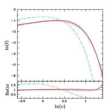
Figure 1: Multiplicity function at $t_{0}$ derived from the CUSP (red lines) and excursion set (green long-dashed line) formalisms, compared to Warren et al. (2006) analytic fit to the multiplicity function of simulated haloes (blue dotted line) over the maximum mass range $(2\times 10^{10}$ M_⊙, $2\times 10^{15}$ M_⊙) covered by simulations. For the CUSP case, we plot both the the approximate solution not accounting for the correlation between peaks of different scales (dashed line) and the more accurate solution given in Appendix (solid line). Ratios in the bottom panel are with respect to $f_{\rm W}$.

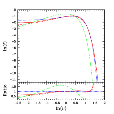
Figure 2: Same as Figure 1 but in a much wider mass range, corresponding to current haloes with masses from $1$ M_⊙ to $3\times 10^{16}$ M_⊙.

In Figure 1 we compare these two multiplicity functions at $t_{0}$ to the Warren et al. (2006) analytic expression, of the Sheth & Tormen (2002) form,

$$f_{\rm W}(\nu_{\rm es})=0.3303\left(\nu_{\rm es}^{1.625}+0.5558\right)\,{\rm e}^{-0.4565\nu_{\rm es}^{2}}\,,$$ (50)

fitting the multiplicity function of simulated haloes with FoF(0.2) masses at $t_{0}$ in all CDM cosmologies. $f_{\rm W}$ is usually expressed as a function of $\sigma_{0}^{\rm th}$ instead of $\nu_{\rm es}$; the expression (50) has been obtained from that usual expression assuming $\delta_{\rm c}(t_{0})=1.674$ (taking the value 1.686 would make no significant difference). In Figure 1, all the multiplicity functions are expressed as functions of the Gaussian height for ellipsoidal collapse and virialisation, $\nu$, instead of the top-hat height for spherical collapse, $\nu_{\rm es}$. The change of variable from $\nu_{\rm es}$ to $\nu$ has been carried out using the relation

$$\nu_{\rm es}=\frac{D(t)}{[a(t)]^{1.0628}}\,\nu\left\{1-0.0682\left[\frac{D(t)}{D(t_{0})}\right]^{2}\nu\right\}^{-1}$$ (51)

that follows from equations (34) and (36). This is a mere change of variable; it does not presume any modification in the assumptions entering the derivation of the different multiplicity functions.

As can be seen, while $f_{\rm es}$ shows significant deviations from $f_{\rm W}$ at both mass ends, $f_{\rm CUSP}$ is in excellent agreement with $f_{\rm W}$ all over the mass range covered by simulations. This is true regardless of whether we consider the approximate or more accurate versions of $f_{\rm CUSP}$. The deviation (of opposite sign in both cases) is less than 6.5%. We stress that there is no free parameter in the CUSP formalism, so this agreement is really remarkable.

It might be argued that $f_{\rm CUSP}$ cannot be trusted at small $\nu$’s because peaks with those heights have big chances to be destroyed by the gravitational tides of neighbouring massive peaks. Although this possibility exists, peaks suffering strong tides are expected to be nested within such neighbours and, hence, they should not be counted in the MF corrected for nesting. The correction for nesting becomes increasingly important, indeed, towards the small $\nu$ end. On the other hand, $f_{\rm CUSP}$ is well-normalised and still predicts the right abundance of massive haloes, which would hardly be the case if $f_{\rm CUSP}$ overestimated the abundance of low-mass objects. Therefore, we do not actually expect any major effect of that kind.

It is thus worth seeing how $f_{\rm CUSP}$ compares to $f_{\rm W}$ outside the mass range covered by simulations. In Figure 2 we represent the same multiplicity functions as in Figure 1 over a much wider range. Surprisingly, the agreement between $f_{\rm CUSP}$ and $f_{\rm W}$ is still very good. At very small $\nu$’s, $f_{\rm W}$ shows a slight trend to underestimate the abundance of haloes predicted by $f_{\rm CUSP}$, but the difference is small. It increases monotonously until reaching, in the case of the accurate version of $f_{\rm CUSP}$, a ratio of $\sim 0.70$ ($\sim 30$% deviation) at $M\sim 5\times 10^{4}$ M_⊙.

5.2 Approx Universality

The excursion set multiplicity function expressed as a function of $\nu_{\rm es}$, $f_{\rm es}(\nu_{\rm es})$, is cosmology-independent (it takes the same form [48] in all cosmologies) and time-invariant (the height is constant). Hence, it is universal in a strict sense. Such a universality is in fact what has motivated the use of the multiplicity function defined in equation (47) instead of the (non-universal) MF. Unfortunately, $f_{\rm es}$ does not properly recover the multiplicity function of simulated haloes.

But $f_{\rm CUSP}$ does, so the question rises: is $f_{\rm CUSP}$ also universal? Certainly, since the CUSP MF (as well as the real MF of simulated haloes) depends on the particular halo mass definition while $\sigma_{0}^{\rm th}$ does not, $f_{\rm CUSP}$ will necessarily depend (like the multiplicity function of simulated haloes; see e.g. Tinker et al. 2008) on the mass definition adopted. Thus, we will focus on the SO($\Delta_{\rm vir}$) or FoF(0.2) mass definitions, as suggested by the results of simulations (see the form [50] of $f_{\rm W}(\nu_{\rm es})$).

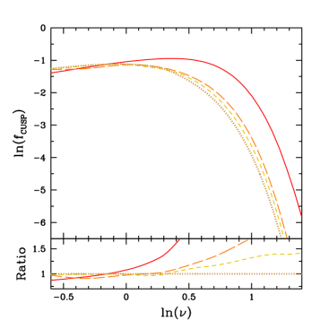
Figure 3: CUSP multiplicity functions at $z=0$, 5, 10 and 20, from left to right, in red (solid line), orange (long-dashed line), gold (dashed line) and brown (dotted line), respectively. Ratios in the bottom panel are with respect to the multiplicity function at $z=20$.

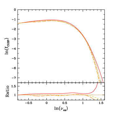
Figure 4: Same as Figure 3 but for $f_{\rm CUSP}$ expressed as a function of variable $\nu_{\rm es}$ instead of $\nu$. The green long-dashed line represents the multiplicity function that would be obtained from the excursion set formalism taking a density contrast for spherical collapse equal to 0.89 times the usual value.

By construction, the unconditioned and conditional peak number densities, $N(\sigma_{0},\delta_{\rm m})$ and $N(\sigma_{0},\delta_{\rm m}|\sigma_{0}^{\prime},\delta_{\rm m})$ entering the Volterra equation (16) take the same form of $\sigma_{0}$, $\sigma^{\prime}_{0}$ and $\delta_{\rm m0}$, through the heights $\nu$ and $\nu^{\prime}$, in all cosmologies (see eqs. [14], [17] and [15]). Certainly, these number densities also depend on $\gamma$, $\gamma^{\prime}$ and $R_{\star}$ that involve spectral moments of different orders and, hence, depend on the cosmology through the exact shape of the (linear) power spectrum. However, in all CDM cosmologies, the effective spectral index $n$ takes essentially the same fixed value, with less than 20% error over the whole mass range $(2\times 10^{10}$ M_⊙, $2\times 10^{15}$ M_⊙) of interest, implying that $\gamma\approx\gamma^{\prime}$ and $R_{\star}/{R_{\rm f}}[3(1-\gamma^{2})]^{1/2}$ takes almost “universal” values respectively equal to $0.6\pm 0.1$ and $1.4\pm 0.1$. Thus, those number densities are indeed very approximately universal functions of $\nu$ and $\nu^{\prime}$ but for a factor ${R_{\rm f}}^{-3}$. Moreover, if we multiply the Volterra equation (16) by $M/\bar{\rho}=4\pi\bar{\rho}_{\rm i}(q{R_{\rm f}})^{3}/(3\bar{\rho})$ so that its solution is directly $f_{\rm CUSP}$ (see eq. [49]), then the factor ${R_{\rm f}}^{-3}$ in the two number densities cancels with the factor ${R_{\rm f}}^{3}$ coming from the mass. Therefore, the solution $f_{\rm CUSP}$ of such a Volterra equation will have very approximately the same expression of $\nu$ in all CDM cosmologies, provided only the function $q(M,t)$ does.

But, according to equations (35)–(36) holding for SO($\Delta_{\rm vir}$) and FoF(0.19) haloes, $q(M,t)$ involves the ratio $\sigma^{\rm th}_{0}/\sigma_{0}$ which is not a function of $\nu$ alone, but also depends on $t$ through the cosmology-dependent ratio $D(t)/D(t_{0})$. Nevertheless, the term with the ratio $\sigma^{\rm th}_{0}/\sigma_{0}$ responsible of the undesired functionality of $q(M,t)$ is small in general (except for large $\nu$’s), particularly at high-$z$ where $D(t)/D(t_{0})$ becomes increasingly small. There, $q(M,t)$ becomes constant (equal to $Q^{-2/(n+3)}$) and $f_{\rm CUSP}(\nu)$ becomes essentially universal. However, at low-$z$ this is only true for small enough $\nu$’s.

In Figure 3 we show $f_{\rm CUSP}(\nu)$ in the concordant model for various redshifts (see JSDM for the corresponding MFs, in full agreement with the results of simulations). The deviations from universality or, more exactly, from time-invariance at high-$z$ are small as expected, but at low-$z$ they are very marked. Thus, $f_{\rm CUSP}(\nu)$ is far from universal (!).

But this result was not unexpected. Given the relation (51) between $\nu$ and $\nu_{\rm es}$, we cannot pretend that $f_{\rm CUSP}(\nu)$ is universal as a function of both arguments at the same time. Inspired by the universality of $f_{\rm es}(\nu_{\rm es})$, most efforts in the literature have been done in trying to find one mass definition rendering the multiplicity function of simulated haloes approximately universal as a function of the top-height for spherical collapse, not as a function of the (unknown) Gaussian height for ellipsoidal collapse and virialisation. Therefore, what we should actually check is whether $f_{\rm CUSP}$ is universal as a function of $\nu_{\rm es}$ and not of $\nu$. As shown in Figure 4, when the change of variable from $\nu$ to $\nu_{\rm es}$ is made, $f_{\rm CUSP}$ becomes indeed almost fully time-invariant. Strictly, it still shows slight deviations from universality at large $\nu_{\rm es}$, but these deviations are in full agreement with those found in simulations (see Fig. 14 in Lukić et al. 2007).

Thanks to the CUSP formalism, we can determine the Gaussian height for ellipsoidal collapse and virialisation corresponding to any desired mass definition. Thus, we can seek the halo mass definition for which $f_{\rm CUSP}$ expressed as a function of $\nu$ takes a universal form. According to the reasoning above, for this to be possible the ratio $\sigma_{0}^{\rm th}/\sigma_{0}$ should be equal to $1+c\,\nu$, with $c$ equal to an arbitrary universal constant. This would ensure both that the partial derivative of $n_{\rm CUSP}$ with respect to $\sigma_{0}$ coincides with the partial derivative with respect to $\sigma_{0}^{\rm th}$ and that the function $q(M,t)$ is a function of $\nu$ alone: $q(\nu)\approx[Q\,\left(1+c\,\nu\right)]^{-2/(n+3)}$. Consequently, following the procedure given in Section 3.2, we can infer, from such a function $q(\nu)$ and any arbitrary function $\delta_{\rm m}(t)$, the desired halo mass definition. Unfortunately, despite the freedom left in those two functions, the mass definition so obtained will hardly coincide with any of the practical SO and FoF ones. Thus, it is actually preferable to keep on requiring the universality of the multiplicity function in terms of $\nu_{\rm es}$ as usual.

But this does not explain why the FoF mass definition with linking length $\sim 0.2$ is successful in giving rise to a universal multiplicity function expressed as a function of $\nu_{\rm es}$. Clearly, what makes this mass definition special is that, for the reasons explained in Section 4, it coincides with the SO($\Delta_{\rm vir}$) definition. In fact, as mentioned there, the exact value of the linking length may somewhat vary with time and cosmology, so the canonical mass definition would be the SO($\Delta_{\rm vir}$) definition rather than the FoF(0.2) one. But why should a mass definition that involves the virial overdensity $\Delta_{\rm vir}$ arising from the formal spherical top-hat model successfully lead to a universal multiplicity function expressed as a function of $\nu_{\rm es}$ if haloes actually form from peaks that undergo ellipsoidal collapse and virialisation? The reason for this is that, as a consequence of the inside-out growth of haloes formed from ellipsoidal collapse and virialisation, they satisfy the relation (25), identical to the relation (21) satisfied by objects formed in the spherical top-hat model.

As mentioned, an interesting consequence of this “coincidence” is that the top-hat density contrast for ellipsoidal collapse and virialisation for SO($\Delta_{\rm vir}$) masses, $\delta_{\rm m}^{\rm th}$, takes a universal value, independent of $M$, approximately equal to 0.9 times the top-hat density contrast for spherical collapse, $\delta_{\rm c}(t)$. Given this relation, changing the latter density contrast by the former in the excursion set formalism, $f_{\rm es}(\nu_{\rm es})$ should keep on being universal and, in addition, recover the real multiplicity function of haloes formed by ellipsoidal collapse and virialisation. As shown in Figure 5, this is fully confirmed. One must just renormalise the resulting modified excursion set multiplicity function in the relevant mass range by multiplying it by 0.714. But this is simply due to the fact that the correction for nesting achieved in the excursion set formalism is inconsistent with top-hat smoothing, which yields an increasing deviation of the predicted function at low-masses, the most affected by such a correction. (The right normalisation should naturally result if we could implement the excursion set correction for nesting with top-hat smoothing.)

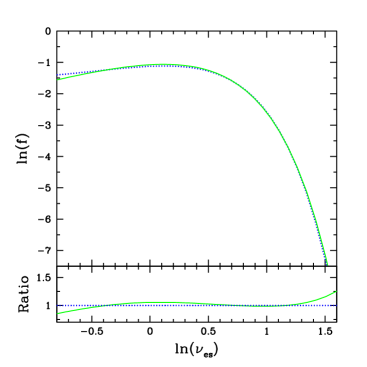
Figure 5: Modified excursion set multiplicity function resulting from a density contrast for collapse equal to 0.889 times the usual value (solid green line), compared to $f_{\rm W}$ for FoF(0.2) haloes (dotted blue line). Both multiplicity functions are strictly universal, so the two curves hold for any arbitrary redshift.

Therefore, the ultimate reason for the success of the SO($\Delta_{\rm vir}$) mass definition, and by extension of the FoF(0.2) one, is that, as a consequence of the inside-out-growth of accreting haloes, the corresponding top-hat density contrast for ellipsoidal collapse and virialisation is essentially proportional to the formal top-hat density contrast for spherical collapse.

To end up we want to mention that the previous result suggests what is actually the most natural argument for the halo multiplicity function to take a universal form: the top-hat height for ellipsoidal collapse and virialisation, $\nu^{\rm th}$, defined as $\delta_{\rm m0}^{\rm th}(t_{0})/\sigma^{\rm th}_{0}\approx 0.889\,\delta_{\rm c0}(t_{0})/\sigma^{\rm th}_{0}$. This expression holds for the current time and the concordant cosmology. The exact dependence of $\delta_{\rm m}^{\rm th}(t)$ (or, more exactly, of the ratio $\delta_{\rm m}^{\rm th}(t)/\delta_{\rm c}(t)$) on time and cosmology is hard to tell owing to the insufficient precision of the inverse Laplace transform of equation (31) or, alternatively, the unknown range of $c$ values of simulated haloes with SO($\Delta_{\rm vir}$) masses at other times and cosmologies. But a reasonable guess is that such a dependence should make $f_{\rm CUSP}(\nu^{\rm th})$ be strictly universal and equal to the multiplicity function represented in Figure 6. The reason for this guess is the full consistency, at any time and cosmology, between the SO($\Delta_{\rm vir}$) mass definition and the real dynamics of collapse and virialisation of halo seeds. A similar full consistency is what causes $f_{\rm es}(\nu_{\rm es})$ to be also strictly universal. The difference between the two cases is that, while the excursion set formalism assumes a non-realistic dynamics of collapse (unless it is modified as prescribed above), the CUSP formalism assumes the right dynamics.

Figure 6: Same as Figures 3 and 4 but for $f_{\rm CUSP}$ expressed as a function of the top-hat height for ellipsoidal collapse and virialisation, $\nu^{\rm th}$, as suggested by the CUSP formalism. This multiplicity function would be strictly universal, so the curves for the different redshifts fully overlap. For comparison we also plot the function $f_{\rm W}$ (blue dotted curve) expressed with the same argument.

6 Discussion and Conclusions

To have a fully satisfactory understanding of the role of the halo mass definition in the properties of the halo multiplicity function we must still answer one last question: why is the simplifying assumption that “haloes form by pure accretion” used in all the derivations of the halo MF so successful? As discussed in SVMS, major mergers go unnoticed, indeed, in the typical spherically averaged density profile and abundance of virialised haloes because the virialisation taking place in such dramatic events is a real relaxation causing the memory loss of the halo past history. In other words, virialised haloes do not know whether they have suffered major mergers or they have formed by pure accretion. As a consequence, to derive the halo MF (as well as any other typical halo property, except those arising from two-body relaxation) one has the right to assume, with no loss of generality, that all haloes form by pure accretion. Note that, on the contrary, the virialisation produced in smooth accretion is not a full relaxation: the absence of apocentre-crossing during such a virialisation (SVMS) preserves some memory of the initial seed. This is the reason why the density profile for individual haloes can be inferred from the respective peak trajectories $\delta(R)$ or, equivalently, from their accretion history. The fact that the density profile of accreting haloes remembers their mass aggregation history is at the base of the well-known assembly bias.

JSDM showed that the typical spherically averaged density profile and MF of haloes derived in the framework of the CUSP formalism recover the results of numerical simulations for haloes for any chosen mass definition. In the present paper, we have seen that the SO($\Delta_{\rm vir}$) and FoF(0.2) mass definitions are essentially equivalent to each other and their respective multiplicity functions expressed as a function of the top-hat height for spherical collapse are very similar and approximately universal. The reason for those trends is that, as a consequence of the inside-out growth of accreting haloes, the top-hat density contrast for ellipsoidal collapse for those particular mass definitions is essentially universal and equal to $\sim 0.9$ times the usual top-hat density contrast for spherical collapse.

ACKNOWLEDGEMENTS

This work was supported by the Spanish DGES AYA2009-12792-C03-01 and AYA2012-39168-C03-02 and the Catalan DIUE 2009SGR00217. One of us, EJ, was beneficiary of the grant BES-2010-035483.

Appendix A Accurate Conditional Peak Number Density

As shown in Manrique et al. (1998), the conditional number density $N^{\rm nn}(\sigma_{0},\delta_{\rm m}|\sigma^{\prime}_{0},\delta_{\rm m})$ of peaks with $\delta_{\rm m}$ per infinitesimal $\ln\sigma_{0}^{-1}$ subject to being located in the collapsing cloud of non-nested peaks with $\delta_{\rm m}$ at $\sigma^{\prime}_{0}<\sigma_{0}$ is well-approximated by the integral over the distance $r$ from the background peak out to the radius $R_{\rm p}$ of the collapsing cloud in units of $q(M,t){R_{\rm f}}$ of the conditional number density of peaks with $\delta_{\rm m}$ per infinitesimal $\ln\sigma_{0}^{-1}$, subject to being located at a distance $r$ from a background peak, $N(\sigma_{0},\delta_{\rm m}|\sigma^{\prime}_{0},\delta_{\rm m},r)$,

$$N^{\rm nn}(\sigma_{0},\delta_{\rm m}|\sigma^{\prime}_{0},\delta_{\rm m})=\!C\!\!\int_{0}^{1}\!\!{\rm d}r\,3r^{2}N(\sigma_{0},\delta_{\rm m}|\sigma_{0},\delta_{\rm m},r)\,.$$ (52)

The conditional number density in the integrant on the right of equation (52) can be obtained, as the ordinary number density (14), from the conditional density of peaks per infinitesimal $x$ and $\nu$, subject to being located at the distance $r$ from a background peak with $\nu$ at $\sigma^{\prime}_{0}$, calculated by BBKS. The result is (Manrique et al., 1998)

$$\,N(\sigma_{0},\delta_{\rm m}|\sigma^{\prime}_{0},\delta_{\rm m},r){\rm d}\ln\sigma_{0}^{-1}~{}~{}~{}~{}~{}~{}~{}~{}~{}~{}~{}~{}~{}~{}~{}~{}~{}~{}~{}~{}~{}~{}$$

$$=\frac{\langle x\rangle[\tilde{\sigma}_{0}(r),\delta_{\rm m}]}{(2\pi)^{2}\,R_{\star}^{3}\,\gamma\,e(r)}{\rm e}^{-\frac{\left[\nu-\epsilon(r)\,\nu^{\prime}(r)\right]^{2}}{2e^{2}(r)}}{\rm d}\ln\sigma_{0}^{-1}\,,$$ (53)

where $\langle x\rangle[\tilde{\sigma}_{0}(r),\delta_{\rm m}]$ is the average curvature of peaks with $\delta_{\rm m}$ at $\sigma_{0}$ located at a distance $r$ from a background peak with identical density contrast at $\sigma^{\prime}_{0}$. This latter function takes just the same form as the usual average curvature $\langle x\rangle(\sigma_{0},\delta_{\rm m})$ for the properly normalised (by integration over $x$ from zero to infinity) curvature distribution function

$$h(x,\sigma_{0},\delta_{\rm m})=f(x)\,{\rm e}^{-{(x-x_{\star})^{2}\over 2(1-\tilde{\gamma}^{2})}},$$ (54)

$$f(x)=\frac{x^{3}-3x}{2}\left\{{\rm erf}\!\left[\left(\frac{5}{2}\right)^{1/2}x\right]+{\rm erf}\!\left[\left(\frac{5}{2}\right)^{1/2}\frac{x}{2}\right]\right\}$$

$$+\left(\frac{2}{5\pi}\right)^{\!\!1/2}\!\!\left[\left(\!\frac{31x^{2}}{4}+\frac{8}{5}\!\right){\rm e}^{-\frac{5x^{2}}{8}}+\left(\!\frac{x^{2}}{2}-\frac{8}{5}\!\right){\rm e}^{-\frac{5x^{2}}{2}}\right]\!,$$ (55)

but for $\tilde{x}_{\star}(r)\equiv\tilde{\gamma}(r)\,\tilde{\nu}(r)$ instead of $x_{\star}\equiv\gamma\,\nu$, being

$$\tilde{\gamma}^{2}(r)=\gamma^{2}\left[1+\epsilon(r)^{2}\,{(1-r_{1})^{2}\over 1-\epsilon(r)^{2}}\right]$$ (56)

$$\tilde{\nu}(r)\!=\!{\gamma\over\tilde{\gamma}(r)}\,{1-r_{1}\over 1-\epsilon(r)^{2}}\left[\nu\!\left({1-\epsilon(r)^{2}r_{1}\over 1-r_{1}}\!\right)\!-\epsilon(r)\nu^{\prime}(r)\right]\!.$$ (57)

In equations (53), (56) and (57), we have used the following notation: $e(r)=\sqrt{1-\epsilon(r)^{2}}$, $\epsilon(r)=(\sigma_{0}^{2}(R_{\rm h})$ $/[\sigma_{0}\sigma^{\prime}_{0}]g(r,\sigma^{\prime}_{0})$, and $\nu^{\prime}(r)=g(r,\sigma^{\prime}_{0})\overline{\delta(r)}/\sigma^{\prime}_{0}$ and $r_{1}=[\sigma_{0}({R_{\rm f}})\sigma_{1}(R_{\rm h})/(\sigma_{1}({R_{\rm f}})\sigma_{0}(R_{\rm h}))]^{2}$, where $R_{\rm h}$ is defined as usual and $g(r,\sigma^{\prime}_{0})$ is $\left\{1-[\Delta\delta^{\prime}(r)]^{2}/\sigma^{\prime}_{0}\right\}^{1/2}$, being $\overline{\delta^{\prime}(r)}$ and $\Delta\delta^{\prime}(r)$ the mean and rms density contrasts at $r$ from the background peak, respectively given by

$$\overline{\delta(r)}=\frac{\gamma\delta_{\rm mi}}{1-\gamma^{2}}\left(\frac{\psi}{\gamma}+\frac{\nabla^{2}\psi}{u^{2}}\right)-\frac{x\sigma_{0}}{1-\gamma^{2}}\left(\gamma\psi+\frac{\nabla^{2}\psi}{u^{2}}\right)$$ (58)

$$[\Delta\delta(r)]^{2}=\sigma_{0}^{2}\bigg{\{}\!1\!-\!\frac{1}{1-\gamma^{2}}\left[\psi^{2}+\!\!\left(2\gamma\psi+\frac{\nabla^{2}\psi}{u^{2}}\!\!\right)\frac{\nabla^{2}\psi}{u^{2}}\right]$$

$$-5\left(\frac{3\psi^{\prime}}{u^{2}r}-\frac{\nabla^{2}\psi}{u^{2}}\right)^{2}-\frac{3(\psi^{\prime})^{2}}{\gamma u^{2}}\bigg{\}}\,,~{}~{}~{}~{}~{}~{}~{}~{}~{}~{}~{}~{}~{}~{}~{}~{}~{}~{}~{}~{}$$ (59)

where $\xi(r)$ is the mass correlation function at the separation $r$ and scale ${R_{\rm f}}$, $\psi$ is the ratio $\xi(r)/\xi(0)$, $\psi^{\prime}$ is its $r$-derivative and $u$ is defined as $[q(M,t){R_{\rm f}}]^{2}\sigma_{2}({R_{\rm f}})/\sigma_{0}({R_{\rm f}})$. Lastly, the factor $C$ on the right, defined as

$$C\equiv\frac{4\pi s^{3}N(\sigma^{\prime}_{0},\delta_{\rm m})}{3N(\sigma_{0},\delta_{\rm m})}\int_{0}^{s}{\rm d}r\,3r^{2}\,N(\sigma_{0},\delta_{\rm m}|\sigma^{\prime}_{0},\delta_{\rm m},r)\,$$ (60)

with $s$ equal to the mean separation between the larger scale non-nested peaks drawn from their mean number density, is to correct for the overcounting of background peaks in $N(\sigma_{0},\delta_{\rm m}|\sigma^{\prime}_{0},\delta_{\rm m},r)$ as they are not explicitly required to be non-nested.

The simpler version of the conditional peak number density given in Section 2.2 can be readily recovered from the present one by ignoring the radial dependence of the typical spherically averaged density profile around peaks, that is taking $\overline{\delta(r)}=\delta_{\rm m}$ and $\Delta\delta(r)=0$.

References

- Appel & Jones (1990) Appel L. & Jones B. J. T., 1990, MNRAS, 245, 522
- Bardeen et al. (1986) Bardeen J. M., Bond J. R., Kaiser N., Szalay A. S., 1986, ApJ, 304, 15 (BBKS)
- Bond (1988) Bond J. R. in Unrhu W. G., Semenov W. G., eds., The Early Universe, Reidel, Dordrecht, p. 283
- Bond et al. (1991) Bond J. R., Cole S., Efstathiou G., Kaiser N., 1991, ApJ, 379, 440
- Bond & Myers (1996) Bond, J. R. & Myers S. T., 1996, ApJS, 103, 41
- Bond (1989) Bond, J. R., 1989, in Frontiers in Physics: From Colliders to Cosmology, ed. A. Astbury, B. A. Campbell, W. Israel, F. C. Khana (Singapore: World Scientific), p. 182
- Colafrancesco et al. (1989) Colafrancesco S., Lucchin F., Matarrese S., 1989, ApJ, 345, 3
- Cole & Lacey (1996) Cole S. & Lacey C., 1996, MNRAS, 281, 716
- Courtin et al. (2011) Courtin J., Rasera Y., Alimi, J. M., Corasaniti P. S., Boucher V., Füzfa A., MNRAS, 410, 1911
- Crocce et al. (2010) Crocce M., Fosalba P., Castander F. J., Gaztañaga E., 2010, MNRAS, 403, 1353
- Davis et al. (1985) Davis M., Efstathiou G., Frenk C. S., White S. D. M., ApJ, 292, 371
- Despali et al. (2013) Despali G., Tormen G., Sheth R. K., 2013, MNRAS, 431, 1143
- Efstathiou et al. (1988) Efstathiou G., Frenk C. S., White S. D. M., Davis M., MNRAS, 235, 715
- Elia et al. (2012) Elia A., Ludlow A. D., Porciani C., 2012, MNRAS, 421, 3472
- Epstein (1983) Epstein R. I., 1983, MNRAS, 205, 207
- Frenk et al. (1988) Frenk C. S., White S. D. M., Davis M., Efstathiou G., 1988, ApJ, 327, 507
- Gelb & Bertschinger (1994) Gelb J. & Bertschinger E., 1994, ApJ, 436, 467
- Gross et al. (1998) Gross M. A. K., Somerville R. S., Primack J. R., Holtzman J., Klypin A., 1998, MNRAS, 301, 81
- Hanami (2001) Hanami H., 2001, MNRAS, 327, 721
- Hahn & Paranjape (2013) Hahn O., & Paranjape A., 2013, arXiv:1308.4142
- Heitmann et al. (2006) Heitmann K., Lukić Z., Habib S., Ricker P. M., 2006, ApJ, 642, L85
- Henry (2000) Henry, J. P., 2000, ApJ, 534, 565
- Jenkins et al. (2000) Jenkins A., Frenk C. S., White S. D. M., et al., 2001, MNRAS, 321, 372
- Jenkins et al. (2001) Jenkins A., Frenk C. S., White S. D. M., et al., 2001, MNRAS, 321, 372
- Juan et al. (2013) Juan E., Salvador-Solé E., Domènech G., Manrique A., 2013, submitted to MNRAS(JSDM)
- Knebe et al. (2011) Knebe A., Knollmann S. R., Muldrew S. I., et al., 2011, MNRAS, 415, 2293
- Lacey & Cole (1994) Lacey C. & Cole S., 1994, MNRAS, 271, 671
- Lee & Shandarin (1998) Lee J. & Shandarin S. F., 1998, ApJ, 500, 14
- Lukić et al. (2007) Lukić Z., Heitmann K., Habib S., Bashinsky, S., Ricker P., ApJ, 671, 1160
- Maggiore & Riotto (2010) Maggiore M. & Riotto A., 2010, ApJ, 717, 515
- Manrique & Salvador-Solé (1995) Manrique A. & Salvador-Solé E., 1995, ApJ, 453, 6 (MSS)
- Manrique et al. (1998) Manrique A., Raig A., Solanes J. M., González-Casado G., Stein, P., Salvador-Solé E., 1998, ApJ, 499, 548
- Monaco (1995) Monaco P., 1995, ApJ, 447, 23
- More et al. (2011) More S., Kratsov A., Dalal N., Gottlöber S., 2011, ApJS, 195, 1
- Musso et al. (2012) Musso M., Paranjape A., Sheth R. K., 2012, MNRAS, 427, 3145
- Musso & Paranjape (2012) Musso M. & Paranjape A., 2013, MNRAS, 420, 369.
- Navarro et al. (1997) Navarro J. F., Frenk C. S. & White S. D. M., 1997, ApJ, 490, 493
- Paranjape & Sheth (2012) Paranjape A. & Sheth R. K., 2012, MNRAS, 426, 2789
- Paranjape et al. (2012) Paranjape A., Lam T. Y., & Sheth R. K., 2012, MNRAS, 420, 1429
- Paranjape et al. (2013) Paranjape A., Sheth R. K., Desjacques V., 2013, MNRAS, 431, 1503
- Planck Collaboration et al. (2013) Planck Collaboration, Ade, P. A. R., Aghanim, N., et al. 2013, arXiv:1303.5076
- Peacock & Heavens (1985) Peacock, J. A. & Heavens A. F., 1985, MNRAS, 217, 805
- Peacock & Heavens (1990) Peacock, J. A. & Heavens A. F., 1990, MNRAS, 243, 133
- Peebles (1980) Peebles, P. J. E., The Large-Scale Structure of the Universe, Princeton Univ. Press (1980)
- Press & Schechter (1974) Press W. H. & Schechter P., 1974, ApJ, 187, 425
- Reed et al. (2003) Reed D., Gardner J., Quinn T., et al., 2003, MNRAS, 346, 565
- Robertson et al. (2009) Robertson B. E., Kravtsov A. V., Tinker J., Zentner A. R., 2009, ApJ, 696, 636
- Salvador-Solé et al. (2012) Salvador-Solé E., Viñas J., Manrique A., Serra S., 2012, MNRAS, 423, 2190 (SVMS)
- Sheth & Tormen (2002) Sheth R. K. & Tormen G., 2002, MNRAS, 329, 61
- Sugiyama (1995) Sugiyama, N. 1995, ApJS, 100, 281
- Tinker et al. (2008) Tinker J., Kravtsov A. V., Klypin A., Abazajian K., Warren M., Yepes G., Gottlöber S., Holz ED. E., 2008, ApJ, 688, 709
- Warren et al. (2006) Warren M. S., Abazajian K., Holz D. E., Teodoro L., 2006, ApJ646, 881
- White (2002) White M., ApJS, 2002, 143, 241
- White et al. (1993) White S. D. M., Efstathiou G., Frenk C. S., 1993, MNRAS, 262, 1023
- White (2001) White M., 2001, A&A, 367, 27
- White (2002) White M., 2002, ApJS, 143, 241
- Zhao et al. (2009) Zhao, D. H., Jing, Y. P., Mo, H. J., Börner, G. 2009, ApJ, 707, 354