Fixing a Rigorous Formalism for the Accurate Analytic Derivation of Halo Properties

Abstract

We establish a one-to-one correspondence between virialised haloes and their seeds, namely peaks with a given density contrast at appropriate Gaussian-filtering radii, in the initial Gaussian random density field. This fixes a rigorous formalism for the analytic derivation of halo properties from the linear power spectrum of density perturbations in any hierarchical cosmology. The typical spherically averaged density profile and mass function of haloes so obtained match those found in numerical simulations.

1 INTRODUCTION

In the lack of an exact treatment of non-linear structure evolution, most research in the field of dark matter clustering has been conducted through $N$-body simulations (Frenk & White, 2012)).

The main difficulty in the analytic derivation of halo properties comes from the effects of major mergers. For this reason, all efforts have focused on haloes formed by monolithic collapse or pure accretion. Nevertheless, as far as virialisation is a real relaxation, the properties of virialised haloes cannot depend on whether or not they have suffered major mergers (Salvador-Solé et al. 2012a, hereafter SVMS).

Following the seminal work by Gunn & Gott (1972), various authors tried to infer the density profile for haloes emerging by pure accretion from linear perturbations in the density field at a small cosmic time $t_{\rm i}$, assuming spherical collapse and self-similarity (see references in SVMS). A big step forward was taken when halo seeds were identified as density maxima (peaks) in the initial Gaussian random field (Doroshkevich 1970; Bardeen et al. 1986, hereafter BBKS). This led to typical density profiles in fair agreement with the results of numerical simulations (Avila-Reese et al. 1998; Del Popolo et al. 2000; Ascasibar et al. 2004). Those solutions were however not yet fully satisfactory because the typical peak density profile derived by BBKS is convolved with a Gaussian window and peaks are triaxial and undergo ellipsoidal collapse. On the other hand, the effects of shell-crossing during virialisation were not accurately treated.

Other authors concentrated in the halo mass function (MF). Press & Schechter (1974) derived it assuming that the seeds of haloes with mass $M$ at the time $t$ are overdense regions in the Gaussian random density field at $t_{\rm i}$ that, smoothed with a top-hat filter at the scale $M$, have density contrast $\delta$ equal to the critical value $\delta_{\rm c}(t)$ for spherical collapse at $t$. The MF so obtained was similar to that found in simulations except for a factor two. Bond et al. (1991) corrected this flaw using the excursion set formalism dealing with the $\delta(M)$ trajectories traced by fixed points in the initial density field filtered by a sharp k-space window of varying scale in the presence of an absorbing barrier at $\delta_{\rm c}(t)$ (see also Sheth & Tormen 2002 and Maggiore & Riotto 2010). Bond (1988), Colafrancesco et al. (1989), Peacock & Heavens (1990), Appel & Jones (1990), Bond & Myers (1991) and Paranjape & Sheth (2012) extended this approach to peaks and Manrique & Salvador-Solé (1995, hereafter MSS) and Manrique et al. (1998) developed the ‘ConflUent System of Peak trajectories’ (CUSP) formalism leading to a fully consistent analytic derivation of the halo MF from the number density of non-nested peaks (see also Hanami 2001).

The CUSP formalism follows from the peak Ansatz inspired by the spherical collapse that there is a one-to-one correspondence between virialised haloes with mass $M$ at $t$ and non-nested peaks with density contrast $\delta(t)$ at the filtering radius $R(M)$. Unfortunately, these two functions were determined by fitting the halo MF, which caused the formalism to loose its predicting power. On the other hand, the validity of the peak Ansatz was not proved.

Notwithstanding, this formalism has recently acquired a renewed interest. As shown by SVMS, it allows one to find the unconvolved density profile of peaks. Then, taking into account that accreting haloes develop from the inside out, one can exactly account for the effects of ellipsoidal collapse and shell-crossing and infer the typical spherically averaged halo density profile. The used of the approximated functions $\delta(t)$ and $R(M)$ obtained by MSS could explain the small departures found in the predicted density profiles from those found in simulations.

In the present Letter, we justify and accurately fix the halo-peak correspondence and re-derive the halo density profile and MF. We use the concordant $\Lambda$CDM cosmology with $\Omega_{\Lambda}=0.73$, $\Omega_{\rm m}=0.23$, $\Omega_{\rm b}=0.045$, $H_{0}=0.71$ km s^-1 Mpc^-1, $\sigma_{8}=0.81$ and $n_{\rm s}=1$ together with the BBKS CDM spectrum with Sugiyama (1995) shape parameter.

2 The CUSP Formalism

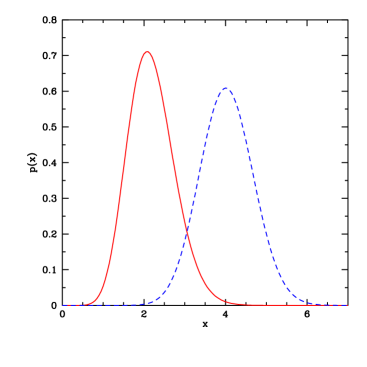
Figure 1: Distribution of curvatures for peaks corresponding to current haloes with extreme SO ($\Delta_{\rm vir}$) masses of $10^{8}$ M_⊙ (red solid line) and $10^{16}$ M_⊙ (blue dashed line), for which $\langle(x-\langle x\rangle)^{2}\rangle^{1/2}/\langle x\rangle$ are respectively equal to 0.25 and 0.16.

Simulations show that virialised haloes form from peaks. Only $15-20$ % of haloes arise from two nodes (Porciani et al., 2002; Ludlow & Porciani, 2011), which is compatible with them being currently undergoing a major merger. In fact, Hahn & Paranjape (2013) found that all virialised haloes arise from peaks. However, the one-to-one correspondence between haloes with $M$ at $t$ and peaks at $t_{\rm i}$ with density contrast dependent only on $t$ as stated in the peak Ansatz seems to be at odds with the idea that the time of ellipsoidal collapse of peaks depends not only on their density contrast $\delta$ but also on their ellipticity and density slope.

But the scatters in ellipticity and in density slope of peaks with given $\delta$ and $R$ are small compared to the mean values. This can be seen indeed from the distribution of peak ellipticities (BBKS) and the result below that the unconvolved density contrast profile $\delta_{\rm p}(r)$ of halo seeds is the inverse Laplace transform of the trajectory $\delta(R)$ they follow when filtered with a Gaussian filter of varying radius (see eq. [11]). The density slope of seeds, ${\rm d}\delta_{\rm p}/{\rm d}r$, is then proportional to the slope ${\rm d}\delta/{\rm d}R$ of the peak trajectory,

$$\frac{\partial\delta}{\partial R}=R\,\nabla^{2}\delta\equiv-x\,\sigma_{2}(R)\,R\,,$$ (1)

where $x$ is the peak curvature, that is minus the Laplacian scaled to the mean value, equal to the second order spectral moment $\sigma_{2}$. As the Laplace transform is linear, we then have (see Fig. 1)

$$\frac{\big{\langle}\big{(}\frac{{\rm d}\rho_{\rm p}}{{\rm d}r}-\big{\langle}\frac{{\rm d}\rho_{\rm p}}{{\rm d}r}\big{\rangle}\big{)}^{2}\big{\rangle}^{1/2}}{\big{\langle}\frac{{\rm d}\rho_{\rm p}}{{\rm d}r}\big{\rangle}}\approx\frac{\langle(x-\langle x\rangle)^{2}\rangle^{1/2}}{\langle x\rangle}\ll 1\,.$$ (2)

Thus, if we are interested in the typical properties of haloes, we can safely assume peaks at $t_{\rm i}$ with $\delta$ at $R$ having the same typical ellipticity and density slope. Then, the mass $M$ of virialised haloes arising at any $t$ from peaks with a fixed value of $\delta=\delta_{\rm mi}$ is a function of $R$ alone. And, adopting the halo mass definition that exactly matches the function $M(R)$, we end up with the following one-to-one correspondence between haloes with $M$ at $t$ and non-nested peaks at $t_{\rm i}$ with density contrast $\delta_{\rm mi}$ at Gaussian-filtering radii ${R_{\rm f}}$,

$$\delta_{\rm mi}(t)=\delta_{\rm m}(t)\frac{D(t_{\rm i})}{D(t)}\,,$$ (3)

$${R_{\rm f}}(M,t)=\frac{1}{q(M,t)}\left[\frac{3M}{4\pi\bar{\rho}(t_{\rm i})}\right]^{1/3}\,,$$ (4)

where $\bar{\rho}_{\rm i}$ is the mean cosmic density at $t_{\rm i}$ and $D(t)$ is the cosmic growth factor.

The dependence on $t_{\rm i}$ on the right of equations (3)–(4) ensures the arbitrariness of that initial time. Equation (3) defines the density contrast $\delta_{\rm m}(t)$ of peaks with $\delta_{\rm mi}(t)$ at $t_{\rm i}$ linearly extrapolated to the time $t$, and equation (4) defines the radius $q(M,t)$ of halo seeds in units of the radius ${R_{\rm f}}$ of the Gaussian filter. As shown by several authors (e.g. Hahn & Paranjape 2013), the density contrast of density perturbations undergoing ellipsoidal collapse depends on $M$, while in the CUSP formalism it does not. We note however that in all those works the filter used is top-hat, while in the CUSP formalism it is Gaussian. This introduces a freedom in ${R_{\rm f}}$ associated to a given halo mass $M$ through the function $q(M,t)$. We can then chose $\delta_{\rm mi}(t)$ independent of $M$ and let the radius of the seed in units of ${R_{\rm f}}$ to depend on $M$.

The use of a Gaussian filter is indeed mandatory for the density contrast of peaks (with negative values of $\nabla^{2}\delta$) to be always decreasing with increasing filtering radius (see eq. [1]), for consistency with the ever increasing mass of haloes, where $\delta_{\rm mi}(t)$ is a decreasing function of $t$ and ${R_{\rm f}}(M,t)$ an increasing function of $M$. Besides these restrictions, the functions $\delta_{\rm mi}(t)$ and ${R_{\rm f}}(M,t)$ or, equivalently, $\delta_{\rm m}(t)$ and $q(M,t)$ are arbitrary and fix one specific halo mass definition each. Certainly, the mass definition corresponding to any given couple of functions $\delta_{\rm m}(t)$ and $q(M,t)$ is very hard to infer and will anyway differ from any usual one, in general. But, as shown below, we can proceed the other way around: exactly determine the functions $\delta_{\rm m}(t)$ and $q(M,t)$ that correspond to any desired mass definition.

3 Fixing the halo-peak correspondence

The so-called spherical overdensity (SO) and friends-of-friends (FoF) mass definitions are the most popular ones. In the former, mostly used in observational works and numerical studies of the spherically averaged halo density profile, $\rho_{\rm h}(r)$, the mass of a halo is that inside the radius $R_{\rm h}$ defining an inner mean density $\bar{\rho}_{\rm h}(R_{\rm h})$ equal to a fixed overdensity $\Delta$ times the mean cosmic density,

$$\bar{\rho}_{\rm h}(R_{\rm h})=\Delta\bar{\rho}(t)\,.$$ (5)

$\Delta$ is often taken equal to the cosmology- and time-dependent virial value $\Delta_{\rm vir}(t)$ arising from the top-hat spherical collapse model. This mass definition is from now on referred to as SO($\Delta_{\rm vir}$).

But in numerical studies of the MF, the mass of a halo is usually taken equal to the total mass of its particle members, identified by means of a FoF percolation finder, with fixed linking length $b$, in units of the mean interparticle separation. This coincides with the mass inside the radius $R_{\rm h}$ where spheres of radius $b$ harbour two particles in average (Lacey & Cole, 1994)

$$\rho_{\rm h}(R_{\rm h})=\frac{3}{2\pi}\,b^{-3}\bar{\rho}(t)\,.$$ (6)

$b$ is usually taken equal to 0.2 leading to a roughly universal MF. Such a mass is from now on referred to as FoF(0.2).

In the present Letter, we consider both mass definitions, SO($\Delta_{\rm vir}$) and FoF(0.2). This facilitates the comparison with the results of numerical simulations regarding either the halo density profile or the MF and illustrates the possibility to apply the same procedure to any desired mass definition.

3.1 Spherically Averaged Halo Density Profile

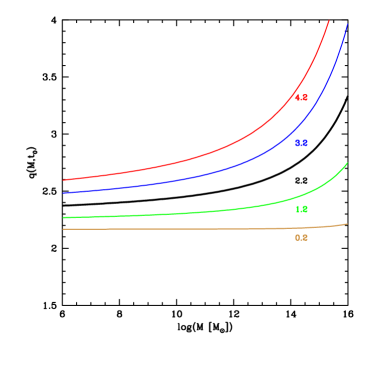
Figure 2: Radius of seeds, in units of Gaussian filtering radius, of present haloes with SO($\Delta_{\rm vir}$) masses (solid lines) and FoF(0.19) masses (dashed lines) for the quoted values of $\delta_{\rm m}(t_{0})$. The two kinds of curves fully overlap, but this is not the case for any arbitrary mass definition. The thick black line is for the value of $\delta_{\rm m}(t_{0})$ yielding the right normalisation of the associated MF.

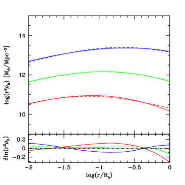
Figure 3: Typical spherically averaged density profiles (solid lines) predicted for current haloes with SO($\Delta_{\rm vir}$) masses equal to $5\times 10^{10}$ M_⊙ (red), $5\times 10^{12}$ M_⊙ (green) and $5\times 10^{14}$ M_⊙ (blue), compared to the typical NFW profiles of simulated haloes (dashed lines) with identical masses and the same cosmology according to Zhao et al. (2009).

As shown in SVMS, during the virialisation of a triaxial halo, shells cross each other without the crossing of their respective apocentres. As a consequence, virialised haloes develop from the inside out, keeping their instantaneous inner structure unaltered. Then, the radius $r$ encompassing the mass $M$ exactly satisfies the relation

$$r=-\frac{3GM^{2}}{10E_{\rm p}(M)}\,,$$ (7)

where $E_{\rm p}(M)$ is the (non-conserved) total energy of the spherically averaged seed of the halo progenitor with mass $M$. Therefore, provided $E_{\rm p}(M)$ is known, the relation (7) can be used to infer the mass profile $M(r)$ and, by differentiation, the spherically averaged density profile $\rho_{\rm h}(r)$ of the final halo.

The energy distribution $E_{\rm p}(M)$ of the protohalo is given, in the parametric form, by

$$E_{\rm p}(r)=4\pi\!\int_{0}^{r}\!\!{\rm d}\tilde{r}\,\tilde{r}^{2}\rho_{\rm p}(\tilde{r})\left\{\!\frac{\left[H_{\rm i}\tilde{r}-v_{\rm p}(\tilde{r})\right]^{2}}{2}\!-\!\frac{GM(\tilde{r})}{\tilde{r}}\!\right\}$$ (8)

$$M(r)=4\pi\!\!\int_{0}^{r}\!{\rm d}\tilde{r}\,\tilde{r}^{2}\rho_{\rm p}(\tilde{r})\,,$$ (9)

where $\rho_{\rm p}(r)$ is the (unconvolved) spherically averaged density profile of the protohalo, $H_{\rm i}$ is the Hubble constant at $t_{\rm i}$ and

$$v_{p}(r)=\frac{2G[M(r)-4\pi r^{3}\bar{\rho}_{\rm i}/3]}{3H_{\rm{}_{i}}r_{p}^{2}}$$ (10)

is, to leading order in the perturbation, the peculiar velocity at $r$ due to the central mass excess.

According to the one-to-one correspondence between haloes and non-nested peaks, every progenitor of a purely accreting halo arises from a peak at the corresponding scale $R$. Consequently, the density contrast $\delta$ at $R$ is but the value at $r=0$ of the spherically averaged density contrast profile $\delta_{\rm p}(r)$ of the protohalo convolved with a Gaussian window of radius $R$,

$$\delta(R)=\frac{4\pi}{(2\pi)^{3/2}R^{3}}\int_{0}^{\infty}{\rm d}r\,r^{2}\,\delta_{\rm p}(r)\,{\rm e}^{-\frac{1}{2}\left(\frac{r}{R}\right)^{2}}\,.$$ (11)

The mean trajectory $\delta(R)$ of peaks tracing the progenitors of a halo with $M$ at $t$ accreting at the mean rate ${\rm d}M/{\rm d}t$ and, hence, resulting with the mean spherically averaged density profile (remember that accreting haloes grow inside-out) satisfies the differential equation (see eq. [1])

$$\frac{{\rm d}\delta}{{\rm d}R}=-\langle x\rangle[R,\delta(R)]\,\sigma_{2}(R)R\,.$$ (12)

The mean curvature, $\langle x\rangle(R,\delta)$, of peaks with $\delta$ at $R$ can be calculated for the curvature distribution function given in MSS, so equation (12) can be integrated for the boundary condition $\delta[{R_{\rm f}}(M,t)]=\delta_{\rm mi}(t)$ leading to the halo with $M$ at $t$ (eqs. [3]–[4]). Once the peak trajectory $\delta(R)$ is known, equation (11) becomes a Fredholm integral equation of first kind for $\delta_{\rm p}(r)$, which can be solved as explained in SVMS. Then, bringing the profile $\rho_{\rm p}(r)=\bar{\rho}_{\rm i}[1+\delta_{\rm p}(r)]$ into equations (8) and (9), we can calculate $E_{\rm p}(M)$ and, through equation (7), obtain the mean spherically averaged density profile $\rho_{\rm h}(r)$ for haloes with $M$ at $t$.

The boundary condition $\delta_{\rm mi}(t)$ at ${R_{\rm f}}(M,t)$ adopted in SVMS to solve equation (12) was derived from equations (3)–(4) using the approximate quantities $\delta_{\rm m}(t)$ and $q(M,t)\approx q$ obtained in MSS. This introduced a small error in the final density profile causing the theoretical mass at the radius $R_{\rm h}$, inferred from $M$ according to the particular mass definition adopted, to slightly deviate from this value $M$. But this suggests the following fully accurate determination of the function $q(M,t)$ and of the halo density profile.

Each boundary condition $\delta=\delta_{\rm mi}(t_{0})$ at $R={R_{\rm f}}(M_{0},t_{0})$ for the integration of equation (12) gives rise to one peak trajectory $\delta(R)$ leading to one specific density profile whose integration out to $r=R_{0}$ yields a value of the mass different from $M_{0}$ in general. Only one particular value of ${R_{\rm f}}(M_{0},t_{0})$ or, equivalently, of $q(M_{0},t_{0})$ ensures the equality $M(R_{0})=M_{0}$. Consequently, imposing this constraint, we can find the desired value of $q(M_{0},t_{0})$ for any couple of values $M_{0}$ and $t_{0}$. Note that, by changing the value of $\delta_{\rm mi}(t_{0})$ or, equivalently, of $\delta_{\rm m}(t_{0})$, the resulting value of $q(M_{0},t_{0})$ will change, but neither the solution $\delta(R)$ of equation (12) nor the associated final density profile will, so the particular value of $\delta_{\rm m}(t_{0})$ used is irrelevant at this stage. And repeating the same procedure for different masses $M_{0}$, we can determine the whole function $q(M,t_{0})$ corresponding to any arbitrary value of $\delta_{\rm m}(t_{0})$ for any given time $t_{0}$ (see Fig. 2).

The mean spherically averaged density profiles so predicted for current haloes with three SO($\Delta_{\rm vir}$) masses encompassing the whole mass range covered in simulations are compared, in Figure 3, to the best NFW fits (Navarro et al., 1997) for simulated haloes with identical masses obtained by Zhao et al. (2009). The deviations observed are typically less than $10$ %. Only at the outermost radii in the less massive halo, where the density profile of simulated haloes is the most uncertain, do they reach 30 %. Given the absence of any free parameter in the theory, the agreement found over 4 decades in mass and two decades in radii is remarkable.

The previous result refers to the mean halo density profile. A scatter is expected arising from that in individual peak trajectories (due to the scatter in $x$ at each $R$), added to the scatter in the peak ellipticity and density slope (see Sec. 2). In fact, an “assembly bias” is foreseen as the peak trajectory $\delta(R)$ of individual haloes will slightly deviate from the average peak trajectory and, consequently, the final density profile of individual haloes and the time at which they reach a given mass fraction will slightly depend on their mass aggregation history.

3.2 Mass Function

The one-to-one correspondence between haloes and non-nested peaks implies that the halo MF at $t$, $\partial n(M,t)/\partial M$, coincides, in comoving units, with the number density of the corresponding non-nested peaks at $t_{\rm i}$,

$$\frac{\partial n(M,t)}{\partial M}=\,N^{\rm nn}[{R_{\rm f}}(M,t),\delta_{\rm mi}(t)]\,\frac{\partial{R_{\rm f}}}{\partial M}\,.$$ (13)

Peaks with $\delta_{\rm mi}$ at scales between ${R_{\rm f}}$ and ${R_{\rm f}}+{\rm d}{R_{\rm f}}$ have density contrasts $\delta$ above $\delta_{\rm mi}$ at ${R_{\rm f}}$ and below $\delta_{\rm mi}$ at ${R_{\rm f}}+{\rm d}{R_{\rm f}}$, so they satisfy the condition (see eq. [1])

$$\delta_{\rm mi}<\delta\leq\delta_{\rm mi}+x\,\sigma_{2}({R_{\rm f}})\,{R_{\rm f}}\,{\rm d}{R_{\rm f}}\,.$$ (14)

Consequently, the number density of peaks with $\delta_{\rm mi}$ per infinitesimal scale around ${R_{\rm f}}$, $N({R_{\rm f}},\delta_{\rm mi})$, is equal to the number density of peaks per infinitesimal height $\nu\equiv\delta/\sigma_{0}$, where $\sigma_{0}$ is the 0th order spectral moment, and of curvature $x$, ${\cal N}(\nu,x)$, provided by BBKS, integrated over all $x$ and over $\nu$ in the range given by the condition (14).

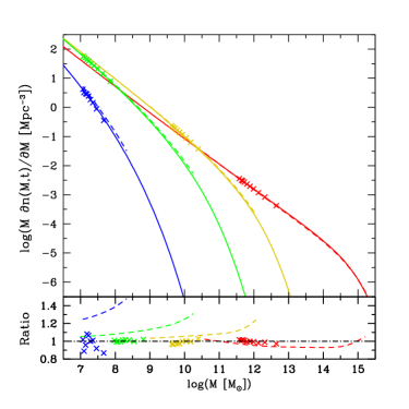
Figure 4: MFs predicted for haloes with FoF(0.2) masses (solid lines), compared to Warren et al. (2006) analytic fits to the MFs of simulated haloes (dashed lines) at $z=20$ (blue lines), 10 (green lines), 5 (yellow lines) and $0$ (red lines), from left to right. The dashed curves cover the ranges analysed in simulations. The ratios in the bottom panel are with respect to the theoretical predictions. Points are the raw data obtained by Lukić et al. (2007) in simulations with box sizes around $\sim 128(1+z)^{-1}$ Mpc$/h$ giving the best common resolution at all $z$’s.

But the density $N({R_{\rm f}},\delta_{\rm mi})$ includes all peaks, while $N^{\rm nn}({R_{\rm f}},\delta_{\rm mi})$ in equation (13) refers only to non-nested ones. Hence, we must correct $N({R_{\rm f}},\delta_{\rm mi})$ for nesting. This is achieved by solving the Volterra integral equation

$$N^{\rm nn}({R_{\rm f}},\delta_{\rm mi})=N({R_{\rm f}},\delta_{\rm mi})~{}~{}~{}~{}~{}~{}~{}~{}~{}~{}~{}~{}~{}~{}~{}~{}~{}~{}~{}~{}~{}~{}~{}~{}~{}~{}~{}~{}~{}~{}~{}~{}~{}~{}~{}~{}$$

$$-\frac{1}{\bar{\rho}_{\rm i}}\!\!\int_{R_{\rm f}}^{\infty}\!\!\!{\rm d}R\,N^{\rm nn}(R,\delta_{\rm mi})M(R,\delta_{\rm mi})N^{\rm nn}({R_{\rm f}},\delta_{\rm mi}|R,\delta_{\rm mi}),$$ (15)

where the second term on the right gives the number density of peaks with $\delta_{\rm mi}$ per infinitesimal scale around ${R_{\rm f}}$ nested into non-nested peaks with identical density contrast at any larger scale. The conditional number density of peaks with $\delta_{\rm mi}$ per infinitesimal scale around ${R_{\rm f}}$ subject to being located in the collapsing cloud of non-nested peaks with $\delta_{\rm mi}$ at $R>{R_{\rm f}}$, $N^{\rm nn}({R_{\rm f}},\delta_{\rm mi}|R,\delta_{\rm mi})$, is the integral over $r$ out to the radius, in units of $q{R_{\rm f}}$, of collapsing clouds of the conditional number density of peaks subject to identical conditions and the additional one of being located at a distance $r$ from a background peak with $\delta_{\rm mi}$ at $R$, $N({R_{\rm f}},\delta_{\rm mi}|R,\delta_{\rm mi},r)$,

$$N^{\rm nn}({R_{\rm f}},\delta_{\rm mi}|R,\delta)=\frac{3}{C}\int_{0}^{1}{\rm d}r\,r^{2}N({R_{\rm f}},\delta_{\rm mi}|R,\delta,r)\,.$$ (16)

In equation (16), the factor

$$C\equiv\frac{4\pi s^{3}N^{\rm nn}(R,\delta_{\rm mi})}{N({R_{\rm f}},\delta_{\rm mi})}\int_{0}^{s_{\rm int}}{\rm d}r\,r^{2}\,N({R_{\rm f}},\delta_{\rm mi}|R,\delta_{\rm mi},r)\,,$$ (17)

where $s_{\rm int}$ is the mean separation, in units of $q{R_{\rm f}}$, between non-nested peaks, is to correct for the overcounting of background peaks as those in $N({R_{\rm f}},\delta_{\rm mi}|R,\delta_{\rm mi},r)$ are not corrected for nesting. As in the case of the ordinary density of peaks $N({R_{\rm f}},\delta_{\rm mi})$, the conditional density $N({R_{\rm f}},\delta_{\rm mi}|R,\delta_{\rm mi},r)$ is the integral over all $x$ and over $\nu$ in the range given by the condition (14) of the conditional number density of peaks per infinitesimal values of $\nu$ and $x$ subject to being located at a distance $r$ from a background peak with $\nu^{\prime}$, ${\cal N}(\nu,x|\nu^{\prime},r)$, also provided by BBKS.

Using this prescription, every function $q(M,t_{0})$ obtained above for each value of $\delta_{\rm m}(t_{0})$ will give rise to one possible MF, although not necessarily satisfying the right normalisation condition

$$\bar{\rho}=\int_{0}^{\infty}M({R_{\rm f}})\;N^{\rm nn}({R_{\rm f}},\delta_{\rm mi})\;{\rm d}{R_{\rm f}}\,.$$ (18)

Thus, imposing this constraint, we can determine the right value of $\delta_{\rm m}(t_{0})$ and the corresponding function $q(M,t_{0})$. And repeating the same procedure at any time $t$, we can determine the whole functions $\delta_{\rm m}(t)$ and $q(M,t)$.

For FoF(0.2) or more exactly FoF(0.19) masses, the functions $\delta_{\rm m}(t)$ and $q(M,t)$ are found to be identical to those for SO($\Delta_{\rm vir}$) masses and take the form

$$\delta_{\rm m}(t)=\delta_{\rm c}(t)\frac{[a(t)]^{1.0628}}{D(t)}\,$$ (19)

$$q(M,t)\approx\left[Q(M)\frac{\sigma_{0}^{\rm TH}(M,t)}{\sigma_{0}(M,t)}\right]^{-2/[n(M)+3]}\,,$$ (20)

where $a(t)$ is the cosmic scale factor, $\delta_{\rm c}(t)$ is the density contrast for spherical collapse at $t$, $\sigma_{0}^{\rm TH}(M,t)$ is the top-hat 0th order linear spectral moment at $t$ related to $\sigma_{0}(M,t)$ through

$$\frac{\sigma^{\rm TH}_{0}(M,t)}{\sigma_{0}(M,t)}=1-0.0682\left[\frac{D(t)}{D(t_{0})}\right]^{2}\nu\,.$$ (21)

$n(M)$ is the effective spectral index at $M$ and $Q(M)$ is defined as

$$Q^{2}(M)=\frac{\int_{0}^{\infty}{\rm d}x\,x^{2+n(M)}\,W^{2}_{\rm G}(x)}{\int_{0}^{\infty}{\rm d}x\,x^{2+n(M)}\,W^{2}_{\rm TH}(x)}\,,$$ (22)

$W_{\rm TH}(x)$ and $W_{\rm G}(x)$ being the Fourier transforms of the top-hat and Gaussian windows of radius $x/k$, respectively. Expression (20) is approximate as it follows from the more fundamental relation (21), assuming the linear spectrum $P(k)$ equal to a power-law with spectral index equal to the effective one $n(M)$. This means that for the CDM spectrum both $n$ and $Q$ depend slightly on $M$. However, $q(M,t)$ is only needed to calculate $\sigma_{0}(M,t)$, which can be readily inferred from the well-known value of $\sigma_{0}^{\rm TH}(M,t)$ from the exact relation (21).

The MF for FoF(0.19) or SO($\Delta_{\rm vir}$) masses is compared in Figure 4 to the MFs of simulated FoF(0.2) haloes at three redshifts encompassing the interval studied by Lukić et al. (2007). Once again, there is overall agreement, particularly if we directly compare the theoretical predictions with the empirical data. Peaks with very low $\nu$’s will often be disrupted by the velocity shear caused by massive neighbours. But peaks suffering such strong tides will be nested, so they will not counted in the MF. This explains why the theoretical MF is well-behaved even at small masses.

4 Summary and Conclusions

Using simple consistency arguments, we have fixed the one-to-one correspondence between haloes and non-nested peaks for two popular halo mass definitions, allowing one to determine the mean spherically averaged density profile and MF of haloes by means of the CUSP formalism. The predictions found for SO($\Delta_{\rm vir}$) and FoF(0.2) masses in the concordance $\Lambda$CDM model are in good agreement with the results of numerical simulations.

The CUSP formalism is essentially exact and can be used to derive all typical halo properties such as the shape and kinematics (Salvador-Solé et al., 2012b). Moreover it is valid beyond the radius, mass and redshift ranges covered by simulations and can be applied to cold as well as warm dark matter cosmologies (Viñas et al., 2012). It thus has a wide variety of applications. Furthermore, it allows one to unambiguously show that accreting haloes grow inside-out and their structure is independent of their aggregation history (Juan et al., 2013).

ACKNOWLEDGEMENTS

This work was supported by the Spanish DGES AYA 2009-12792-C03-01 and AYA2012-39168-C03-02 and the Catalan DIUE 2009SGR00217. One of us, EJ, was beneficiary of the grant BES-2010-035483.

References

- Appel & Jones (1990) Appel L. & Jones B. J. T., 1990, MNRAS, 245, 522
- Ascasibar et al. (2004) Ascasibar Y., Yepes G., Gottlöber S., Müller V., 2004, MNRAS, 352, 1109
- Avila-Reese et al. (1998) Avila-Reese V., Firmani C., Hernández X., 1998, ApJ, 505, 37
- Bardeen et al. (1986) Bardeen J. M., Bond J. R., Kaiser N., Szalay A. S., 1986, ApJ, 304, 15 (BBKS)
- Bond (1988) Bond J. R. in Unrhu W. G., Semenov W. G., eds., The Early Universe, Reidel, Dordrecht, p. 283
- Bond et al. (1991) Bond J. R., Cole S., Efstathiou G., Kaiser N., 1991, ApJ, 379, 440
- Bond & Myers (1991) Bond, J. R. & Myers S. T., 1996, ApJS, 103, 41
- Colafrancesco et al. (1989) Colafrancesco S., Lucchin F., Matarrese S., 1989, ApJ, 345, 3
- Del Popolo et al. (2000) Del Popolo A., Gambera M., Recami E., Spedicato E., 2000, A&A, 353, 427
- Doroshkevich (1970) Doroshkevich A. G., 1970, Astrofizika, 6, 581
- Juan et al. (2013) Juan E., Salvador-Solé E., Manrique A., 2014, MNRAS submitted
- Frenk & White (2012) Frenk C. S. & White S. D. M., 2012, Annalen der Physik, 524, 507
- Gunn & Gott (1972) Gunn J. E. & Gott J. R., 1972, ApJ, 176, 1
- Hanami (2001) Hanami H., 2001, MNRAS, 327, 721
- Hahn & Paranjape (2013) Hahn O., Paranjape A., 2014, MNRAS, 438, 878
- Lacey & Cole (1994) Lacey C. & Cole S., 1994, MNRAS, 271, 676
- Ludlow & Porciani (2011) Ludlow A. D., & Porciani C., 2011, MNRAS, 413, 1961
- Lukić et al. (2007) Lukić Z., Heitmann K., Habib S., Bashinsky, S., Ricker P., ApJ, 671, 1160
- Maggiore & Riotto (2010) Maggiore M. & Riotto A., 2010, ApJ, 717, 515
- Manrique & Salvador-Solé (1995) Manrique A. & Salvador-Solé E., 1995, ApJ, 453, 6 (MSS)
- Manrique et al. (1998) Manrique A., Raig A., Solanes J. M., González-Casado G., Stein P., Salvador-Solé E., 1998, ApJ, 499, 548
- Navarro et al. (1997) Navarro J. F., Frenk C. S. & White S. D. M., 1997, ApJ, 490, 493
- Paranjape & Sheth (2012) Paranjape A. & Sheth R. K., 2012, MNRAS, 426, 2789
- Peacock & Heavens (1990) Peacock, J. A. & Heavens A. F., 1990, MNRAS, 243, 133
- Porciani et al. (2002) Porciani C., Dekel A., Hoffman Y. 2002, MNRAS, 332, 325
- Press & Schechter (1974) Press W. H. & Schechter P., 1974, ApJ, 187, 425
- Salvador-Solé et al. (2012a) Salvador-Solé E., Viñas J., Manrique A., Serra S., 2012a, MNRAS, 423, 2190 (SVMS)
- Salvador-Solé et al. (2012b) Salvador-Solé E., Serra S., Manrique A., González-Casado, G., 2012b, MNRAS, 424, 3129
- Sheth & Tormen (2002) Sheth R. K. & Tormen G., 2002, MNRAS, 329, 61
- Sugiyama (1995) Sugiyama, N. 1995, ApJS, 100, 281
- Viñas et al. (2012) Viñas J., Salvador-Solé E., Manrique, A., 2012, MNRAS, 424, L6
- Warren et al. (2006) Warren M. S., Abazajian K., Holz D. E., Teodoro L., 2006, ApJ, 646, 881
- Zhao et al. (2009) Zhao, D. H., Jing, Y. P., Mo, H. J., Börner, G. 2009, ApJ, 707, 354