Ionization compression impact on dense gas distribution and star formation

Abstract

Aims. The expansion of hot ionized gas from an H ii region into a molecular cloud compresses the material and leads to the formation of dense continuous layers as well as pillars and globules in the interaction zone. $Herschel$ imaging in the far-infrared (FIR) confirmed the presence of these dense features – potential sites of star-formation – at the edges of H ii regions. This feedback should also impact the probability distribution function (PDF) of the column density around the ionized gas. We aim to quantify this effect and discuss its potential link to the Core and Initial Mass Function (CMF/IMF).

Methods. We used in a systematic way $Herschel$ column density maps of several regions observed within the HOBYS key program: M16, the Rosette and Vela C molecular cloud, and the RCW 120 H ii region. We computed the PDFs in concentric disks around the main ionizing sources, determined their properties, and discuss the effect of ionization pressure on the distribution of the column density.

Results. We fitted the column density PDFs of all clouds with two lognormal distributions, since they present a ’double-peak’ or enlarged shape in the PDF. Our interpretation is that the lowest part of the column density distribution describes the turbulent molecular gas while the second peak corresponds to a compression zone induced by the expansion of the ionized gas into the turbulent molecular cloud. Such a double-peak is not visible for all clouds associated with ionization fronts but depends on the relative importance of ionization-pressure and turbulent ram pressure. A power-law tail is present for higher column densities, generally ascribed to the effect of gravity. The condensations at the edge of the ionized gas have a steep compressed radial profile, sometimes recognizable in the flattening of the power-law tail. This could lead to an unambiguous criterion able to disentangle triggered from pre-existing star formation.

Conclusions. In the context of the gravo-turbulent scenario for the origin of the CMF/IMF, the double peaked/enlarged shape of the PDF may impact the formation of objects at both the low-mass and the high-mass end of the CMF/IMF. In particular a broader PDF is required by the gravo-turbulent scenario to fit properly the IMF with a reasonable initial Mach number for the molecular cloud. Since other physical processes (e.g. the equation of state and the variations among the core properties) have already been suggested to broaden the PDF, the relative importance of the different effects remains an open question.

1 Introduction

Table 1: Molecular cloud parameters.

Cloud	Distance	Res.a	$\langle N(H_{2})\rangle^{b}$	Massc	$\langle T\rangle^{d}$	$\langle UV-flux\rangle^{e}$	r1, r2, r3, r4 f
	[kpc]	[pc]	[1022 cm-2]	[104 M⊙]	[K]	[G∘]	[pc]
M16	1.8	0.35	1.23	37.0	10.7 (6-23)	280 (20-1.8 104)	3, 5, 10, 15
Rosette	1.6	0.28	0.31	9.9	23.4 (12-36)	10 (1-104)	20, 25, 39, 54
RCW120	1.3	0.23	0.29	0.6	17.2 (13-25)	125 (4-8000)	2.5, 4.3, 5.5, 6.8
Vela C/RCW36	0.7	0.12	0.75	3.1	14.7 (11-29)	230 (50-1.5 104)	1.4, 3.2, 5.2, 6.6

^aSpatial resolution scale of the column density map (37^′′).
^bAveraged (over the whole map) column density of gas and dust, assuming a gas to dust ratio of 100. Note that these values may differ from the average value in the largest disks (regions 1+2+3+4) used for the PDFs.
^cTotal mass from column density map above N(H₂)=10²¹ cm^-2 using the conversion formula N(H₂)/$A_{V}$=0.94$\times$10²¹ cm^-2 mag^-1 (Bohlin et al., 1978).
^dAverage dust temperature (total range in parenthesis) from Herschel data.
^eAverage and min/max UV-flux (Schneider, priv.comm.) in Habing field, determined using the 70 $\mu$m and 160 $\mu$m Herschel flux. Details of the method are described in Roccatagliata et al. (2013). For RCW120, the typical value in the PDR-zone is 1-2 10³ G_∘, consistent with what determined by Rodón et al. (in prep.) using the spectral type of the exciting star.
^f Radii of the different disks used to compute the PDFs.

The role of density compression by the expansion of ionized gas into a molecular cloud has been discussed since the pioneering theoretical work of Elmegreen & Lada (1977). Dense features are observed at the edge of H ii regions, i.e., condensations (e.g. Deharveng et al., 2009; Zavagno et al., 2010), globules (e.g. Schneider et al., 2012b), and pillars (e.g. Hester et al., 1996; Schneider et al., 2010b). Although many models and numerical simulations have been able to explain how small structures can form (see Bertoldi, 1989; Lefloch & Lazareff, 1994; Miao et al., 2006, 2009; Mackey & Lim, 2010; Bisbas et al., 2011; Gritschneder et al., 2010; Haworth & Harries, 2011; Tremblin et al., 2012a, b), the question remains whether they are triggered or pre-existing. Simulation on the molecular cloud scale showed that the impact of high-mass stars on the molecular gas can enhance star formation (Dale et al., 2007) or that the impact is rather negligible (see Dale & Bonnell, 2011), depending on the physical properties of the cloud. In Tremblin et al. (2012b), we showed that the key parameter to understand the impact of a high-mass star on a molecular cloud is the ratio of the ionized-gas pressure to the ram pressure of the turbulence of the cloud. When the ionized-gas pressure dominates, compression from ionization is important, whereas the inverse leads to a compression dominated by the effect of turbulence. Turbulent compression has been intensively studied in the past few years thanks to simulations of isothermal supersonic turbulence (see Vázquez-Semadeni, 1994; Padoan et al., 1997; Kritsuk et al., 2007; Vázquez-Semadeni et al., 2008; Federrath et al., 2008, 2010). They showed that the probability distribution function of the density (density PDF) is well approximated by a lognormal form. Deviations from the lognormal shape – mostly in the form of power-law tails – were seen in simulations of compressible turbulence of a non-isothermal gas distribution (Passot & Vázquez-Semadeni, 1998), and/or in models including self-gravity (Klessen et al., 2000; Kritsuk et al., 2011; Federrath & Klessen, 2013). The effect of magnetic fields on the density PDF was found to be less important, generally reducing the standard deviation (Molina et al., 2012; Federrath & Klessen, 2012, 2013).

The impact of ionization on a turbulent velocity field was studied by Gritschneder et al. (2010) and the effect of ionization compression on the PDF in turbulent simulations has been investigated only recently by Tremblin et al. (2012b). They showed that when the ionized-gas pressure is larger than the ram pressure of the turbulence, a second peak in the PDF forms at high densities in addition to the lognormal shape. Observationally, this second peak caused by the compression from the ionized-gas pressure has been identified in the Rosette Nebula by Schneider et al. (2012a). But thanks to recent FIR-observations with the Herschel space telescope, it is now possible to study the column density PDF of the cold and warm molecular gas in high-mass star-forming regions, in which compression from ionization is likely to take place. Such regions are observed within the HOBYS key program (see Motte et al., 2010, 2012) and our study focuses on typical examples, i.e. the Rosette (Motte et al., 2010; Schneider et al., 2010b) and M16 molecular clouds (Hill et al., 2012b), and the H ii regions RCW 120 (Zavagno et al., 2010; Anderson et al., 2010, 2012) and RCW 36 (in the Vela C molecular cloud, Hill et al., 2011; Minier et al., 2013).

We determined the PDFs in areas of four concentric disks around the H ii regions present in these clouds in order to study the large-scale effect of the ionization on the cold molecular gas. The first disk always contains the OB cluster region and includes the closest dense structures of the molecular cloud. The centre of the disk is not the main ionizing source but corresponds to the approximate centre of the H$\alpha$ emission that is also approximately the centre of the spherical column density structures seen at the edge of the cavity in the Herschel maps. For Rosette and M16, the other disks are enlarged depending of the various dense structures present in the column density maps (37^′′ angular resolution), up to the largest disks that contain most of the maps. This choice allows us to study the evolution of the shape of the PDF in function of the column density structures that are included in the disks. For RCW 120 and RCW 36, less dense structures can be identified and the different radius are regularly spaced between the inner disk and the largest one reaching the edge of the observed map. Overall, the parameters of the fits of the PDFs have only little dependence on the precise choice of the radii of the disks (given in Table 1) as long as they include the same dense column density structures that can be seen in the Herschel maps (see an example for Rosette in Appendix A). We first present and validate the method on the M16 molecular cloud (Sect. 2), before showing the results on the Rosette Nebula (Sect. 3). Both of these regions are relatively large and their H ii region extended ($\approx$ 10-20 pc). However, their mass and the incident UV-flux is rather different (see Table 1). Finally, we study smaller-scale H ii regions, RCW 120 and RCW 36 (Sect. 4 and 5), that are only $\approx$1 pc large and have lower masses. This approach allows us to explore the compression effect over one order of magnitude each of spatial scale, mass, and incident UV-flux.

2 M16

M16 is located in the constellation of Serpens at 1.8 kpc from the Sun (Bonatto et al., 2006). The young stellar cluster NGC 6611 is ionizing the molecular gas of this star forming region. The principal ionizing sources are one O4 and one O5 stars whose combined ionizing flux is of order $2\times 10^{50}$ s^-1 (Hester et al., 1996; White et al., 1999). The discovery of pillars of gas in M16 by the Hubble space Telescope (Hester et al., 1996) popularized this region by naming it “Pillars of Creation”. Many spectral line studies have been performed on the cloud (see Pound, 1998; White et al., 1999; Allen et al., 1999; Urquhart et al., 2003, among others). The velocity of the CO line emission for the pillars is found between $\sim$20 and $\sim$30 km s^-1 (White et al., 1999). These authors suggest that emission around 29 km s^-1 is probably unrelated to the pillars. However with regard to the vicinity of the velocity to the cloud’s bulk emission and its spatial correlation (see their Fig. 8), a physical relation with the rest of the cloud is very likely. We thus do not expect the Herschel column density map to be strongly affected by line-of-sight (LOS) confusion. Recently, Flagey et al. (2011) measured dust spectral energy distributions (SEDs) thanks to Spitzer data. They show that the SED cannot be accounted for by interstellar dust heating by UV radiation but an additional source of radiation is needed to match the mid-IR flux. They proposed two explanations for this source of pressure: stellar winds or a supernova remnant. Herschel provides new observations on the region and Hill et al. (2012b) studied in detail the impact of the ionizing source on the temperature of the molecular gas. Heating is observed in regions with $n_{H_{2}}\approx 10^{5}-10^{6}$ cm^-3 thus impacting the initial conditions of the star-forming sites. We use the same Herschel map to study the PDF of the cold molecular gas at the interface with the H ii region. The column density map of the M16 molecular cloud (and of the other regions) was made by fitting pixel-by-pixel the spectral energy distribution (SED) of a greybody to the Herschel wavebands between 160 and 500 $\mu$m (at the same 37^′′ resolution), assuming the dust opacity law of Hildebrand (1983) and a spectral index $\beta$ of 2.

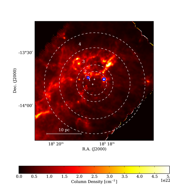
Figure 1: M16 Herschel column density map (Hill et al., 2012b). The circles indicate the different regions used for the PDFs. The white crosses indicate the position of the main ionizing sources. The limit of the H$\alpha$ emission is inside region 1+2+3 showing approximatively the limit of the H ii region (although the H ii region is not spherical in M16). The blue circles indicate the position of the dense condensations identified in the power-law tail of the PDF of region 1.

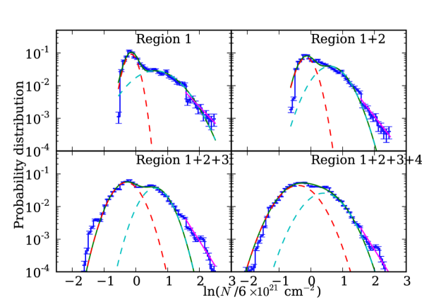
Figure 2: M16 PDFs on the four regions indicated in Fig. 1. The multi-component fit (green curve) is done using the sum of two lognormal distributions (red and blue dashed curves, see Eq. 1) and a power law at high column densities (magenta line, see Eq. 2). The error-bars are computed assuming Poisson noise in each bin of the distribution.

.
Region $\eta_{0}$ $p_{0}$ $\sigma_{0}$ $\eta_{1}$ $p_{1}$ $\sigma_{1}$ $m$ 1 -0.15 0.042 0.18 0.60 0.044 0.61 -2.33 1+2 -0.15 0.043 0.23 0.60 0.042 0.42 -2.88 1+2+3 -0.3 0.049 0.36 0.6 0.033 0.36 -3.54 1+2+3+4 -0.4 0.052 0.47 0.4 0.031 0.49 -3.55

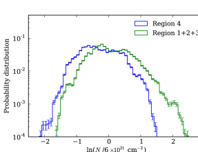
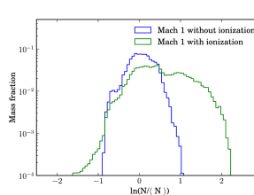
Table 2: Parameters of the fits of the PDFs in Fig. 3.

Figure 3: Left: M16 column density PDFs on region 1+2+3 and region 4 in Fig. 1. Right: Column density PDFs of the simulation of the ionization of a Mach-1 turbulent cloud (without self-gravity). The excess at high-density and the double-peaked distribution can be identified both in observations and numerical simulations.

Figure 1 shows the different subregions in M16 used for the PDFs plotted in Fig. 3. While the statistical Poisson error for the distribution is low (error bars are shown for the different PDFs) due to the large pixel statistics, there are systematic errors that influence the shape of the PDF. First, the assumption of isothermality along the line of sight for fitting the pixel-to-pixel SED to derive the column density is not fully justified. Clouds with feedback due to radiation clearly show temperature variations. For M16, a temperature gradient from $\sim$23 K to $\sim$16 K was found (Hill et al., 2012b). Second, the opacity increases towards higher column densities (Molina et al., 2012) which leads to a narrower PDF and a steeper slope of the power-law tail for high densities. It is important to exclude – or at least to quantify – possible line-of-sight (LOS) confusion that may result in a superposition of several PDFs from different clouds. This effect was already proposed by Lombardi et al. (2006) for the Pipe molecular cloud. It is necessary to use complementary spectroscopic data (preferentially atomic hydrogen or low-J CO) to well define the velocity range of the cloud emission. Examples of how to estimate the contribution of foreground and background clouds in Herschel column density maps are given in Rivera-Ingraham et al. (2013) and Russeil et al. (2013). In the case of M16, we do not expect the maps to be strongly affected by LOS confusion based on the CO line emission obtained by White et al. (1999).

Each disk contains the smaller ones, therefore, Fig. 3 shows the evolution of the shape of the PDF while increasing the radius of the disk around the ionizing sources. The first disk (region 1) contains the ionizing sources and the dense column density structures up to the massive young stellar object at the west of the ionizing sources (blue circle). The second disk (region 1+2) extends up to the base of the pillars of creation, the third disk (region 1+2+3) includes the whole dense structure at the north-west of the cavity (northern filament in Hill et al., 2012b), and the fourth disk (region 1+2+3+4) reaches the edge of the map. In all the regions a double peak is clearly identified, especially in region 1+2+3. In order to locate the position of the compressed gas, we plot the PDF of region 1+2+3 and the PDF of region 4 in Fig. 3. This region is an annulus that represents the outward parts of the cloud that should not be too much affected by the ionization. However a dense component is still present and corresponds to the eastern filament identified in Hill et al. (2012b). Apart from this filament, most of the compressed material in the second peak in the PDF in region 1+2+3 is not present in region 4, therefore the compression is likely to be linked with the ionized gas. To illustrate this point, we show in Fig. 3 the PDF obtained from the numerical simulation presented in Tremblin et al. (2012b). This simulation corresponds to the ionization of a turbulent cloud at Mach 1 (without self-gravity), in which the ionized-gas pressure is much greater than the turbulent ram pressure. The compression is therefore efficient and a second peak appears in the PDF of the column density of the gas. This simulation is not performed in the exact conditions of M16, that are not exactly known because of projection effects, however the double-peak is a global property both identified in these observations and numerical simulations.

Because of this compressed peak, the PDFs are fitted using two lognormal distributions:

$$p(\eta)=\frac{p_{0}}{\sqrt{2\pi\sigma_{0}^{2}}}\exp\left(\frac{-(\eta-\eta_{0})^{2}}{2\sigma_{0}^{2}}\right)+\frac{p_{1}}{\sqrt{2\pi\sigma_{1}^{2}}}\exp\left(\frac{-(\eta-\eta_{1})^{2}}{2\sigma_{1}^{2}}\right)$$ (1)

with $\eta=\ln(N_{H_{2}}/\langle N_{H_{2}}\rangle)$. $N_{H_{2}}$ is the column density and $\langle N_{H_{2}}\rangle$ is the average of the column density in the regions 1+2+3+4 $\langle N_{H_{2}}\rangle$=6$\times 10^{21}$ cm^-2 for M16 (note that this value is different from the averaged value on the whole map). We used $\eta$ with a natural logarithm to ease comparisons with previous works (e.g. Federrath & Klessen, 2013). $\eta_{i}$ and $\sigma_{i}$ are the peak value and standard deviation of each component, and $p_{i}$ is the integral of each component. The first lognormal component can be linked to the initial turbulent molecular cloud while the second lognormal component corresponds to a compression of the turbulent cloud whose source can be either ionization compression, colliding flows, or even winds, supernovas, etc. The high column-density part of the PDFs is fitted with a power law of power $m$ which corresponds to an equivalent spherical density profile of power $\alpha$ (see Federrath & Klessen, 2012; Schneider et al., 2013)

$$p(\eta) \propto N_{H_{2}}^{m}$$ (2)

$$\rho(r) \propto r^{-\alpha},\quad\mathrm{with}\quad\alpha=-2/m+1$$ (3)

Assuming spherical symmetry is a crude approximation for complex and large regions. However, if the pixels contributing to the power-law tail do belong to a single condensation this approximation is relatively accurate. Therefore we give the $m$ values in the tables of fitted parameters and only use the equivalent $\alpha$ values to discuss the results on single condensations or compare with previous works that used this conversion. A spherical self-gravitating cloud has an $\alpha$ value between 1.5-2 while higher values indicate a steeper profile influenced by compression. We point out that, for some PDFs, it could be argued that another choice of function (e.g. a lognormal and a two-step power law) could also give a good fit to the data, especially in region 1 in the case of M16. We will discuss in further detail in Sect. 6 the differences and motivations for a two-lognormal plus one power-law fit or a single lognormal plus a broken two-step power-law fit.

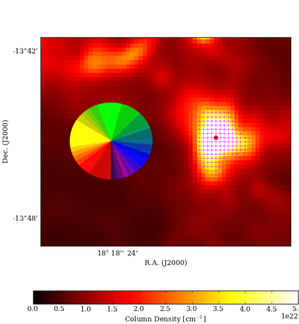
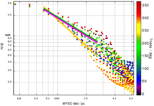
Figure 4: Top: zoom of the column density map on the western condensation. The magenta crosses indicate the pixels contributing to the power law of the PDF. The red dot is the position of the peak of the column density. The colormap is the color code used to show the orientation of the different profiles (e.g. green is north, yellow is east…). Bottom: Radial profiles of the column density of the western condensation. The color indicates the orientation of the profile. The power-law fits are performed around three different directions: north (180^∘) in green, east (270^∘) in yellow and south (360^∘) in purple. Each fit includes all the points in $\pm$ 40^∘ around the main direction.

Because of the number of parameters in Eq. 1, we fixed the peak values $\eta_{0}$ and $\eta_{1}$ based on the peak value of the low-density component seen in region 4 (Fig. 3) and the peak value of the compressed component seen in the concentric regions. After we have fixed these values $p_{i}$ and $\sigma_{i}$ are fitted to the observed distributions using a least-square method (Levenberg–Marquardt algorithm). We point out that the exact values of the fitted parameters may depend on the choice of $\eta_{0}$ and $\eta_{1}$, however the general behavior deduced in our analysis is robust to this choice. The different parameters deduced from the fits are given in Table 3. In M16, the lognormal fit of the low column density (red-dashed line in Fig. 3) cannot account for the high column densities, and the double peak is clearly visible even at high radius (e.g. region 1+2+3). The integral of the low-density peak $p_{0}$ increases with radius and the one of the compressed peak $p_{1}$ decreases with distance. This behavior suggests that the compression effect is more important close to the ionizing source and is indeed linked to the ionization. Furthermore, the decrease in the compressed-peak gas quantity is rather small even for region 1+2+3+4: the impact of the H ii region is a large-scale compression.

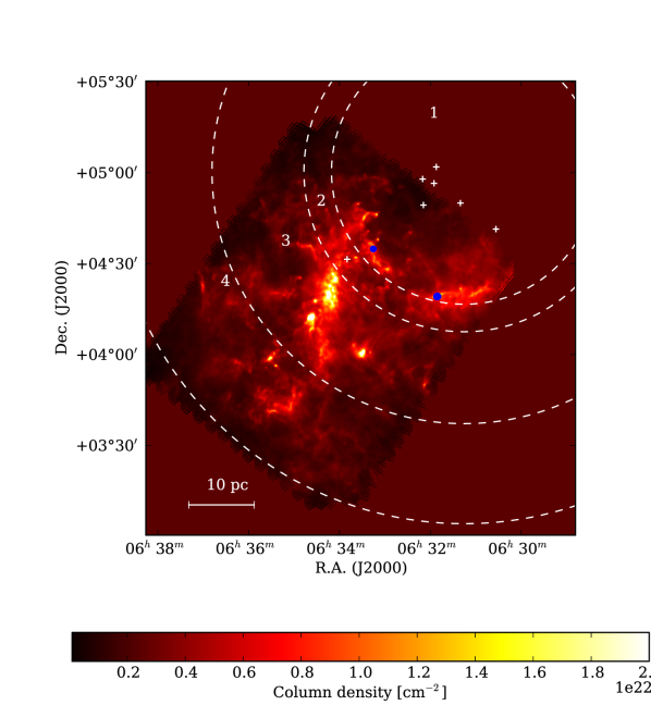
Figure 5: Rosette Herschel column density map (Schneider et al., 2012a). The circles indicate the different regions used for the PDFs. The white crosses indicate the position of the main ionizing sources, i.e. the most massive OB-stars from the NGC2244 cluster. The extension of the H$\alpha$ emission corresponds to region 1+2 but there is also a significant FUV radiation up to region 1+2+3 (see Schneider et al. in prep.). The blue circles indicates the position of the condensations identified in the PDF of region 1 and region 1+2.

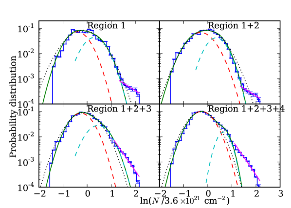
Figure 6: Rosette PDFs of the four regions indicated in Fig. 13. The multi-component fit is done using lognormal distributions (see Eq. 1) and a power law at high column densities (see Eq. 2). The black dotted line corresponds to a one-lognormal fit.

.
Region $\eta_{0}$ $p_{0}$ $\sigma_{0}$ $\eta_{1}$ $p_{1}$ $\sigma_{1}$ $\chi^{2}_{2L}$ 1 -0.41 0.07 0.39 0.30 0.04 0.38 250 1+2 -0.30 0.08 0.45 0.35 0.04 0.35 173 1+2+3 -0.26 0.09 0.39 0.45 0.03 0.40 236 1+2+3+4 -0.26 0.10 0.41 0.65 0.01 0.24 474 .
Region $\eta$ $p$ $\sigma$ $\chi^{2}_{1L}$ $m$ 1 -0.17 0.12 0.55 329 -1.36 1+2 -0.07 0.12 0.53 210 -1.36 1+2+3 -0.13 0.11 0.49 430 -3.19 1+2+3+4 -0.25 0.11 0.45 1411 -3.23

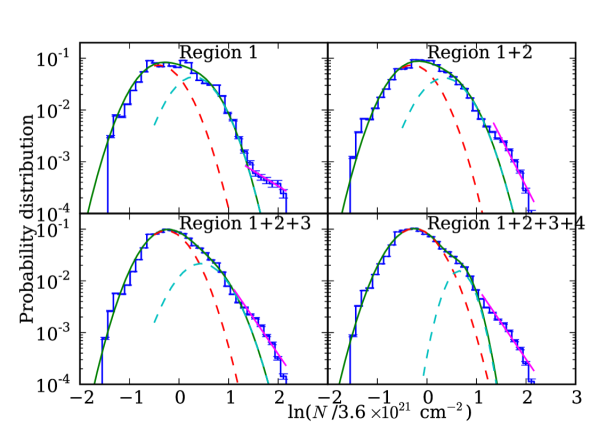
Figure 14: Rosette PDFs of the four regions indicated in Fig. 13. The multi-component fit is done using lognormal distributions (see Eq. 1) and a power law at high column densities (see Eq. 2).

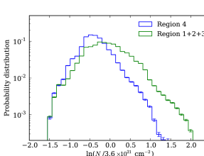
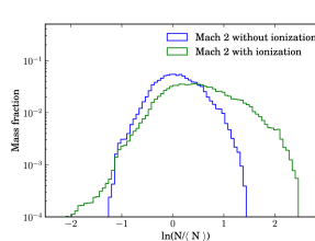
Table 3: Parameters of the two-lognormal fits of the PDFs in Fig. 14 and the corresponding reduced $\chi^{2}$ values.

Table 4: Parameters of the one-lognormal fits of the PDFs in Fig. 14 with the corresponding reduced $\chi^{2}$ values, and the exponents of the power-law fits at high column densities.

Figure 7: Left: Rosette column density PDFs on region 1+2+3 and region 4 in Fig. 13. Right: Column density PDFs of the simulation of the ionization of a Mach-2 turbulent cloud. The excess at high density is still visible however the two peaks merge to form an enlarged distribution. The simulations are without self-gravity, therefore there are no power-law tails in the simulated PDFs while they are present in the observations.

In principle, a second compressed lognormal peak can be linked to shock compression around an H ii region. This shock is likely to be driven by the expansion of the ionized gas. Gravitational instabilities – assuming that these are the most important physical processes for shaping the PDF – lead to a power-law tail and could not account for the compressed peak visible in region 1+2+3. The power-law tail can still be identified at higher column densities (starting approximately for $\ln(N_{H_{2}}/\langle N_{H_{2}}\rangle)>1.5$) where the distribution starts to deviate from the second log-normal. The slope fit leads to $\alpha$=1.86$\pm$0.05 in region 1 and decreases to $\alpha$=1.56$\pm$0.02 in region 1+2+3+4. These values are similar to those obtained in other regions like Aquila and Polaris (Schneider et al., 2013). In region 1, the pixels that contribute to the power law are part of two dense clumps indicated by blue circles in Fig. 1. Although the radial profiles of these clumps do show signs of compression, this effect is not reflected in the PDF, which mixes both condensations in the power-law tail. We give as an example in Fig. 4 the radial profiles of the massive western young stellar object (MYSO hereafter) as a function of the orientation. The profile is very steep on the side facing ionization (east side in yellow) with an $\alpha$ value of 2.3 (2.56 when the background column density is subtracted), while the profiles in the south and north directions (red and green) have an $\alpha$ value of 1.88 (1.99 when the background column density is subtracted) consistent with the influence of gravity. The average value is 2.25$\pm$0.02 suggesting that the compression on the MYSO is dominant. The same applies to the second condensation although the average $\alpha$ value is $\alpha$=1.76$\pm$0.02 suggesting that gravity is dominant. Thus, $\alpha$ values derived from the PDFs have to be taken with caution when different spherical structures are mixed in the same PDF. However when the PDF is computed on separated areas for the two condensations, the deduced $\alpha$ values are compatible with their averaged fitted profiles. The use of steeper profiles to identified compressed cores will be discussed in Sect. 6.

3 Rosette Nebula

The Rosette molecular cloud is located at 1.6 kpc from the Sun (Williams et al., 1994; Schneider et al., 1998a; Heyer et al., 2006) and is associated with a prominent H ii region, illuminated by the central cluster NGC 2244. The 17 OB stars of the cluster have a total Lyman-$\alpha$ luminosity of 3.8$\times$10⁵ L_⊙ (see Cox et al., 1990). The UV-flux is of the order of 100-200 G_∘ (Habing-field) (Schneider et al., 1998b) at the interface zone between H ii region and molecular cloud and decreases to a few G_∘ for the bulk emission deep ($\sim$30 pc) into the cloud. Photon dominated regions (PDRs) are found at the cloud surfaces where the UV-radiation shines directly onto the molecular cloud (see Schneider et al., 1998a, b). It is there where many pillars and globules are formed (see Schneider et al., 2010b, and Tremblin et al. in press). Although the total UV-field is low (on average only $\sim$10 G_∘, see Table 1) – compared to high-UV regions like Carina or Cygnus with up to 10⁵ G_∘ – the very clumpy and filamentary structure of the cloud enables a large penetration depth of UV-radiation so that PDRs are also found deep inside the cloud. The Rosette cloud contains several embedded infrared-clusters (see Poulton et al., 2008, and references therein), and is actively forming stars, indicated by a larger reservoir of clumps (Di Francesco et al., 2010), a large population of protostars (Hennemann et al., 2010), molecular outflows (White et al. in prep.), and a few candidate massive dense cores (Motte et al., 2010). There is a long ongoing-discussion whether star formation is triggered in Rosette, with a possible increasing age gradient from the ionization front into the cloud (see Schneider et al., 2010b, for a detailed discussion). For Rosette, the bulk emission of the cloud is at $\approx$16$\pm$6 km s^-1 (Williams et al., 1994; Schneider et al., 1998a) and there is no significant emission neither in HI nor CO outside this velocity range. Thus, the column density map is probably not very much affected by LOS confusion.

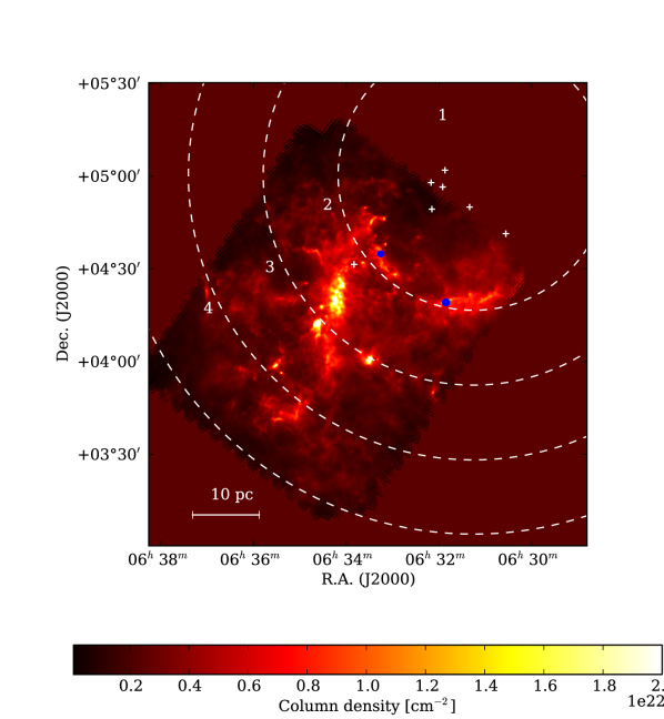
Figure 13: Rosette Herschel column density map (Schneider et al., 2012a). The circles indicate the different regions used for the PDFs. The white crosses indicate the position of the main ionizing sources, i.e. the most massive OB-stars from the NGC2244 cluster. The radius of the disks are regularly spaced between the inner and outer disks.

Schneider et al. (2012a) has already shown that a double peak in the PDF was found for the gas close to the border of the shell ($\approx$ 20 pc of radius). However, their distinctions into subregions were mainly based on morphology, so that here, we study the evolution of the PDF as a function of radius around the H ii region in a more systematic way, by taking the distribution in concentric disks around the bubble. In Fig. 13, we show the four different regions that are considered for the PDFs presented in Fig. 14. The first disk (region 1) contains the ionizing sources and the dense column density structures up to the massive young stellar object at the south of the ionizing sources (blue circle). The second disk (region 1+2) extends up to the northern part of the main star-forming region of Rosette (see Schneider et al., 2012a), the third disk (region 1+2+3) includes this star-forming region, and the fourth disk (region 1+2+3+4) reaches the edge of the map. In Fig. 7, we show the PDF of the region 1+2+3 and the annular region 4 in order to compare the compressed part that is influenced by an effect localized near the ionizing sources. The PDF of region 1+2+3 is not double-peaked as was seen for M16 and even the one of region 1 alone shows only a slight indication of a double-peak, less clearly than was presented in Schneider et al. (2012a). Indeed, in Schneider et al. (2012a), the selection of regions focused explicitly on the interaction zone (only a small part of our region 1) and thus revealed the double-peak. Taking a larger area adds more pixels that are not directly impacted by the ionization front (towards the south-west in our region 1) and thus dilutes the double-peak. For comparison we show also in Fig. 7 the PDFs of a simulated Mach-2 turbulent cloud exposed to ionization (Tremblin et al., 2012b). The PDF presents a similar shape where the two peaks merge to form an enlarged distribution. One could argue that these enlarged distributions can be fitted properly by a single lognormal component. We show in Fig. 14 such a fit (black-dotted line) and the corresponding parameters are given in Table 7 while the parameters of the two-lognormal fit are given in Table 7. The reduced $\chi^{2}$ values for both fits are computed assuming a Poisson noise in each bin. The corresponding error-bars are plotted in Fig. 14 but the pixel statistic is so large that the error-bars are small and barely visible in log-space. Such small error-bars explain the large values of the $\chi^{2}$ for both fits. This means that these regions have complex structures and physics that are not well represented by the fitting models. We performed a F-test to check that the two-lognormal fit provides a significant improvement (see Bevington & Robinson, 2003). The F values for the different regions are respectively 3.3, 2.6, 6.8, and 15 and the critical value is 3 for a false-rejection probability of 5 %. Therefore, the two-lognormal model gives a significantly better fit to the data especially in regions 1+2+3 and 1+2+3+4. In all regions, there is an excess of compressed gas compared to the PDF in the annular region 4. The integral of the compressed component $p_{1}$ in Table 7 decreases from 0.04 to 0.01 when the radius of the region increases. This behavior is expected: when the radius of the region increases, more and more unperturbed gas is added in the distribution while the compressed gas remains the same. Therefore the relative importance of the compressed gas decreases.

When this excess is taken into account by a second lognormal component in the fits in Fig. 14, a power-law deviation from the two-lognormal distribution is still visible and indicates the possible influence of gravity but at higher column densities. It is especially clear in regions 1 and 1+2 that the power-law deviation is occurring around $\eta$ $\approx$ 1.5, indicating the regime in which gravity starts to dominate. Assuming an equivalent spherical density distribution ($\rho\propto r^{-\alpha}$), a transition from an exponent $\alpha$ of 2.38$\pm$0.10 in regions 1 and 1+2 to a value of 1.62$\pm$0.08 in region 1+2+3+4 is derived from the power-law fits. This transition indicates that the ionization can have an influence even on the gravity-dominated regions that are in the PDR. Assuming spherical symmetry on large scale (regions 1+2+3 and 1+2+3+4) is a very crude approximation in these complex regions and a detailed analysis taking into account the Mach numbers is needed to study the interplay between other different processes. In region 1 and 1+2, the pixels that have a column density with $\eta$ higher than 1.5 correspond to two nearly spherical dense condensations in the Monoceros Ridge and in south dense region at the edge of the cavity (blue circles in Fig. 13) which were already identified as regions of gas compression at the cloud-nebula interface (Román-Zúñiga & Lada, 2008). As in M16, these $\alpha$ values have to be taken with caution since they mix different structures. Nevertheless, the high alpha value observed in regions close to the ionizing sources was already seen in other regions like the central, dense, high-mass star-forming ridge in the cloud NGC 6334 (Russeil et al., 2013) and more recently in Palau et al. (2013) (for the massive dense cores DR21-OH, AFGL 5142 and CB3). The transition from high values to low values typical of other clouds seems to indicate that the compression from ionization is also playing a role at high column densities where structures are expected to be gravitationally collapsing.

4 RCW 120

RCW 120 (Fig. 8) is an H ii region (see Rodgers et al., 1960; Zavagno et al., 2007) located at a distance of 1.3 kpc from the Sun and well studied by Spitzer (Deharveng et al., 2009) and Herschel (Zavagno et al., 2010; Anderson et al., 2010). Its circular shape led to the name of “the perfect bubble” (Deharveng et al., 2009), although the ionizing source, an O8 star (Martins et al., 2010), is not at the centre of the ionized sphere. Since the ionizing source is very close to the southern part of the bubble, it is probable that the expansion is asymmetric. The molecular gas is denser at the south than the north of the bubble, as indicated by the column density (see Fig. 8). Because of the asymmetry, the 1D model of collect and collapse is difficult to apply in the form presented in Elmegreen & Lada (1977). Among other regions, the dust properties of RCW 120 has been recently analyzed by Anderson et al. (2012) using Herschel observations. These authors found that the mass of the material in the PDR is compatible with the expected mass swept up during the expansion of the H ii region and that the FIR emission suggests that the bubble is a three-dimensional structure. We used in the present analysis the column density map derived by Anderson et al. (2012). We point out that the column density map of RCW120 is done by a fit in linear space rather than log space (as done for the other Herschel maps). However we do not expect this inconsistency to influence our results.

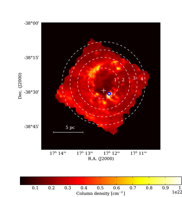
Figure 8: RCW 120 Herschel column density map (Anderson et al., 2012). The circles indicate the different regions used for the PDFs. The white cross indicates the position of the main ionizing source (O8 star). The extension of the H$\alpha$ emission and the limit of the H ii region is inside region 1. The blue circle indicates the position of the possible compressed core collapse identified in the PDFs.

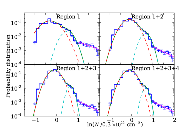
Figure 9: RCW 120 PDFs on the four regions indicated in Fig. 8. The multi-component fit is done using lognormal distributions (see Eq. 1) and a power law at high column densities (see Eq. 2).

.
Region $\eta_{0}$ $p_{0}$ $\sigma_{0}$ $\eta_{1}$ $p_{1}$ $\sigma_{1}$ $m$ 1 -0.3 0.12 0.36 0.5 0.014 0.24 -1.28 1+2 -0.1 0.12 0.29 0.65 0.008 0.19 -1.73 1+2+3 -0.1 0.13 0.25 0.65 0.005 0.14 -1.73 1+2+3+4 -0.1 0.13 0.13 0.65 0.003 0.13 -1.73

Table 5: Parameters of the fits of the PDFs in Fig. 5.

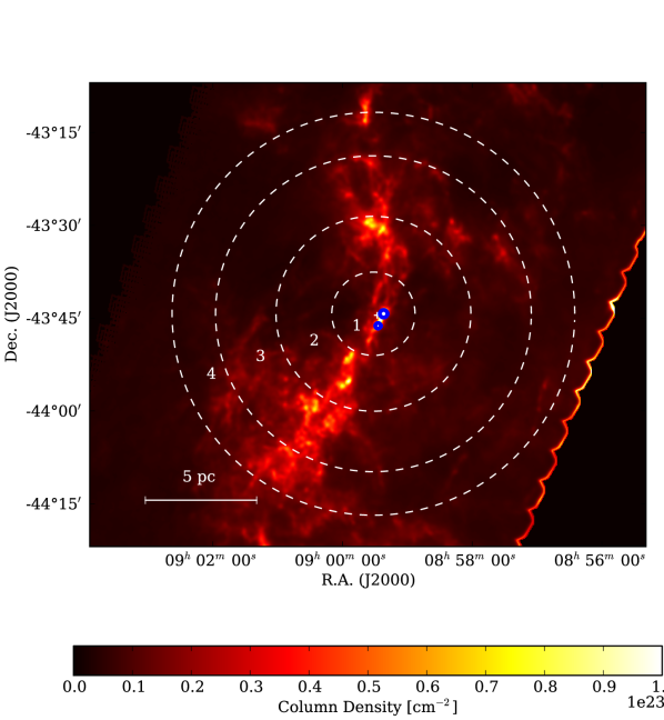
Figure 10: RCW 36 Herschel column density map (Minier et al., 2013). The circles indicate the different regions used for the PDFs. The white cross indicates the position of the main ionizing source. The limit of the H$\alpha$ emission and the limit of the H ii region are inside region 1. The blue circles indicate the positions of the condensations identified in the PDF of region 1.

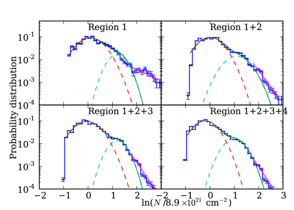
Figure 11: RCW 36 PDFs on the four regions indicated in Fig. 10. The multi-component fit is done using lognormal distributions (see Eq. 1) and a power law at high column densities (see Eq. 2).

.
Region $\eta_{0}$ $p_{0}$ $\sigma_{0}$ $\eta_{1}$ $p_{1}$ $\sigma_{1}$ $m$ 1 0.1 0.11 0.47 1.2 0.014 0.33 -1.12 1+2 0. 0.11 0.45 1.1 0.016 0.45 -3.28 1+2+3 -0.05 0.11 0.31 1.2 0.011 0.33 -3.65 1+2+3+4 -0.2 0.11 0.42 1.0 0.016 0.38 -3.70

Table 6: Parameters of the fits of the PDFs in Fig. 6.

In Fig. 8, we show the four different regions that are considered for the PDFs presented in Fig. 5. The parameters of the fits are listed in Table 5. The PDFs are well fitted by a two-component lognormal and the excess in the compressed component is clearly visible in regions 1+2+3 and 1+2+3+4. At high column densities, it is possible to identify the dense clump formed at the south west of the ionizing source in the dense part of the PDF (blue circle in Fig. 8). This clump is not part of the compressed component and the PDF is well fitted by a power-law suggesting the role of gravity. In region 1, the power-law fit leads to an exponent $\alpha$ of 2.56$\pm$0.17 that may indicate the role of ionization compression in the formation of this condensation and its collapse to form stars. The radial profile of the condensation has an exponent $\alpha$ of 2.39$\pm$0.01, which is in a good agreement with the value deduced from the PDF. If the gravitational collapse would have happened before, we would expect the exponent to be close to 2 and to be only marginally affected by the ionization since the ionizing front did not overwhelm the condensation. Indeed the numerical study in Minier et al. (2013) in the case of RCW 36 showed that the collapse of a condensation that is located in the shell is likely to be triggered. If the condensation had gravitationally collapsed prior to the passage of the ionization front, the condensation will be already sufficiently dense to resist the ionization front expansion. It would for example trigger the formation of a pillar rather than a condensation remaining in the shell. Furthermore a statistical argument based on the study of Thompson et al. (2012) also suggests that the dense condensation is linked to the H ii region. Based on the numerical study of Minier et al. (2013), the triggering can be confirmed by comparing the velocities of the condensation and the nearby shell. If the velocities are the same, the formation of the condensation is dynamically linked to the shell and likely to be triggered.

The amplitude of the compressed lognormal decreases when the radius of the region increases (see Table 6). This is consistent with the picture we got from Rosette and M16: the larger the region, the less important becomes the peak, because more and more unperturbed gas is added to the distribution. However, the decrease of the amplitude of the compressed peak is more important in the case of RCW 120 (from 0.014 to 0.003). This can be explained by the H ii region occupying a smaller part of the image than the large ionized bubbles in the Eagle and Rosette Nebula. The compression factor of the column density is typically of the order of 2 (given by $\exp(\eta_{1}-\eta_{0})$). That is rather low compared to the factor 20-30 expected from the 1D simulations of Zavagno et al. (2007). However the difference could be the result of a projection effect. Considering the size of the bubble which has a radius of 1.8 pc, we can assume that the thickness along the line of sight of the compressed layer is of the order of 1 pc. The cloud is at a column density of 10²³ cm^-2 and corresponds to a density of 3$\times$10³ cm^-3 integrated over a line of sight of 10 pc. The compressed layer has a column density of around $2\times 10^{23}$ cm^-2 which corresponds to a density of 6$\times$10⁴ cm^-3 integrated over 1 pc. Therefore we can get a compression of $\approx$ 20 if the line-of-sight thickness of the shell is ten times smaller than the thickness of the cloud. Therefore a factor of compression of 20-30 in density can result in a factor of compression of 2 in column density.

5 Vela C/RCW 36

RCW 36, at a distance of 700 pc from the Sun (Murphy & May, 1991), has the shape of an hourglass. At the centre, an embedded cluster, 2-3 Myr old, has 350 members with the most massive star being a type O8 or O9 (Baba et al., 2004). The cluster extends over a radius of 0.5 pc, with a stellar surface number density of 3000 stars pc^-2 within the central 0.1 pc. FIR emission and radio continuum emission are reported to be consistent with the presence of an H ii region (Verma et al., 1994). The star cluster has probably inflated the G265.151+1.454 H ii region (Caswell & Haynes, 1987) that is responsible for the H$\alpha$ emission originally observed by Rodgers et al. (1960). Looking at larger scales, RCW 36 is located within the Vela C molecular cloud that consists of an apparent network of column density filaments (Hill et al., 2011). Such filaments are star formation sites. Herschel observations of low-mass star-forming molecular clouds (e.g. Arzoumanian et al., 2011) show that stars form in supercritical filaments while Schneider et al. (2012a) propose that star-cluster formation sites correlate with filament network junctions. Among the networks of filaments in Vela C, there is a more prominent and elongated interstellar dust structure of $\approx$ 10 pc in length that is named the Centre-Ridge by Hill et al. (2011). It encompasses RCW 36, which is at its Southern end, a bipolar nebula surrounded by a dense ring of gas in the plane of the Centre-Ridge (Minier et al., 2013).

Figure 10 shows the Herschel column density map of RCW36 inside the Vela C molecular cloud with the different regions for which we determined the PDFs (Fig. 6 and Table 6). The first region corresponds to the extension of the ionized gas. The PDF presents two components, however, contrary to the other regions, the amplitude of the compressed peak does not decrease with increasing radius. In region 1, the high-density component consists of the dense ring close to the cluster (Minier et al., 2013), and the low-density one corresponds to the low-density medium that is present on each side of the bipolar nebula. The deviation at high densities ($\ln(N_{H_{2}}/\langle N_{H_{2}}\rangle)\approx 2$) corresponds to the dense condensations that are present in the ring and were also discussed in Minier et al. (2013). A power-law tail (although complex) for this range can be identified. Though the pixel statistic is small and the error larger, we tentatively determine a value of $\alpha$=2.80$\pm$0.23 which is much higher than 2. This high value is also consistent with the filamentary profile measured by Hill et al. (2012a) ($\alpha$=2.70$\pm$0.2). We checked the radial profiles of the densest and largest condensation and got an averaged fitted value of $\alpha$=2.30$\pm$0.11 (in some direction the profile has an alpha value of 2.83). We may have here the same situation as in RCW120 where the PDF also shows a clear excess for the highest densities due to individual compressed core collapse. This supports the previous study in Minier et al. (2013) showing that, based on the morphology of the regions, the gravitational collapse of these condensations (blue circles in Fig. 10) was likely to be triggered (also confirmed by the recent age determination of the different stellar populations done by Ellerbroek et al. (2013)). Furthermore, the exponent $\alpha$ decreases to a value of 1.54$\pm$0.02 in region 1+2+3+4. The region is so large that the dense small clumps contribute to the probability distribution at less than 10^-4 and therefore are not visible in the PDFs anymore. The dense compressed power-law tail is therefore only present in region 1 and probably linked to the ionization. In previous large-scale studies, e.g. the Vela C cloud (Hill et al. 2011), Rosette (Schneider et al. 2012), and NGC6334 (Russeil et al. 2013), it was not possible to distinguish whether the power-law tail arises from collapse of many cores and/or global collapse of clumps or filaments/ridges since both processes play a role. In smaller regions, we are less perturbed by a large amount of bulk gas that constitutes the PDF and global collapse may play a minor role. However, we emphasize that this finding remains slightly speculative and needs further detailed studies.

In any case, when the radius of the area increases, the low-density component remains the same and the amplitude of the high-density peak increases. This behavior is expected because the influence of the H ii region is limited to region 1 and in the other regions, the high-density component does not consist of the compressed ring anymore, but is dominated by the south-north elongated molecular cloud. When the radius is high, the area of the compressed ring around the H ii region is very small compared to the rest of the molecular cloud.

6 Discussion and interpretation

6.1 From large-scale to small-scale ionization compression

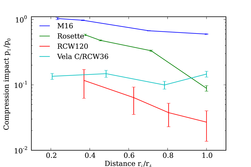
Figure 12: Radial evolution of the ratio of the number of pixels in the compressed peak to the number of pixel in the low-density peak $p_{1}/p_{0}$ for the four different clouds.

Based on the two-lognormal fits performed in the different regions, we define a compression parameter as the ratio of the number of pixels in the compressed component to the number of pixels in the low-density component. Figure 12 shows the evolution of this parameter as a function of radius for the four different clouds. For Rosette, M16, and for RCW 120, the compression impact decreases with increasing radius. Therefore, the compressed material is localized close to the ionizing sources and its relative volume decreases when the volume of the studied region increases.

At a first glance, it could be argued that dense gas is present close to ionizing sources because they were born in a dense environment formed e.g. by gravitational collapse or colliding flows. This first possibility is ruled out by the comparison made in M16 and Rosette between the dense column density excess in region 1+2+3 compared to region 4 (Fig. 3 and Fig. 7). This excess does not follow a power law as would be expected from gravitational collapse. In the second case, it is much more difficult to distinguish dense gas formed from colliding flows prior to the formation of the ionization sources and ionization compression that will happen after. However the Vela C molecular cloud offers the possibility to show how the difference can be inferred. For Vela C, the dense gas does not seem to be related to the ionizing sources as shown by Fig. 12. The ratio of dense gas to low-density gas is relatively constant at 15 % in the whole region. From the column density map, we derive an average density in the Vela C molecular ridge – assuming a thickness of the ridge of 1 pc – of $10^{4}$ cm^-3 while in the more extended low-density medium ($\sim$5 pc thickness) the density is $10^{2}$ cm^-3. The lognormal shape of the high-density component seen in regions 1+2+3 and 1+2+3+4 suggests that the ridge is formed by shock compression rather than gravitational instabilities. The ridge formation from shock compression caused by colliding flows was proposed in Vela (Hill et al., 2011) and also for example in IRDC G035.39-00.33 (Nguyen Luong et al., 2011) or W43 (Nguyen Luong et al., 2013). In this case, the ridge could be the result of converging flows at a density of around $10^{2}$ cm^-3 that collided at a Mach number $\sim$10 to compress the gas by two orders of magnitude, assuming isothermal gas. This estimation of the Mach number is rather close to the Mach number expected for the cold interstellar medium ($T_{c}$ $\approx$ 50-100 K for the cold neutral medium CNM) formed by the thermal instability inside the warm phase of the interstellar medium ($T_{w}$ $\approx$ 8000 K for the warm neutral medium WNM). Since the CNM has a typical velocity that is transonic relative to the sound speed in the WNM (see Audit & Hennebelle, 2010), the Mach number of the CNM is given by $M\approx\sqrt{T_{w}/T_{c}}\approx 10$. Therefore it is possible that the Vela C molecular ridge was formed by colliding flows whereas the dense gas in the three other regions M16, Rosette and RCW 120 is formed by ionization compression since its volume is inversely correlated with the distance from the ionizing sources.

On smaller scales, we have seen that in the inner regions with smaller pixel statistics, we can identify power-law tails that correspond to one or two dense condensations that have probably gravitationally collapsed. The PDF around these condensations and their radial profiles indicate $\alpha$ exponents higher than the free-fall value of 2. Therefore they could be examples of compressed core collapse triggered by the ionization compression. Although more studies are needed to confirm these results, this behavior could be the first unambiguous criterion that can make the difference between non-triggered (free-fall) and triggered (forced-fall) core collapse around H ii regions. It could also be generalized to any type of external compression (winds, supernovas…) whose source is identified.

6.2 The shape of double-peaked and broadened PDFs

The regions studied here – the Rosette and Eagle molecular clouds, and the RCW 36 and RCW 120 H ii regions – differ significantly in terms of mass (from $\sim$6$\times$10³ M_⊙ for RCW 120 to $\sim$4$\times$10⁵ M_⊙ for M16), temperature and incident UV-flux (with a low G_∘ cloud like Rosette in contrast to a bright cloud with a high G_∘ like M16), and size (a few pc for the small H ii regions up to $\sim$20 pc for the Rosette nebula). Nevertheless, they all show the same characteristic double-peaked and/or broadened PDFs. We argued that it is compression caused by the expansion of the ionized gas that causes a double peak in the column density PDF (in the case of the M16 molecular cloud) or an enlarged distribution when the second peak is close to the first one (in the case of the Rosette molecular cloud and RCW 120). As explained in the previous section, the Vela C molecular cloud presents a dense component probably formed by colliding flows that also broaden the PDF. The difference between this scenario and that of ionization compression can be inferred from the evolution of the compression parameter with increasing radius (see Fig. 12).

For Rosette, M16, and RCW 120, the compression parameter decreases when the radius of the region on which the PDF is computed increases. This is consistent with a compressed region localized at the edge of the ionized gas. When the radius increases, more and more unperturbed gas is added to the distribution. For more extended regions (Rosette and M16), the H ii regions are relatively large compared to the molecular cloud, and the effect and the compression is important even on the large scale (a few tens of parsecs) of the cloud. In contrast, RCW 120 is relatively small and the compression parameter is quite small compared to the other regions (see Fig. 12).

For these three ionization-compressed regions, we fitted the two-peaked and enlarged distributions with two lognormals. A simple approach can qualitatively justify the choice of a lognormal shape for the ionization-compressed component. The first component is enlarged by the turbulence of the cloud and its lognormal shape can be qualitatively understood (see Vázquez-Semadeni, 1994; Kevlahan & Pudritz, 2009). If a region of density $\rho_{0}$ is compressed by a shock of Mach number $M_{1}$, the new density is then $\rho_{1}=\rho_{0}M_{1}^{2}$. When a second shock compresses the region, the new density is $\rho_{2}=\rho_{1}M_{2}^{2}=\rho_{0}M_{1}^{2}M_{2}^{2}$ and so on… This process is additive with respect to $\ln(\rho)$ and if it is repetitive and random, we can expect that the logarithm of the density is a Gaussian thanks to the central limit theorem (hence, the density should be lognormal, see also Federrath et al. (2010)). There are some limits to this analysis (e.g. multiple compressive forces, see Hennebelle & Falgarone, 2012) but it is a straightforward way to understand the shape of the density distribution.

The same idea can be used to understand the shape of the double peak distribution for the surroundings of an H ii region. As explained in Tremblin et al. (2012b), there are two situations to consider, either the ionized-gas pressure is much greater than the ram pressure of turbulence, or turbulence dominates. In both cases, the Mach number of the shock driven by the H ii region is well approximated by

$$M_{\mathrm{io}}=\sqrt{\zeta}\frac{c_{II}}{c_{0}}\left(\frac{R_{s}}{r_{\mathrm{shell}}}\right)^{3/4}$$ (4)

where $c_{II}$ and $c_{0}$ are the sound speed in the ionized and shocked region respectively, $R_{s}$ is the initial Strömgren radius (computed for the initial averaged density around the ionizing source), $r_{\mathrm{shell}}$ the radius of the H ii region at the time considered, and $\zeta$ a parameter that is equal to two for a D-critical front (Kahn, 1954) and one for a weakly D-type front (see Minier et al., 2013, for the detailed calculation). At the beginning of the development of the H ii region, the ionizing front is D-critical and $r_{\mathrm{shell}}=R_{s}$. Therefore the Mach number is of the order of 40. Such level of turbulence is not observed in molecular clouds, hence there is always a period of time for which $M_{\mathrm{io}}\gg M_{i}$ where $M_{i}$ are the Mach numbers of the turbulent shocks in the molecular cloud. When the shock driven by the ionized gas passes, the gas is compressed and the log-density increases by $\ln(M_{\mathrm{io}}^{2})$. In an initial turbulent medium, the same analysis as Kevlahan & Pudritz (2009) can be applied to $\ln(\rho_{0})=\ln(\rho_{c})-\ln(M_{\mathrm{io}}^{2})$. Thanks to the central limit theorem, $\ln(\rho_{0})$ is a Gaussian and $\ln(\rho_{c})$ is a Gaussian shifted by a compression factor $\ln(M_{\mathrm{io}}^{2})$. Therefore, if sufficient material is accumulated in the shell, two lognormal peaks appear in the PDF. When the turbulence is high compared to the ionized-gas pressure, $M_{io}\approx M_{i}$ and the term added to the log-density appears as one shock among others in the turbulent medium. Therefore with the central limit theorem, the distribution of the log-density will be unchanged by the ionization-driven shock. This is exactly what was observed in the simulation of Tremblin et al. (2012b), the lognormal double-peaked PDF appears when the ionized-gas pressure is high relative to the turbulent ram pressure and at high turbulent level, the PDF is rather unchanged by the ionization. This explains also why in some clouds, no second peak is observed but only broadening by compression. A recent study of the Orion B molecular cloud (Schneider et al., 2013) showed that the PDF has a lognormal shape with a power-law tail but is a factor 1.5 broader than the one of a similar region (Aquila) that has the same Mach-number. The difference is that Orion B is exposed to a large-scale compression from a nearby OB-cluster (also seen in asymmetric column density profiles) while Aquila contains only a small internal H ii region. Another example is the Auriga-California cloud (Harvey et al., 2013) that shows a double-peak in the PDF. But this cloud is a low-mass star-forming region with only a B-star as ionizing source, so the total impact of the ionization front is smaller than for a cloud that is impacted by a whole OB-cluster. However – as outlined above – it is not the total energy contained in the shock expansion that decides whether a compressed layer is formed and visible in the PDF, but the interplay between ionized-gas pressure and turbulent ram pressure. We thus do not expect a double-peaked PDF for all clouds associated with OB-clusters.

On the other hand, a second break in the PDF power law can be observed in some clouds and linked to the feedback (e.g. W3, Rivera-Ingraham et al. submitted). These two breaks could mean that the PDFs can be fitted by a lognormal for the turbulent cloud, a first power law for the feedback compression and a second power law for the influence of gravity. As mentioned in Sect. 2, the inner region in M16 could also be well fitted by such a model. Although our approach here is slightly different we think that both methods are complementary. In the inner region, the scales are smaller and the compressed shell should be rather homogeneous. In this case, the statistic may not be sufficient to get a proper sampling of the turbulent compressed peak that is seen in the turbulent-ionized simulations. Therefore the column-density PDF of an homogeneous compressed shell could lead to a flat power-law for the compressed component in column density, and the gravity to a power law with a steeper slope, hence a two-step power law. On a larger scale, a sufficiently large range of turbulent motions will be taken into account and a better statistic will lead to a compressed lognormal component as seen in the turbulent-ionized simulations. Thus, depending on the scale or turbulent state of the region, the compressed component may be well approximated by a power law or a lognormal. In both cases, the compression by ionization does have an impact and leads to a broadened PDF.

6.3 Possible consequences of external compression for the IMF

Recently, Hennebelle & Chabrier (2008, 2009, 2013) proposed an analytical theory to derive the CMF/IMF (Core/Initial Mass Function) from the PDF of a gravo-turbulent molecular cloud. The central idea is that the shape of the IMF can be computed from any kind of PDF assuming that the global properties of the cloud are the determinant factor to set the final IMF. Therefore the typical shape of the Chabrier IMF (log-normal at low mass and a Salpeter power-law at high mass, see Chabrier, 2003) could be determined from the global properties of the gravo-turbulent cloud by computing the gas volumes sufficiently dense to collapse gravitationally. One direct implication of the present work is that the ionization compression affects the PDF around the ionized gas and consequently could also affect the CMF/IMF.

H ii regions are present in a vast number of molecular clouds, even in low-mass star-forming regions (e.g. the Cocoon Nebula in IC 5146, Arzoumanian et al. (2011) and W40 in Aquila, Bontemps et al. (2010); Könyves et al. (2010)). This type of feedback of high-mass stars is also thought to be one of the most important processes to disperse molecular clouds in our Galaxy (see Whitworth, 1979; Matzner, 2002). Considering the typical lifetime of molecular clouds ($\approx$ 10 Myr) and the typical time of the development of H ii regions ($\approx$ 1 Myr), the clouds should spend a large fraction of their lifetime in a state where the ionized gas is present and compresses the cold gas to form a double-peaked or enlarged PDF (if the conditions outlined in Sect. 6.2 are fulfilled). It is therefore unlikely that the dispersion of the molecular gas by ionization is sufficiently rapid to safely ignore its impact on the PDF of the gas that will form stars. It is also unlikely that other feedback processes such as radiation pressure and stellar winds are sufficiently rapid to ignore the compression phase that will disperse the gas to get a gas-free cluster with a given IMF.

Multiple H ii regions may interact, but it is rather unlikely that the molecular clouds presented here would produce enough distinct H ii regions to restore a lognormal shape with the statistical argument of Kevlahan & Pudritz (2009). In all observations presented here, only one or two H ii regions are present in the cloud. However it is sufficient to enlarge the PDF with a rather small initial Mach number for the cloud. For example, the width of the PDF of the ionized Mach-1 simulation in Tremblin et al. (2012b) is equivalent to the width of the Mach-4 simulation. Therefore we propose that the feedback processes such as the ionization could account for the relatively large PDF that are needed in Hennebelle & Chabrier (2008) to have a good agreement with the computed and observed IMF. Typically compressed gas could help forming compressed dense and massive cores as seen in Rosette, RCW 120 and RCW 36 in the present study but also small and dense cores leading to the formation of brown dwarfs (see Padoan & Nordlund, 2004). However high-resolution on large scales is needed to be able to have a full statistic of the cores around H ii regions. Since other processes could also enlarge the PDF (e.g. the equation of state and variations among the core properties, see Hennebelle & Chabrier, 2009; Chabrier & Hennebelle, 2010), the relative importance of the physical phenomena leading to these large PDF in molecular clouds remains a relatively open question although the present work observationally supports the role of ionization.

6.4 Pre-existing versus triggered dense structures

A number of recent Herschel studies showed the importance of gas accretion by filaments, both for low-mass (e.g. Arzoumanian et al., 2011; Peretto et al., 2012; Palmeirim et al., 2013) and high-mass (e.g. Schneider et al., 2012a; Hennemann et al., 2012; Nguyen Luong et al., 2013) star-forming regions, consistent with the accretion-driven turbulence scenario (Klessen & Hennebelle, 2010). Filaments may form as a result of the dissipation of large-scale turbulence (Elmegreen & Scalo, 2004; Federrath, 2013) or by gravity (Bonnell et al., 2008). Because pre-stellar cores are found inside dense self-gravitating filaments (e.g. André et al., 2010), the general view is that the accumulation of matter leads to the formation of self-gravitating cores by gravitational fragmentation. These results suggest that the CMF from the filamentary structures resembles the stellar IMF which is consistent with the gravo-turbulent scenario (see Motte et al., 1998; André et al., 2010). However, because pre-stellar cores are primarily found inside dense self-gravitating filaments, the Herschel results on nearby clouds suggest that the peak of the pre-stellar CMF may result from the pure gravitational fragmentation of filaments, independently of the cloud PDF (see André et al., 2010, 2011). A detailed analysis of the data is therefore needed to fully characterize the CMF/IMF relationship (e.g. environmental effects on the M_∗/M_core conversion) and also to determine precisely the role of the turbulence, gravity, and feedback in the PDF/CMF relationship. In addition to individual core collapse, large-scale gravitational collapse across a length scale of several parsecs probably plays an important role as well, in particular for the formation of high-mass stars. Schneider et al. (2010a) showed that the global collapse of the DR21 filament and mass input by filaments would explain the formation of the proto-OB cluster region DR21(OH). A scenario which was confirmed by Herschel observations (Hennemann et al., 2012) and studies of other regions (e.g. Galván-Madrid et al., 2010; Peretto et al., 2013).

The effect of the ionizing compression on these pre-existing massive filaments and gravitationally-bound clumps could be marginal since these structures are already quite dense. One could expect, for example, that the ionization only erodes the structures and that they keep radial profiles dominated by gravity, i.e. $\propto r^{-\alpha}$ with $\alpha$ between 1.5 and 2. However this effect is still relatively unknown. Furthermore the relative importance of triggered and pre-existing dense structures is highly debated. While statistical observations (Thompson et al., 2012) show that massive young stellar objects are found preferentially at the edge of H ii regions, numerical studies (Dale et al., 2013) shows that it is very difficult to separate the pre-existing and triggered star formation even at the edge of ionized regions. Observationally, only on the closest regions like RCW 36 in Vela C, a detailed study of the link between compression and the dense clumps is possible thanks to velocity information (Minier et al. 2013). In this region it was shown that the dense cores are associated with the dense shell around the ionized gas and were formed by the compression effect caused by ionization before becoming gravitationally unstable. Furthermore, the forced-fall collapses with steep radial profiles confirm this analysis. Based on this work and the large-scale compression highlighted in the present paper, we postulate that the feedback helps to form denser cores and consequently a possible broader CMF. A systematic comparison of the shape of the CMF between isolated regions and regions influenced by the feedback is needed to confirm this hypothesis. Especially large-scale mapping at a very high angular resolution will help computing PDFs with a large pixel statistic. These PDFs and the radial profiles of the cores could be used to distinguish between free-fall and compressed core collapse with the criterion used in the present paper. Since most of the high-mass star-forming regions are located at more than 1000 pc from the Solar System, this systematic comparison is out of reach with the present observatories and could only be done thanks to a high-resolution (typically 1^′′ at 100 $\mu$m), and wide-field submillimeter instrument with high sensitivity.

7 Conclusions and perspectives

Thanks to the recent Herschel observations, we performed an analysis of the column-density structure of four molecular clouds around H ii regions, namely M16, the Rosette and Vela C molecular cloud, and the RCW 120 H ii region. The compression induced by the expansion of the ionized gas leads to PDFs that are enlarged (as in Rosette, and the RCW 120) or double peaked (as in M16). The form is determined by the relative importance between the initial turbulence of the molecular cloud and the compression. This result was also predicted by turbulent-ionized numerical simulations. If the PDF of the molecular cloud is a log-normal, the peak induced by the compression can be qualitatively understood to be also a log-normal, shifted to higher densities. The difference between a dense lognormal induced by colliding flows and the ionization compression can be made by studying the evolution of the PDFs around the ionizing sources (i.e. Vela C versus other regions in the present paper). In addition to that, a power-law tail can also be identified for the highest column density range and can be attributed to the effect of the gravitational force. Especially there are good candidates of single core-collapse in some of the regions that can be identified thanks to the PDFs and localized by looking at the spatial distribution of the contributing pixels. Furthermore a criterion based on the power law and the radial profiles can be derived to distinguish between free-fall and compressed core collapse. This criterion could be used to unambiguously make the difference between triggered and pre-existing star formation (free-fall core collapse with a radial profile $\propto r^{-2}$ and forced-fall core collapse with a steeper profile). In this paper, the triggering mechanism is the ionization but this criterion could also be generalized to other types of external compression.

The enlarged PDFs are important as they may lead to an IMF that matches the observations while keeping a relatively low Mach number for the initial cloud. Since ionization is thought to be one of the primary effects for the dispersion of molecular clouds, its compression effect during the lifetime of the cloud could be a key ingredient to explain the relatively large PDF that are needed by a gravo-turbulent scenario to get a reasonable IMF. A detailed theoretical study of the passage between these ionized-enlarged PDFs to the final IMF has to be done in order to confirm this link. Especially such a study could tell what is the relative importance of the different effects, the compression observed in this paper, the equation of state or the variations among the core properties. Furthermore a detailed observational study of the cores around H ii regions and in feedback-isolated regions is needed to complete our understanding of the effect of the compression on the CMF. Since the PDF is observed to be affected by the ionization compression, such a study could also help to determine the nature of the link between the PDF and the CMF. A submillimetre space observatory with high sensitivity, wide field, and very high resolution will bring the data needed to fulfill this task.

Appendix A Concentric PDFs of Rosette with a regular increase in radius

We show in this appendix the concentric PDFs of Rosette for another choice of radius, regularly spaced between the inner and outer disks. The shape of the PDF in region 1+2, 1+2+3, and 1+2+3+4 is relatively similar. They all include the central star-forming region, therefore this region is indeed the important structure that shapes the power-law tail of the three distributions. The compression parameter p₁/p₀ still decreases from 0.58 in region 1 down to 0.09 in region 1+2+3+4.

References

- Allen et al. (1999) Allen, L. E., Burton, M. G., Ryder, S. D., Ashley, M. C. B., & Storey, J. W. V. 1999, MNRAS, 304, 98
- Anderson et al. (2012) Anderson, L. D., Zavagno, A., Deharveng, L., et al. 2012, A&A, 542, 10
- Anderson et al. (2010) Anderson, L. D., Zavagno, A., Rodón, J. A., et al. 2010, A&A, 518, L99
- André et al. (2010) André, P., Men’shchikov, A., Bontemps, S., et al. 2010, A&A, 518, L102
- André et al. (2011) André, P., Men’shchikov, A., Könyves, V., & Arzoumanian, D. 2011, Computational Star Formation, 270, 255
- Arzoumanian et al. (2011) Arzoumanian, D., André, P., Didelon, P., et al. 2011, A&A, 529, L6
- Audit & Hennebelle (2010) Audit, E. & Hennebelle, P. 2010, A&A, 511, 76
- Baba et al. (2004) Baba, D., Nagata, T., Nagayama, T., et al. 2004, ApJ, 614, 818
- Bertoldi (1989) Bertoldi, F. 1989, ApJ, 346, 735
- Bevington & Robinson (2003) Bevington, P. R. & Robinson, D. K. 2003, Data reduction and error analysis for the physical sciences
- Bisbas et al. (2011) Bisbas, T. G., Wünsch, R., Whitworth, A. P., Hubber, D. A., & Walch, S. 2011, ApJ, 736, 142
- Bohlin et al. (1978) Bohlin, R. C., Savage, B. D., & Drake, J. F. 1978, ApJ, 224, 132
- Bonatto et al. (2006) Bonatto, C., Santos, J. F. C. J., & Bica, E. 2006, A&A, 445, 567
- Bonnell et al. (2008) Bonnell, I. A., Clark, P., & Bate, M. R. 2008, MNRAS, 389, 1556
- Bontemps et al. (2010) Bontemps, S., André, P., Könyves, V., et al. 2010, A&A, 518, L85
- Caswell & Haynes (1987) Caswell, J. L. & Haynes, R. F. 1987, A&A, 171, 261
- Chabrier (2003) Chabrier, G. 2003, PASP, 115, 763
- Chabrier & Hennebelle (2010) Chabrier, G. & Hennebelle, P. 2010, ApJ, 725, L79
- Cox et al. (1990) Cox, P., Deharveng, L., & Leene, A. 1990, A&A, 230, 181
- Dale & Bonnell (2011) Dale, J. E. & Bonnell, I. 2011, MNRAS, 414, 321
- Dale et al. (2007) Dale, J. E., Clark, P. C., & Bonnell, I. A. 2007, MNRAS, 377, 535
- Dale et al. (2013) Dale, J. E., Ercolano, B., & Bonnell, I. A. 2013, Monthly Notices of the Royal Astronomical Society, 431, 1062
- Deharveng et al. (2009) Deharveng, L., Zavagno, A., Schuller, F., et al. 2009, A&A, 496, 177
- Di Francesco et al. (2010) Di Francesco, J., Sadavoy, S., Motte, F., et al. 2010, A&A, 518, L91
- Ellerbroek et al. (2013) Ellerbroek, L. E., Bik, A., Kaper, L., et al. 2013, arXiv, 3238
- Elmegreen & Lada (1977) Elmegreen, B. G. & Lada, C. J. 1977, ApJ, 214, 725
- Elmegreen & Scalo (2004) Elmegreen, B. G. & Scalo, J. 2004, Annual Review of Astronomy &Astrophysics, 42, 211
- Federrath (2013) Federrath, C. 2013, arXiv, 3989
- Federrath & Klessen (2012) Federrath, C. & Klessen, R. S. 2012, ApJ, 761, 156
- Federrath & Klessen (2013) Federrath, C. & Klessen, R. S. 2013, ApJ, 763, 51
- Federrath et al. (2008) Federrath, C., Klessen, R. S., & Schmidt, W. 2008, ApJ, 688, L79
- Federrath et al. (2010) Federrath, C., Roman-Duval, J., Klessen, R. S., Schmidt, W., & Mac Low, M.-M. 2010, A&A, 512, 81
- Flagey et al. (2011) Flagey, N., Boulanger, F., Noriega-Crespo, A., et al. 2011, A&A, 531, 51
- Galván-Madrid et al. (2010) Galván-Madrid, R., Zhang, Q., Keto, E., et al. 2010, ApJ, 725, 17
- Gritschneder et al. (2010) Gritschneder, M., Burkert, A., Naab, T., & Walch, S. 2010, ApJ, 723, 971
- Harvey et al. (2013) Harvey, P. M., Fallscheer, C., Ginsburg, A., et al. 2013, The Astrophysical Journal, 764, 133
- Haworth & Harries (2011) Haworth, T. J. & Harries, T. J. 2011, MNRAS, 420, 562
- Hennebelle & Chabrier (2008) Hennebelle, P. & Chabrier, G. 2008, ApJ, 684, 395
- Hennebelle & Chabrier (2009) Hennebelle, P. & Chabrier, G. 2009, ApJ, 702, 1428
- Hennebelle & Chabrier (2013) Hennebelle, P. & Chabrier, G. 2013, arXiv, 6637
- Hennebelle & Falgarone (2012) Hennebelle, P. & Falgarone, E. 2012, The Astronomy and Astrophysics Review, 20, 55
- Hennemann et al. (2010) Hennemann, M., Motte, F., Bontemps, S., et al. 2010, A&A, 518, L84
- Hennemann et al. (2012) Hennemann, M., Motte, F., Schneider, N., et al. 2012, A&A, 543, L3
- Hester et al. (1996) Hester, J. J., Scowen, P. A., Sankrit, R., et al. 1996, Astronomical Journal v.111, 111, 2349
- Heyer et al. (2006) Heyer, M. H., Williams, J. P., & Brunt, C. M. 2006, ApJ, 643, 956
- Hildebrand (1983) Hildebrand, R. H. 1983, Quarterly Journal of the Royal Astronomical Society, 24, 267
- Hill et al. (2012a) Hill, T., André, P., Arzoumanian, D., et al. 2012a, A&A, 548, L6
- Hill et al. (2011) Hill, T., Motte, F., Didelon, P., et al. 2011, A&A, 533, 94
- Hill et al. (2012b) Hill, T., Motte, F., Didelon, P., et al. 2012b, A&A, 542, 114
- Kahn (1954) Kahn, F. D. 1954, Bulletin of the Astronomical Institutes of the Netherlands, 12, 187
- Kevlahan & Pudritz (2009) Kevlahan, N. & Pudritz, R. E. 2009, ApJ, 702, 39
- Klessen et al. (2000) Klessen, R. S., Heitsch, F., & Mac Low, M.-M. 2000, ApJ, 535, 887
- Klessen & Hennebelle (2010) Klessen, R. S. & Hennebelle, P. 2010, A&A, 520, 17
- Könyves et al. (2010) Könyves, V., André, P., Men’shchikov, A., et al. 2010, A&A, 518, L106
- Kritsuk et al. (2007) Kritsuk, A. G., Norman, M. L., Padoan, P., & Wagner, R. 2007, ApJ, 665, 416
- Kritsuk et al. (2011) Kritsuk, A. G., Norman, M. L., & Wagner, R. 2011, ApJ, 727, L20
- Lefloch & Lazareff (1994) Lefloch, B. & Lazareff, B. 1994, A&A, 289, 559
- Lombardi et al. (2006) Lombardi, M., Alves, J., & Lada, C. J. 2006, A&A, 454, 781
- Mackey & Lim (2010) Mackey, J. & Lim, A. J. 2010, MNRAS, 403, 714
- Martins et al. (2010) Martins, F., Pomarès, M., Deharveng, L., Zavagno, A., & Bouret, J. C. 2010, A&A, 510, 32
- Matzner (2002) Matzner, C. D. 2002, ApJ, 566, 302
- Miao et al. (2006) Miao, J., White, G. J., Nelson, R., Thompson, M., & Morgan, L. 2006, MNRAS, 369, 143
- Miao et al. (2009) Miao, J., White, G. J., Thompson, M. A., & Nelson, R. P. 2009, ApJ, 692, 382
- Minier et al. (2013) Minier, V., Tremblin, P., Hill, T., et al. 2013, A&A, 550, 50
- Molina et al. (2012) Molina, F. Z., Glover, S. C. O., Federrath, C., & Klessen, R. S. 2012, Monthly Notices of the Royal Astronomical Society, 423, 2680
- Motte et al. (1998) Motte, F., André, P., & Neri, R. 1998, A&A, 336, 150
- Motte et al. (2012) Motte, F., Bontemps, S., Hennemann, M., et al. 2012, in SF2A-2012: Proceedings of the Annual meeting of the French Society of Astronomy and Astrophysics. Eds.: S. Boissier, 45–50
- Motte et al. (2010) Motte, F., Zavagno, A., Bontemps, S., et al. 2010, A&A, 518, L77
- Murphy & May (1991) Murphy, D. C. & May, J. 1991, A&A, 247, 202
- Nguyen Luong et al. (2013) Nguyen Luong, Q., Motte, F., Carlhoff, P., et al. 2013, ArXiv e-prints
- Nguyen Luong et al. (2011) Nguyen Luong, Q., Motte, F., Hennemann, M., et al. 2011, A&A, 535, A76
- Padoan & Nordlund (2004) Padoan, P. & Nordlund, A. 2004, ApJ, 617, 559
- Padoan et al. (1997) Padoan, P., Nordlund, A., & Jones, B. J. T. 1997, MNRAS, 288, 145
- Palau et al. (2013) Palau, A., Estalella, R., Girart, J. M., & et al. 2013, A&A, accepted
- Palmeirim et al. (2013) Palmeirim, P., André, P., Kirk, J., et al. 2013, A&A, 550, 38
- Passot & Vázquez-Semadeni (1998) Passot, T. & Vázquez-Semadeni, E. 1998, Physical Review E (Statistical Physics, 58, 4501
- Peretto et al. (2012) Peretto, N., André, P., Könyves, V., et al. 2012, A&A, 541, 63
- Peretto et al. (2013) Peretto, N., Fuller, G. A., Duarte-Cabral, A., et al. 2013, A&A, 555, 112
- Poulton et al. (2008) Poulton, C. J., Robitaille, T. P., Greaves, J. S., et al. 2008, MNRAS, 384, 1249
- Pound (1998) Pound, M. W. 1998, Astrophysical Journal Letters v.493, 493, L113
- Rivera-Ingraham et al. (2013) Rivera-Ingraham, A., Martin, P. G., Polychroni, D., et al. 2013, arXiv, 1301, 3805
- Roccatagliata et al. (2013) Roccatagliata, V., Preibisch, T., Ratzka, T., & Gaczkowski, B. 2013, arXiv, 5201
- Rodgers et al. (1960) Rodgers, A. W., Campbell, C. T., & Whiteoak, J. B. 1960, MNRAS, 121, 103
- Román-Zúñiga & Lada (2008) Román-Zúñiga, C. G. & Lada, E. A. 2008, Handbook of Star Forming Regions, I, 928
- Russeil et al. (2013) Russeil, D., Schneider, N., Anderson, L. D., & et al. 2013, accepted in A&A
- Schneider et al. (2013) Schneider, N., André, P., Könyves, V., & et al. 2013, accepted in ApJ
- Schneider et al. (2010a) Schneider, N., Csengeri, T., Bontemps, S., et al. 2010a, A&A, 520, 49
- Schneider et al. (2012a) Schneider, N., Csengeri, T., Hennemann, M., et al. 2012a, A&A, 540, L11
- Schneider et al. (2012b) Schneider, N., Güsten, R., Tremblin, P., et al. 2012b, A&A, 542, L18
- Schneider et al. (2010b) Schneider, N., Motte, F., Bontemps, S., et al. 2010b, A&A, 518, L83
- Schneider et al. (1998a) Schneider, N., Stutzki, J., Winnewisser, G., & Block, D. 1998a, A&A, 335, 1049
- Schneider et al. (1998b) Schneider, N., Stutzki, J., Winnewisser, G., Poglitsch, A., & Madden, S. 1998b, A&A, 338, 262
- Thompson et al. (2012) Thompson, M. A., Urquhart, J. S., Moore, T. J. T., & Morgan, L. K. 2012, MNRAS, 421, 408
- Tremblin et al. (2012a) Tremblin, P., Audit, E., Minier, V., & Schneider, N. 2012a, A&A, 538, 31
- Tremblin et al. (2012b) Tremblin, P., Audit, E., Minier, V., Schmidt, W., & Schneider, N. 2012b, A&A, 546, 33
- Urquhart et al. (2003) Urquhart, J. S., White, G. J., Pilbratt, G. L., & Fridlund, C. V. M. 2003, A&A, 409, 193
- Vázquez-Semadeni (1994) Vázquez-Semadeni, E. 1994, Astrophysical Journal v.423, 423, 681
- Vázquez-Semadeni et al. (2008) Vázquez-Semadeni, E., González, R. F., Ballesteros-Paredes, J., Gazol, A., & Kim, J. 2008, MNRAS, 390, 769
- Verma et al. (1994) Verma, R. P., Bisht, R. S., Ghosh, S. K., et al. 1994, A&A, 284, 936
- White et al. (1999) White, G., Nelson, R. P., Holland, W. S., et al. 1999, A&A, 342, 233
- Whitworth (1979) Whitworth, A. P. 1979, MNRAS, 186, 59
- Williams et al. (1994) Williams, J. P., de Geus, E. J., & Blitz, L. 1994, ApJ, 428, 693
- Zavagno et al. (2007) Zavagno, A., Pomarès, M., Deharveng, L., et al. 2007, A&A, 472, 835
- Zavagno et al. (2010) Zavagno, A., Russeil, D., Motte, F., et al. 2010, A&A, 518, L81