Robust Bayesian compressed sensing
over finite fields: asymptotic performance analysis

Abstract

This paper addresses the topic of robust Bayesian compressed sensing over finite fields. For stationary and ergodic sources, it provides asymptotic (with the size of the vector to estimate) necessary and sufficient conditions on the number of required measurements to achieve vanishing reconstruction error, in presence of sensing and communication noise. In all considered cases, the necessary and sufficient conditions asymptotically coincide. Conditions on the sparsity of the sensing matrix are established in presence of communication noise. Several previously published results are generalized and extended.

I Introduction

Compressed sensing refers to the compression of a vector $\boldsymbol{\theta}\in\mathbb{R}^{N}$, obtained by acquiring linear measurements whose number $M$ can be significantly smaller than the size of the vector itself. If $\boldsymbol{\theta}$ is $k$-sparse with respect to some known basis, its almost surely exact reconstruction can be evaluated from the linear measurements using basis pursuit, for $M$ as small as $\mathcal{O}(k\log(N))$ [1, 2]. The same result holds true also for compressible vector $\boldsymbol{\theta}$ [3], with reconstruction quality matching the one allowed by direct observation of the biggest $k$ coefficients of $\boldsymbol{\theta}$ in the transform domain. The major feature of compressed sensing is that the linear coefficients do not need to be adaptive with respect to the signal to be acquired, but can actually be random, provided that appropriate conditions on the global measurement matrix are satisfied [2, 4]. Moreover, compressed sensing is robust to the presence of noise in the measurements [4, 5].

Bayesian compressed sensing [6] refers to the same problem, considered in the statistical inference perspective. In particular, the vector to be compressed is now understood as a statistical source $\boldsymbol{\mathsf{\Theta}}$, whose a priori distribution can induce sparsity or correlation between the symbols. This allows to redefine the reconstruction problem as an estimation problem, solvable using standard Bayesian techniques, e.g., Maximum A Posteriori (MAP) estimation. In practical implementations, estimation from the linear measurements can be achieved exploiting statistical graphical models [7], e.g., using belief propagation [8] as done in [9] for deterministic measurement matrices, and in [10] for random measurement matrices.

In this paper we address the topic of robust Bayesian compressed sensing over finite fields. The motivating example for considering this setting comes from the large and growing bulk of works devoted to data dissemination and collection in wireless sensor networks. Wireless sensor networks [11] are composed by autonomous nodes, with sensing capability of some physical phenomenon (e.g. temperature, or pressure). In order to ensure ease of deployment and robustness, the communication between the nodes might need to be performed in absence of designated access points and of a hierarchical structure. At the network layer, dissemination of the measurements to all the nodes can be achieved using an asynchronous protocol based on random linear network coding (RLNC) [12]. In the protocol, each node in the network broadcasts a packet evaluated as the linear combination of the local measurement, and of the packets received from neighboring nodes. The linear coefficients are randomly chosen, and are sent in each packet header. Upon an appropriate number of communication rounds, each node has collected enough linearly independent combinations of the network measurements, and can perform decoding, by solving a system of linear equations. Due to the physical nature of the sensed phenomenon, and to the spatial distribution of the nodes in the network, correlation between the measurements at different nodes can be assumed, and exploited to perform decoding, as done in [13, 14, 15, 16, 17]. Recasting the problem in the Bayesian compressed sensing framework, the vector of the measurements at the nodes is interpreted as the compressible source $\boldsymbol{\mathsf{\Theta}}$, the network coding matrix as the sensing matrix, and the decoding at each node as the estimation operation.

Before transmission, all the measurements needs to be quantized. Quantization can be performed after the network encoding operation, as done in [17], where reconstruction on the real field is performed via $\ell_{1}$-norm minimization, or it can be done prior to the network encoding operation. For the latter choice, which is the target of this work, each quantization index is represented by an element of a finite field, from which the network coding coefficients (i.e., the sensing coefficients in the compressed sensing framework) are chosen as well. This setting has been considered in [13], where exact MAP reconstruction is obtained solving a mixed-integer quadratic program, and in [14, 16, 15], where approximate MAP estimation is obtained using variants of the belief propagation algorithm.

The performance analysis of compressed sensing over finite fields has been addressed in [18, 15], and [19]. The work in [19] does not consider Bayesian priors, and assumes a known sparsity level of $\boldsymbol{\theta}$. Ideal decoding via $\ell_{0}$-norm minimization is assumed, and necessary and sufficient conditions for exact recovery are derived as functions of the size of the vector, its sparsity level, the number of measurements, and the sparsity of the sensing matrix. Numerical results show that the necessary and sufficient conditions coincide, as the size of $\boldsymbol{\theta}$ asymptotically increases. A Bayesian setting is considered in [18] and [15]. In [18] a prior distribution induces sparsity on the realization of $\boldsymbol{\mathsf{\Theta}}$, whose elements are assumed statistically independent. Using the method of types [20], the error exponent with respect to exact reconstruction using $\ell_{0}$-norm minimization is derived in absence of noise in the measurements, and the error exponent with respect to exact reconstruction using minimum-empirical entropy decoding is derived for noisy measurements. In [15] specific correlation patterns (pairwise, cluster) between the elements of $\boldsymbol{\mathsf{\Theta}}$ are considered. Error exponents under MAP decoding are derived, only in case of absence of noise on the measurements.

The contribution of this work can be summarized as follows. We assume a Bayesian setting and we consider MAP decoding. Inspired by the work in [19], we aim to derive necessary and sufficient conditions for almost surely exact recovery of $\boldsymbol{\theta}$, as its size asymptotically increases. We consider three classes of prior distributions on the source vector: i) the prior distribution is sparsity inducing, and the elements are statistically independent; ii) the vector $\boldsymbol{\mathsf{\Theta}}$ is a Markov process; iii) the vector $\boldsymbol{\mathsf{\Theta}}$ is an ergodic process. To the best of our knowledge, no analysis has been previously performed for the latter source model, which is quite general. We consider both sparse and dense sensing matrices. We consider two kinds of noises: a) the sensing noise, affecting the measurements prior to network coding (i.e., prior to random projection acquisition in the compressed sensing framework); b) the communication noise, affecting the network coded packets (i.e., the random projections in the compressed sensing framework). To the best of our knowledge, no analysis has been previously performed in presence of both kinds of noise. Considering source model i), our results for the noiseless setting are compatible with the ones presented in [19]; in addition, we can formally prove the asymptotic convergence of necessary and sufficient conditions, and extend the bounds on the sparsity factor of the sensing matrix in presence of communication noise. The asymptotic analysis under MAP decoding, both for the noiseless case and in presence of communication noise b), are compatible with the results derived in [18], respectively under $\ell_{0}$-norm minimization decoding and under minimum-empirical entropy decoding. Error exponents for MAP decoding of correlated sources in the noiseless setting are compatible with the ones presented in [15], and are here extended to the case of arbitrary statistical structure, and presence of noise contamination both preceding and following the sensing operation.

The rest of the paper is organized as follows. Section II introduces the considered signal models in the context of data dissemination in a wireless sensor network. In Section III, we derive the necessary conditions for asymptotic almost surely exact recovery, both for the noiseless and noisy cases. Section IV describes the sufficient conditions and the error exponents under MAP decoding, for the noiseless case and in presence of communication noise only. In Section V, sensing noise is also taken into account. Section VI concludes the paper.

II System Model and Problem Setup

This section introduces the system model as well as various hypotheses on the sources and on the sensing and communication noises. In what follows, sans-serif font denotes random quantities while serif font denotes deterministic quantities. Matrices are in bold-face upper-case letters. A length $n$ vector is in bold-face lower-case with a superscript $n$. Calligraphic font denotes set, except $\mathcal{H}$, which denotes the entropy rate. All logarithms are in base 2.

II-A The source model

Consider a wireless sensor network consisting of a set $\mathcal{N}$ of $N=\left|\mathcal{N}\right|$ sensors. The target physical phenomenon (e.g. the temperature) at the $n$-th sensor is represented by the random variable $\mathsf{\Theta}_{n}$, taking values on a finite field $\mathbb{F}_{Q}$ of size $Q$. Let $\boldsymbol{\theta}^{N}$ be a realization of the random vector $\boldsymbol{\mathsf{\Theta}}^{N}=(\mathsf{\Theta}_{1},\ldots,\mathsf{\Theta}_{N})$, taking values in $\mathbb{F}_{Q}^{N}$. The vector $\boldsymbol{\mathsf{\Theta}}^{N}$ represents the source in the Bayesian compressed sensing framework. The probability mass function (pmf) associated with $\boldsymbol{\mathsf{\Theta}}^{N}$ is denoted by $p\left(\boldsymbol{\theta}^{N}\right)$, rather than $p_{\boldsymbol{\mathsf{\Theta}}^{N}}\left(\boldsymbol{\theta}^{N}\right)$, for the sake of simplicity. In general, the analytic form of $p\left(\boldsymbol{\theta}^{N}\right)$ depends on the characteristics of the observed phenomenon and of the topology of the sensor network. Here we consider three different models, defined as follows.

SI: Sparse, Independent and identically distributed source. Each element of the source vector $\boldsymbol{\mathsf{\Theta}}^{N}$ is independent and identically distributed (iid) with pmf $p_{\mathsf{\Theta}}\left(\cdot\right)$ and $p_{\mathsf{\Theta}}\left(0\right)>0.5$,

$$p\left(\boldsymbol{\theta}^{N}\right)=\prod_{n=1}^{N}p_{\mathsf{\Theta}}\left(\theta_{n}\right).$$ (1)

StM: Stationary Markov model. Let $\boldsymbol{\theta}_{n}^{n+r-1}\in\mathbb{F}_{Q}^{r}$ denote the sequences $\left(\theta_{n},\ldots,\theta_{n+r-1}\right)$. This is the stationary $r$-th order Markov model with $r\in\mathbb{N}^{+}$ and $1\leq r\ll N$ and transition probability $p\left(\theta_{n+r}\mid\boldsymbol{\theta}_{n}^{n+r-1}\right)$. The pmf of $\boldsymbol{\mathsf{\Theta}}^{N}$ may be written as

$$p\left(\boldsymbol{\theta}^{N}\right)=p\left(\boldsymbol{\theta}_{1}^{r}\right)\prod_{n=1}^{N-r}p\left(\theta_{n+r}\mid\boldsymbol{\theta}_{n}^{n+r-1}\right).$$ (2)

GSE: General Stationary and Ergodic model. This is the general case, without any further assumption apart from the ergodicity of the source.

II-B The sensing model

The considered system model is shown in Figure 1.

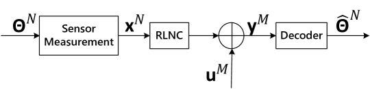
Figure 1: Block diagram for network compressive sensing model

Let $\mathsf{x}_{n}\in\mathbb{F}_{Q}$ be the measurement of $\mathsf{\Theta}_{n}$ obtained by the $n$-th sensor. The random vector $\boldsymbol{\mathsf{x}}^{N}=\left(\mathsf{x}_{1},\mathsf{x}_{2},\ldots,\mathsf{x}_{N}\right)\in\mathbb{F}_{Q}^{N}$ is a copy of the source vector $\boldsymbol{\mathsf{\Theta}}^{N}$ corrupted by the sensing noise. The sensing noise models the effect of imperfect measure acquisition at each sensor. It is described by the stationary transition probability $p_{\mathsf{x}\mid\mathsf{\Theta}}(x_{n}\mid\theta_{n})$, $\forall n$. Remark that this implies that $\boldsymbol{\mathsf{x}}^{N}$ is stationary as long as $\boldsymbol{\mathsf{\Theta}}^{N}$ is stationary. The local measurement $\mathsf{x}_{n}$ at node $n$ is used to compute a packet via RLNC [12], which is then broadcast and received by the neighbours of $n$. Each node in the network can act as a sink, and attempt reconstruction of $\boldsymbol{\mathsf{\Theta}}^{N}$, after a number $M\leq N$ of linear combinations has been received. The effects of RLNC at a sink node can be modeled as multiplying $\boldsymbol{\mathsf{x}}^{N}$ by a random matrix $\boldsymbol{\mathsf{A}}\in\mathbb{F}_{Q}^{M\times N}$. We assume that some communication noise $\boldsymbol{\mathsf{u}}^{M}\in\mathbb{F}_{Q}^{M}$ affects the received packets, modeling the effects of transmission. Each entry of $\boldsymbol{\mathsf{u}}^{M}$ is iid with pmf $p_{\mathsf{u}}\left(\cdot\right)$. The sink node is assumed to have received $M$ packets, with the $i$-th packet carrying the coefficients $\boldsymbol{\mathsf{A}}_{i}$ and the result of linear combination $\mathsf{y}_{i}\in\mathbb{F}_{Q}$, where $\boldsymbol{\mathsf{A}}_{i}$ is the $i$-th row of $\boldsymbol{\mathsf{A}}$ and $\mathsf{y}_{i}=\boldsymbol{\mathsf{A}}_{i}\boldsymbol{\mathsf{x}}^{N}+\mathsf{u}_{i}$, with all operations in $\mathbb{F}_{Q}$. The vector $\boldsymbol{\mathsf{y}}^{M}=\left(\mathsf{y}_{1},\mathsf{y}_{2},\ldots,\mathsf{y}_{M}\right)^{\textrm{t}}\in\mathbb{F}_{Q}^{M}$ can be then represented as

$$\boldsymbol{\mathsf{y}}^{M}=\boldsymbol{\mathsf{A}}\boldsymbol{\mathsf{x}}^{N}+\boldsymbol{\mathsf{u}}^{M},$$ (3)

where the network coding matrix $\boldsymbol{\mathsf{A}}$ plays the role of the random sensing matrix in the compressed sensing setup. According to the presence of the sensing and communication noises, one obtains four types of noise models, namely Without Noise (WN), Noise in Communications (NC) only, Noise in the Sensing process (NS) only, and noise in both Communications and in the Sensing process (NCS). These models are summarized in Table I.

Table I: Classification and notation based on the presence of noise

		Communication Noise
		absent	present
Sensing	absent	WN	NC
Noise	present	NS	NCS

In general, the matrix $\boldsymbol{\mathsf{A}}$ is not necessarily of full rank, and it is assumed to be independent of $\boldsymbol{\mathsf{x}}^{N}$. Two different assumptions about the structure of $\boldsymbol{\mathsf{A}}$ are considered here: (A1) the entries of $\boldsymbol{\mathsf{A}}$ are iid, uniformly distributed in $\mathbb{F}_{Q}$; (A2) the entries of $\boldsymbol{\mathsf{A}}$ are iid, all non-zero elements of $\mathbb{F}_{Q}$ are equiprobable. Both can be represented using the following model: for the entry $\mathsf{A}_{ij}$ of $\boldsymbol{\mathsf{A}}$,

$$\Pr\left(\mathsf{A}_{ij}=q\right)=\begin{cases}1-\gamma&q=0,\\ \gamma/\left(Q-1\right)&q\in\mathbb{F}_{Q}\setminus\left\{0\right\},\end{cases}$$ (4)

where $\gamma$ is the sparsity factor, $0<\gamma<1$, and $\boldsymbol{\mathsf{A}}$ is sparse if $\gamma<0.5$. We only assume that

$$0<\gamma\leq 1-Q^{-1}.$$ (5)

Notice that choosing $\gamma<1-Q^{-1}$ corresponds to assumption (A2), while choosing $\gamma=1-Q^{-1}$ corresponds to assumption (A1), since (4) becomes the uniform distribution.

In practice, sparse matrices are preferable. As the information of the sensing matrix is carried in the headers of packets [21, 22], the network coding overhead may be large if $\boldsymbol{\mathsf{A}}$ is dense and $N$ is large. Moreover, as mentioned in [14], sparse matrices facilitate the convergence of the approximate belief propagation algorithm [8]. In practice, the structure of $\boldsymbol{\mathsf{A}}$ is strongly dependent on the structure of the network. For example, [15] assumes that only a subset of sensors $\mathcal{S}{}_{i}\subset\mathcal{N}$ have participated in the $i$-th linear mixing. The content of the subsets $\mathcal{S}{}_{i}$ depends on the location of each sensor and is designed to minimize communication costs. In $\boldsymbol{\mathsf{A}}$, coefficients associated to nodes belonging to $\mathcal{S}{}_{i}$ follow a uniform distribution, while the others are null. This model, however, is not considered here, since we aim at a general asymptotic analysis, independent on the topology of the network.

II-C MAP Decoding

The sink node observes the realization $\mathbf{y}^{M}$ and perfectly knows the realization $\mathbf{A}$, e.g., from packet headers, see [21] and [22]. The maximum a posteriori estimate $\hat{\boldsymbol{\theta}}^{N}$ of the realization of $\boldsymbol{\mathsf{\Theta}}^{N}$ is evaluated as

$$\hat{\boldsymbol{\theta}}^{N}=\textrm{arg}\max_{\boldsymbol{\theta}^{N}\in\mathbb{F}_{Q}^{N}}p\left(\boldsymbol{\theta}^{N}\mid\mathbf{y}^{M},\mathbf{A}\right),$$ (6)

where the a posteriori pmf is

$$p\left(\boldsymbol{\theta}^{N}\mid\mathbf{y}^{M},\mathbf{A}\right) \propto p\left(\boldsymbol{\theta}^{N},\mathbf{y}^{M},\mathbf{A}\right)$$

$$=\sum_{\mathbf{x}^{N}\in\mathbb{F}_{Q}^{N}}\sum_{\mathbf{u}^{M}\in\mathbb{F}_{Q}^{M}}p\left(\boldsymbol{\theta}^{N},\mathbf{x}^{N},\mathbf{u}^{M},\mathbf{y}^{M},\mathbf{A}\right)$$

$$=\sum_{\mathbf{x}^{N}\in\mathbb{F}_{Q}^{N}}\sum_{\mathbf{u}^{M}\in\mathbb{F}_{Q}^{M}}p\left(\boldsymbol{\theta}^{N}\right)p\left(\mathbf{x}^{N}\mid\boldsymbol{\theta}^{N}\right)p\left(\mathbf{u}^{M}\right)p\left(\mathbf{A}\right)p\left(\mathbf{y}^{M}\mid\mathbf{x}^{N},\mathbf{u}^{M},\mathbf{A}\right).$$ (7)

Note that the conditional pmf $p\left(\mathbf{y}^{M}\mid\mathbf{x}^{N},\mathbf{u}^{M},\mathbf{A}\right)$ is an indicator function, i.e.,

$$p\left(\mathbf{y}^{M}\mid\mathbf{x}^{N},\mathbf{u}^{M},\mathbf{A}\right)=1_{\mathbf{y}^{M}=\mathbf{A}\mathbf{x}^{N}+\mathbf{u}^{M}}.$$ (8)

An error event (decoding error) occurs when $\hat{\boldsymbol{\theta}}^{N}\neq\boldsymbol{\theta}^{N}$, with probability

$$P_{\text{e}}=\Pr\left\{\hat{\boldsymbol{\mathsf{\Theta}}}^{N}\neq\boldsymbol{\mathsf{\Theta}}^{N}\right\}.$$ (9)

Our objective is to evaluate lower and upper bounds of (9) under MAP decoding, as functions of $M$, $N$, and $\gamma$, for the various source and noise models previously introduced. With these bounds, one can obtain necessary and sufficient conditions on the ratio $M/N$ for asymptotic (with $N\rightarrow\infty$) perfect recovery, i.e., to obtain

$$\lim_{N\rightarrow\infty}P_{\text{e}}=0.$$ (10)

III Necessary Condition for Asymptotic Perfect Recovery

This section derives the necessary conditions for asymptotically ($N\rightarrow\infty$) vanishing probability of decoding error. They only depend on the assumptions considered about the sensing and communication noises. We directly analyze the NCS case for the GSE source model. The results for this case can be easily adapted to the other cases. This work extends results obtained in [19] for the noiseless case (WN). Two situations are considered, depending on the value of the entropy rate

$$\mathcal{H}\left(\mathsf{x}\right)=\lim_{N\rightarrow\infty}\frac{1}{N}H\left(\boldsymbol{\mathsf{x}}^{N}\right).$$ (11)

Proposition 1 (Necessary condition for the NCS case).

Assume the presence of both communication and sensing noises and that $\mathcal{H}\left(\mathsf{x}\right)>0$. Consider some arbitrary small $\delta\in\mathbb{R}^{+}$. For $N\rightarrow\infty$, the necessary conditions for $P_{\text{e}}<\delta$ are

$$\mathcal{H}\left(\mathsf{\Theta},\mathsf{x}\right)-\mathcal{H}\left(\mathsf{x}\right)<3\varepsilon+\delta\log Q,$$ (12)

$$H\left(p_{\mathsf{u}}\right)<\log Q,$$ (13)

and

$$\frac{M}{N}>\frac{\mathcal{H}\left(\mathsf{\Theta},\mathsf{x}\right)-\left(5\varepsilon+2\delta\log Q\right)}{\log Q-H\left(p_{\mathsf{u}}\right)},$$ (14)

where $\varepsilon\in\mathbb{R}^{+}$ is an arbitrary small constant.

Corollary 1.

Consider the same hypotheses as in Proposition 1 and assume now that $\mathcal{H}\left(\mathsf{x}\right)=0$. Consider some arbitrary small $\delta\in\mathbb{R}^{+}$. For $N\rightarrow\infty$, the necessary condition for $P_{\text{e}}<\delta$ is

$$\mathcal{H}\left(\mathsf{\Theta},\mathsf{x}\right)<3\varepsilon+\delta\log Q,$$ (15)

where $\varepsilon\in\mathbb{R}^{+}$ is an arbitrary small constant.

In Proposition 1, (12) implies that for asymptotically exact recovery, $p\left(\boldsymbol{\mathsf{x}}^{N}\mid\boldsymbol{\mathsf{\Theta}}^{N}\right)$ should degenerate, almost surely, into a deterministic mapping. The condition (13) indicates that asymptotically exact recovery for non-deterministic sources is not possible in case of uniformly distributed communication noise. Finally, (14) indicates that the minimum number of required measurements depends both on the sensing and communication noises as well as on the distribution of $\mathsf{\Theta}$. In particular, for a given source with entropy rate $\mathcal{H}\left(\mathsf{\Theta}\right)$, the number of necessary measurements increases with the level of the sensing noise, determined by $\mathcal{H}\left(\mathsf{x}\mid\mathsf{\Theta}\right)$. Similarly, the number of necessary measurements increases when the communication noise gets closer to uniformly distributed. The following proof is inspired by the work in [19], with both communication noise and sensing noise are considered here.

Proof.

From the problem setup, one has the Markov chain

$$\boldsymbol{\mathsf{\Theta}}^{N}\leftrightarrow\boldsymbol{\mathsf{x}}^{N}\leftrightarrow\left(\boldsymbol{\mathsf{y}}^{M},\boldsymbol{\mathsf{A}}\right)\leftrightarrow\hat{\boldsymbol{\mathsf{\Theta}}}^{N},$$ (16)

from which one deduces that

$$H\left(\boldsymbol{\mathsf{\Theta}}^{N}\mid\boldsymbol{\mathsf{x}}^{N}\right)\leq H\left(\boldsymbol{\mathsf{\Theta}}^{N}\mid\hat{\boldsymbol{\mathsf{\Theta}}}^{N}\right),$$ (17)

and

$$H\left(\boldsymbol{\mathsf{x}}^{N}\mid\boldsymbol{\mathsf{y}}^{M},\boldsymbol{\mathsf{A}}\right)\leq H\left(\boldsymbol{\mathsf{\Theta}}^{N}\mid\hat{\boldsymbol{\mathsf{\Theta}}}^{N}\right).$$ (18)

Applying Fano’s inequality [23, Sec. 2.10], one gets

$$H\left(\boldsymbol{\mathsf{\Theta}}^{N}\mid\hat{\boldsymbol{\mathsf{\Theta}}}^{N}\right) \leq 1+P_{\text{e}}\cdot\log\left(Q^{N}-1\right)$$ (19)

$$< 1+NP_{\text{e}}\log Q,$$

an upper bound of $P_{\text{e}}$ is obtained combining (17) and (19),

$$P_{\text{e}}>\frac{H\left(\boldsymbol{\mathsf{\Theta}}^{N},\boldsymbol{\mathsf{x}}^{N}\right)-H\left(\boldsymbol{\mathsf{x}}^{N}\right)-1}{N\log Q}.$$ (20)

Since $\boldsymbol{\mathsf{\Theta}}^{N}$ and $\boldsymbol{\mathsf{x}}^{N}$ are stationary and ergodic, for any $\varepsilon>0$, there exists $N_{0}\in\mathbb{N}$ such that $\forall N>N_{0}$, one has

$$\begin{cases}\mathcal{H}\left(\mathsf{\Theta},\mathsf{x}\right)-\varepsilon<\frac{H\left(\boldsymbol{\mathsf{\Theta}}^{N},\boldsymbol{\mathsf{x}}^{N}\right)}{N}<\mathcal{H}\left(\mathsf{\Theta},\mathsf{x}\right)+\varepsilon,\\ \mathcal{H}\left(\mathsf{x}\right)-\varepsilon<\frac{H\left(\boldsymbol{\mathsf{x}}^{N}\right)}{N}<\mathcal{H}\left(\mathsf{x}\right)+\varepsilon,\\ \varepsilon>\frac{1}{N}.\end{cases}$$ (21)

Hence for $N>N_{0}$, (20) can be rewritten as

$$P_{\text{e}}>\frac{\mathcal{H}\left(\mathsf{\Theta},\mathsf{x}\right)-\mathcal{H}\left(\mathsf{x}\right)-3\varepsilon}{\log Q}.$$ (22)

For $P_{\text{e}}<\delta$, one deduces (12) from (22). For $\delta$ and $\varepsilon$ arbitrary small, (12) imposes $\mathcal{H}\left(\mathsf{\Theta},\mathsf{x}\right)=\mathcal{H}\left(\mathsf{x}\right)$, meaning that $\mathsf{\mathsf{\Theta}}$ should be deterministic knowing $\mathsf{x}$, almost surely.

From (18) and (19), one gets an other lower bound for $P_{\text{e}}$

$$P_{\text{e}}>\frac{H\left(\boldsymbol{\mathsf{x}}^{N}\mid\boldsymbol{\mathsf{y}}^{M},\boldsymbol{\mathsf{A}}\right)-1}{N\log Q}.$$ (23)

The conditional entropy $H\left(\boldsymbol{\mathsf{x}}^{N}\mid\boldsymbol{\mathsf{y}}^{M},\boldsymbol{\mathsf{A}}\right)$ can be bounded as

$$H\left(\boldsymbol{\mathsf{x}}^{N}\mid\boldsymbol{\mathsf{y}}^{M},\boldsymbol{\mathsf{A}}\right) = H\left(\boldsymbol{\mathsf{x}}^{N}\right)-I\left(\boldsymbol{\mathsf{x}}^{N};\boldsymbol{\mathsf{y}}^{M},\boldsymbol{\mathsf{A}}\right)$$ (24)

$$= H\left(\boldsymbol{\mathsf{x}}^{N}\right)-\left(I\left(\boldsymbol{\mathsf{x}}^{N};\boldsymbol{\mathsf{A}}\right)+I\left(\boldsymbol{\mathsf{x}}^{N};\boldsymbol{\mathsf{y}}^{M}\mid\boldsymbol{\mathsf{A}}\right)\right)$$

$$\overset{(a)}{=} H\left(\boldsymbol{\mathsf{x}}^{N}\right)-\left(H\left(\boldsymbol{\mathsf{y}}^{M}\mid\boldsymbol{\mathsf{A}}\right)-H\left(\boldsymbol{\mathsf{y}}^{M}\mid\boldsymbol{\mathsf{A}},\boldsymbol{\mathsf{x}}^{N}\right)\right)$$

$$\overset{(b)}{\geq} H\left(\boldsymbol{\mathsf{x}}^{N}\right)-M\cdot\log Q+H\left(\boldsymbol{\mathsf{y}}^{M}\mid\boldsymbol{\mathsf{A}},\boldsymbol{\mathsf{x}}^{N}\right)$$

$$\overset{(c)}{=} H\left(\boldsymbol{\mathsf{x}}^{N}\right)-M\cdot\log Q+MH\left(p_{\mathsf{u}}\right),$$

where $(a)$ follows from the assumption that $\boldsymbol{\mathsf{x}}^{N}$ and $\boldsymbol{\mathsf{A}}$ are independent, $(b)$ comes from $H\left(\boldsymbol{\mathsf{y}}^{M}\mid\boldsymbol{\mathsf{A}}\right)\leq H\left(\boldsymbol{\mathsf{y}}^{M}\right)\leq\log\left|\mathbb{F}_{Q}^{M}\right|=M\log Q$, and $(c)$ is because

$$H\left(\boldsymbol{\mathsf{y}}^{M}\mid\boldsymbol{\mathsf{A}},\boldsymbol{\mathsf{x}}^{N}\right)=H\left(\boldsymbol{\mathsf{A}}\boldsymbol{\mathsf{x}}^{N}+\boldsymbol{\mathsf{u}}^{M}\mid\boldsymbol{\mathsf{A}},\boldsymbol{\mathsf{x}}^{N}\right)=H\left(\boldsymbol{\mathsf{u}}^{M}\right)=MH\left(p_{\mathsf{u}}\right).$$ (25)

Using (23) and (24), a second necessary condition for $P_{\text{e}}<\delta$ is

$$\frac{H\left(\boldsymbol{\mathsf{x}}^{N}\right)-M\left(\log Q-H\left(p_{\mathsf{u}}\right)\right)-1}{N\log Q}<\delta.$$ (26)

For $N>N_{0}$, using (21) in (26) yields

$$\frac{\mathcal{H}\left(\mathsf{x}\right)-\frac{M}{N}\left(\log Q-H\left(p_{\mathsf{u}}\right)\right)-2\varepsilon}{\log Q}<\delta.$$ (27)

Now consider two cases. In the first case, the communication noise is assumed uniformly distributed, i.e.,

$$H\left(p_{\mathsf{u}}\right)=\log Q,$$ (28)

the condition (27) becomes

$$\mathcal{H}\left(\mathsf{x}\right)<\delta\log Q+2\varepsilon.$$ (29)

As $\delta$ can be made arbitrary small, (29) imposes that, for uniform communication noise, asymptotically vanishing probability of error is possible only if $\mathcal{H}\left(\mathsf{x}\right)$ is arbitrary close to zero. For non-degenerate cases, i.e., $\mathcal{H}\left(\mathsf{x}\right)>0$, one obtains the necessary condition (13). In this second case, a lower bound of the compression ratio $M/N$ is obtained immediately from (27),

$$\frac{M}{N}>\frac{\mathcal{H}\left(\mathsf{x}\right)-\left(2\varepsilon+\delta\log Q\right)}{\log Q-H\left(p_{\mathsf{u}}\right)}.$$ (30)

We can represent the condition (30) in terms of the joint entropy rate $\mathcal{H}\left(\mathsf{\Theta},\mathsf{x}\right)$ by applying (12). Then, one gets (14) and Proposition 1 is proved.

Consider now $\mathcal{H}\left(\mathsf{x}\right)=0$, then (27) holds for any value of $M/N$, and for any $H\left(p_{\mathsf{u}}\right)\leq\log Q$, since the left side of (27) is always negative. Hence, (12) is the only necessary condition for this case. Corollary 1 is also proved. ∎

With the results of the NCS noise model, one may derive the necessary conditions for the other models. If no sensing noise is considered, i.e., $\boldsymbol{\mathsf{x}}^{N}=\boldsymbol{\mathsf{\Theta}}^{N}$, one has $H\left(\boldsymbol{\mathsf{\Theta}}^{N}\mid\boldsymbol{\mathsf{x}}^{N}\right)=H\left(\boldsymbol{\mathsf{x}}^{N}\mid\boldsymbol{\mathsf{\Theta}}^{N}\right)=0$ and $H\left(\boldsymbol{\mathsf{\Theta}}^{N},\boldsymbol{\mathsf{x}}^{N}\right)=H\left(\boldsymbol{\mathsf{\Theta}}^{N}\right)$. If communication noise is absent, i.e., $\boldsymbol{\mathsf{u}}^{M}=\mathbf{0}$, $H\left(\boldsymbol{\mathsf{u}}^{M}\right)=0$. The necessary conditions for asymptotically ($N\rightarrow\infty$) vanishing probability of decoding error for each case are listed in Table 2.

Table II: Necessary conditions for asymptotic perfect recovery in noiseless and noisy cases

Case	Necessary Condition ($\mathcal{H}\left(\mathsf{x}\right)>0$)
WN	$\frac{M}{N}>\frac{\mathcal{H}\left(\mathsf{\Theta}\right)}{\log Q}$, already obtained in [19],
NC	$\frac{M}{N}>\frac{\mathcal{H}\left(\mathsf{\Theta}\right)}{\log Q-H\left(p_{\mathsf{u}}\right)}$ and $H\left(p_{\mathsf{u}}\right)<\log Q$,
NS	$\frac{M}{N}>\frac{\mathcal{H}\left(\mathsf{\Theta},\mathsf{x}\right)}{\log Q}$ and $\mathcal{H}\left(\mathsf{\Theta}\mid\mathsf{x}\right)=0$,
NCS	$\frac{M}{N}>\frac{\mathcal{H}\left(\mathsf{\Theta},\mathsf{x}\right)}{\log Q-H\left(p_{\mathsf{u}}\right)}$ and $H\left(p_{\mathsf{u}}\right)<\log Q$ and $\mathcal{H}\left(\mathsf{\Theta}\mid\mathsf{x}\right)=0$.

IV Sufficient Condition in Absence of Sensing Noise

This section provides an upper bound of the error probability for the MAP estimation problem in absence of sensing noise (the WN and NC cases). These two cases are considered simultaneously because their proofs are similar. When the channel noise vanishes, the NC case boils down to the WN case.

IV-A Upper Bound of the Error Probability

Proposition 2 (Upper bound of $P_{e}$, WN and NC cases).

Under MAP decoding, the asymptotic ($N\rightarrow\infty$) probability of error in absence of sensing noise can be upper bounded as

$$P_{\textrm{e}}\leq P_{1}\left(\alpha\right)+P_{2}\left(\alpha\right)+2\varepsilon,$$ (31)

where $\varepsilon\in\mathbb{R}^{+}$ is an arbitrarily small constant. $P_{1}\left(\alpha\right)$ and $P_{2}\left(\alpha\right)$ are defined as

$$P_{1}\left(\alpha\right)=2^{-N\left(-\frac{M}{N}\left(H\left(p_{\mathsf{u}}\right)+\log\left(1-\gamma\right)+\varepsilon\right)-H_{2}\left(\alpha\right)-\alpha\log\left(Q-1\right)-\frac{\log\left(\alpha N\right)}{N}\right)},$$ (32)

and

$$P_{2}\left(\alpha\right)=2^{-N\left(-\mathcal{H}\left(\mathsf{\mathsf{\Theta}}\right)-\frac{M}{N}\left(H\left(p_{\mathsf{u}}\right)+\log\left(Q^{-1}+\left(1-\frac{\gamma}{1-Q^{-1}}\right)^{\left\lceil\alpha N\right\rceil}\left(1-Q^{-1}\right)\right)+\varepsilon\right)-\varepsilon\right)},$$ (33)

with $\alpha\in\mathbb{R}^{+}$ and $\alpha<0.5$.

Proof.

The proof consists of two parts. First we define the error event, and then we analyze the probability of error.

Since no sensing noise is considered, we have $\boldsymbol{\mathsf{x}}^{N}=\boldsymbol{\mathsf{\Theta}}^{N}$ throughout this section. The a posteriori pmf (7) becomes

$$p\left(\boldsymbol{\theta}^{N}\mid\mathbf{y}^{M},\mathbf{A}\right)\propto\sum_{\mathbf{u}^{M}\in\mathbb{F}_{Q}^{M}}p\left(\boldsymbol{\theta}^{N}\right)p\left(\mathbf{u}^{M}\right)p\left(\mathbf{A}\right)1_{\mathbf{y}^{M}=\mathbf{A}\boldsymbol{\theta}^{N}+\mathbf{u}^{M}}.$$ (34)

Suppose that $\boldsymbol{\theta}^{N}$ (given but unknown) is the true state vector and consider that $\mathbf{A}$ has been generated randomly. At the sink, $\mathbf{A}$ and $\mathbf{y}^{M}$ are known. With MAP decoding, the reconstruction $\hat{\boldsymbol{\theta}}^{N}$ in (6) is

$$\hat{\boldsymbol{\theta}}^{N}=\textrm{arg}\max_{\boldsymbol{\theta}^{N}\in\mathbb{F}_{Q}^{N}}\sum_{\mathbf{u}^{M}\in\mathbb{F}_{Q}^{M}}p\left(\boldsymbol{\theta}^{N}\right)p\left(\mathbf{u}^{M}\right)p\left(\mathbf{A}\right)1_{\mathbf{y}^{M}=\mathbf{A}\boldsymbol{\theta}^{N}+\mathbf{u}^{M}}.$$ (35)

A decoding error happens if there exists a vector $\mathbf{\boldsymbol{\varphi}}^{N}\in\mathbb{F}_{Q}^{N}\setminus\left\{\boldsymbol{\theta}^{N}\right\}$ such that

$$\sum_{\mathbf{v}^{M}\in\mathbb{F}_{Q}^{M}}p\left(\mathbf{\boldsymbol{\varphi}}^{N}\right)p\left(\mathbf{v}^{M}\right)1_{\mathbf{y}^{M}=\mathbf{A}\mathbf{\boldsymbol{\varphi}}^{N}+\mathbf{v}^{M}}\geq\sum_{\mathbf{u}^{M}\in\mathbb{F}_{Q}^{M}}p\left(\boldsymbol{\theta}^{N}\right)p\left(\mathbf{u}^{M}\right)1_{\mathbf{y}^{M}=\mathbf{A}\boldsymbol{\theta}^{N}+\mathbf{u}^{M}}.$$ (36)

For fixed $\mathbf{y}^{M}$, $\mathbf{A}$, and $\boldsymbol{\theta}^{N}$, there is exactly one vector $\mathbf{u}^{M}$ such that $\mathbf{u}^{M}=\mathbf{y}^{M}-\mathbf{A}\boldsymbol{\theta}^{N}$. Hence the right side of (36) can be represented as $p_{\boldsymbol{\mathsf{\Theta}}^{N}}\left(\boldsymbol{\theta}^{N}\right)p_{\boldsymbol{\mathsf{u}}^{M}}\left(\mathbf{y}^{M}-\mathbf{A}\boldsymbol{\theta}^{N}\right)$. The subscripts for the pmfs are introduced to avoid any ambiguity of notations. Then (36) is equivalent to

$$p_{\boldsymbol{\mathsf{\Theta}}^{N}}\left(\mathbf{\boldsymbol{\varphi}}^{N}\right)p_{\boldsymbol{\mathsf{u}}^{M}}\left(\mathbf{y}^{M}-\mathbf{A}\mathbf{\boldsymbol{\varphi}}^{N}\right)\geq p_{\boldsymbol{\mathsf{\Theta}}^{N}}\left(\boldsymbol{\theta}^{N}\right)p_{\boldsymbol{\mathsf{u}}^{M}}\left(\mathbf{y}^{M}-\mathbf{A}\boldsymbol{\theta}^{N}\right).$$ (37)

An alternative way to state the error event can be: For a given realization $\boldsymbol{\mathsf{\Theta}}^{N}=\boldsymbol{\theta}^{N}$, which implies the realization $\boldsymbol{\mathsf{u}}^{M}=\mathbf{u}^{M}=\mathbf{y}^{M}-\mathbf{A}\boldsymbol{\theta}^{N}$, there exists a pair $(\mathbf{\boldsymbol{\varphi}}^{N},\mathbf{v}^{M})\in\mathbb{F}_{Q}^{N}\times\mathbb{F}_{Q}^{M}$ such that

$$\begin{cases}\mathbf{\boldsymbol{\varphi}}^{N}\neq\boldsymbol{\theta}^{N},\\ \mathbf{A}\mathbf{\boldsymbol{\varphi}}^{N}+\mathbf{v}^{M}=\mathbf{y}^{M}=\mathbf{A}\boldsymbol{\theta}^{N}+\mathbf{u}^{M},\\ p\left(\mathbf{\boldsymbol{\varphi}}^{N}\right)p\left(\mathbf{v}^{M}\right)\geq p\left(\boldsymbol{\theta}^{N}\right)p\left(\mathbf{u}^{M}\right).\end{cases}$$ (38)

From conditions (38), one concludes that the MAP decoder is equivalent to the maximum $Q$-probability decoder [24] in the NC case.

An upper bound of the error probability is now derived. For a fixed $\boldsymbol{\theta}^{N}$ and $\mathbf{u}^{M}$, the conditional error probability is denoted by $\Pr\left\{\textrm{error}\mid\boldsymbol{\theta}^{N},\mathbf{u}^{M}\right\}$. The average error probability is

$$P_{\textrm{e}}=\sum_{\boldsymbol{\theta}^{N}\in\mathbb{F}_{Q}^{N}}\sum_{\mathbf{u}^{M}\in\mathbb{F}_{Q}^{M}}p\left(\boldsymbol{\theta}^{N},\mathbf{u}^{M}\right)\Pr\left\{\textrm{error}\mid\boldsymbol{\theta}^{N},\mathbf{u}^{M}\right\}.$$ (39)

Weak typicality is instrumental in the following proofs. The notations of [25, Definition 4.2] are extended to stationary and ergodic sources. For any positive real number $\varepsilon$ and some integer $N>0$, the weakly typical set $\mathcal{A}_{\left[\mathsf{\Theta}\right]\varepsilon}^{N}\subset\mathbb{F}_{Q}^{N}$ for a stationary and ergodic source $\boldsymbol{\mathsf{\Theta}}^{N}$ is the set of vectors $\boldsymbol{\theta}^{N}\in\mathbb{F}_{Q}^{N}$ satisfying

$$\left|-\frac{1}{N}\log p\left(\boldsymbol{\theta}^{N}\right)-\mathcal{H}\left(\mathsf{\mathsf{\Theta}}\right)\right|\leq\varepsilon,$$ (40)

where $\mathcal{H}\left(\mathsf{\mathsf{\Theta}}\right)$ is the entropy rate of the source. Similarly, for the noise vector $\boldsymbol{\mathsf{u}}^{M}$, define

$$\mathcal{A}_{\left[\mathsf{u}\right]\varepsilon}^{M}=\left\{\mathbf{u}^{M}\in\mathbb{F}_{Q}^{M}:\>\left|-\frac{1}{M}\log p\left(\mathbf{u}^{M}\right)-H\left(p_{\mathsf{u}}\right)\right|\leq\varepsilon\right\}.$$ (41)

Recall that the entries of $\boldsymbol{\mathsf{u}}^{M}$ are uncorrelated, so $\mathcal{H}\left(\mathsf{u}\right)=H\left(p_{\mathsf{u}}\right)$. Thanks to Shannon-McMillan-Breiman theorem [23, Sec. 16.8], the pmf of the general stationary and ergodic source converges. In other words, for any $\varepsilon>0$, there exists $N_{\varepsilon}$ and $M_{\varepsilon}$ such that for all $N>N_{\varepsilon}$ and $M>M_{\varepsilon}$,

$$\Pr\left\{\left|-\frac{1}{N}\log p\left(\boldsymbol{\mathsf{\Theta}}^{N}\right)-\mathcal{H}\left(\mathsf{\Theta}\right)\right|\leq\varepsilon\right\}\geq 1-\varepsilon,$$ (42)

and

$$\Pr\left\{\left|-\frac{1}{M}\log p\left(\boldsymbol{\mathsf{u}}^{M}\right)-\mathcal{H}\left(p_{\mathsf{u}}\right)\right|\leq\varepsilon\right\}\geq 1-\varepsilon.$$ (43)

We can make $\varepsilon$ arbitrary close to zero as $N\rightarrow\infty$ and $M\rightarrow\infty$. A sandwich proof of this theorem is proposed in [23, Sec. 16.8]. For the sparse and uncorrelated source as defined in (1), $\mathcal{H}\left(\mathsf{\Theta}\right)$ is equal to $H\left(p_{\mathsf{\Theta}}\right)$, the entropy of a single source. The entropy rate of the StM source is the conditional entropy $H\left(\mathsf{\Theta}_{n+r}\mid\mathbf{\boldsymbol{\mathsf{\Theta}}}_{n}^{n+r-1}\right)$.

From (42) and (43), one has $\Pr\left\{\boldsymbol{\mathsf{\Theta}}^{N}\in\mathcal{A}_{\left[\mathsf{\Theta}\right]\varepsilon}^{N}\right\}\geq 1-\varepsilon$ and $\Pr\left\{\boldsymbol{\mathsf{u}}^{M}\in\mathcal{A}_{\left[\mathsf{u}\right]\varepsilon}^{M}\right\}\geq 1-\varepsilon$ for $N>N_{\varepsilon}$ and $M>M_{\varepsilon}$. It implies that, for $N$ and $M$ sufficiently large, $\boldsymbol{\mathsf{\Theta}}^{N}$ and $\boldsymbol{\mathsf{u}}^{M}$ belong to the weakly typical set $\mathcal{A}_{\left[\mathsf{\Theta}\right]\varepsilon}^{N}$ and $\mathcal{A}_{\left[\mathsf{u}\right]\varepsilon}^{M}$, almost surely. With respect to the typicality, $\mathbb{F}_{Q}^{N}\times\mathbb{F}_{Q}^{M}$ can be divided into two parts. Define the sets $\mathcal{U}$ and $\mathcal{U}^{\textrm{c}}$ for the pair of vectors $\left(\boldsymbol{\theta}^{N},\mathbf{u}^{M}\right)$, such that $\mathcal{U}\cup\mathcal{U}^{\textrm{c}}=\mathbb{F}_{Q}^{N}\times\mathbb{F}_{Q}^{M}$ and

$$\mathcal{U}=\left\{\boldsymbol{\theta}^{N}\in\mathbb{F}_{Q}^{N},\>\mathbf{u}^{M}\in\mathbb{F}_{Q}^{M}:\>\boldsymbol{\theta}^{N}\in\mathcal{A}_{\left[\mathsf{\Theta}\right]\varepsilon}^{N}\textrm{ and }\mathbf{u}^{M}\in\mathcal{A}_{\left[\mathsf{u}\right]\varepsilon}^{M}\right\},$$ (44)

$$\mathcal{U}^{\textrm{c}}=\left\{\boldsymbol{\theta}^{N}\in\mathbb{F}_{Q}^{N},\>\mathbf{u}^{M}\in\mathbb{F}_{Q}^{M}:\>\boldsymbol{\theta}^{N}\notin\mathcal{A}_{\left[\mathsf{\Theta}\right]\varepsilon}^{N}\textrm{ or }\mathbf{u}^{M}\notin\mathcal{A}_{\left[\mathsf{u}\right]\varepsilon}^{M}\right\}.$$ (45)

$\mathcal{U}$ is the joint typical set for $(\boldsymbol{\theta}^{N},\mathbf{u}^{M})$, due to the independence of $\boldsymbol{\mathsf{\Theta}}^{N}$ and $\boldsymbol{\mathsf{u}}^{M}$. The error probability can be bounded as

$$P_{\textrm{e}} = \sum_{\left(\boldsymbol{\theta}^{N},\mathbf{u}^{M}\right)\in\mathcal{U}}p\left(\boldsymbol{\theta}^{N}\right)p\left(\mathbf{u}^{M}\right)\cdot\Pr\left\{\textrm{error}\mid\boldsymbol{\theta}^{N},\mathbf{u}^{M}\right\}$$ (46)

$$+\sum_{\left(\boldsymbol{\theta}^{N},\mathbf{u}^{M}\right)\in\mathcal{U}^{\textrm{c}}}p\left(\boldsymbol{\theta}^{N}\right)p\left(\mathbf{u}^{M}\right)\cdot\Pr\left\{\textrm{error}\mid\boldsymbol{\theta}^{N},\mathbf{u}^{M}\right\}$$

$$\overset{(a)}{\leq} \sum_{\left(\boldsymbol{\theta}^{N},\mathbf{u}^{M}\right)\in\mathcal{U}}p\left(\boldsymbol{\theta}^{N}\right)p\left(\mathbf{u}^{M}\right)\cdot\Pr\left\{\textrm{error}\mid\boldsymbol{\theta}^{N},\mathbf{u}^{M}\right\}+\sum_{\left(\boldsymbol{\theta}^{N},\mathbf{u}^{M}\right)\in\mathcal{U}^{\textrm{c}}}p\left(\boldsymbol{\theta}^{N}\right)p\left(\mathbf{u}^{M}\right)$$

$$\overset{(b)}{\leq} \sum_{\left(\boldsymbol{\theta}^{N},\mathbf{u}^{M}\right)\in\mathcal{U}}p\left(\boldsymbol{\theta}^{N}\right)p\left(\mathbf{u}^{M}\right)\cdot\Pr\left\{\textrm{error}\mid\boldsymbol{\theta}^{N},\mathbf{u}^{M}\right\}+2\varepsilon,$$

where $(a)$ comes from $\Pr\left(\textrm{error}\mid\boldsymbol{\theta}^{N},\mathbf{u}^{M}\right)\leq 1$ and $(b)$ follows from the fact that

$$\sum_{\left(\boldsymbol{\theta}^{N},\mathbf{u}^{M}\right)\in\mathcal{U}^{\textrm{c}}}p\left(\boldsymbol{\theta}^{N}\right)p\left(\mathbf{u}^{M}\right) = 1-\sum_{\left(\boldsymbol{\theta}^{N},\mathbf{u}^{M}\right)\in\mathcal{U}}p\left(\boldsymbol{\theta}^{N}\right)p\left(\mathbf{u}^{M}\right)$$ (47)

$$= 1-\sum_{\boldsymbol{\theta}^{N}\in\mathcal{A}_{\left[\mathsf{\Theta}\right]\varepsilon}^{N}}p\left(\boldsymbol{\theta}^{N}\right)\sum_{\mathbf{u}^{M}\in\mathcal{A}_{\left[\mathsf{u}\right]\varepsilon}^{M}}p\left(\mathbf{u}^{M}\right)$$

$$\leq 1-\left(1-\varepsilon\right)\left(1-\varepsilon\right)\leq 2\varepsilon.$$

Since $\mathbb{A}$ is generated randomly, define the random event

$$\mathcal{E}\left(\boldsymbol{\theta}^{N},\mathbf{u}^{M};\mathbf{\boldsymbol{\varphi}}^{N},\mathbf{v}^{M}\right)=\left\{\boldsymbol{\mathsf{A}}\boldsymbol{\theta}^{N}+\mathbf{u}^{M}=\boldsymbol{\mathsf{A}}\mathbf{\boldsymbol{\varphi}}^{N}+\mathbf{v}^{M}\right\},$$ (48)

where $\left(\boldsymbol{\theta}^{N},\mathbf{u}^{M}\right)$ is the realization of the environment state, and $(\mathbf{\boldsymbol{\varphi}}^{N},\mathbf{v}^{M})$ is the potential reconstruction result. Conditioned on $\left(\boldsymbol{\theta}^{N},\mathbf{u}^{M}\right)$, $\Pr\left\{\textrm{error}\mid\boldsymbol{\theta}^{N},\mathbf{u}^{M}\right\}$ is in fact the probability of the union of the events $\mathcal{E}\left(\boldsymbol{\theta}^{N},\mathbf{u}^{M};\mathbf{\boldsymbol{\varphi}}^{N},\mathbf{v}^{M}\right)$ with all the parameter pairs $(\mathbf{\boldsymbol{\varphi}}^{N},\mathbf{v}^{M})\in\mathbb{F}_{Q}^{N}\times\mathbb{F}_{Q}^{M}$ such that $\mathbf{\boldsymbol{\varphi}}^{N}\neq\boldsymbol{\theta}^{N}$ and $p\left(\mathbf{\boldsymbol{\varphi}}^{N}\right)p\left(\mathbf{v}^{M}\right)\geq p\left(\boldsymbol{\theta}^{N}\right)p\left(\mathbf{u}^{M}\right)$, see (38). The conditional error probability can then be rewritten as

$$\Pr\left\{\textrm{error}\mid\boldsymbol{\theta}^{N},\mathbf{u}^{M}\right\}=\Pr\left\{\underset{{}_{p\left(\mathbf{\boldsymbol{\varphi}}^{N}\right)p\left(\mathbf{v}^{M}\right)\geq p\left(\boldsymbol{\theta}^{N}\right)p\left(\mathbf{u}^{M}\right)}^{\>\mathbf{\boldsymbol{\varphi}}^{N}\in\mathbb{F}_{Q}^{N}\setminus\left\{\boldsymbol{\theta}^{N}\right\},\>\mathbf{v}^{M}\in\mathbb{F}_{Q}^{M}:}}{\bigcup}\mathcal{E}\left(\boldsymbol{\theta}^{N},\mathbf{u}^{M};\mathbf{\boldsymbol{\varphi}}^{N},\mathbf{v}^{M}\right)\right\}.$$ (49)

Introducing (49) in (46) and applying the union bound yields

$$P_{\textrm{e}} \leq \sum_{\left(\boldsymbol{\theta}^{N},\mathbf{u}^{M}\right)\in\mathcal{U}}p\left(\boldsymbol{\theta}^{N}\right)p\left(\mathbf{u}^{M}\right)\underset{{}_{p\left(\mathbf{\boldsymbol{\varphi}}^{N}\right)p\left(\mathbf{v}^{M}\right)\geq p\left(\boldsymbol{\theta}^{N}\right)p\left(\mathbf{u}^{M}\right)}^{\>\mathbf{\boldsymbol{\varphi}}^{N}\in\mathbb{F}_{Q}^{N}\setminus\left\{\boldsymbol{\theta}^{N}\right\},\>\mathbf{v}^{M}\in\mathbb{F}_{Q}^{M}:}}{\sum}\Pr\left\{\mathcal{E}\left(\boldsymbol{\theta}^{N},\mathbf{u}^{M};\mathbf{\boldsymbol{\varphi}}^{N},\mathbf{v}^{M}\right)\right\}+2\varepsilon$$ (50)

$$= \sum_{\left(\boldsymbol{\theta}^{N},\mathbf{u}^{M}\right)\in\mathcal{U}}p\left(\boldsymbol{\theta}^{N}\right)p\left(\mathbf{u}^{M}\right)$$

$$\cdot\underset{{}_{\quad\mathbf{v}^{M}\in\mathbb{F}_{Q}^{M}}^{\mathbf{\boldsymbol{\varphi}}^{N}\in\mathbb{F}_{Q}^{N}\setminus\left\{\boldsymbol{\theta}^{N}\right\}}}{\sum}\Phi\left(\boldsymbol{\theta}^{N},\mathbf{u}^{M};\mathbf{\boldsymbol{\varphi}}^{N},\mathbf{v}^{M}\right)\Pr\left\{\mathcal{E}\left(\boldsymbol{\theta}^{N},\mathbf{u}^{M};\mathbf{\boldsymbol{\varphi}}^{N},\mathbf{v}^{M}\right)\right\}+2\varepsilon,$$

where

$$\Phi\left(\boldsymbol{\theta}^{N},\mathbf{u}^{M};\mathbf{\boldsymbol{\varphi}}^{N},\mathbf{v}^{M}\right)=\begin{cases}1&\textrm{ if }p\left(\mathbf{\boldsymbol{\varphi}}^{N}\right)p\left(\mathbf{v}^{M}\right)\geq p\left(\boldsymbol{\theta}^{N}\right)p\left(\mathbf{u}^{M}\right),\\ 0&\textrm{ if }p\left(\mathbf{\boldsymbol{\varphi}}^{N}\right)p\left(\mathbf{v}^{M}\right)<p\left(\boldsymbol{\theta}^{N}\right)p\left(\mathbf{u}^{M}\right).\end{cases}$$ (51)

Now consider the following lemma.

Lemma 1 (Upper bound of $\Phi$). Consider some $s\in\mathbb{R}^{+}$ with $s\leq 1$. For any $\boldsymbol{\theta}^{N},\mathbf{\boldsymbol{\varphi}}^{N}$ in $\mathbb{F}_{Q}^{N}$ and $\mathbf{u}^{M},\mathbf{v}^{M}$ in $\mathbb{F}_{Q}^{M}$, the following inequality holds,

$$\Phi\left(\boldsymbol{\theta}^{N},\mathbf{\boldsymbol{\varphi}}^{N},\mathbf{u}^{M},\mathbf{v}^{M}\right)\leq\left(\frac{p\left(\mathbf{\boldsymbol{\varphi}}^{N}\right)p\left(\mathbf{v}^{M}\right)}{p\left(\boldsymbol{\theta}^{N}\right)p\left(\mathbf{u}^{M}\right)}\right)^{s}.$$ (52)

Lemma 1 is a part of Gallager’s derivation of error exponents in [26, Sec. 5.6]. Introducing (52) with $s=1$ into (50), one gets

$$P_{\textrm{e}}\leq\sum_{\left(\boldsymbol{\theta}^{N},\mathbf{u}^{M}\right)\in\mathcal{U}}\underset{{}_{\quad\mathbf{v}^{M}\in\mathbb{F}_{Q}^{M}}^{\mathbf{\boldsymbol{\varphi}}^{N}\in\mathbb{F}_{Q}^{N}\setminus\left\{\boldsymbol{\theta}^{N}\right\}}}{\sum}p\left(\mathbf{\boldsymbol{\varphi}}^{N}\right)p\left(\mathbf{v}^{M}\right)\Pr\left\{\mathcal{E}\left(\boldsymbol{\theta}^{N},\mathbf{u}^{M};\mathbf{\boldsymbol{\varphi}}^{N},\mathbf{v}^{M}\right)\right\}+2\varepsilon.$$ (53)

In (53),

$$\Pr\left\{\mathcal{E}\left(\boldsymbol{\theta}^{N},\mathbf{u}^{M};\mathbf{\boldsymbol{\varphi}}^{N},\mathbf{v}^{M}\right)\right\}=\Pr\left\{\boldsymbol{\mathsf{A}}\mathbf{\boldsymbol{\mu}}^{N}=\mathbf{s}^{M}\mid\mathbf{\boldsymbol{\mu}}^{N}\neq\mathbf{0},\mathbf{s}^{M}\right\}$$ (54)

with $\mathbf{\boldsymbol{\mu}}^{N}=\mathbf{\boldsymbol{\varphi}}^{N}-\boldsymbol{\theta}^{N}\in\mathbb{F}_{Q}^{N}\setminus\left\{\mathbf{0}\right\}$, and $\mathbf{s}^{M}=\mathbf{v}^{M}-\mathbf{u}^{M}\in\mathbb{F}_{Q}^{M}$. This probability depends on the sparsity of $\mathbf{\boldsymbol{\mu}}^{N}$ and of $\mathbf{s}^{M}$, let $d_{1}=\left\|\mathbf{\boldsymbol{\mu}}^{N}\right\|_{0}$ and $d_{2}=\left\|\mathbf{s}^{M}\right\|_{0}$. Both $d_{1}$ and $d_{2}$ are integers such that $1\leq d_{1}\leq N$ and $0\leq d_{2}\leq M$. Define the multivariable function

$$f\left(d_{1},d_{2};\gamma,Q,M\right)=\Pr\left\{\boldsymbol{\mathsf{A}}\mathbf{\boldsymbol{\mu}}^{N}=\mathbf{s}^{M}\mid\left\|\mathbf{\boldsymbol{\mu}}^{N}\right\|_{0}=d_{1},\left\|\mathbf{s}^{M}\right\|_{0}=d_{2}\right\},$$ (55)

where $\gamma$, $Q$, and $M$ are the parameters of the random matrix $\boldsymbol{\mathsf{A}}$.

$$\Pr\left\{\boldsymbol{\mathsf{A}}\mathbf{\boldsymbol{\mu}}^{N}=\mathbf{0}\mid\mathbf{\boldsymbol{\mu}}^{N}\neq\mathbf{0}\right\}=f\left(d_{1},0;\gamma,Q,M\right)$$

has been evaluated in [27] and [19]. We provide a simple extension of this result for $d_{2}\neq 0$.

Lemma 2 (Properties of $f\left(d_{1},d_{2};\gamma,Q,M\right)$). The function $f\left(d_{1},d_{2};\gamma,Q,M\right)$, defined in (55), is non-increasing in $d_{2}$ for a given $d_{1}$ and

$$f\left(d_{1},d_{2};\gamma,Q,M\right)\leq f\left(d_{1},0;\gamma,Q,M\right)=\left(Q^{-1}+\left(1-\frac{\gamma}{1-Q^{-1}}\right)^{d_{1}}\left(1-Q^{-1}\right)\right)^{M}.$$ (56)

Moreover $f\left(d_{1},0;\gamma,Q,M\right)$ is non-increasing in $d_{1}$ and

$$f\left(d_{1},0;\gamma,Q,M\right)\leq f\left(1,0;\gamma,Q,M\right)=\left(1-\gamma\right)^{M}.$$ (57)

If $\gamma=1-Q^{-1}$, which corresponds to a uniformly distributed sensing matrix,

$$f\left(d_{1},d_{2};\gamma,Q,M\right)=Q^{-M}$$ (58)

is constant.

See Appendix A for the proof details. Using Lemma 2, (53) can be expressed as

$$P_{\textrm{e}} \overset{(a)}{\leq} \sum_{d_{1}=1}^{N}\sum_{d_{2}=0}^{M}\underset{{}_{\mathbf{v}^{M}\in\mathbb{F}_{Q}^{M}:\left\|\mathbf{u}^{M}-\mathbf{v}^{M}\right\|_{0}=d_{2}}^{{}_{\,\mathbf{\boldsymbol{\varphi}}^{N}\in\mathbb{F}_{Q}^{N}:\left\|\mathbf{\boldsymbol{\varphi}}^{N}-\boldsymbol{\theta}^{N}\right\|_{0}=d_{1}}^{\qquad\left(\boldsymbol{\theta}^{N},\mathbf{u}^{M}\right)\in\mathcal{U}}}}{\sum}p\left(\mathbf{\boldsymbol{\varphi}}^{N}\right)p\left(\mathbf{v}^{M}\right)f\left(d_{1},d_{2};\gamma,Q,M\right)+2\varepsilon$$ (59)

$$\overset{(b)}{\leq} \sum_{d_{1}=1}^{N}\underset{{}^{{}_{\mathbf{\boldsymbol{\varphi}}^{N}\in\mathbb{F}_{Q}^{N}:\left\|\mathbf{\boldsymbol{\varphi}}^{N}-\boldsymbol{\theta}^{N}\right\|_{0}=d_{1}}^{\qquad\left(\boldsymbol{\theta}^{N},\mathbf{u}^{M}\right)\in\mathcal{U}}}}{\sum}p\left(\mathbf{\boldsymbol{\varphi}}^{N}\right)f\left(d_{1},0;\gamma,Q,M\right)\left(\sum_{\mathbf{v}^{M}\in\mathbb{F}_{Q}^{M}}p\left(\mathbf{v}^{M}\right)\right)+2\varepsilon$$

$$\overset{(c)}{\leq} \sum_{d_{1}=1}^{\left\lfloor\alpha N\right\rfloor}\underset{{}^{{}_{\mathbf{\boldsymbol{\varphi}}^{N}\in\mathbb{F}_{Q}^{N}:\left\|\mathbf{\boldsymbol{\varphi}}^{N}-\boldsymbol{\theta}^{N}\right\|_{0}=d_{1}}^{\qquad\left(\boldsymbol{\theta}^{N},\mathbf{u}^{M}\right)\in\mathcal{U}}}}{\sum}p\left(\mathbf{\boldsymbol{\varphi}}^{N}\right)f\left(1,0;\gamma,Q,M\right)$$

$$+\sum_{d_{1}=\left\lceil\alpha N\right\rceil}^{N}\underset{{}^{{}_{\mathbf{\boldsymbol{\varphi}}^{N}\in\mathbb{F}_{Q}^{N}:\left\|\mathbf{\boldsymbol{\varphi}}^{N}-\boldsymbol{\theta}^{N}\right\|_{0}=d_{1}}^{\qquad\left(\boldsymbol{\theta}^{N},\mathbf{u}^{M}\right)\in\mathcal{U}}}}{\sum}p\left(\mathbf{\boldsymbol{\varphi}}^{N}\right)f\left(\left\lceil\alpha N\right\rceil,0;\gamma,Q,M\right)+2\varepsilon,$$

where $(a)$ is by the classification of $\mathbf{\boldsymbol{\varphi}}^{N}$ and $\mathbf{v}^{M}$ according to the $\ell_{0}$ norm of their difference with $\boldsymbol{\theta}^{N}$ and $\mathbf{u}^{M}$ respectively and $(b)$ is obtained using the bound (56) and using $\sum_{\mathbf{v}^{M}\in\mathbb{F}_{Q}^{M}}p\left(\mathbf{v}^{M}\right)=1$. The splitting in $(c)$ permits $f\left(d_{1},0;\gamma,Q,M\right)$ to be bounded in different cases, this idea comes from [27] and is also meaningful here. The parameter $\alpha$ is a positive real number with $0<\alpha<0.5$. The way to choose $\alpha$ is discussed in Section IV-B. The two terms in (59), denoted by $P_{\mathcal{U}_{1}}\left(\alpha\right)$ and $P_{\mathcal{U}_{2}}\left(\alpha\right)$, need to be considered separately. For the first term $P_{\mathcal{U}_{1}}\left(\alpha\right)$, we have

$$P_{\mathcal{U}_{1}}\left(\alpha\right) = f\left(1,0;\gamma,Q,M\right)\sum_{d_{1}=1}^{\left\lfloor\alpha N\right\rfloor}\underset{{}^{{}_{\mathbf{\boldsymbol{\varphi}}^{N}\in\mathbb{F}_{Q}^{N}:\left\|\mathbf{\boldsymbol{\varphi}}^{N}-\boldsymbol{\theta}^{N}\right\|_{0}=d_{1}}^{\qquad\left(\boldsymbol{\theta}^{N},\mathbf{u}^{M}\right)\in\mathcal{U}}}}{\sum}p\left(\mathbf{\boldsymbol{\varphi}}^{N}\right)$$ (60)

$$\overset{(a)}{=} \left(1-\gamma\right)^{M}\sum_{\mathbf{u}^{M}\in\mathcal{A}_{\left[\mathsf{u}\right]\varepsilon}^{M}}\sum_{d_{1}=1}^{\left\lfloor\alpha N\right\rfloor}\sum_{\mathbf{\boldsymbol{\varphi}}^{N}\in\mathbb{F}_{Q}^{N}}p\left(\mathbf{\boldsymbol{\varphi}}^{N}\right)\underset{{}^{{}_{\left\|\boldsymbol{\theta}^{N}-\mathbf{\boldsymbol{\varphi}}^{N}\right\|_{0}=d_{1}}^{\quad\boldsymbol{\theta}^{N}\in\mathcal{A}_{\left[\mathsf{\Theta}\right]\varepsilon}^{N}:}}}{\sum}1$$

$$\overset{(b)}{\leq} \left(1-\gamma\right)^{M}\sum_{\mathbf{u}^{M}\in\mathcal{A}_{\left[\mathsf{u}\right]\varepsilon}^{M}}\sum_{d_{1}=1}^{\left\lfloor\alpha N\right\rfloor}\sum_{\mathbf{\boldsymbol{\varphi}}^{N}\in\mathbb{F}_{Q}^{N}}p\left(\mathbf{\boldsymbol{\varphi}}^{N}\right)\left|\left\{\boldsymbol{\theta}^{N}\in\mathbb{F}_{Q}^{N}:\left\|\boldsymbol{\theta}^{N}-\mathbf{\boldsymbol{\varphi}}^{N}\right\|_{0}=d_{1}\right\}\right|$$

$$\overset{(c)}{\leq} \left(1-\gamma\right)^{M}\sum_{\mathbf{u}^{M}\in\mathcal{A}_{\left[\mathsf{u}\right]\varepsilon}^{M}}\sum_{d_{1}=1}^{\left\lfloor\alpha N\right\rfloor}2^{NH_{2}\left(\frac{d_{1}}{N}\right)}\left(Q-1\right)^{d_{1}}$$

$$\overset{(d)}{\leq} \left(1-\gamma\right)^{M}\cdot\left|\mathcal{A}_{\left[\mathsf{u}\right]\varepsilon}^{M}\right|\cdot\alpha N\cdot 2^{NH_{2}\left(\alpha\right)}\left(Q-1\right)^{\alpha N}$$

$$\overset{(e)}{\leq} 2^{-N\left(-\frac{M}{N}\left(H\left(p_{\mathsf{u}}\right)+\log\left(1-\gamma\right)+\varepsilon\right)-H_{2}\left(\alpha\right)-\alpha\log\left(Q-1\right)-\frac{\log\left(\alpha N\right)}{N}\right)}=P_{1}\left(\alpha\right)$$

where $(a)$ is by changing the order of summation and $(b)$ is obtained considering all $\boldsymbol{\theta}^{N}\in\mathbb{F}_{Q}^{N}$ and not only typical sequences. The bound $(c)$ is obtained noticing that

$$\left|\left\{\boldsymbol{\theta}^{N}\in\mathbb{F}_{Q}^{N}:\left\|\boldsymbol{\theta}^{N}-\mathbf{\boldsymbol{\varphi}}^{N}\right\|_{0}=d_{1}\right\}\right| = \left({}_{d_{1}}^{N}\right)\left(Q-1\right)^{d_{1}}$$ (61)

$$\leq 2^{NH_{2}\left(\frac{d_{1}}{N}\right)}\left(Q-1\right)^{d_{1}},$$

where $H_{2}\left(p\right)$ denotes the entropy of a Bernoulli-$p$ source and $\sum_{\mathbf{\boldsymbol{\varphi}}^{N}\in\mathbb{F}_{Q}^{N}}p\left(\mathbf{\boldsymbol{\varphi}}^{N}\right)=1$; $(d)$ is because of the monotonicity of the function $H_{2}\left(\frac{d_{1}}{N}\right)$, which is increasing in $d_{1}$ as $d_{1}\leq\left\lfloor\alpha N\right\rfloor<N/2$; $\left(e\right)$ comes from [23, Theorem 3.1.2], the upper bound of the size of $\mathcal{A}_{\left[\mathsf{u}\right]\varepsilon}^{M}$, i.e.,

$$\left|\mathcal{A}_{\left[\mathsf{u}\right]\varepsilon}^{M}\right|\leq 2^{M\left(H\left(p_{\mathsf{u}}\right)+\varepsilon\right)},$$ (62)

for $M>M_{\varepsilon}$. Similarly, for $N>N_{\varepsilon}$, one has

$$\left|\mathcal{A}_{\left[\mathsf{\Theta}\right]\varepsilon}^{N}\right|\leq 2^{N\left(\mathcal{H}\left(\mathsf{\mathsf{\Theta}}\right)+\varepsilon\right)}.$$ (63)

Now we turn to $P_{\mathcal{U}_{2}}\left(\alpha\right)$,

$$P_{\mathcal{U}_{2}}\left(\alpha\right) = \sum_{d_{1}=\left\lceil\alpha N\right\rceil}^{N}\underset{{}^{{}_{\mathbf{\boldsymbol{\varphi}}^{N}\in\mathbb{F}_{Q}^{N}:\left\|\mathbf{\boldsymbol{\varphi}}^{N}-\boldsymbol{\theta}^{N}\right\|_{0}=d_{1}}^{\quad\,\,\,\,\,\,\,\,\left(\boldsymbol{\theta}^{N},\mathbf{u}^{M}\right)\in\mathcal{U}}}}{\sum}p\left(\mathbf{\boldsymbol{\varphi}}^{N}\right)f\left(\left\lceil\alpha N\right\rceil,0;\gamma,Q,M\right)$$ (64)

$$\overset{(a)}{\leq} \sum_{\left(\boldsymbol{\theta}^{N},\mathbf{u}^{M}\right)\in\mathcal{U}}\sum_{\mathbf{\boldsymbol{\varphi}}^{N}\in\mathbb{F}_{Q}^{N}}p\left(\mathbf{\boldsymbol{\varphi}}^{N}\right)f\left(\left\lceil\alpha N\right\rceil,0;\gamma,Q,M\right)$$

$$= \left|\mathcal{A}_{\left[\mathsf{\Theta}\right]\varepsilon}^{N}\right|\cdot\left|\mathcal{A}_{\left[\mathsf{u}\right]\varepsilon}^{M}\right|\cdot\left(Q^{-1}+\left(1-\frac{\gamma}{1-Q^{-1}}\right)^{\left\lceil\alpha N\right\rceil}\left(1-Q^{-1}\right)\right)^{M}$$

$$\overset{(b)}{\leq} 2^{-N\left(-\mathcal{H}\left(\mathsf{\mathsf{\Theta}}\right)-\frac{M}{N}\left(H\left(p_{\mathsf{u}}\right)+\log\left(Q^{-1}+\left(1-\frac{\gamma}{1-Q^{-1}}\right)^{\left\lceil\alpha N\right\rceil}\left(1-Q^{-1}\right)\right)+\varepsilon\right)-\varepsilon\right)}=P_{2}\left(\alpha\right),$$

where $(a)$ is by ignoring the constraint that $\left\|\mathbf{\boldsymbol{\varphi}}^{N}-\boldsymbol{\theta}^{N}\right\|_{0}=d_{1}$, and $(b)$ is by the upper bounds of $\left|\mathcal{A}_{\left[\mathsf{\Theta}\right]\varepsilon}^{N}\right|$ and $\left|\mathcal{A}_{\left[\mathsf{u}\right]\varepsilon}^{M}\right|$, as before. Equations (59), (60), and (64) complete the proof. ∎

IV-B Sufficient Condition

In this section, sufficient conditions for the WN and NC cases are derived to get a vanishing upper bound of error probability.

Proposition 3 (Sufficient condition, WN and NC cases).

Assume the absence of sensing noise and consider a sensing matrix with sparsity factor $\gamma$. For some $\delta\in\mathbb{R}^{+}$ (which may be taken arbitrary close to zero), there exists small positive real numbers $\varepsilon$, $\xi$, and integers $N_{\delta}$, $M_{\varepsilon}$ such that $\forall N>N_{\delta}$ and $M>M_{\varepsilon}$, if the following conditions hold

• the communication noise is not uniformly distributed, i.e.,

  $$H\left(p_{\mathsf{u}}\right)<\log Q-\xi,$$ (65)

• the sparsity factor is lower bounded

  $$\gamma>1-2^{-H\left(p_{\mathsf{u}}\right)-\varepsilon},$$ (66)

• the compression ratio $M/N$ satisfies

  $$\frac{M}{N}>\frac{\mathcal{H}\left(\mathsf{\mathsf{\Theta}}\right)+\varepsilon}{\log Q-H\left(p_{\mathsf{u}}\right)-\xi},$$ (67)

then one has $P_{\textrm{e}}\leq\delta$ using MAP decoding. As $N\rightarrow\infty$ and $M\rightarrow\infty$, $\varepsilon$ and $\xi$ can be chosen arbitrary close to zero.

Proof.

Both $P_{1}\left(\alpha\right)$ and $P_{2}\left(\alpha\right)$ need to be vanishing for increasing $N$ and $M$. The exponent of each term is considered respectively. Define, from (60),

$$E_{1}^{\textrm{NC}}=-\frac{M}{N}\left(H\left(p_{\mathsf{u}}\right)+\log\left(1-\gamma\right)+\varepsilon\right)-H_{2}\left(\alpha\right)-\alpha\log\left(Q-1\right)-\frac{\log\left(\alpha N\right)}{N}.$$ (68)

Then $\lim_{N\rightarrow\infty}2^{-NE_{1}^{\textrm{NC}}}=0$ if $E_{1}^{\textrm{NC}}>0$. Thus, if $E_{1}^{\textrm{NC}}>0$, for any $\tau_{1}\in\mathbb{R}^{+}$ arbitrarily small, $\exists N_{\tau_{1}}$ such that $\forall N>N_{\tau_{1}}$, one has $P_{1}\left(\alpha\right)<\tau_{1}$.

Notice that if $H\left(p_{\mathsf{u}}\right)+\log\left(1-\gamma\right)+\varepsilon\geq 0$, $E_{1}^{\textrm{NC}}$ is negative, thus one should first have

$$H\left(p_{\mathsf{u}}\right)+\log\left(1-\gamma\right)+\varepsilon<0,$$ (69)

leading to (66). With this condition, $E_{1}^{\textrm{NC}}>0$ leads to

$$\frac{M}{N}>\frac{H_{2}\left(\alpha\right)+\alpha\log\left(Q-1\right)+\frac{\log\left(\alpha N\right)}{N}}{\log\frac{1}{1-\gamma}-H\left(p_{\mathsf{u}}\right)-\varepsilon}.$$ (70)

Similarly, define from (64)

$$E_{2}^{\textrm{NC}}=-\mathcal{H}\left(\mathsf{\mathsf{\Theta}}\right)-\frac{M}{N}\left(H\left(p_{\mathsf{u}}\right)+\log\left(Q^{-1}+\left(1-\frac{\gamma}{1-Q^{-1}}\right)^{\left\lceil\alpha N\right\rceil}\left(1-Q^{-1}\right)\right)+\varepsilon\right)-\varepsilon.$$ (71)

Again, if $E_{2}^{\textrm{NC}}>0$, for any $\tau_{2}\in\mathbb{R}^{+}$ arbitrarily small, $\exists N_{\tau_{2}}\in\mathbb{N}^{+}$ such that $\forall N>N_{\tau_{2}}$, one has $P_{2}\left(\alpha\right)<\tau_{2}$. Since $0<\gamma\leq 1-Q^{-1}$, one gets $0\leq 1-\frac{\gamma}{1-Q^{-1}}<1$ and

$$\lim_{N\rightarrow\infty}\left(1-\frac{\gamma}{1-Q^{-1}}\right)^{\left\lceil\alpha N\right\rceil}=0.$$ (72)

Thus for $\sigma\in\mathbb{R}^{+}$ arbitrarily small, there exists an $N_{\sigma}$ such that for $\forall N>N_{\sigma}$,

$$\left(1-\frac{\gamma}{1-Q^{-1}}\right)^{\left\lceil\alpha N\right\rceil}\left(1-Q^{-1}\right)<\sigma Q^{-1}.$$ (73)

Hence $E_{2}^{\textrm{NC}}$ in (71) can be lower bounded by

$$E_{2}^{\textrm{NC}}>-\mathcal{H}\left(\mathsf{\mathsf{\Theta}}\right)-\frac{M}{N}\left(H\left(p_{\mathsf{u}}\right)+\log\left(Q^{-1}+\sigma Q^{-1}\right)+\varepsilon\right)-\varepsilon,$$ (74)

for $N>N_{\sigma}$. If this lower bound is positive, then $E_{2}^{\textrm{NC}}$ is positive. Again, if $H\left(p_{\mathsf{u}}\right)-\log Q+\log(1+\sigma)+\varepsilon\leq 0$, one obtains a negative lower bound for $E_{2}^{\textrm{NC}}$ from (74). Thus, one deduces (65) in Proposition 3, with

$$\xi=\log\left(1+\sigma\right)+\varepsilon.$$ (75)

From (65), to get a positive lower bound for (74), one should have

$$\frac{M}{N}>\frac{\mathcal{H}\left(\mathsf{\mathsf{\Theta}}\right)+\varepsilon}{\log Q-H\left(p_{\mathsf{u}}\right)-\log\left(1+\sigma\right)-\varepsilon}.$$ (76)

From (76) and (75), with $\xi\rightarrow 0$ as $N\rightarrow\infty$, one gets (67) in Proposition 3.

From (70) and (76), one obtains

$$\frac{M}{N}>\max\left\{\frac{H_{2}\left(\alpha\right)+\alpha\log\left(Q-1\right)+\frac{\log\left(\alpha N\right)}{N}}{\log\frac{1}{1-\gamma}-H\left(p_{\mathsf{u}}\right)-\varepsilon},\>\frac{\mathcal{H}\left(\mathsf{\mathsf{\Theta}}\right)+\varepsilon}{\log Q-H\left(p_{\mathsf{u}}\right)-\xi}\right\}.$$ (77)

The value of $\alpha$ should be chosen such that the lower bound (77) on $M/N$ is minimum. One may compare (77) with the necessary condition (14). The second term of (77) is similar to (14), since both $\xi$ and $\varepsilon$ can be made arbitrarily close to $0$ as $N\rightarrow\infty$. The best value for $\alpha$ has thus to be such that

$$\frac{H_{2}\left(\alpha\right)+\alpha\log\left(Q-1\right)+\frac{\log\left(\alpha N\right)}{N}}{\log\frac{1}{1-\gamma}-H\left(p_{\mathsf{u}}\right)-\varepsilon}\leq\frac{\mathcal{H}\left(\mathsf{\mathsf{\Theta}}\right)+\varepsilon}{\log Q-H\left(p_{\mathsf{u}}\right)-\xi}.$$ (78)

The function $H_{2}\left(\alpha\right)+\alpha\log\left(Q-1\right)$ is increasing when $\alpha\in\left]0,0.5\right[$ and tends to $0$ as $\alpha\rightarrow 0$. The term $\log\left(\alpha N\right)/N$ is also negligible for $N$ large. Thus, there always exists some $\alpha$ satisfying (78). Since the speed of convergence of $\xi$ is affected by $\alpha$, we choose the largest $\alpha$ that satisfies (78). Finally, the sufficient condition (67) is obtained for $M/N$.

From (31), one may conclude that

$$P_{\textrm{e}}\leq\tau_{1}+\tau_{2}+2\varepsilon.$$ (79)

To ensure $P_{\textrm{e}}<\delta$, we should choose $\tau_{1}$, $\tau_{2}$, and $\varepsilon$ to satisfy $\tau_{1}+\tau_{2}+2\varepsilon<\delta$. Then a proper value of $\sigma$, which depends on $\tau_{2}$ and $\varepsilon$, can be chosen. At last, $\xi$ is obtained from (75). With these well determined parameters, if all the three conditions in Proposition 3 hold, there exists integers $N_{\varepsilon}$, $N_{\tau_{1}}$, $N_{\tau_{2}}$, and $N_{\sigma}$, such that for any

$$N>N_{\delta}=\max\left\{N_{\varepsilon},N_{\tau_{1}},N_{\tau_{2}}N_{\sigma}\right\},$$ (80)

and $M>M_{\varepsilon}$, one has $P_{\textrm{e}}<\delta$. ∎

IV-C Discussion and Numerical Results

In [18, Eq. (24)], considering a sparse and iid source, a uniformly distributed random matrix $\boldsymbol{\mathsf{A}}$, and the minimum empirical entropy decoder, the following error exponent in the case NC is obtained

$$E_{0}^{\textrm{NC}}=\min_{p,q}D\left(p\parallel p_{\mathsf{\Theta}}\right)+\frac{M}{N}D\left(q\parallel p_{\mathsf{u}}\right)+\left|\frac{M}{N}\log Q-H\left(p\right)-\frac{M}{N}H\left(q\right)\right|^{+},$$ (81)

where $D\left(\cdot\parallel\cdot\right)$ denotes the relative entropy between two distributions and $\left|\cdot\right|^{+}=\max\left\{0,\cdot\right\}$. In parallel, [12] proposed an approach to prove that the upper bound for the probability of decoding error $P_{\textrm{e}}$ under minimum empirical entropy decoding is equal to that of the maximum $Q$-probability decoder. As discussed in Section IV-A, in the WN and NC cases, the MAP decoder in the considered context is equivalent to the maximum $Q$-probability decoder. As a consequence, (81) is also the error exponent of the MAP decoder in the considered context. A proof for (81) using the method of types need to do some assumptions on the topology of the considered sensor network to specify the type of $\boldsymbol{\theta}^{N}$. For correlated sources, one can extend (81) considering Markov model, and use higher-order types, leading to cumbersome derivations.

From (81), provided that $E_{0}^{\textrm{NC}}>0$, $P_{\textrm{e}}$ tends to 0 as $N$ increases. $E_{0}^{\textrm{NC}}$ cannot be negative and $E_{0}^{\textrm{NC}}=0$ if and only if

$$\begin{cases}D\left(p\parallel p_{\mathsf{\Theta}}\right)=0,\\ D\left(q\parallel p_{\mathsf{u}}\right)=0,\\ \frac{M}{N}\log Q-H\left(p\right)-\frac{M}{N}H\left(q\right)\leq 0.\end{cases}$$ (82)

Thus, (82) implies that $\frac{M}{N}\log Q-H\left(p_{\mathsf{\Theta}}\right)-\frac{M}{N}H\left(p_{\mathsf{u}}\right)\leq 0$. Thus, a necessary and sufficient condition to have $E_{0}^{\textrm{NC}}>0$ is $\frac{M}{N}\log Q-H\left(p_{\mathsf{\Theta}}\right)-\frac{M}{N}H\left(p_{\mathsf{u}}\right)>0$, which is the same as (67) with $\gamma=1-Q^{-1}$ (corresponding to $\boldsymbol{\mathsf{A}}$ uniformly distributed). The proof using weak typicality leads to the same results (in terms of sufficient condition for having asymptotically vanishing $P_{\textrm{e}}$) as the technique in [18].

In the noiseless case, since $\gamma$ can be chosen arbitrarily small, the necessary condition in Proposition 1 and the sufficient condition in Proposition 3 asymptotically coincide. This confirms the numerical results obtained in [19]. In the NC case, the difference between the two conditions comes from the constraint linking $\gamma$ and the entropy of the communication noise. In Section III, the structure of $\boldsymbol{\mathsf{A}}$ was not considered and no condition on $\gamma$ has been obtained. The lower bound on $\gamma$ implies that $\boldsymbol{\mathsf{A}}$ should be dense enough to fight against the noise. Since the communication noise is iid, for a given probability of having one entry of $\boldsymbol{\mathsf{u}}^{M}$ non-zero, i.e., $\Pr\left(\mathsf{u}\neq 0\right)$, the entropy $H\left(p_{\mathsf{u}}\right)$ is maximized when $p_{\mathsf{u}}\left(q\right)=\Pr\left(\mathsf{u}\neq 0\right)/\left(Q-1\right)$ for any $q\in\mathbb{F}_{Q}\setminus\left\{0\right\}$. This corresponds to the worst noise in terms of compression efficiency.

Figure 2 represents the lower bound of $\gamma$ as a function of $\Pr\left(\mathsf{u}\neq 0\right)$, ranging from $10^{-5}$ to $10^{-1}$, for different value of $Q$. There is almost no requirement on $\gamma$ when $\Pr\left(\mathsf{u}\neq 0\right)\leq 5\times 10^{-4}$. For a given noise level, a larger size of the finite field needs a denser sensing matrix. Figure 3 shows the influence of the communication noise on the optimum compression ratio. The lower bound of $M/N$ is represented as a function of $\mathcal{H}\left(\mathsf{\mathsf{\Theta}}\right)/\log Q$, for different values of $Q$ and for different values of $\Pr\left(\mathsf{u}\neq 0\right)$.

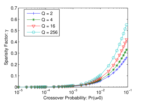
Figure 2: Lower bound of $\gamma$ to achieve the optimum compression ratio for $N\rightarrow\infty$, according to (66)

Figure 3: Optimum asymptotic achievable compression ratio in function of $\mathcal{H}\left(\mathsf{\mathsf{\Theta}}\right)/\log Q$, according to (67), for a crossover probability equal to $0.01$, $0.05$, $0.1$, and $0.2$ respectively, and without noise

V Sufficient Condition in Presence of Sensing Noise

This section performs an achievability study in presence of sensing noise by considering the conditional pmf $p_{\mathsf{x}\mid\Theta}$. The communication noise $\mathbf{u}^{M}$ is first neglected to simplify the problem (NS case). The extension to the NCS case is easily obtained from the NS case. Assume that $\boldsymbol{\theta}^{N}$ is the true state vector and that $\mathbf{x}^{N}$ represents the measurements of the sensors. The sink receives $\mathbf{y}^{M}=\mathbf{A}\mathbf{x}^{N}$. The a posteriori pmf (7) can be written as

$$p\left(\boldsymbol{\theta}^{N}\mid\mathbf{y}^{M},\mathbf{A}\right)\propto\sum_{\mathbf{z}^{N}\in\mathbb{F}_{Q}^{N}}p\left(\boldsymbol{\theta}^{N}\right)p\left(\mathbf{z}^{N}\mid\boldsymbol{\theta}^{N}\right)1_{\mathbf{y}^{M}=\mathbf{A}\mathbf{z}^{N}}.$$ (83)

In the case of MAP estimation, an error occurs if there exists a vector $\mathbf{\boldsymbol{\varphi}}^{N}\in\mathbb{F}_{Q}^{N}\setminus\left\{\boldsymbol{\theta}^{N}\right\}$ such that

$$\sum_{\mathbf{z}^{N}\in\mathbb{F}_{Q}^{N}}p\left(\boldsymbol{\theta}^{N},\mathbf{z}^{N}\right)1_{\mathbf{y}^{M}=\mathbf{A}\mathbf{z}^{N}}\leq\sum_{\mathbf{z}^{N}\in\mathbb{F}_{Q}^{N}}p\left(\mathbf{\boldsymbol{\varphi}}^{N},\mathbf{z}^{N}\right)1_{\mathbf{y}^{M}=\mathbf{A}\mathbf{z}^{N}}.$$ (84)

$\boldsymbol{\theta}^{N}$ and $\mathbf{x}^{N}$ are considered as fixed, but unknown. The decoder has knowledge of $\mathbf{A}$ and $\mathbf{y}^{M}=\mathbf{A}\mathbf{x}^{N}$, thus an alternative way to express (84) is

$$\sum_{\mathbf{z}^{N}\in\mathbb{F}_{Q}^{N}}p\left(\boldsymbol{\theta}^{N},\mathbf{z}^{N}\right)1_{\mathbf{A}\mathbf{x}^{N}=\mathbf{A}\mathbf{z}^{N}}\leq\sum_{\mathbf{z}^{N}\in\mathbb{F}_{Q}^{N}}p\left(\mathbf{\boldsymbol{\varphi}}^{N},\mathbf{z}^{N}\right)1_{\mathbf{A}\mathbf{x}^{N}=\mathbf{A}\mathbf{z}^{N}}.$$ (85)

V-A Achievability Study

We begin with the extension of the basic weakly typical set as introduced in Section IV-A. For any $\varepsilon>0$ and $N\in\mathbb{N}^{+}$, based on $\mathcal{A}_{\left[\mathsf{\Theta}\right]\varepsilon}^{N}$ for $\boldsymbol{\theta}^{N}$, one defines the weakly conditional typical set $\mathcal{A}_{\left[\mathsf{x}\mid\mathsf{\Theta}\right]\varepsilon}^{N}\left(\boldsymbol{\theta}^{N}\right)$ for $\mathbf{x}^{N}$, which is conditionally distributed with respect to $p_{\mathsf{x}\mid\mathsf{\Theta}}$, with $\boldsymbol{\theta}^{N}\in\mathcal{A}_{\left[\mathsf{\Theta}\right]\varepsilon}^{N}$,

$$\mathcal{A}_{\left[\mathsf{x}\mid\mathsf{\Theta}\right]\varepsilon}^{N}\left(\boldsymbol{\theta}^{N}\right)=\left\{\mathbf{x}^{N}\in\mathbb{F}_{Q}^{N}\mbox{ such that }\left|-\frac{1}{N}\log p\left(\mathbf{x}^{N}\mid\boldsymbol{\theta}^{N}\right)-\mathcal{H}\left(\mathsf{x}\mid\mathsf{\Theta}\right)\right|\leq\varepsilon\right\}.$$ (86)

Since $\mathcal{H}\left(\mathsf{\mathsf{\Theta}},\mathsf{x}\right)=\mathcal{H}\left(\mathsf{\mathsf{\Theta}}\right)+\mathcal{H}\left(\mathsf{x}\mid\mathsf{\Theta}\right)$, if $\boldsymbol{\theta}^{N}\in\mathcal{A}_{\left[\mathsf{\Theta}\right]\varepsilon}^{N}$ and $\mathbf{x}^{N}\in\mathcal{A}_{\left[\mathsf{x}\mid\mathsf{\Theta}\right]\varepsilon}^{N}\left(\boldsymbol{\theta}^{N}\right)$, then $\left(\boldsymbol{\theta}^{N},\mathbf{x}^{N}\right)\in\mathcal{A}_{\left[\mathsf{\Theta},\mathsf{x}\right]2\varepsilon}^{N}$ by consistency, where $\mathcal{A}_{\left[\mathsf{\Theta},\mathsf{x}\right]2\varepsilon}^{N}$ denotes the weakly joint typical set, i.e., the set of pairs $\left(\boldsymbol{\theta}^{N},\mathbf{x}^{N}\right)\in\mathbb{F}_{Q}^{N}\times\mathbb{F}_{Q}^{N}$ such that

$$\left|-\frac{1}{N}\log p\left(\boldsymbol{\theta}^{N},\mathbf{x}^{N}\right)-\mathcal{H}\left(\mathsf{\mathsf{\Theta}},\mathsf{x}\right)\right|\leq 2\varepsilon.$$ (87)

For any $\varepsilon>0$ there exist an $N_{\varepsilon}$ such that for all $N\geq N_{\varepsilon}$ and for any $\boldsymbol{\theta}^{N}\in\mathcal{A}_{\left[\mathsf{\Theta}\right]\varepsilon}^{N}$, one has $\Pr\left\{\boldsymbol{\mathsf{x}}^{N}\in\mathcal{A}_{\left[\mathsf{x}\mid\mathsf{\Theta}\right]\varepsilon}^{N}\left(\boldsymbol{\theta}^{N}\right)\right\}\geq 1-\varepsilon$ and $\Pr\left\{\left(\boldsymbol{\mathsf{\Theta}}^{N},\boldsymbol{\mathsf{x}}^{N}\right)\in\mathcal{A}_{\left[\mathsf{\Theta},\mathsf{x}\right]2\varepsilon}^{N}\right\}\geq 1-2\varepsilon$. The cardinality of the set $\mathcal{A}_{\left[\mathsf{\Theta},\mathsf{x}\right]2\varepsilon}^{N}$ satisfies

$$\left|\mathcal{A}_{\left[\mathsf{\Theta},\mathsf{x}\right]2\varepsilon}^{N}\right|\leq 2^{N\left(\mathcal{H}\left(\mathsf{\mathsf{\Theta}},\mathsf{x}\right)+2\varepsilon\right)}.$$ (88)

One may have $\varepsilon$ arbitrary close to zero as $N\rightarrow\infty$.

Considering $\mathcal{A}_{\left[\mathsf{\Theta},\mathsf{x}\right]2\varepsilon}^{N}$, the estimation error probability is bounded by

$$P_{\textrm{e}} \leq \sum_{\left(\boldsymbol{\theta}^{N},\mathbf{x}^{N}\right)\in\mathcal{A}_{\left[\mathsf{\Theta},\mathsf{x}\right]2\varepsilon}^{N}}p\left(\boldsymbol{\theta}^{N},\mathbf{x}^{N}\right)\Pr\left\{\textrm{error}\mid\boldsymbol{\theta}^{N},\mathbf{x}^{N}\right\}+\sum_{\left(\boldsymbol{\theta}^{N},\mathbf{x}^{N}\right)\notin\mathcal{A}_{\left[\mathsf{\Theta},\mathsf{x}\right]2\varepsilon}^{N}}p\left(\boldsymbol{\theta}^{N},\mathbf{x}^{N}\right)$$ (89)

$$\leq \sum_{\left(\boldsymbol{\theta}^{N},\mathbf{x}^{N}\right)\in\mathcal{A}_{\left[\mathsf{\Theta},\mathsf{x}\right]2\varepsilon}^{N}}p\left(\boldsymbol{\theta}^{N},\mathbf{x}^{N}\right)\cdot\Pr\left\{\textrm{error}\mid\boldsymbol{\theta}^{N},\mathbf{x}^{N}\right\}+2\varepsilon,$$

Errors appear mainly due to a bad sensing matrix. Averaging over all $\mathbf{A}\in\mathbb{F}_{Q}^{M\times N}$, (89) becomes

$$P_{\textrm{e}}\leq\sum_{\mathbf{A}\in\mathbb{F}_{Q}^{M\times N}}p\left(\mathbf{A}\right)\sum_{\boldsymbol{\theta}^{N}\in\mathcal{A}_{\left[\mathsf{\Theta}\right]\varepsilon}^{N}}\sum_{\mathbf{x}^{N}\in\mathcal{A}_{\left[\mathsf{x}\mid\mathsf{\Theta}\right]\varepsilon}^{N}\left(\boldsymbol{\theta}^{N}\right)}p\left(\boldsymbol{\theta}^{N},\mathbf{x}^{N}\right)\Pr\left\{\textrm{error}\mid\boldsymbol{\theta}^{N},\mathbf{x}^{N},\mathbf{A}\right\}+2\varepsilon,$$ (90)

where $p\left(\mathbf{A}\right)=\Pr\left\{\boldsymbol{\mathsf{A}}=\mathbf{A}\right\}$. $\Pr\left\{\textrm{error}\mid\boldsymbol{\theta}^{N},\mathbf{x}^{N},\mathbf{A}\right\}$ can be written as

$$\Pr\left\{\textrm{error}\mid\boldsymbol{\theta}^{N},\mathbf{x}^{N},\mathbf{A}\right\}=\begin{cases}1&\mbox{ if }\exists\,\mathbf{\boldsymbol{\varphi}}^{N}\in\mathbb{F}_{Q}^{N}\setminus\left\{\boldsymbol{\theta}^{N}\right\}\textrm{ s.t. \eqref{eq:conditionNS2} holds,}\\ 0&\mbox{ if }\forall\,\mathbf{\boldsymbol{\varphi}}^{N}\in\mathbb{F}_{Q}^{N}\setminus\left\{\boldsymbol{\theta}^{N}\right\},\textrm{ \eqref{eq:conditionNS2} does not hold.}\end{cases}$$ (91)

Using again the idea of Lemma 1, the conditional error probability is bounded by

$$\Pr\left\{\textrm{error}\mid\boldsymbol{\theta}^{N},\mathbf{x}^{N},\mathbf{A}\right\}\leq\sum_{\mathbf{\boldsymbol{\varphi}}^{N}\in\mathbb{F}_{Q}^{N}\setminus\left\{\boldsymbol{\theta}^{N}\right\}}\frac{\sum_{\mathbf{z}_{1}^{N}\in\mathbb{F}_{Q}^{N}}p\left(\mathbf{\boldsymbol{\varphi}}^{N},\mathbf{z}_{1}^{N}\right)1_{\mathbf{A}\mathbf{x}^{N}=\mathbf{A}\mathbf{z}_{1}^{N}}}{\sum_{\mathbf{z}_{2}^{N}\in\mathbb{F}_{Q}^{N}}p\left(\boldsymbol{\theta}^{N},\mathbf{z}_{2}^{N}\right)1_{\mathbf{A}\mathbf{x}^{N}=\mathbf{A}\mathbf{z}_{2}^{N}}}.$$ (92)

From (90) and (92), one gets

$$P_{\textrm{e}}\leq\sum_{{}_{\boldsymbol{\theta}^{N}\in\mathcal{A}_{\left[\mathsf{\Theta}\right]\varepsilon}^{N}}^{\mathbf{A}\in\mathbb{F}_{Q}^{M\times N}}}p\left(\mathbf{A}\right)\sum_{\mathbf{x}^{N}\in\mathcal{A}_{\left[\mathsf{x}\mid\mathsf{\Theta}\right]\varepsilon}^{N}\left(\boldsymbol{\theta}^{N}\right)}p\left(\boldsymbol{\theta}^{N},\mathbf{x}^{N}\right)\sum_{\mathbf{\boldsymbol{\varphi}}^{N}\in\mathbb{F}_{Q}^{N}\setminus\left\{\boldsymbol{\theta}^{N}\right\}}\frac{\sum_{\mathbf{z}_{1}^{N}\in\mathbb{F}_{Q}^{N}}p\left(\mathbf{\boldsymbol{\varphi}}^{N},\mathbf{z}_{1}^{N}\right)1_{\mathbf{A}\mathbf{x}^{N}=\mathbf{A}\mathbf{z}_{1}^{N}}}{\sum_{\mathbf{z}_{2}^{N}\in\mathbb{F}_{Q}^{N}}p\left(\boldsymbol{\theta}^{N},\mathbf{z}_{2}^{N}\right)1_{\mathbf{A}\mathbf{x}^{N}=\mathbf{A}\mathbf{z}_{2}^{N}}}+2\varepsilon.$$ (93)

Now, for some $\boldsymbol{\theta}^{N}\in\mathcal{A}_{\left[\mathsf{\Theta}\right]\varepsilon}^{N}$, consider the direct image by $\mathbf{A}$ of the conditional typical set $\mathcal{A}_{\left[\mathsf{x}\mid\mathsf{\Theta}\right]\varepsilon}^{N}\left(\boldsymbol{\theta}^{N}\right)$

$$\mathcal{Y}_{\varepsilon}\left(\mathbf{A},\boldsymbol{\theta}^{N}\right)=\left\{\mathbf{y}^{M}=\mathbf{A}\mathbf{x}^{N},\textrm{ for all }\;\mathbf{x}^{N}\in\mathcal{A}_{\left[\mathsf{x}\mid\mathsf{\Theta}\right]\varepsilon}^{N}\left(\boldsymbol{\theta}^{N}\right)\right\}.$$ (94)

Lemma 3. For any arbitrary real-valued function $h\left(\mathbf{x}^{N}\right)$ with $\mathbf{x}^{N}\in\mathbb{F}_{Q}^{N}$, one has

$$\sum_{\mathbf{x}^{N}\in\mathcal{A}_{\left[\mathsf{x}\mid\mathsf{\Theta}\right]\varepsilon}^{N}\left(\boldsymbol{\theta}^{N}\right)}h\left(\mathbf{x}^{N}\right)=\sum_{\mathbf{y}^{M}\in\mathcal{Y}_{\varepsilon}\left(\mathbf{A},\boldsymbol{\theta}^{N}\right)}\sum_{\mathbf{x}^{N}\in\mathcal{A}_{\left[\mathsf{x}\mid\mathsf{\Theta}\right]\varepsilon}^{N}\left(\boldsymbol{\theta}^{N}\right)}h\left(\mathbf{x}^{N}\right)1_{\mathbf{y}^{M}=\mathbf{A}\mathbf{x}^{N}}.$$ (95)

Proof.

For a given $\mathbf{y}^{M}\in\mathcal{Y}_{\varepsilon}\left(\mathbf{A},\boldsymbol{\theta}^{N}\right)$, consider the set

$$\mathcal{X}_{\varepsilon}\left(\mathbf{y}^{M},\mathbf{A},\boldsymbol{\theta}^{N}\right)=\left\{\mathbf{x}^{N}\in\mathcal{A}_{\left[\mathsf{x}\mid\mathsf{\Theta}\right]\varepsilon}^{N}\left(\boldsymbol{\theta}^{N}\right)\mbox{ such that }\mathbf{y}^{M}=\mathbf{A}\mathbf{x}^{N}\right\}.$$ (96)

Then one has

$$\mathcal{A}_{\left[\mathsf{x}\mid\mathsf{\Theta}\right]\varepsilon}^{N}\left(\boldsymbol{\theta}^{N}\right)=\bigcup_{\mathbf{y}^{M}\in\mathcal{Y}_{\varepsilon}\left(\mathbf{A},\boldsymbol{\theta}^{N}\right)}\mathcal{X}_{\varepsilon}\left(\mathbf{y}^{M},\mathbf{A},\boldsymbol{\theta}^{N}\right),$$ (97)

with $\mathcal{X}_{\varepsilon}\left(\mathbf{y}_{i}^{M},\mathbf{A},\boldsymbol{\theta}^{N}\right)\cap\mathcal{X}_{\varepsilon}\left(\mathbf{y}_{j}^{M},\mathbf{A},\boldsymbol{\theta}^{N}\right)=\emptyset$ for any $\mathbf{y}_{i}^{M}\neq\mathbf{y}_{j}^{M},$ since the multiplication by $\mathbf{A}$ is a surjection from $\mathcal{A}_{\left[\mathsf{x}\mid\mathsf{\Theta}\right]\varepsilon}^{N}\left(\boldsymbol{\theta}^{N}\right)$ to $\mathcal{Y}_{\varepsilon}\left(\mathbf{A},\boldsymbol{\theta}^{N}\right)$. So any sum over $\mathbf{x}^{N}\in\mathcal{A}_{\left[\mathsf{x}\mid\mathsf{\Theta}\right]\varepsilon}^{N}\left(\boldsymbol{\theta}^{N}\right)$ can be decomposed as

$$\sum_{\mathbf{x}^{N}\in\mathcal{A}_{\left[\mathsf{x}\mid\mathsf{\Theta}\right]\varepsilon}^{N}\left(\boldsymbol{\theta}^{N}\right)}h\left(\mathbf{x}^{N}\right) = \sum_{\mathbf{y}^{M}\in\mathcal{Y}_{\varepsilon}\left(\mathbf{A},\boldsymbol{\theta}^{N}\right)}\sum_{\mathbf{x}^{N}\in\mathcal{X}_{\varepsilon}\left(\mathbf{y}^{M},\mathbf{A},\boldsymbol{\theta}^{N}\right)}h\left(\mathbf{x}^{N}\right)$$ (98)

$$= \sum_{\mathbf{y}^{M}\in\mathcal{Y}_{\varepsilon}\left(\mathbf{A},\boldsymbol{\theta}^{N}\right)}\sum_{\mathbf{x}^{N}\in\mathcal{A}_{\left[\mathsf{x}\mid\mathsf{\Theta}\right]\varepsilon}^{N}\left(\boldsymbol{\theta}^{N}\right)}h\left(\mathbf{x}^{N}\right)1_{\mathbf{y}^{M}=\mathbf{A}\mathbf{x}^{N}}.$$

∎

Applying (95) to (93), one obtains

$$P_{\textrm{e}} \leq\sum_{{}_{\boldsymbol{\theta}^{N}\in\mathcal{A}_{\left[\mathsf{\Theta}\right]\varepsilon}^{N}}^{\mathbf{A}\in\mathbb{F}_{Q}^{M\times N}}}p\left(\mathbf{A}\right)\sum_{\mathbf{y}^{M}\in\mathcal{Y}_{\varepsilon}\left(\mathbf{A},\boldsymbol{\theta}^{N}\right)}\sum_{\mathbf{x}^{N}\in\mathcal{A}_{\left[\mathsf{x}\mid\mathsf{\Theta}\right]\varepsilon}^{N}\left(\boldsymbol{\theta}^{N}\right)}p\left(\boldsymbol{\theta}^{N},\mathbf{x}^{N}\right)1_{\mathbf{y}^{M}=\mathbf{A}\mathbf{x}^{N}}$$

$$\cdot\left(\sum_{\mathbf{\boldsymbol{\varphi}}^{N}\in\mathbb{F}_{Q}^{N}\setminus\left\{\boldsymbol{\theta}^{N}\right\}}\frac{\sum_{\mathbf{z}_{1}^{N}\in\mathbb{F}_{Q}^{N}}p\left(\mathbf{\boldsymbol{\varphi}}^{N},\mathbf{z}_{1}^{N}\right)1_{\mathbf{y}^{M}=\mathbf{A}\mathbf{z}_{1}^{N}}}{\sum_{\mathbf{z}_{2}^{N}\in\mathbb{F}_{Q}^{N}}p\left(\boldsymbol{\theta}^{N},\mathbf{z}_{2}^{N}\right)1_{\mathbf{y}^{M}=\mathbf{A}\mathbf{z}_{2}^{N}}}\right)+2\varepsilon$$

$$=\sum_{{}_{\boldsymbol{\theta}^{N}\in\mathcal{A}_{\left[\mathsf{\Theta}\right]\varepsilon}^{N}}^{\mathbf{A}\in\mathbb{F}_{Q}^{M\times N}}}p\left(\mathbf{A}\right)\sum_{\mathbf{y}^{M}\in\mathcal{Y}_{\varepsilon}\left(\mathbf{A},\boldsymbol{\theta}^{N}\right)}\left(\sum_{\mathbf{\boldsymbol{\varphi}}^{N}\in\mathbb{F}_{Q}^{N}\setminus\left\{\boldsymbol{\theta}^{N}\right\}}\sum_{\mathbf{z}_{1}^{N}\in\mathbb{F}_{Q}^{N}}p\left(\mathbf{\boldsymbol{\varphi}}^{N},\mathbf{z}_{1}^{N}\right)\cdot 1_{\mathbf{y}^{M}=\mathbf{A}\mathbf{z}_{1}^{N}}\right)$$

$$\cdot\left(\frac{\sum_{\mathbf{x}^{N}\in\mathcal{A}_{\left[\mathsf{x}\mid\mathsf{\Theta}\right]\varepsilon}^{N}\left(\boldsymbol{\theta}^{N}\right)}p\left(\boldsymbol{\theta}^{N},\mathbf{x}^{N}\right)1_{\mathbf{y}^{M}=\mathbf{A}\mathbf{x}^{N}}}{\sum_{\mathbf{z}_{2}^{N}\in\mathbb{F}_{Q}^{N}}p\left(\boldsymbol{\theta}^{N},\mathbf{z}_{2}^{N}\right)1_{\mathbf{y}^{M}=\mathbf{A}\mathbf{z}_{2}^{N}}}\right)+2\varepsilon$$

$$\leq\sum_{{}_{\boldsymbol{\theta}^{N}\in\mathcal{A}_{\left[\mathsf{\Theta}\right]\varepsilon}^{N}}^{\mathbf{A}\in\mathbb{F}_{Q}^{M\times N}}}p\left(\mathbf{A}\right)\sum_{\mathbf{y}^{M}\in\mathcal{Y}_{\varepsilon}\left(\mathbf{A},\boldsymbol{\theta}^{N}\right)}\left(\sum_{\mathbf{\boldsymbol{\varphi}}^{N}\in\mathbb{F}_{Q}^{N}\setminus\left\{\boldsymbol{\theta}^{N}\right\}}\sum_{\mathbf{z}_{1}^{N}\in\mathbb{F}_{Q}^{N}}p\left(\mathbf{\boldsymbol{\varphi}}^{N},\mathbf{z}_{1}^{N}\right)1_{\mathbf{y}^{M}=\mathbf{A}\mathbf{z}_{1}^{N}}\right)+2\varepsilon,$$ (99)

since we have

$$\frac{\sum_{\mathbf{x}^{N}\in\mathcal{A}_{\left[\mathsf{x}\mid\mathsf{\Theta}\right]\varepsilon}^{N}\left(\boldsymbol{\theta}^{N}\right)}p\left(\boldsymbol{\theta}^{N},\mathbf{x}^{N}\right)1_{\mathbf{y}^{M}=\mathbf{A}\mathbf{x}^{N}}}{\sum_{\mathbf{z}_{2}^{N}\in\mathbb{F}_{Q}^{N}}p\left(\boldsymbol{\theta}^{N},\mathbf{z}_{2}^{N}\right)1_{\mathbf{y}^{M}=\mathbf{A}\mathbf{z}_{2}^{N}}}\leq 1.$$ (100)

The bound (100) is tight because for $N$ sufficiently large, the probability of the non-typical set vanishes. Recall that $\mathbf{y}^{M}=\mathbf{A}\mathbf{x}^{N}$, even though $\mathbf{x}^{N}$ is not explicit in (99). As a vector $\mathbf{y}^{M}$ may correspond to several $\mathbf{x}^{N}$s, (99) is further bounded by

$$P_{\textrm{e}} \leq \sum_{{}_{\boldsymbol{\theta}^{N}\in\mathcal{A}_{\left[\mathsf{\Theta}\right]\varepsilon}^{N}}^{\mathbf{A}\in\mathbb{F}_{Q}^{M\times N}}}p\left(\mathbf{A}\right)\sum_{\mathbf{x}^{N}\in\mathcal{A}_{\left[\mathsf{x}\mid\mathsf{\Theta}\right]\varepsilon}^{N}\left(\boldsymbol{\theta}^{N}\right)}\sum_{{}_{\quad\mathbf{z}_{1}^{N}\in\mathbb{F}_{Q}^{N}}^{\mathbf{\boldsymbol{\varphi}}^{N}\in\mathbb{F}_{Q}^{N}\setminus\left\{\boldsymbol{\theta}^{N}\right\}}}p\left(\mathbf{\boldsymbol{\varphi}}^{N},\mathbf{z}_{1}^{N}\right)1_{\mathbf{A}\mathbf{x}^{N}=\mathbf{A}\mathbf{z}_{1}^{N}}+2\varepsilon$$ (101)

$$\leq \sum_{{}_{\mathbf{\boldsymbol{\varphi}}^{N}\in\mathbb{F}_{Q}^{N}\setminus\left\{\boldsymbol{\theta}^{N}\right\}}^{\;\;\;\;\boldsymbol{\theta}^{N}\in\mathcal{A}_{\left[\mathsf{\Theta}\right]\varepsilon}^{N}}}\sum_{{}_{\;\>\quad\mathbf{z}_{1}^{N}\in\mathbb{F}_{Q}^{N}}^{\mathbf{x}^{N}\in\mathcal{A}_{\left[\mathsf{x}\mid\mathsf{\Theta}\right]\varepsilon}^{N}\left(\boldsymbol{\theta}^{N}\right)}}p\left(\mathbf{\boldsymbol{\varphi}}^{N},\mathbf{z}_{1}^{N}\right)\sum_{\mathbf{A}\in\mathbb{F}_{Q}^{M\times N}}p\left(\mathbf{A}\right)1_{\mathbf{A}\mathbf{x}^{N}=\mathbf{A}\mathbf{z}_{1}^{N}}+2\varepsilon.$$

Since

$$\sum_{\mathbf{A}\in\mathbb{F}_{Q}^{M\times N}}p\left(\mathbf{A}\right)1_{\mathbf{A}\mathbf{x}^{N}=\mathbf{A}\mathbf{z}_{1}^{N}}=\Pr\left\{\boldsymbol{\mathsf{A}}\mathbf{x}^{N}=\boldsymbol{\mathsf{A}}\mathbf{z}_{1}^{N}\right\},$$ (102)

one gets

$$P_{\textrm{e}}\leq\sum_{{}_{\mathbf{\boldsymbol{\varphi}}^{N}\in\mathbb{F}_{Q}^{N}\setminus\left\{\boldsymbol{\theta}^{N}\right\}}^{\;\;\;\;\boldsymbol{\theta}^{N}\in\mathcal{A}_{\left[\mathsf{\Theta}\right]\varepsilon}^{N}}}\sum_{{}_{\;\>\quad\mathbf{z}_{1}^{N}\in\mathbb{F}_{Q}^{N}}^{\mathbf{x}^{N}\in\mathcal{A}_{\left[\mathsf{x}\mid\mathsf{\Theta}\right]\varepsilon}^{N}\left(\boldsymbol{\theta}^{N}\right)}}p\left(\mathbf{\boldsymbol{\varphi}}^{N},\mathbf{z}_{1}^{N}\right)\Pr\left\{\boldsymbol{\mathsf{A}}\mathbf{x}^{N}=\boldsymbol{\mathsf{A}}\mathbf{z}_{1}^{N}\right\}+2\varepsilon.$$ (103)

Suppose that $\left\|\mathbf{x}^{N}-\mathbf{z}_{1}^{N}\right\|_{0}=d$. If $d=0$, $\Pr\left\{\boldsymbol{\mathsf{A}}\mathbf{x}^{N}=\boldsymbol{\mathsf{A}}\mathbf{z}_{1}^{N}\right\}$ equals 1. Otherwise we can apply Lemma 2, without communication noise, $\Pr\left\{\boldsymbol{\mathsf{A}}\mathbf{x}^{N}=\boldsymbol{\mathsf{A}}\mathbf{z}_{1}^{N}\right\}=f\left(d,0;\gamma,Q,M\right)$ . Depending on $d$ being zero or not, $P_{\mathcal{A}}$ is split as follows

$$P_{\textrm{e}}\leq P_{\mathcal{A}_{1}}+P_{\mathcal{A}_{2}}+2\varepsilon,$$ (104)

where

$$P_{\mathcal{A}_{1}}=\sum_{{}_{\mathbf{\boldsymbol{\varphi}}^{N}\in\mathbb{F}_{Q}^{N}\setminus\left\{\boldsymbol{\theta}^{N}\right\}}^{\;\;\;\;\boldsymbol{\theta}^{N}\in\mathcal{A}_{\left[\mathsf{\Theta}\right]\varepsilon}^{N}}}\sum_{\mathbf{z}_{1}^{N}\in\mathcal{A}_{\left[\mathsf{x}\mid\mathsf{\Theta}\right]\varepsilon}^{N}\left(\boldsymbol{\theta}^{N}\right)}p\left(\mathbf{\boldsymbol{\varphi}}^{N},\mathbf{z}_{1}^{N}\right),$$ (105)

and

$$P_{\mathcal{A}_{2}}=\sum_{{}_{\mathbf{\boldsymbol{\varphi}}^{N}\in\mathbb{F}_{Q}^{N}\setminus\left\{\boldsymbol{\theta}^{N}\right\}}^{\;\;\;\;\boldsymbol{\theta}^{N}\in\mathcal{A}_{\left[\mathsf{\Theta}\right]\varepsilon}^{N}}}\sum_{{}_{\>\>\>\mathbf{z}_{1}^{N}\in\mathbb{F}_{Q}^{N}\setminus\left\{\mathbf{x}^{N}\right\}}^{\mathbf{x}^{N}\in\mathcal{A}_{\left[\mathsf{x}\mid\mathsf{\Theta}\right]\varepsilon}^{N}\left(\boldsymbol{\theta}^{N}\right)}}p\left(\mathbf{\boldsymbol{\varphi}}^{N},\mathbf{z}_{1}^{N}\right)\Pr\left\{\boldsymbol{\mathsf{A}}\mathbf{x}^{N}=\boldsymbol{\mathsf{A}}\mathbf{z}_{1}^{N}\right\}.$$ (106)

Lemma 4. A sufficient condition for $P_{\mathcal{A}_{1}}\leq 2\varepsilon$ is that, for any pair of vectors $(\boldsymbol{\theta}^{N},\mathbf{\boldsymbol{\varphi}}^{N})\in\mathcal{A}_{\left[\mathsf{\Theta}\right]\varepsilon}^{N}\times\mathcal{A}_{\left[\mathsf{\Theta}\right]\varepsilon}^{N}$ such that $\boldsymbol{\theta}^{N}\neq\mathbf{\boldsymbol{\varphi}}^{N}$,

$$\mathcal{A}_{\left[\mathsf{x}\mid\mathsf{\Theta}\right]\varepsilon}^{N}\left(\boldsymbol{\theta}^{N}\right)\cap\mathcal{A}_{\left[\mathsf{x}\mid\mathsf{\Theta}\right]\varepsilon}^{N}\left(\mathbf{\boldsymbol{\varphi}}^{N}\right)=\emptyset.$$ (107)

Proof.

Assume that (107) is satisfied. Changing the order of summation, (105) becomes

$$P_{\mathcal{A}_{1}}=\sum_{\mathbf{\boldsymbol{\varphi}}^{N}\in\mathbb{F}_{Q}^{N}}p\left(\mathbf{\boldsymbol{\varphi}}^{N}\right)\sum_{{}_{\,\mathbf{z}_{1}^{N}\in\mathcal{A}_{\left[\mathsf{x}\mid\mathsf{\Theta}\right]\varepsilon}^{N}\left(\boldsymbol{\theta}^{N}\right)}^{\boldsymbol{\theta}^{N}\in\mathcal{A}_{\left[\mathsf{\Theta}\right]\varepsilon}^{N}\setminus\left\{\mathbf{\boldsymbol{\varphi}}^{N}\right\}}}p\left(\mathbf{z}_{1}^{N}\mid\mathbf{\boldsymbol{\varphi}}^{N}\right),$$ (108)

which can be further decomposed as $P_{\mathcal{A}_{1}}=P_{\mathcal{A}_{11}}+P_{\mathcal{A}_{12}}$, with

$$P_{\mathcal{A}_{11}} = \sum_{\mathbf{\boldsymbol{\varphi}}^{N}\in\mathcal{A}_{\left[\mathsf{\Theta}\right]\varepsilon}^{N}}p\left(\mathbf{\boldsymbol{\varphi}}^{N}\right)\sum_{{}_{\,\mathbf{z}_{1}^{N}\in\mathcal{A}_{\left[\mathsf{x}\mid\mathsf{\Theta}\right]\varepsilon}^{N}\left(\boldsymbol{\theta}^{N}\right)}^{\boldsymbol{\theta}^{N}\in\mathcal{A}_{\left[\mathsf{\Theta}\right]\varepsilon}^{N}\setminus\left\{\mathbf{\boldsymbol{\varphi}}^{N}\right\}}}p\left(\mathbf{z}_{1}^{N}\mid\mathbf{\boldsymbol{\varphi}}^{N}\right)$$ (109)

$$\overset{(a)}{\leq} \sum_{\mathbf{\boldsymbol{\varphi}}^{N}\in\mathcal{A}_{\left[\mathsf{\Theta}\right]\varepsilon}^{N}}p\left(\mathbf{\boldsymbol{\varphi}}^{N}\right)\sum_{\mathbf{z}_{1}^{N}\in\mathbb{F}_{Q}^{N}\setminus\mathcal{A}_{\left[\mathsf{x}\mid\mathsf{\Theta}\right]\varepsilon}^{N}\left(\mathbf{\boldsymbol{\varphi}}^{N}\right)}p\left(\mathbf{z}_{1}^{N}\mid\mathbf{\boldsymbol{\varphi}}^{N}\right)$$

$$\leq \sum_{\mathbf{\boldsymbol{\varphi}}^{N}\in\mathcal{A}_{\left[\mathsf{\Theta}\right]\varepsilon}^{N}}p\left(\mathbf{\boldsymbol{\varphi}}^{N}\right)\varepsilon\leq\varepsilon,$$

where $(a)$ comes from the fact that if (107) is satisfied, one has

$$\bigcup_{\boldsymbol{\theta}^{N}\in\mathcal{A}_{\left[\mathsf{\Theta}\right]\varepsilon}^{N}\setminus\left\{\mathbf{\boldsymbol{\varphi}}^{N}\right\}}\mathcal{A}_{\left[\mathsf{x}\mid\mathsf{\Theta}\right]\varepsilon}^{N}\left(\boldsymbol{\theta}^{N}\right)\subseteq\mathbb{F}_{Q}^{N}\setminus\mathcal{A}_{\left[\mathsf{x}\mid\mathsf{\Theta}\right]\varepsilon}^{N}\left(\mathbf{\boldsymbol{\varphi}}^{N}\right).$$ (110)

On the other hand,

$$P_{\mathcal{A}_{12}} = \sum_{\mathbf{\boldsymbol{\varphi}}^{N}\in\mathbb{F}_{Q}^{N}\setminus\mathcal{A}_{\left[\mathsf{\Theta}\right]\varepsilon}^{N}}p\left(\mathbf{\boldsymbol{\varphi}}^{N}\right)\sum_{{}_{\mathbf{z}_{1}^{N}\in\mathcal{A}_{\left[\mathsf{x}\mid\mathsf{\Theta}\right]\varepsilon}^{N}\left(\boldsymbol{\theta}^{N}\right)}^{\quad\>\boldsymbol{\theta}^{N}\in\mathcal{A}_{\left[\mathsf{\Theta}\right]\varepsilon}^{N}}}p\left(\mathbf{z}_{1}^{N}\mid\mathbf{\boldsymbol{\varphi}}^{N}\right)$$ (111)

$$\leq \sum_{\mathbf{\boldsymbol{\varphi}}^{N}\in\mathbb{F}_{Q}^{N}\setminus\mathcal{A}_{\left[\mathsf{\Theta}\right]\varepsilon}^{N}}p\left(\mathbf{\boldsymbol{\varphi}}^{N}\right)\leq\varepsilon,$$

since for this part

$$\bigcup_{\boldsymbol{\theta}^{N}\in\mathcal{A}_{\left[\mathsf{\Theta}\right]\varepsilon}^{N}}\mathcal{A}_{\left[\mathsf{x}\mid\mathsf{\Theta}\right]\varepsilon}^{N}\left(\boldsymbol{\theta}^{N}\right)\subseteq\mathbb{F}_{Q}^{N}.$$ (112)

From (109) and (111), Lemma 4 is proved. ∎

Now consider the term (106),

$$P_{\mathcal{A}_{2}} = \sum_{d=1}^{N}\sum_{{}_{\mathbf{\boldsymbol{\varphi}}^{N}\in\mathbb{F}_{Q}^{N}\setminus\left\{\boldsymbol{\theta}^{N}\right\}}^{\;\;\;\;\boldsymbol{\theta}^{N}\in\mathcal{A}_{\left[\mathsf{\Theta}\right]\varepsilon}^{N}}}\sum_{{}_{\mathbf{z}_{1}^{N}\in\mathbb{F}_{Q}^{N}:\left\|\mathbf{x}^{N}-\mathbf{z}_{1}^{N}\right\|_{0}=d}^{\leavevmode\nobreak\ \leavevmode\nobreak\ \leavevmode\nobreak\ \mathbf{x}^{N}\in\mathcal{A}_{\left[\mathsf{x}\mid\mathsf{\Theta}\right]\varepsilon}^{N}\left(\boldsymbol{\theta}^{N}\right)}}p\left(\mathbf{\boldsymbol{\varphi}}^{N},\mathbf{z}_{1}^{N}\right)\cdot f\left(d,0;\gamma,Q,M\right)$$ (113)

$$\leq \sum_{d=1}^{\left\lfloor\beta N\right\rfloor}\sum_{{}_{\mathbf{\boldsymbol{\varphi}}^{N}\in\mathbb{F}_{Q}^{N}\setminus\left\{\boldsymbol{\theta}^{N}\right\}}^{\;\;\;\;\boldsymbol{\theta}^{N}\in\mathcal{A}_{\left[\mathsf{\Theta}\right]\varepsilon}^{N}}}\sum_{\mathbf{z}_{1}^{N}\in\mathbb{F}_{Q}^{N}}\sum_{\mathbf{x}^{N}\in\mathbb{F}_{Q}^{N}:\left\|\mathbf{x}^{N}-\mathbf{z}_{1}^{N}\right\|_{0}=d}p\left(\mathbf{\boldsymbol{\varphi}}^{N},\mathbf{z}_{1}^{N}\right)\cdot f\left(1,0;\gamma,Q,M\right)$$

$$+\sum_{{}_{\mathbf{x}^{N}\in\mathcal{A}_{\left[\mathsf{x}\mid\mathsf{\Theta}\right]\varepsilon}^{N}\left(\boldsymbol{\theta}^{N}\right)}^{\quad\boldsymbol{\theta}^{N}\in\mathcal{A}_{\left[\mathsf{\Theta}\right]\varepsilon}^{N}}}\sum_{{}_{\;\>\quad\,\mathbf{z}_{1}^{N}\in\mathbb{F}_{Q}^{N}}^{\mathbf{\boldsymbol{\varphi}}^{N}\in\mathcal{A}_{\left[\mathsf{\Theta}\right]\varepsilon}^{N}\setminus\left\{\boldsymbol{\theta}^{N}\right\}}}p\left(\mathbf{\boldsymbol{\varphi}}^{N},\mathbf{z}_{1}^{N}\right)\cdot f\left(\left\lceil\beta N\right\rceil,0;\gamma,Q,M\right),$$

which is similar to (59) in Section IV-A. For $N$ sufficient large, the condition on $M/N$ to ensure $P_{\mathcal{A}_{2}}$ tends to zero as $N\rightarrow\infty$ is

$$\frac{M}{N}>\frac{\mathcal{H}\left(\mathsf{\Theta},\mathsf{x}\right)+\varepsilon}{\log Q-\xi},$$ (114)

for some $\xi\in\mathbb{R}^{+}$. Finally, we have Proposition 4 to conclude the sufficient condition for reliable recovery in the NS case.

Proposition 4 (Sufficient condition, NS case).

In the NS case, fix an arbitrary small positive real number $\delta$, there exists $\varepsilon\in\mathbb{R}^{+}$, $\xi\in\mathbb{R}^{+}$, $N_{\delta}\in\mathbb{N}^{+}$ and $M_{\varepsilon}\in\mathbb{N}^{+}$ such that for any $N>N_{\delta}$ and $M>M_{\varepsilon}$, one has $P_{\textrm{e}}<\delta$ under MAP decoding if (107) and (114) hold. One can make both $\varepsilon$ and $\xi$ arbitrary close to $0$ as $N\rightarrow\infty$.

Finally, the NCS case, accounting for both communication and sensing noise, has to be considered.

Proposition 5 (Sufficient condition, NCS case).

Considering both communication noise and sensing noise, for $N$ and $M$ sufficient large and positive $\varepsilon$, $\xi$ arbitrary small, the reliable recovery can be ensured under MAP decoding if

• the communication noise is not uniformly distributed, (65)

• there is no overlapping between any two different weakly conditional typical sets, i.e., $\mathcal{A}_{\left[\mathsf{x}\mid\mathsf{\Theta}\right]\varepsilon}^{N}\left(\boldsymbol{\theta}^{N}\right)\cap\mathcal{A}_{\left[\mathsf{x}\mid\mathsf{\Theta}\right]\varepsilon}^{N}\left(\mathbf{\boldsymbol{\varphi}}^{N}\right)=\emptyset$ for any two typical but different $\boldsymbol{\theta}^{N}$ and $\mathbf{\boldsymbol{\varphi}}^{N}$,

• the sparsity factor satisfies the constraint in (66),

• the compression ratio $M/N$ is lower bounded by

  $$\frac{M}{N}>\frac{\mathcal{H}\left(\mathsf{\Theta},\mathsf{x}\right)+\varepsilon}{\log Q-H\left(p_{\mathsf{u}}\right)-\xi},$$ (115)

The derivations are similar to those of Proposition 3 and Proposition 4.

V-B Discussion and Numerical Results

When comparing the necessary condition in Proposition 1 and the sufficient condition in Proposition 5, an interesting fact is that $\mathcal{H}\left(\mathsf{\Theta}\mid\mathsf{x}\right)=0$ is a sufficient condition to have (107). This implies that the value of $\boldsymbol{\theta}^{N}$ should be fixed almost surely, as long as $\mathbf{x}^{N}$ is known. So, (107) is helpful to interpret (12), justifying the need for the conditional entropy $\mathcal{H}\left(\mathsf{\Theta}\mid\mathsf{x}\right)$ to tend to zero as $N$ increases. This condition may be satisfied since $\left|\mathcal{A}_{\left[\mathsf{\Theta}\right]\varepsilon}^{N}\right|\ll\left|\mathbb{F}_{Q}^{N}\right|$ as long as $\mathcal{H}\left(\mathsf{\Theta}\right)<\log Q$. The entropy rate $\mathcal{H}\left(\mathsf{\Theta}\right)$ can be very small, Appendix B presents a possible situation where $\mathcal{H}\left(\mathsf{\Theta}\right)=0$. Another implicit constraint resulting from (107) is

$$\sum_{\boldsymbol{\theta}^{N}\in\mathcal{A}_{\left[\mathsf{\Theta}\right]\varepsilon}^{N}}\mathcal{A}_{\left[\mathsf{x}\mid\mathsf{\Theta}\right]\varepsilon}^{N}\left(\boldsymbol{\theta}^{N}\right)\leq\left|\mathbb{F}_{Q}^{N}\right|$$ (116)

which means that

$$\mathcal{H}\left(\mathsf{\Theta},\mathsf{x}\right)\leq\log Q.$$ (117)

Consider a communication noise with $\Pr\left(\mathsf{u}\neq 0\right)=0.1$ and the transition pmf

$$p(x_{n}\mid\theta_{n})=\begin{cases}1-\Pr\left(\mathsf{x}\neq\mathsf{\Theta}\right)&\textrm{if }x_{n}=\theta_{n}\\ \frac{\Pr\left(\mathsf{x}\neq\mathsf{\Theta}\right)}{Q-1}&\textrm{if }x_{n}\in\mathbb{F}_{Q}^{N}\setminus\left\{\theta_{n}\right\}\end{cases},$$ (118)

where $\Pr\left(\mathsf{x}\neq\mathsf{\Theta}\right)$ denotes the probability of the sensing error. In Figure 4, the lower bound of $M/N$ is represented as a function of $\mathcal{H}\left(\mathsf{\mathsf{\Theta}}\right)/\log Q$, for different values of $Q$ and for different values of $\Pr\left(\mathsf{x}\neq\mathsf{\Theta}\right)$.

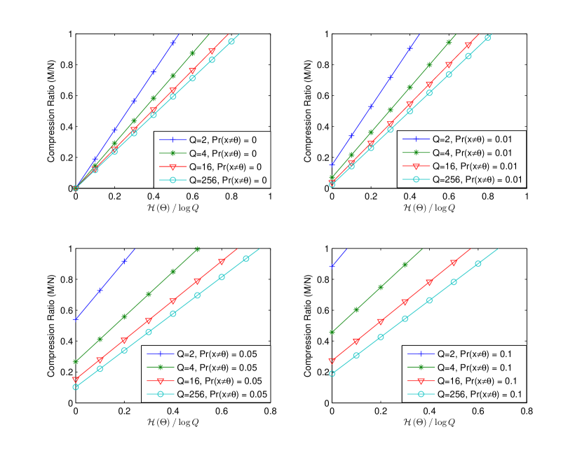
Figure 4: Optimum achievable compression ratio in function of $\mathcal{H}\left(\mathsf{\mathsf{\Theta}}\right)/\log Q$, according to (115), for the cases that $\Pr\left(\mathsf{x}\neq\mathsf{\Theta}\right)$ being $0$ (NC case), $0.01$, $0.05$, and $0.1$, respectively, when $\Pr\left(\mathsf{u}\neq 0\right)=0.1$

VI Conclusions and future work

In this paper we have considered robust Bayesian compressed sensing over finite fields under MAP decoding. Both asymptotically necessary and sufficient conditions of the compression ratio for reliable recovery are obtained and their convergence is also shown, even in the case of sparse sensing matrices. Several previous results have been generalized by considering a stationary and ergodic source model. Both communication noise and sensing noise have been taken into account. We have shown that the choice of the sparsity factor of the sensing matrix only depends on the communication noise. Since necessary and sufficient conditions asymptotically converge, the MAP decoder achieves the optimum lower bound of the compression ratio, which can be expressed as a function of $\mathcal{H}\left(\mathsf{\Theta},\mathsf{x}\right)$, $H\left(p_{\mathsf{u}}\right)$, and the alphabet size.

In this paper, the sensing matrix was assumed to be perfectly known, without specific structure. In sensor network compressive sensing applications, the structure of the sensing matrix usually depends on the structure of the network. Evaluating the impact of these constraints on the compression efficiency will be the subject of future research. A first step in this direction was done in [15], which considered clustered sensors.

Appendix A Proof of Lemma 1

Proof.

Let $\boldsymbol{\mathsf{A}}_{i}$ be the $i$-th row of $\boldsymbol{\mathsf{A}}$. As all entries in $\boldsymbol{\mathsf{A}}$ are independent

$$\Pr\left\{\boldsymbol{\mathsf{A}}\mathbf{\boldsymbol{\mu}}^{N}=\mathbf{s}^{M}\mid\mathbf{\boldsymbol{\mu}}^{N}\neq\mathbf{0},\mathbf{s}^{M}\right\}=\prod_{i=1}^{M}\Pr\left\{\boldsymbol{\mathsf{A}}_{i}\mathbf{\boldsymbol{\mu}}^{N}=s_{i}\mid\mathbf{\boldsymbol{\mu}}^{N}\neq\mathbf{0},s_{i}\right\}.$$ (119)

According to [27, Lemma 21], we have

$$\Pr\left\{\boldsymbol{\mathsf{A}}_{i}\mathbf{\boldsymbol{\mu}}^{N}=0\mid\left\|\mathbf{\boldsymbol{\mu}}^{N}\right\|_{0}=d_{1}\right\}=Q^{-1}+\left(1-\frac{\gamma}{1-Q^{-1}}\right)^{d_{1}}\left(1-Q^{-1}\right),$$ (120)

and

$$\Pr\left\{\boldsymbol{\mathsf{A}}_{i}\mathbf{\boldsymbol{\mu}}^{N}=q\mid\left\|\mathbf{\boldsymbol{\mu}}^{N}\right\|_{0}=d_{1},q\in\mathbb{F}_{Q}\setminus\left\{0\right\}\right\}=Q^{-1}-\left(1-\frac{\gamma}{1-Q^{-1}}\right)^{d_{1}}Q^{-1}.$$ (121)

Since $d_{2}$ is the number of non-zero entries of $\mathbf{s}^{M}$, combining (119), (120), and (121), one gets

$$f\left(d_{1},d_{2};\gamma,Q,M\right) =$$ (122)

$$\left(Q^{-1}+\left(1-\frac{\gamma}{1-Q^{-1}}\right)^{d_{1}}\left(1-Q^{-1}\right)\right)^{M-d_{2}}\left(Q^{-1}-\left(1-\frac{\gamma}{1-Q^{-1}}\right)^{d_{1}}Q^{-1}\right)^{d_{2}}.$$

The monotonicity of this function is not hard to obtain with its expression and the condition (5). ∎

Appendix B A Possible Situation for $\mathcal{H}\left(\mathsf{\Theta}\right)=0$

Consider $N$ sensors uniformly deployed over a unit-radius disk. The physical quantities (in $\mathbb{R}$), which are collected by the sensors, are denoted by $\boldsymbol{\mathsf{\Omega}}^{N}\in\mathbb{R}^{N}$. We assume that $\boldsymbol{\mathsf{\Omega}}^{N}\sim\mathcal{N}\left(0,\boldsymbol{\Sigma}\right)$ with

$$\boldsymbol{\Sigma}=\left[\begin{array}[]{cccc}1&\textrm{e}^{-\lambda d_{1,2}^{2}}&\cdots&\textrm{e}^{-\lambda d_{1,N}^{2}}\\ \textrm{e}^{-\lambda d_{2,1}^{2}}&1&&\textrm{e}^{-\lambda d_{2,N}^{2}}\\ \vdots&&\ddots&\vdots\\ \textrm{e}^{-\lambda d_{N,1}^{2}}&\cdots&\cdots&1\end{array}\right],$$ (123)

where $\lambda$ is some constant, $d_{i,j}$ is the distance between sensors $i$ and $j$. The distance between two sensors is random since the location of each sensor is random. The real-valued entries of $\boldsymbol{\mathsf{\Omega}}^{N}$ are quantized with a $Q-$level scalar quantizer. We assume that $Q=2$, corresponding to the rule

$$\mathsf{\Theta}_{i}=\begin{cases}0&\textrm{if }\mathsf{\Omega}_{i}<0,\\ 1&\textrm{if }\mathsf{\Omega}_{i}\geq 0.\end{cases}$$ (124)

With the above assumptions, we can prove the following lemma.

Lemma 5. The conditional entropy $H\left(\mathsf{\Theta}_{n}\mid\boldsymbol{\mathsf{\Theta}}_{1}^{n-1}\right)$ converges to zero for $n\rightarrow\infty$ .

Proof.

Suppose that $j$ is the index of the sensor which has the minimum distance to sensor $n$, among the $n-1$ neighbor sensors, $i.e.$,

$$j=\textrm{arg}\min_{1\leq i\leq n-1}d_{n,i}.$$ (125)

We have

$$H\left(\mathsf{\Theta}_{n}\mid\boldsymbol{\mathsf{\Theta}}_{1}^{n-1}\right)\leq H\left(\mathsf{\Theta}_{n}\mid\mathsf{\Theta}_{j}\right)$$ (126)

Denote the minimum distance as $\underline{d}\left(n\right)=d_{n,j}$, the covariance matrix of $\mathsf{\Omega}_{n}$ and $\mathsf{\Omega}_{j}$ is

$$\boldsymbol{\Sigma}_{n}=\left[\begin{array}[]{cc}1&\rho\\ \rho&1\end{array}\right],$$ (127)

where $\rho=\textrm{e}^{-\lambda\underline{d}\left(n\right)^{2}}$. For a pair of realizations $\omega_{n}$ and $\omega_{j}$, the joint probability density function writes

$$g\left(\omega_{n},\omega_{j}\right)=\frac{1}{2\pi\sqrt{1-\rho^{2}}}\exp\left(-\frac{\omega_{n}^{2}+\omega_{j}^{2}-2\rho\omega_{n}\omega_{j}}{2\left(1-\rho^{2}\right)}\right).$$ (128)

We easily obtain the probability of both $\mathsf{\Omega}_{n}$ and $\mathsf{\Omega}_{j}$ being negative,

$$\Pr\left\{\mathsf{\Omega}_{n}<0\textrm{ and }\mathsf{\Omega}_{j}<0\right\} = \int_{-\infty}^{0}\int_{-\infty}^{0}g\left(\omega_{n},\omega_{j}\right)\textrm{d}\omega_{n}\textrm{d}\omega_{j}$$ (129)

$$= \frac{1}{4}+\frac{1}{2\pi}\arctan\left(\frac{\rho}{\sqrt{1-\rho^{2}}}\right)$$

Taking into account (124), (129) is exactly the probability of the pair $\left(\mathsf{\Theta}_{n},\mathsf{\Theta}_{j}\right)$ being $\left(0,0\right)$. Define

$$\varepsilon\left(\rho\right):=\frac{1}{4}-\frac{1}{2\pi}\arctan\left(\frac{\rho}{\sqrt{1-\rho^{2}}}\right).$$ (130)

After the similar derivations, one obtains

$$\Pr\left(\mathsf{\Theta}_{n}=0,\mathsf{\Theta}_{j}=0\right)=\Pr\left(\mathsf{\Theta}_{n}=1,\mathsf{\Theta}_{j}=1\right)=\frac{1}{2}-\varepsilon\left(\rho\right)$$ (131)

and

$$\Pr\left(\mathsf{\Theta}_{n}=0,\mathsf{\Theta}_{j}=1\right)=\Pr\left(\mathsf{\Theta}_{n}=1,\mathsf{\Theta}_{j}=0\right)=\varepsilon\left(\rho\right).$$ (132)

Then the joint entropy is

$$H\left(\mathsf{\Theta}_{n},\mathsf{\Theta}_{j}\right)=1+H_{2}\left(2\varepsilon\left(\rho\right)\right).$$ (133)

Meanwhile $H\left(\mathsf{\Theta}_{j}\right)=1$, thanks to the 2-level uniform quantizer. Obviously

$$H\left(\mathsf{\Theta}_{n}\mid\mathsf{\Theta}_{j}\right)=H_{2}\left(2\varepsilon\left(\rho\right)\right)=H_{2}\left(2\varepsilon\left(\textrm{e}^{-\lambda\underline{d}^{2}}\right)\right).$$ (134)

This conditional entropy is increasing in $\underline{d}$. When the number of sensors increases, the disk will be denser, and the minimum distance $\underline{d}$ goes smaller. Thus, $\underline{d}$ tends to 0 as $n\rightarrow\infty$, which implies that $H\left(\mathsf{\Theta}_{n}\mid\mathsf{\Theta}_{j}\right)\rightarrow 0$. According to (126), we conclude that $H\left(\mathsf{\Theta}_{n}\mid\boldsymbol{\mathsf{\Theta}}_{1}^{n-1}\right)$ also goes to zero as $n\rightarrow\infty$. ∎

Applying the chain rule, the entropy rate writes

$$\mathcal{H}\left(\mathsf{\Theta}\right)=\lim_{N\rightarrow\infty}\frac{H\left(\mathsf{\Theta}_{1}\right)+\sum_{n=2}^{N}H\left(\mathsf{\Theta}_{n}\mid\boldsymbol{\mathsf{\Theta}}_{1}^{n-1}\right)}{N}.$$ (135)

By Cesaro mean [23, Theorem 4.2.3], $\mathcal{H}\left(\mathsf{\Theta}\right)=0$ as $H\left(\mathsf{\Theta}_{n}\mid\boldsymbol{\mathsf{\Theta}}_{1}^{n-1}\right)\rightarrow 0$.

References

- [1] E. Candes, J. Romberg, and T. Tao, “Robust uncertainty principles: Exact signal reconstruction from highly incomplete frequency information,” IEEE Transactions on Information Theory, vol. 52, no. 2, pp. 489 – 509, 2006.
- [2] E. Candes and T. Tao, “Near optimal signal recovery from random projections: Universal encoding strategies?” IEEE Transactions on Information Theory, vol. 52, pp. 5406 – 5425, 2006.
- [3] D. Donoho, “Compressed sensing,” IEEE Transactions on Information Theory, vol. 52, pp. 1289–1306, 2006.
- [4] E. Candes and T. Tao, “Decoding by linear programming,” IEEE Transactions on Information Theory, vol. 51, no. 12, pp. 4203 – 4215, 2005.
- [5] J. Haupt and R. Nowak, “Signal reconstruction from noisy random projections,” IEEE Transactions on Information Theory, vol. 52, no. 9, pp. 4036 – 4048, 2006.
- [6] S. Ji, Y. Xue, and L. Carin, “Bayesian compressive sensing,” IEEE Transactions on Signal Processing, vol. 52, no. 6, pp. 2346 – 2356, 2008.
- [7] A. Montanari, “Graphical models concepts in compressed sensing,” in Compressed Sensing: Theory and Applications, 2012, pp. 394–438.
- [8] F. R. Kschischang, B. J. Frey, and H. A. Loeliger, “Factor graphs and the sum-product algorithm,” IEEE Transactions on Information Theory, vol. 47, no. 2, pp. 498–519, 2001.
- [9] D. Baron, S. Sarvotham, and R. G. Baraniuk, “Bayesian compressive sensing via belief propagation,” IEEE Transactions on Signal Processing, vol. 58, no. 1, pp. 269 – 280, 2010.
- [10] M. Bayati and A. Montanari, “The dynamics of message passing on dense graphs, with applications to compressed sensing,” IEEE Transactions on Information Theory, vol. 57, no. 2, pp. 764– 785, 2011.
- [11] I. Akyildi, W. Su, Y. Sankarasubramaniam, and E. Cayirci, “Wireless sensor networks: a survey,” Computer Networks, vol. 38, pp. 393–422, 2002.
- [12] T. Ho, M. Medard, R. Koetter, D. Karger, M. Effros, J. Shi, and B. Leong, “A random linear network coding approach to multicast,” IEEE Transactions on Information Theory, vol. 52, pp. 4413–4430, 2006.
- [13] L. Iwaza, M. Kieffer, and K. Al-Agha, “Map estimation of network-coded correlated sources,” Proc. of ATC, vol. Hanoi, Vietnam, 2012.
- [14] F. Bassi, C. Liu, L. Iwaza, and M. Kieffer, “Compressive linear network coding for efficient data collection in wireless sensor networks,” in Proc. 20th European Signal Processing Conf. (EUSIPCO), Bucharest, Romania, 2012, pp. 714 – 718.
- [15] K. Rajawat, C. Alfonso, and G. Giannakis, “Network-compressive coding for wireless sensors with correlated data,” IEEE Transactions on Communications, vol. 11, no. 12, pp. 4264–4274, 2012.
- [16] I. Bourtsoulatze, N. Thomos, and P. Frossard, “Correlation-aware reconstruction of network coded sources,” in Proc. IEEE International Symposium on Network Coding (NetCod), June 2012, pp. 91–96, cambridge, MA.
- [17] M. Nabaee and F. Labeau, “Restricted isometry property in quantized network coding of sparse messages,” in IEEE Global Communications Conference (GLOBECOM), 2012, pp. 112–117.
- [18] S. C. Draper and S. Malekpour, “Compressed sensing over finite fields,” in Proc. IEEE Intl. Symp. on Info. Theory (ISIT), Seoul, Korea, 2009, pp. 669 – 673.
- [19] J.-T. Seong and H.-N. Lee, “Necessary and sufficient conditions for recovery of sparse signals over finite fields,” IEEE Communications Letters, vol. 17, no. 10, pp. 1976 – 1979, 2013.
- [20] I. Csiszar, “The method of types,” IEEE Transactions on Information Theory, vol. 44, no. 6, pp. 2505–2523, 1998.
- [21] P. Chou, Y. Wu, and K. Jain, “Practical network coding,” Proc. of the 41-st Allerton Conference, vol. Monticello, IL, 2003.
- [22] M. Jafari, L. Keller, C. Fragouli, and K. Argyraki, “Compressed network coding vectors,” in Proc. IEEE Intl. Symp. on Info. Theory (ISIT), Seoul, Korea, 2009, pp. 109–113.
- [23] T. Cover and J. Thomas, Elements of Information Theory, 2nd ed. Wiley-Interscience, 2006.
- [24] I. Csiszar, “Linear codes for sources and source networks: Error exponents, universal coding,” IEEE Transactions on Information Theory, vol. 28, no. 4, pp. 585–592, 1982.
- [25] R. Yeung, “A first course in information theory,” MA: Kluwer, vol. Princeton, NJ, 2004.
- [26] R. Gallager, “Information theory and reliable communication,” John Wiley and Sons., 1968.
- [27] V. Tan, L. Balzano, and S. Draper, “Rank minimization over finite fields: fundamental limits and coding-theoretic interpretations,” IEEE Transactions on Information Theory, vol. 58, no. 4, pp. 2018–2039, 2012.