Super-Resolution Compressed Sensing: An Iterative Reweighted Algorithm for Joint Parameter Learning and Sparse Signal Recovery

Abstract

In many practical applications such as direction-of-arrival (DOA) estimation and line spectral estimation, the sparsifying dictionary is usually characterized by a set of unknown parameters in a continuous domain. To apply the conventional compressed sensing to such applications, the continuous parameter space has to be discretized to a finite set of grid points. Discretization, however, incurs errors and leads to deteriorated recovery performance. To address this issue, we propose an iterative reweighted method which jointly estimates the unknown parameters and the sparse signals. Specifically, the proposed algorithm is developed by iteratively decreasing a surrogate function majorizing a given objective function, which results in a gradual and interweaved iterative process to refine the unknown parameters and the sparse signal. Numerical results show that the algorithm provides superior performance in resolving closely-spaced frequency components.

I Introduction

The compressed sensing technique finds a variety of applications in practice as many natural signals admit a sparse or an approximate sparse representation in a certain basis. Nevertheless, the accurate reconstruction of the sparse signal relies on the knowledge of the sparsifying dictionary. While in many applications, it is often impractical to preset a dictionary that can sparsely represent the signal. For example, for the line spectral estimation problem, using a preset discrete Fourier transform (DFT) matrix suffers from a considerable performance degradation because the true frequency components may not lie on the pre-specified frequency grid [1, 2]. This discretization error is also referred to as the grid mismatch.

The grid mismatch problem has attracted a lot of attention over the past few years, e.g. [3, 4, 5, 6, 7, 1, 2, 8]. Specifically, in [4, 5], to deal with the grid mismatch, the true dictionary is approximated as a summation of a presumed dictionary and a structured parameterized matrix via the Taylor expansion. The recovery performance of this method, however, depends on the accuracy of the Taylor expansion in approximating the true dictionary. The grid mismatch problem was also examined in [6, 7], where a highly coherent dictionary (very fine grids) is used to mitigate the discretization error, and the technique of band exclusion (coherence-inhibiting) was proposed for sparse signal recovery. Besides these efforts, another line of work [1, 2, 8] studied the problem of grid mismatch in an undirect but more fundamental way: they circumvent the discretization issue by working directly on the continuous parameter space (this approach is also referred to as super-resolution techniques). In [1, 2], an atomic norm-minimization and a total variation norm-minimization approaches were proposed to handle the infinite dictionary with continuous atoms. Nevertheless, finding a solution to the total variation or atomic norm problem is challenging. Although the total variation norm problem can be cast into a convex semidefinite program optimization for the complex sinusoid mixture problem, it still remains unclear how this reformulation generalizes to other scenarios. In [8], by treating the sparse signal as hidden variables, a Bayesian approach was proposed to jointly iteratively refine the dictionary, and is shown able to achieve super-resolution accuracy.

In this paper, we propose an iterative reweighted method for joint parameter learning and sparse signal recovery. The algorithm is developed by iteratively decreasing a surrogate function that majorizes the original objective function. Our experiments show that our proposed algorithm achieves a significant performance improvement as compared with existing methods in distinguishing and recovering complex sinusoids whose frequencies are very closely separated.

II Problem Formulation

In many practical applications such as direction-of-arrival (DOA) estimation and line spectral estimation, the sparsifying dictionary is usually characterized by a set of unknown parameters in a continuous domain. For example, consider the line spectral estimation problem where the observed signal is a summation of a number of complex sinusoids:

$$y_{m}=\sum_{k=1}^{K}\alpha_{k}e^{-j\omega_{k}m}\qquad m=1,\ldots,M$$ (1)

where $\omega_{k}\in[0,2\pi)$ and $\alpha_{k}$ denote the frequency and the complex amplitude of the $k$-th component, respectively. Define $\boldsymbol{a}(\theta)\triangleq[e^{-j\omega}\phantom{0}e^{-j2\omega}\phantom{0}\ldots\phantom{0}e^{-jM\omega}]^{T}$, the model (1) can be rewritten in a vector-matrix form as

$$\boldsymbol{y}=\boldsymbol{A}(\boldsymbol{\omega})\boldsymbol{\alpha}$$ (2)

where $\boldsymbol{y}\triangleq[y_{1}\phantom{0}\ldots\phantom{0}y_{M}]^{T}$, $\boldsymbol{\alpha}\triangleq[\alpha_{1}\phantom{0}\ldots\phantom{0}\alpha_{K}]^{T}$, and $\boldsymbol{A}(\boldsymbol{\omega})\triangleq[\boldsymbol{a}(\omega_{1})\phantom{0}\ldots\phantom{0}\boldsymbol{a}(\omega_{K})]$. We see that the dictionary $\boldsymbol{A}(\boldsymbol{\omega})$ is characterized by a number of unknown parameters $\{\omega_{k}\}$ which needs to be estimated along with the unknown complex amplitudes $\{\alpha_{k}\}$. To deal with this problem, conventional compressed sensing techniques discretize the continuous parameter space into a finite set of grid points, assuming that the unknown frequency components $\{\omega_{k}\}$ lie on the discretized grid. Estimating $\{\omega_{k}\}$ and $\{\alpha_{k}\}$ can then be formulated as a sparse signal recovery problem $\boldsymbol{y}=\boldsymbol{Ax}$, where $\boldsymbol{A}\in\mathbb{C}^{M\times N}$ ($M\ll N$) is an overcomplete dictionary constructed based on the discretized grid points. Discretization, however, inevitably incurs errors since the true parameters do not necessarily lie on the discretized grid. This error, also referred to as the grid mismatch, leads to deteriorated performance or even failure in recovering the sparse signals.

To circumvent this issue, we treat the overcomplete dictionary as an unknown parameterized matrix $\boldsymbol{A}(\boldsymbol{\theta})\triangleq[\boldsymbol{a}(\theta_{1})\phantom{0}\ldots\phantom{0}\boldsymbol{a}(\theta_{N})]$, with each atom $\boldsymbol{a}(\theta_{n})$ determined by an unknown frequency parameter $\theta_{n}$. Estimating $\{\omega_{k}\}$ and $\{\alpha_{k}\}$ can still be formulated as a sparse signal recovery problem. Nevertheless, in this framework, the frequency parameters $\boldsymbol{\theta}\triangleq\{\theta_{n}\}_{n=1}^{N}$ need to be optimized along with the sparse signal such that the parametric dictionary will approach the true sparsifying dictionary. Specifically, the problem of joint parameter learning and sparse signal recovery can be presented as follows: we search for a set of unknown parameters $\{\theta_{n}\}_{n=1}^{N}$ with which the observed signal $\boldsymbol{y}$ can be represented by as few atoms as possible. Such a problem can be readily formulated as

$$\min_{\boldsymbol{z},\boldsymbol{\theta}}\quad \|\boldsymbol{z}\|_{0}$$

s.t. $$\boldsymbol{y}=\boldsymbol{A}(\boldsymbol{\theta})\boldsymbol{z}$$ (3)

where $\|\boldsymbol{z}\|_{0}$ stands for the number of the nonzero components of $\boldsymbol{z}$. The optimization (3), however, is an NP-hard problem that has computational complexity growing exponentially with the signal dimension $N$. Thus, alternative sparsity-promoting functionals which are more computationally efficient in finding the sparse solution are desirable. In this paper, we consider the use of the log-sum sparsity-encouraging functional for sparse signal recovery. Log-sum penalty function was originally introduced in [9] for basis selection and has been extensively used for sparse signal recovery, e.g. [10, 11, 12]. It was proved theoretically [13] and shown in a series of experiments [11] that log-sum based methods present uniform superiority over the conventional $\ell_{1}$-type methods. Replacing the $\ell_{0}$-norm in (3) with the log-sum functional leads to

$$\min_{\boldsymbol{z},\boldsymbol{\theta}}\quad L(\boldsymbol{z})=\sum_{i=1}^{N}\log(|z_{i}|^{2}+\epsilon)\quad$$

s.t. $$\boldsymbol{y}=\boldsymbol{A}(\boldsymbol{\theta})\boldsymbol{z}$$ (4)

where $z_{i}$ denotes the $i$th component of the vector $\boldsymbol{z}$, and $\epsilon>0$ is a positive parameter to ensure that the function is well-defined. Note that the above optimization (4) can be formulated as an unconstrained optimization problem by removing the constraint and adding a penalty term, $\lambda\|\boldsymbol{y}-\boldsymbol{A}(\boldsymbol{\theta})\boldsymbol{z}\|_{2}^{2}$, to the objective functional. A two-stage iterative algorithm [14] can then be applied: given an estimate of $\boldsymbol{\theta}$, the sparse signal $\boldsymbol{z}$ is recovered using conventional compressive sensing techniques; and estimate $\boldsymbol{\theta}$ based on the estimated $\boldsymbol{z}$. This scheme, however, is computationally expensive because it requires to solve the sparse signal recovery problem every iteration. The trade-off parameter $\lambda$ is also difficult to determine due to the non-convexity of the objective function. In addition, the two-stage algorithm is very likely to be trapped in undesirable local minima, possibly because the estimated signal, instead of optimized in a gradual manner, undergoes an abrupt change from one iteration to another and thus easily deviates from the correct basin of attraction. In the following, we develop an iterative reweighted algorithm which less likely suffers from the local convergence issue.

III Proposed Algorithm

The proposed algorithm is developed based on a bounded optimization approach, also known as the majorization-minimization approach [15, 11]. The idea is to iteratively minimize a simple surrogate function majorizing a given objective function. A surrogate function, usually written as $Q(\boldsymbol{z}|\hat{\boldsymbol{z}}^{(t)})$, is an upper bound for the objective function $L(\boldsymbol{z})$. Precisely, we have

$$Q(\boldsymbol{z}|\boldsymbol{\hat{z}}^{(t)})-L(\boldsymbol{z})\geq 0$$ (5)

with the equality attained when $\boldsymbol{z}=\boldsymbol{\hat{z}}^{(t)}$. We will show that through iteratively decreasing (not necessarily minimizing) the surrogate function, the iterative process yields a non-increasing objective function value and eventually converges to a stationary point of $L(\boldsymbol{x})$.

We first discuss how to find a surrogate function for the objective function defined in (4). Ideally, we hope that the surrogate function is differentiable and convex. An appropriate choice of such a surrogate function has a quadratic form and is given by

$$Q(\boldsymbol{z}|\boldsymbol{\hat{z}}^{(t)})\triangleq\sum_{i=1}^{N}\bigg{(}\frac{|z_{i}|^{2}+\epsilon}{|\hat{z}_{i}^{(t)}|^{2}+\epsilon}+\log(|\hat{z}_{i}^{(t)}|^{2}+\epsilon)-1\bigg{)}$$ (6)

It can be readily verified that

$$Q(\boldsymbol{z}|\boldsymbol{\hat{z}}^{(t)})-L(\boldsymbol{z})\geq 0$$ (7)

where the inequality becomes equality when $\boldsymbol{z}=\boldsymbol{\hat{z}}^{(t)}$. The convex quadratic function $Q(\boldsymbol{z}|\boldsymbol{\hat{z}}^{(t)})$ is therefore a surrogate function for the log-sum sparsity-encouraging functional. Replacing the log-sum functional in (4) with (6), we arrive at the following optimization

$$\min_{\boldsymbol{z},\boldsymbol{\theta}}\quad \boldsymbol{z}^{H}\boldsymbol{D}^{(t)}\boldsymbol{z}$$

s.t. $$\boldsymbol{y}=\boldsymbol{A}(\boldsymbol{\theta})\boldsymbol{z}$$ (8)

where $[\cdot]^{H}$ denotes the conjugate transpose, and $\boldsymbol{D}^{(t)}$ is a diagonal matrix given as

$$\boldsymbol{D}^{(t)}\triangleq\text{diag}\bigg{\{}\frac{1}{|\hat{z}_{1}^{(t)}|^{2}+\epsilon},\ldots,\frac{1}{|\hat{z}_{N}^{(t)}|^{2}+\epsilon}\bigg{\}}$$

Given $\boldsymbol{\theta}$ fixed, the optimal $\boldsymbol{z}$ of (8) can be obtained by resorting to the Lagrangian multiplier method and given as

$$\boldsymbol{z} =(\boldsymbol{D}^{(t)})^{-1}\boldsymbol{A}^{H}(\boldsymbol{\theta})\left(\boldsymbol{A}(\boldsymbol{\theta})(\boldsymbol{D}^{(t)})^{-1}\boldsymbol{A}^{H}(\boldsymbol{\theta})\right)^{-1}\boldsymbol{y}$$ (9)

Substituting (9) back into (8), the optimization simply becomes searching for the unknown parameter $\boldsymbol{\theta}$:

$$\min_{\boldsymbol{\theta}}\phantom{0}\boldsymbol{y}^{H}\left(\boldsymbol{A}(\boldsymbol{\theta})(\boldsymbol{D}^{(t)})^{-1}\boldsymbol{A}^{H}(\boldsymbol{\theta})\right)^{-1}\boldsymbol{y}$$ (10)

An analytical solution of the above optimization (10) is difficult to obtain. Nevertheless, in our algorithm, we only need to search for a new estimate $\boldsymbol{\hat{\theta}}^{(t+1)}$ such that the following inequality holds valid

$$\boldsymbol{y}^{H}\left(\boldsymbol{A}(\boldsymbol{\hat{\theta}}^{(t+1)})(\boldsymbol{D}^{(t)})^{-1}\boldsymbol{A}^{H}(\boldsymbol{\hat{\theta}}^{(t+1)})\right)^{-1}\boldsymbol{y}$$

$$\leq(\boldsymbol{\hat{z}}^{(t)})^{H}\boldsymbol{D}^{(t)}\boldsymbol{\hat{z}}^{(t)}$$ (11)

Such an estimate can be found by using the gradient descent method. Note that since the optimizations (10) and (8) attain the same minimum objective function value, we can always find an estimate $\boldsymbol{\hat{\theta}}^{(t+1)}$ to meet (11). In fact, our experiments suggest that finding such an estimate is much easier than searching for a local or global minimum of the optimization (10).

Given $\boldsymbol{\hat{\theta}}^{(t+1)}$, $\boldsymbol{\hat{z}}^{(t+1)}$ can be obtained via (9), with $\boldsymbol{\theta}$ replaced by $\boldsymbol{\hat{\theta}}^{(t+1)}$, i.e.

$$\boldsymbol{\hat{z}}^{(t+1)}=(\boldsymbol{D}^{(t)})^{-1} \boldsymbol{A}^{H}(\boldsymbol{\hat{\theta}}^{(t+1)})$$

$$\times \left(\boldsymbol{A}(\boldsymbol{\hat{\theta}}^{(t+1)})(\boldsymbol{D}^{(t)})^{-1}\boldsymbol{A}^{H}(\boldsymbol{\hat{\theta}}^{(t+1)})\right)^{-1}\boldsymbol{y}$$ (12)

In the following, we will show that the new obtained estimate $\boldsymbol{\hat{z}}^{(t+1)}$ results in a non-increasing objective function value, that is, $L(\boldsymbol{\hat{z}}^{(t+1)})\leq L(\boldsymbol{\hat{z}}^{(t)})$. Firstly, we have

$$Q(\boldsymbol{\hat{z}}^{(t+1)}|\boldsymbol{\hat{z}}^{(t)})= (\boldsymbol{\hat{z}}^{(t+1)})^{H}\boldsymbol{D}^{(t)}\boldsymbol{\hat{z}}^{(t+1)}$$

$$= \boldsymbol{y}^{H}\left(\boldsymbol{A}(\boldsymbol{\hat{\theta}}^{(t+1)})(\boldsymbol{D}^{(t)})^{-1}\boldsymbol{A}(\boldsymbol{\hat{\theta}}^{(t+1)})^{H}\right)^{-1}\boldsymbol{y}$$

$$\stackrel{{\scriptstyle(a)}}{{\leq}} (\boldsymbol{\hat{z}}^{(t)})^{H}\boldsymbol{D}^{(t)}\boldsymbol{\hat{z}}^{(t)}=Q(\boldsymbol{\hat{z}}^{(t)}|\boldsymbol{\hat{z}}^{(t)})$$ (13)

where $(a)$ comes from the inequality (11). Based on (13), we reach the following

$$L(\boldsymbol{\hat{z}}^{(t+1)})= L(\boldsymbol{\hat{z}}^{(t+1)})-Q(\boldsymbol{\hat{z}}^{(t+1)}|\boldsymbol{\hat{z}}^{(t)})+Q(\boldsymbol{\hat{z}}^{(t+1)}|\boldsymbol{\hat{z}}^{(t)})$$

$$\leq L(\boldsymbol{\hat{z}}^{(t)})-Q(\boldsymbol{\hat{z}}^{(t)}|\boldsymbol{\hat{z}}^{(t)})+Q(\boldsymbol{\hat{z}}^{(t+1)}|\boldsymbol{\hat{z}}^{(t)})$$

$$\leq L(\boldsymbol{\hat{z}}^{(t)})-Q(\boldsymbol{\hat{z}}^{(t)}|\boldsymbol{\hat{z}}^{(t)})+Q(\boldsymbol{\hat{z}}^{(t)}|\boldsymbol{\hat{z}}^{(t)})$$

$$= L(\boldsymbol{\hat{z}}^{(t)})$$ (14)

where the first inequality follows from the fact that $Q(\boldsymbol{z}|\boldsymbol{\hat{z}}^{(t)})-L(\boldsymbol{z})$ attains its minimum when $\boldsymbol{z}=\boldsymbol{\hat{z}}^{(t)}$, the second inequality follows from (13). We see that through iteratively decreasing (not necessarily minimizing) the surrogate function, the objective function $L(\boldsymbol{z})$ is guaranteed to be non-increasing at each iteration.

For clarity, we summarize our algorithm as follows.

1. Given an initialization $\boldsymbol{\hat{z}}^{(0)}$.

2. At iteration $t=0,1,\ldots$: Based on the estimate $\boldsymbol{\hat{z}}^{(t)}$, construct the surrogate function as depicted in (6). Search for a new estimate of the unknown parameter vector, denoted as $\boldsymbol{\hat{\theta}}^{(t+1)}$, by using the gradient descent method such that the inequality (11) is satisfied. Compute a new estimate of the sparse signal, denoted as $\boldsymbol{\hat{z}}^{(t+1)}$, via (12).

3. Go to Step 2 if $\|\boldsymbol{\hat{z}}^{(t+1)}-\boldsymbol{\hat{z}}^{(t)}\|_{2}>\varepsilon$, where $\varepsilon$ is a prescribed tolerance value; otherwise stop.

The second step of the proposed algorithm involves searching for a new estimate of the unknown parameter vector to meet the condition (11). As mentioned earlier, this can be accomplished via a gradient-based search algorithm. Define

$$f(\boldsymbol{\theta})\triangleq \boldsymbol{y}^{H}(\boldsymbol{A}(\boldsymbol{\theta})(\boldsymbol{D}^{(t)})^{-1}\boldsymbol{A}^{H}(\boldsymbol{\theta}))^{-1}\boldsymbol{y}$$

$$\boldsymbol{X}\triangleq \boldsymbol{A}(\boldsymbol{\theta})(\boldsymbol{D}^{(t)})^{-1}\boldsymbol{A}^{H}(\boldsymbol{\theta})$$

Using the chain rule, the first derivative of $f(\boldsymbol{\theta})$ with respect to $\theta_{i},\forall i$ can be computed as

$$\frac{\partial f(\boldsymbol{\theta})}{\theta_{i}}=\text{tr}\left\{\bigg{(}\frac{\partial f(\boldsymbol{\theta})}{\partial\boldsymbol{X}}\bigg{)}^{T}\frac{\partial\boldsymbol{X}}{\partial\theta_{i}}\right\}+\text{tr}\left\{\bigg{(}\frac{\partial f(\boldsymbol{\theta})}{\partial\boldsymbol{X}^{\ast}}\bigg{)}^{T}\frac{\partial\boldsymbol{X}^{\ast}}{\partial\theta_{i}}\right\}$$ (15)

where $\boldsymbol{X}^{\ast}$ denotes the conjugate of the complex matrix $\boldsymbol{X}$, and

$$\frac{\partial f(\boldsymbol{\theta})}{\partial\boldsymbol{X}}= \frac{\partial}{\partial\boldsymbol{X}}\text{tr}\left\{\boldsymbol{y}\boldsymbol{y}^{H}\boldsymbol{X}^{-1}\right\}$$

$$= -\left(\boldsymbol{X}^{-1}\boldsymbol{y}\boldsymbol{y}^{H}\boldsymbol{X}^{-1}\right)^{T}$$

$$\frac{\partial f(\boldsymbol{\theta})}{\partial\boldsymbol{X}^{\ast}}= \frac{\partial}{\partial\boldsymbol{X}^{\ast}}\text{tr}\left\{\boldsymbol{y}\boldsymbol{y}^{H}\boldsymbol{X}^{-1}\right\}=\boldsymbol{0}$$

$$\frac{\partial\boldsymbol{X}}{\partial\theta_{i}}= \frac{\partial}{\partial\theta_{i}}\boldsymbol{A}(\boldsymbol{\theta})(\boldsymbol{D}^{(t)})^{-1}\boldsymbol{A}^{H}(\boldsymbol{\theta})$$

$$= \frac{\partial\boldsymbol{A}(\boldsymbol{\theta})}{\partial\theta_{i}}(\boldsymbol{D}^{(t)})^{-1}\boldsymbol{A}^{H}(\boldsymbol{\theta})+\boldsymbol{A}(\boldsymbol{\theta})(\boldsymbol{D}^{(t)})^{-1}\frac{\partial\boldsymbol{A}^{H}(\boldsymbol{\theta})}{\partial\theta_{i}}$$

The current estimate $\boldsymbol{\hat{\theta}}^{(t)}$ can be used as an initialization point to search for the new estimate $\boldsymbol{\hat{\theta}}^{(t+1)}$. Our experiments suggest that a new estimate which satisfies (11) can usually be obtained within only a few iterations. When the iterations achieve a steady state, the estimates of $\{\theta_{i}\}$ can be refined in a sequential manner to help achieve a better reconstruction accuracy, but only those parameters whose coefficients are relatively large are required to be updated every iteration.

We see that in our algorithm, the unknown parameters and the signal are refined in a gradual and interweaved manner. This interweaved and gradual refinement enables the algorithm, with a high probability, comes to a reasonably nearby point during the first few iterations, and eventually converges to the correct basin of attraction. In addition, like [12], we can improve the ability of avoiding undesirable local minima by using a monotonically decreasing sequence $\{\epsilon^{(t)}\}$, instead of a constant $\epsilon$, in updating the weighting parameters in (6). For example, at the beginning, $\epsilon^{(0)}$ can be set to a relatively large value, say 1, in order to provide a stable coefficient estimate. We then gradually reduce the value of $\epsilon^{(t)}$ in the subsequent iterations until $\epsilon^{(t)}$ attains a prescribed value, say, $10^{-8}$.

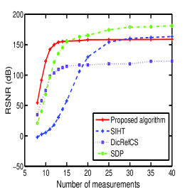
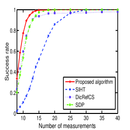
(a)	(b)

Figure 1: (a). RSNRs of respective algorithms vs. $M$; (b). Success rates of respective algorithms vs. $M$.

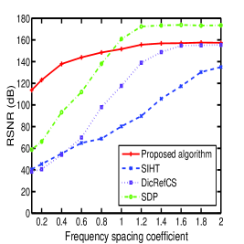
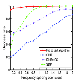
(a)	(b)

Figure 2: (a). RSNRs of respective algorithms vs. the frequency spacing coefficient $\mu$; (b). Success rates of respective algorithms vs. $\mu$.

IV Simulation Results

We now carry out experiments to illustrate the performance of our proposed algorithm and its comparison with other existing methods. We assume that the signal $\boldsymbol{u}\triangleq[u_{1}\phantom{0}\ldots\phantom{0}u_{L}]^{T}$ is a mixture of $K$ complex sinusoids, i.e.

$$u_{l}=\sum_{k=1}^{K}\alpha_{k}e^{-j\omega_{k}l}\qquad l=1,\ldots,L$$

with the frequencies $\{\omega_{k}\}$ uniformly generated over $[0,2\pi)$ and the amplitudes $\{\alpha_{k}\}$ uniformly distributed on the unit circle. The measurements $\boldsymbol{y}$ are obtained by randomly selecting $M$ entries from $L$ elements of $\boldsymbol{u}$. We first consider recovering the original signal $\boldsymbol{u}$ from the partial observations $\boldsymbol{y}$. The reconstruction accuracy is measured by the “reconstruction signal-to-noise ratio” (RSNR) which is defined as

$$\text{RSNR}=20\log_{10}\left(\frac{\|\boldsymbol{u}\|_{2}}{\|\boldsymbol{u}-\boldsymbol{\hat{u}}\|_{2}}\right)$$

We compare our proposed algorithm with the Bayesian dictionary refinement compressed sensing algorithm (denoted as DicRefCS) [8], the root-MUSIC based spectral iterative hard thresholding (SIHT) [7], and the atomic norm minimization via the semi-definite programming (SDP) approach [2]. Fig. 1(a) depicts the average RSNRs of respective algorithms as a function of the number of measurements, $M$, where we set $L=64$ and $K=3$. Results are averaged over $10^{3}$ independent runs, where the frequencies and the sampling indices (used to obtain $\boldsymbol{y}$) are randomly generated for each run. We observe that our proposed algorithm outperforms the other three methods in the region of a small $M$, where a gain of more than 15dB is achieved as compared with the DicRefCS and SDP methods. Our algorithm is surpassed by the SIHT and SDP methods as $M$ increases. Nevertheless, this performance improvement is of less significance since all methods provide quite decent recovery performance when $M$ is large.

The recovery performance is also evaluated in terms of the success rate. The success rate is computed as the ratio of the number of successful trials to the total number of independent runs, where $\{\alpha_{k}\}$ and $\{\omega_{k}\}$ are randomly generated for each run. Note that our algorithm and the DicRefCS method do not require the knowledge of the number of complex sinusoids, $K$. A trial is considered successful if the number of frequency components is estimated correctly and the estimation error between the estimated frequencies $\{\hat{\omega}_{k}\}$ and the true parameters $\{\omega_{k}\}$ is smaller than $10^{-3}$, i.e. $\frac{1}{2\pi}\|\boldsymbol{\omega}-\boldsymbol{\hat{\omega}}\|_{2}\leq 10^{-3}$. Fig. 1(b) depicts the success rates of respective algorithms vs. the number of measurements. This result again demonstrates the superiority of the proposed algorithm over other existing methods, particularly for the case when $M$ is small.

We examine the ability of our algorithm in resolving closely-spaced frequency components. The signal $\boldsymbol{u}$ is assumed a mixture of two complex sinusoids with the frequency spacing $d_{f}\triangleq\frac{1}{2\pi}(\omega_{1}-\omega_{2})$ equal to $\mu/L$, where $\mu$ is the frequency spacing coefficient ranging from $0.1$ to $2$. Fig. 2 shows RSNRs and success rates of respective algorithms vs. the frequency spacing coefficient $\mu$, where we set $L=64$ and $M=20$. Results are averaged over $10^{3}$ independent runs, with one of the two frequencies (the other frequency is determined by the frequency spacing) and the set of sampling indices randomly generated for each run. We see that our algorithm can accurately identify closely-spaced (say, $d_{f}=0.1/L$) frequencies with a high success rate and presents a significant performance advantage over other methods when two frequencies are very closely separated.

V Conclusions

We proposed an iterative reweighted algorithm for joint parametric dictionary learning and sparse signal recovery. The proposed algorithm was developed by iteratively decreasing a surrogate function majorizing the original objective function. Simulation results show that the proposed algorithm presents superiority over other existing methods in resolving closely-spaced frequency components.

References

- [1] E. Candès and C. Fernandez-Granda, “Towards a mathematical theory of super-resolution,” Communications on Pure and Applied Mathematics, to appear.
- [2] G. Tang, B. N. Bhaskar, B. Recht, and P. Shah, “Compressed sensing off the grid,” Available at http://arxiv.org/abs/1207.6053, 2012.
- [3] Y. Chi, L. L. Scharf, A. Pezeshki, and A. R. Calderbank, “Sensitivity to basis mismatch in compressed sensing,” IEEE Trans. Signal Processing, vol. 59, no. 5, pp. 2182–2195, May 2011.
- [4] Z. Yang, L. Xie, and C. Zhang, “Off-grid direction of arrival estimation using sparse Bayesian inference,” IEEE Trans. Signal Processing, vol. 61, no. 1, pp. 38–42, Jan. 2013.
- [5] L. Hu, J. Zhou, Z. Shi, and Q. Fu, “A fast and accurate reconstruction algorithm for compressed sensing of complex sinusoids,” IEEE Trans. Signal Processing, to appear.
- [6] A. Fannjiang and W. Liao, “Coherence pattern-guided compressive sensing with unresolved grids,” SIAM J. Imaging Sciences, vol. 5, no. 1, pp. 179–202, 2012.
- [7] M. F. Duarte and R. G. Baraniuk, “Spectral compressive sensing,” Applied and Computational Harmonic Analysis, vol. 35, pp. 111–129, 2013.
- [8] L. Hu, Z. Shi, J. Zhou, and Q. Fu, “Compressed sensing of complex sinusoids: An approach based on dictionary refinement,” IEEE Trans. Signal Processing, vol. 60, no. 7, pp. 3809–3822, 2012.
- [9] R. R. Coifman and M. Wickerhauser, “Entropy-based algorithms for best basis selction,” IEEE Trans. Information Theory, vol. IT-38, pp. 713–718, Mar. 1992.
- [10] I. F. Gorodnitsky and B. D. Rao, “Sparse signal reconstructions from limited data using focuss: A re-weighted minimum norm algorithm,” IEEE Trans. Signal Processing, vol. 45, no. 3, pp. 699–616, Mar. 1997.
- [11] E. Candès, M. Wakin, and S. Boyd, “Enhancing sparsity by reweighted minimization,” Journal of Fourier Analysis and Applications, vol. 14, pp. 877–905, Dec. 2008.
- [12] R. Chartrand and W. Yin, “Iterative reweighted algorithm for compressive sensing,” in IEEE International Conference on Acoustics, Speech, and Signal Processing, Las Vegas, Nevada, USA, 2008.
- [13] Y. Shen, J. Fang, and H. Li, “Exact reconstruction analysis of log-sum minimization for compressed sensing,” IEEE Signal Processing Letters, vol. 20, pp. 1223–1226, Dec. 2013.
- [14] M. Ataee, H. Zayyani, M. Babaie-Zadeh, and C. Jutten, “Parametric dictionary learning using steepest descent,” in IEEE International Conference on Acoustics, Speech, and Signal Processing, Proceedings, Dallas, Texas, USA, 2010.
- [15] K. Lange, D. Hunter, and I. Yang, “Optimization transfer using surrogate objective functions,” Journal of Computational and Graphical Statistics, vol. 9, no. 1, pp. 1–20, Mar. 2000.