Statics and dynamics of a binary dipolar Bose-Einstein condensate soliton

Abstract

We study the statics and dynamics of a binary dipolar Bose-Einstein condensate soliton for repulsive inter- and intraspecies contact interactions with the two components subject to different spatial symmetries $-$ distinct quasi-one-dimensional and quasi-two-dimensional shapes $-$ using numerical solution and variational approximation of a three-dimensional mean-field model. The results are illustrated with realistic values of parameters in the binary ¹⁶⁴Dy-¹⁶⁸Er mixture. The possibility of forming robust dipolar solitons of very large number of atoms make them of great experimental interest. The existence of the solitons is illustrated in terms of stability phase diagrams. Exotic shapes of these solitons are illustrated in isodensity plots. The variational results for statics (size and chemical potential) and dynamics (small oscillation) of the binary soliton compare well with the numerical results. A way of preparing and studying these solitons in laboratory is suggested.

1 Introduction

A bright soliton is a self-reinforcing solitary wave that travels at constant speed maintaining its shape, due to a cancellation of dispersive effect and nonlinear attraction. Matter-wave soliton and quasi-one-dimensional (quasi-1D) soliton train were created and investigated experimentally in Bose-Einstein condensate (BEC) of ⁷Li [1, 2] and ⁸⁵Rb atoms [3]. These quasi-1D solitons appear for attractive contact interaction in a axially-free BEC under radial harmonic trap [4].

The observation of BECs of ¹⁶⁴Dy [5, 6], ¹⁶⁸Er [7] and ⁵²Cr [8, 9, 10, 11, 12] atoms with large magnetic dipole moments has opened new directions of research in the study of BEC solitons. Polar molecules with much larger electric dipole moments are also being considered for BEC experiments [13]. In addition to the conventional quasi-1D solitons [14] of nondipolar BEC, one can have quasi-two-dimensional (quasi-2D) solitons in dipolar BEC [15]. More interestingly, one can have dipolar BEC solitons for fully repulsive contact interaction [14]. Moreover, solitons in dipolar BEC remain stable when the harmonic trap(s) is(are) replaced by periodic optical-lattice trap(s) in quasi-1D [16] and quasi-2D [17] configurations. Because of these interesting possibilities in dipolar BEC, we study here the formation of solitons in a binary dipolar BEC. Because of the complexity in dealing with the inter- and intraspecies dipolar interactions, there have been only a few studies of the binary dipolar mixture [18, 19]. We consider the numerical solution and variational approximation of a three-dimensional (3D) mean-field model in our study of binary dipolar BEC soliton where the atoms are polarized along $z$ axis.

There have been recent experimental [20] and theoretical [21] studies in binary BECs employing distinct trapping symmetry on each component. For example, the first component of the binary BEC could have a quasi-1D shape and the second component a quasi-2D shape, or one can have a quasi-2D-quasi-2D binary mixture with the first component lying in the $x-y$ plane and the second component in the $y-z$ plane. Hence, we will also consider distinct spatial symmetry of the two components in a binary dipolar BEC soliton, thus leading to exotic density profiles of the mixture. Among the distinct spatial symmetries of the binary dipolar BEC soliton, we consider (a) both components in quasi-1D shape along $z$ axis, (b) one component in quasi-2D shape in $y-z$ plane and the other in quasi-1D shape along $z$ axis, (c) both components in quasi-2D shape in $y-z$ plane, (d) one component in quasi-2D shape in $y-z$ plane and the other in quasi-2D shape in $x-z$ plane, and finally, (e) one component in quasi-2D shape in $x-y$ plane and the other in quasi-1D shape along $y$ axis. All these possibilities are realized for repulsive inter- and intraspecies contact interactions except the last one where we need attractive interspecies contact interaction for stability. This creates a new scenario for robust solitons of very large numer of atoms stabilized by short-range repulsion and long-range inter- and intraspecies dipolar attraction.

We illustrate our findings using realistic parameters in the ¹⁶⁴Dy-¹⁶⁸Er mixture. The stability of binary dipolar solitons is illustrated in phase diagrams involving critical number of atoms and interaction strengths. The profiles of the binary solitons are displayed in isodensity plots of the two components. The variational approximation to the sizes and chemical potentials of the two components is compared with the numerical solution of the mean-field model. The numerical study of breathing oscillation of the stable dipolar binary BEC soliton is found to be in reasonable agreement with a time-dependent variational model calculation.

In section 2 the mean-field model for the binary dipolar BEC soliton is developed. A time-dependent, analytic, Euler-Lagrange Gaussian variational approximation of the model is also presented. The results of numerical calculation are shown in section 3. Finally, in section 4 we present a brief summary of our findings.

2 Mean-field model for a binary dipolar BEC soliton

We consider a binary dipolar BEC soliton, interacting via inter- and intraspecies interactions, with the mass, number of atoms, magnetic dipole moment, and scattering length for the two species $i=1,2,$ denoted by $m_{i},N_{i},\widehat{\mu}_{i},a_{i},$ respectively. The inter- ($V_{12}$) and intraspecies ($V_{i}$) interactions for two atoms at positions $\bf r$ and $\bf r^{\prime}$ are taken as

$$V_{12}({\bf R})=\frac{\mu_{0}\widehat{\mu}_{1}\widehat{\mu}_{2}}{4\pi}\frac{1-3\cos^{2}\theta}{|{\bf R}|^{3}}+\frac{2\pi\hbar^{2}a_{12}}{m_{R}}\delta({\bf R}),$$ (1)

$$V_{i}({\bf R})=\frac{\mu_{0}\widehat{\mu}_{i}^{2}}{4\pi}\frac{1-3\cos^{2}\theta}{|{\bf R}|^{3}}+\frac{4\pi\hbar^{2}a_{i}}{m_{i}}\delta({\bf R}),$$ (2)

where $\bf R=r-r^{\prime},$ $\mu_{0}$ is the permeability of free space, $\theta$ is the angle made by the vector ${\bf R}$ with the polarization $z$ direction, $a_{12}$ is the intraspecies scattering length and $m_{R}=m_{1}m_{2}/(m_{1}+m_{2})$ is the reduced mass of the two species of atoms. With these interactions, the coupled Gross-Pitaevskii (GP) equations for the binary dipolar BEC can be written as [19]

$$\,{\mbox{i}}\hbar\frac{\partial\phi_{1}({\bf r},t)}{\partial t}={\Big{[}}-\frac{\hbar^{2}}{2m_{1}}\nabla^{2}+\frac{1}{2}m_{1}\omega_{1}^{2}(\nu_{1}x^{2}+\gamma_{1}y^{2}+\lambda_{1}z^{2})$$

$$+\frac{4\pi\hbar^{2}}{m_{1}}{a}_{1}N_{1}|\phi_{1}({\bf r},t)|^{2}+\frac{2\pi\hbar^{2}}{m_{R}}{a}_{12}N_{2}|\phi_{2}({\bf r},t)|^{2}+N_{1}\frac{\mu_{0}\ {\widehat{\mu}}^{2}_{1}}{4\pi}\int V_{dd}({\mathbf{R}})|\phi_{1}({\mathbf{r}^{\prime}},t)|^{2}d{\mathbf{r}}^{\prime}$$

$$+N_{2}\frac{\mu_{0}\ {\widehat{\mu}}_{1}\widehat{\mu}_{2}}{4\pi}\int V_{dd}({\mathbf{R}})|\phi_{2}({\mathbf{r}^{\prime}},t)|^{2}d{\mathbf{r}}^{\prime}{\Big{]}}\phi_{1}({\bf r},t),$$ (3)

$${\mbox{i}}\hbar\frac{\partial\phi_{2}({\bf r},t)}{\partial t}={\Big{[}}-\frac{\hbar^{2}}{2m_{2}}\nabla^{2}+\frac{1}{2}m_{2}\omega_{2}^{2}(\nu_{2}x^{2}+\gamma_{2}y^{2}+\lambda_{2}z^{2})$$

$$+\frac{4\pi\hbar^{2}}{m_{2}}{a}_{2}N_{2}|\phi_{2}({\bf r},t)|^{2}+\frac{2\pi\hbar^{2}}{m_{R}}{a}_{12}N_{1}|\phi_{1}({\bf r},t)|^{2}+N_{2}\frac{\mu_{0}\ {\widehat{\mu}}^{2}_{2}}{4\pi}\int V_{dd}({\mathbf{R}})|\phi_{2}({\mathbf{r}^{\prime}},t)|^{2}d{\mathbf{r}}^{\prime}$$

$$+N_{1}\frac{\mu_{0}\ {\widehat{\mu}}_{1}\widehat{\mu}_{2}}{4\pi}\int V_{dd}({\mathbf{R}})|\phi_{1}({\mathbf{r}^{\prime}},t)|^{2}d{\mathbf{r}}^{\prime}\Big{]}\phi_{2}({\bf r},t),$$ (4)

$$V_{dd}({\mathbf{R}})=\frac{1-3\cos^{2}\theta}{{\mathbf{R}}^{3}},\quad\rho^{2}=x^{2}+y^{2},\quad{\mbox{i}}=\sqrt{-1}.$$ (5)

Here $\omega_{i}$ are the frequencies of the traps and $\nu_{i},\gamma_{i},$ and $\lambda_{i}$ are trap anisotropy parameters.

To compare the dipolar and contact interactions, the intra- and interspecies dipolar interactions are expressed in terms of the dipolar lengths $a_{dd}^{(i)}$ and $a_{dd}^{(12)}$, defined by

$$a_{dd}^{(i)}=\frac{\mu_{0}\widehat{\mu}_{i}^{2}m_{i}}{12\pi\hbar^{2}},\quad a_{dd}^{(12)}=\frac{\mu_{0}\widehat{\mu}_{1}\widehat{\mu}_{2}m_{R}}{6\pi\hbar^{2}}.$$ (6)

We express the strengths of the dipolar interactions by these lengths and transform (3) and (2) into the following dimensionless form [19]

$$\,{\mbox{i}}\frac{\partial\phi_{1}({\bf r},t)}{\partial t}={\Big{[}}-\frac{\nabla^{2}}{2}+\frac{1}{2}(\nu_{1}x^{2}+\gamma_{1}y^{2}+\lambda_{1}z^{2})$$

$$\,+g_{1}|\phi_{1}|^{2}+g_{12}|\phi_{2}|^{2}+g_{dd}^{(1)}\int V_{dd}({\mathbf{R}})|\phi_{1}({\mathbf{r}^{\prime}},t)|^{2}d{\mathbf{r}}^{\prime}$$

$$\,+g_{dd}^{(12)}\int V_{dd}({\mathbf{R}})|\phi_{2}({\mathbf{r}^{\prime}},t)|^{2}d{\mathbf{r}}^{\prime}{\Big{]}}\phi_{1}({\bf r},t),$$ (7)

$$\,{\mbox{i}}\frac{\partial\phi_{2}({\bf r},t)}{\partial t}={\Big{[}}-m_{12}\frac{\nabla^{2}}{2}+\frac{1}{2}m_{\omega}(\nu_{2}x^{2}+\gamma_{2}y^{2}+\lambda_{2}z^{2})$$

$$\,+g_{2}|\phi_{2}|^{2}+g_{21}|\phi_{1}|^{2}+g_{dd}^{(2)}\int V_{dd}({\mathbf{R}})|\phi_{2}({\mathbf{r}^{\prime}},t)|^{2}d{\mathbf{r}}^{\prime}$$

$$\,+g_{dd}^{(21)}\int V_{dd}({\mathbf{R}})|\phi_{1}({\mathbf{r}^{\prime}},t)|^{2}d{\mathbf{r}}^{\prime}{\Big{]}}\phi_{2}({\bf r},t),$$ (8)

where $m_{\omega}=\omega_{2}^{2}/(m_{12}\omega_{1}^{2}),$ $m_{12}={m_{1}}/{m_{2}},$ $g_{1}=4\pi a_{1}N_{1},$ $g_{2}=4\pi a_{2}N_{2}m_{12},$ $g_{12}={2\pi m_{1}}a_{12}N_{2}/m_{R},$ $g_{21}={2\pi m_{1}}a_{12}N_{1}/m_{R},$ $g_{dd}^{(2)}=3N_{2}a_{dd}^{(2)}m_{12},$ $g_{dd}^{(1)}=3N_{1}a_{dd}^{(1)},$ $g_{dd}^{(12)}=3N_{2}a_{dd}^{(12)}m_{1}/2m_{R},$ $g_{dd}^{(21)}=3N_{1}a_{dd}^{(12)}m_{1}/2m_{R}.$ In (7) and (8), length is expressed in units of oscillator length $l_{0}=\sqrt{\hbar/(m_{1}\omega_{1})}$, energy in units of oscillator energy $\hbar\omega_{1}$, density $|\phi_{i}|^{2}$ in units of $l_{0}^{-3}$, and time in units of $t_{0}=1/\omega_{1}$.

Convenient analytic variational approximation to (7) and (8) can be obtained with the following ansatz for the wave functions in case of axially symmetric traps with $\nu_{i}=\gamma_{i}=1$: [22, 23, 24]

$$\phi_{i}({\bf r},t)=\frac{\pi^{-3/4}}{w_{\rho i}\sqrt{w_{zi}}}\exp\Big{[}-\frac{\rho^{2}}{2w_{\rho i}^{2}}-\frac{z^{2}}{2w_{zi}^{2}}+\mathrm{i}\alpha_{i}\rho^{2}+\mathrm{i}\beta_{i}z^{2}\Big{]}$$ (9)

where ${\bf r}=\{\vec{\rho},z\},{\vec{\rho}}=\{x,y\}$, $w_{\rho i}$ and $w_{zi}$ are the widths and $\alpha_{i}$ and $\beta_{i}$ are additional variational parameters. The effective Lagrangian for the binary system is [24]

$$L=\int d{\bf r}\frac{1}{2}\Big{[}\sum_{i}\Big{\{}{\mathrm{i}}N_{i}(\phi_{i}\dot{\phi}_{i}^{*}-\phi_{i}^{*}\dot{\phi}_{i})+N_{i}g_{i}|\phi_{i}({\bf r})|^{4}\Big{\}}+N_{1}[\rho^{2}+\lambda_{1}z^{2}]|\phi_{1}({\bf r})|^{2}$$

$$+N_{2}[\rho^{2}+\lambda_{2}z^{2}]|\phi_{2}({\bf r})|^{2}m_{\omega}+N_{1}|\nabla\phi_{1}({\bf r})|^{2}+m_{12}N_{2}|\nabla\phi_{2}({\bf r})|^{2}+2N_{1}g_{12}|\phi_{1}({\bf r})|^{2}|\phi_{2}({\bf r})|^{2}\Big{]}$$

$$+\int\int d{\bf r}^{\prime}d{\bf r}\Big{[}\sum_{i}\frac{N_{i}}{2}g_{dd}^{(i)}V_{dd}({\bf R})|\phi_{i}({\bf r^{\prime}})|^{2}|\phi_{i}({\bf r})|^{2}+{N_{1}}g_{dd}^{(12)}V_{dd}({\bf R})|\phi_{1}({\bf r^{\prime}})|^{2}|\phi_{2}({\bf r})|^{2}\Big{]},$$ (10)

$$=\sum_{i=1}^{2}\frac{N_{i}}{2}(2w_{\rho i}^{2}\dot{\alpha}_{i}+w_{zi}^{2}\dot{\beta}_{i})+N_{1}\left[\frac{w_{\rho 1}^{2}}{2}+\frac{\lambda_{1}w_{z1}^{2}}{4}\right]+m_{\omega}N_{2}\left[\frac{w_{\rho 2}^{2}}{2}+\frac{\lambda_{2}w_{z2}^{2}}{4}\right]$$

$$+\frac{N_{1}}{2}\biggr{[}\frac{1}{w_{\rho 1}^{2}}+\frac{1}{2w_{z1}^{2}}+4w_{\rho 1}^{2}\alpha_{1}^{2}+2w_{z1}^{2}\beta_{1}^{2}\biggr{]}+\frac{N_{2}m_{12}}{2}\biggr{[}\frac{1}{w_{\rho 2}^{2}}+\frac{1}{2w_{z2}^{2}}+4w_{\rho 2}^{2}\alpha_{2}^{2}+2w_{z2}^{2}\beta_{2}^{2}\biggr{]}$$

$$+\frac{N_{1}^{2}[a_{1}-a_{dd}^{(1)}f(\kappa_{1})]}{\sqrt{2\pi}w_{\rho 1}^{2}w_{z1}}+\frac{N_{2}^{2}m_{12}[a_{2}-a_{dd}^{(2)}f(\kappa_{2})]}{\sqrt{2\pi}w_{\rho 2}^{2}w_{z2}}+\frac{2m_{1}N_{1}N_{2}[a_{12}-a_{dd}^{(12)}f(\kappa_{3})]}{\sqrt{\pi}m_{R}w_{\rho 3}^{2}w_{z3}},\quad$$ (11)

$$f(\kappa)=\frac{1+2\kappa^{2}-3\kappa^{2}d(\kappa)}{1-\kappa^{2}},\quad d(\kappa)=\frac{\mathrm{atan}(\sqrt{\kappa^{2}-1})}{\sqrt{\kappa^{2}-1}},$$

where $\kappa_{i}=w_{\rho i}/w_{zi},w_{\rho 3}=\sqrt{w_{\rho 1}^{2}+w_{\rho 2}^{2}}$ , $w_{z3}=\sqrt{w_{z1}^{2}+w_{z2}^{2}}$. In these equations the overhead dot denotes time derivative.

The Euler-Lagrange variational equations for the widths for the effective Lagrangian (2), obtained in usual fashion [24], can be written as

$$\ddot{w}_{\rho 1}=-\omega_{\rho 1}+\frac{1}{w_{\rho 1}^{3}}+\frac{N_{1}[2a_{1}-a_{dd}^{(1)}g(\kappa_{1})]}{\sqrt{2\pi}w_{\rho 1}^{3}w_{z1}}+\frac{2m_{1}N_{2}w_{\rho 1}[2a_{12}-a_{dd}^{(12)}g(\kappa_{3})]}{\sqrt{\pi}m_{R}w_{\rho 3}^{4}w_{z3}},$$ (12)

$$\ddot{w}_{z1}=-\lambda_{1}\omega_{z1}+\frac{1}{w_{z1}^{3}}+\frac{2N_{1}[a_{1}-a_{dd}^{(1)}h(\kappa_{1})]}{\sqrt{2\pi}w_{\rho 1}^{2}w_{z1}^{2}}+\frac{{{4}}m_{1}N_{2}w_{z1}[a_{12}-a_{dd}^{(12)}h(\kappa_{3})]}{\sqrt{\pi}m_{R}w_{\rho 3}^{2}w_{z3}^{3}},$$ (13)

$$\ddot{w}_{\rho 2}=-m_{\omega}\omega_{\rho 2}+\frac{m_{12}}{w_{\rho 2}^{3}}+\frac{N_{2}m_{12}[2a_{2}-a_{dd}^{(2)}g(\kappa_{2})]}{\sqrt{2\pi}w_{\rho 2}^{3}w_{z2}}+\frac{2m_{1}N_{1}w_{\rho 2}[2a_{12}-a_{dd}^{(12)}g(\kappa_{3})]}{\sqrt{\pi}m_{R}w_{\rho 3}^{4}w_{z3}},$$ (14)

$$\ddot{w}_{z2}=-m_{\omega}\lambda_{2}\omega_{z2}+\frac{m_{12}}{w_{z2}^{3}}+\frac{2N_{2}m_{12}[a_{2}-a_{dd}^{(2)}h(\kappa_{2})]}{\sqrt{2\pi}w_{\rho 2}^{2}w_{z2}^{2}}+\frac{{{4}}m_{1}N_{1}w_{z2}[a_{12}-a_{dd}^{(12)}h(\kappa_{3})]}{\sqrt{\pi}m_{R}w_{\rho 3}^{2}w_{z3}^{3}},$$ (15)

$$g(\kappa)=\frac{2-7\kappa^{2}-4\kappa^{4}+9\kappa^{4}d(\kappa)}{(1-\kappa^{2})^{2}},$$ (16)

$$h(\kappa)=\frac{1+10\kappa^{2}-2\kappa^{4}-9\kappa^{2}d(\kappa)}{(1-\kappa^{2})^{2}}.$$ (17)

The solution of the time-dependent equations (12) $-$ (15) gives the dynamics of the variational approximation.

The energy of the system is given by

$$E=N_{1}\left[\frac{w_{\rho 1}^{2}}{2}+\frac{\lambda_{1}w_{z1}^{2}}{4}\right]+m_{\omega}N_{2}\left[\frac{w_{\rho 2}^{2}}{2}+\frac{\lambda_{2}w_{z2}^{2}}{4}\right]+\frac{N_{1}}{2}\biggr{[}\frac{1}{w_{\rho 1}^{2}}+\frac{1}{2w_{z1}^{2}}\biggr{]}$$

$$+\frac{N_{2}m_{12}}{2}\biggr{[}\frac{1}{w_{\rho 2}^{2}}+\frac{1}{2w_{z2}^{2}}\biggr{]}+\frac{N_{1}^{2}[a_{1}-a_{dd}^{(1)}f(\kappa_{1})]}{\sqrt{2\pi}w_{\rho 1}^{2}w_{z1}}+\frac{N_{2}^{2}m_{12}[a_{2}-a_{dd}^{(2)}f(\kappa_{2})]}{\sqrt{2\pi}w_{\rho 2}^{2}w_{z2}}$$

$$+\frac{2m_{1}N_{1}N_{2}[a_{12}-a_{dd}^{(12)}f(\kappa_{3})]}{\sqrt{\pi}m_{R}w_{\rho 3}^{2}w_{z3}}.$$ (18)

The energy is actually the stationary (time-independent) part of the Lagrangian (2).

If $\mu_{i}$ is the chemical potential with which the stationary wave function $\phi_{i}({\bf r},t)$ propagates in time, e.g. $\phi_{i}({\bf r},t)\sim\exp(-i\mu_{i}t)\phi_{i}({\bf r})$, then the variational estimate for $\mu_{i}(\equiv\partial E/\partial N_{i})$ is:

$$\mu_{1}=\frac{\partial E}{\partial N_{1}}=\frac{1}{2}\biggr{[}\frac{1}{w_{\rho 1}^{2}}+\frac{1}{2w_{z1}^{2}}\biggr{]}+\left[\frac{w_{\rho 1}^{2}}{2}+\frac{\lambda_{1}w_{z1}^{2}}{4}\right]$$

$$+\frac{2N_{1}[a_{1}-a_{dd}^{(1)}f(\kappa_{1})]}{\sqrt{2\pi}w_{\rho 1}^{2}w_{z1}}+\frac{2m_{1}N_{2}[a_{12}-a_{dd}^{(12)}f(\kappa_{3})]}{\sqrt{\pi}m_{R}w_{\rho 3}^{2}w_{z3}},$$ (19)

$$\mu_{2}=\frac{\partial E}{\partial N_{2}}=\frac{m_{12}}{2}\biggr{[}\frac{1}{w_{\rho 2}^{2}}+\frac{1}{2w_{z2}^{2}}\biggr{]}+m_{\omega}\left[\frac{w_{\rho 2}^{2}}{2}+\frac{\lambda_{2}w_{z2}^{2}}{4}\right]$$

$$+\frac{2N_{2}m_{12}[a_{2}-a_{dd}^{(2)}f(\kappa_{2})]}{\sqrt{2\pi}w_{\rho 2}^{2}w_{z2}}+\frac{2m_{1}N_{1}[a_{12}-a_{dd}^{(12)}f(\kappa_{3})]}{\sqrt{\pi}m_{R}w_{\rho 3}^{2}w_{z3}}.$$ (20)

The widths of the stationary binary dipolar soliton can be obtained from the solution of (12) $-$ (15) setting the time derivatives of the widths to zero. This procedure is equivalent to a minimization of the energy (2), provided the stationary binary soliton is stable and corresponds to a energy minimum. In section 3, we will consider diverse types of anisotropic binary solitons. However, the Gaussian variational approximation above is applicable to only the conventional cigar-shaped axially-symmetric solitons with trap parameters $\nu_{i}=\gamma_{i}=1$ and $\lambda_{i}=0$.

3 Numerical Results

We perform numerical calculation for the stability and dynamics of the binary dipolar soliton using realistic values of atom numbers and interaction parameters in the ¹⁶⁴Dy-¹⁶⁸Er mixture. The ¹⁶⁴Dy and ¹⁶⁸Er atoms have the largest magnetic moments of all the dipolar atoms used in BEC experiments. The ¹⁶⁴Dy atoms are labeled $i=1$ and the ¹⁶⁸Er atoms are labeled $i=2$. The ¹⁶⁴Dy atoms have a large magnetic dipole moment $\widehat{\mu}_{1}=10\mu_{B}$ [6] with $\mu_{B}$ $(=9.27402\times 10^{-24}$ Am²) the Bohr magneton corresponding to the dipolar length $a_{dd}^{(1)}\equiv\mu_{0}\widehat{\mu}_{1}^{2}m_{1}/(12\pi\hbar^{2})\approx 132.7a_{0}$, with $a_{0}$ $(=5.29\times 10^{-11}$ m) the Bohr radius, $\mu_{0}=4\pi\times 10^{-7}$ N/A${}^{2},$ $\hbar=1.05457\times 10^{-34}$ m²kg/s, 1 amu $=1.66054\times 10^{-27}$ kg. For ¹⁶⁸Er atoms, $\widehat{\mu}_{2}=7\mu_{B}$ [7], the dipolar length $a_{dd}^{(2)}\equiv\mu_{0}\widehat{\mu}_{2}^{2}m_{2}/(12\pi\hbar^{2})\approx 66.6a_{0}$, and the interspecies dipolar length $a_{dd}^{(12)}\equiv\mu_{0}\widehat{\mu}_{1}\widehat{\mu}_{2}m_{R}/(6\pi\hbar^{2})\approx 94.0a_{0}$. Thus the dipolar interaction in ¹⁶⁴Dy atoms is more than eight times larger than that in ⁵²Cr atoms with a dipolar length $a_{dd}\approx 15a_{0}$ [9, 11].

The contribution of the dipolar interaction is calculated in momentum space by Fourier transformation (FT) and the following convolution integral [23]

$$\int d{\bf r}V_{dd}({\bf r-r^{\prime}})n({\bf r^{\prime}})=\int\frac{d{\bf k}}{(2\pi)^{3}}e^{i{\bf k}\cdot{\bf r}}\tilde{V}_{dd}(\bf k)\tilde{n}({\bf k}),$$ (21)

$$\tilde{V}_{dd}({\bf k})=\frac{4\pi}{3}\left[\frac{3k_{z}^{2}}{{\bf k}^{2}}-1\right],$$ (22)

with density $n({\bf r})=|\phi({\bf r})|^{2}$. The FT is defined by

$$\tilde{A}({\bf k})=\int d{\bf r}A({\bf r})e^{i{\bf k}\cdot{\bf r}},$$ (23)

$$A({\bf r})=\int\frac{d{\bf k}}{(2\pi)^{3}}\tilde{A}({\bf k})e^{-i{\bf k}\cdot{\bf r}}.$$ (24)

The FT $\tilde{n}({\bf k})$ of density and the inverse FT are calculated numerically by a fast FT routine. The whole procedure is performed in a 3D Cartesian coordinate system irrespective of the underlying trap symmetry. We solve (7) and (8) by the split-step Crank-Nicolson discretization scheme using a space step of $\sim 0.1-0.2$ and the time step $\sim 0.001-0.003$ [23, 25].

We will be studying the binary solitons in different trap symmetries mostly for repulsive interspecies and intraspecies contact interactions. The attraction for the formation of the solitons will be provided by the long-range dipolar interactions. These repulsive contact interactions will make the collapse more difficult and will generate robust binary dipolar solitons. This will allow us to consider binary solitons in a new scenario, which is not possible in a nondipolar BEC. However, that a net attraction for the formation of soliton is available in the binary system, we take the dipolar length scales larger than the corresponding atomic scattering lengths: $a_{dd}^{(i)}>a_{i},a_{dd}^{(12)}>a_{12}$. If these conditions are satisfied the net nonlinear interaction turns to be attractive in an axially free set up as can be realized from (2). In the present study we take for the ¹⁶⁴Dy atoms $a_{1}=120a_{0}$, and for the ¹⁶⁸Er atoms $a_{2}=60a_{0}$. The yet unknown interspecies scattering length $a_{12}$ is taken as a variable. Of these, the scattering length $a_{1}$ of ¹⁶⁴Dy atoms is close to the experimental value [6]. The scattering lengths $a_{2}$ and $a_{12}$ can be controlled by independent magnetic [26] and optical Feshbach resonance [27] techniques. We consider the trap frequencies $\omega_{1}=\omega_{2}=2\pi\times 61$ Hz, so that the length scale $l_{0}\equiv\sqrt{\hbar/m_{1}\omega_{1}}=1$ $\mu$m, and the constant $m_{\omega}=1/m_{12}$ in (8).

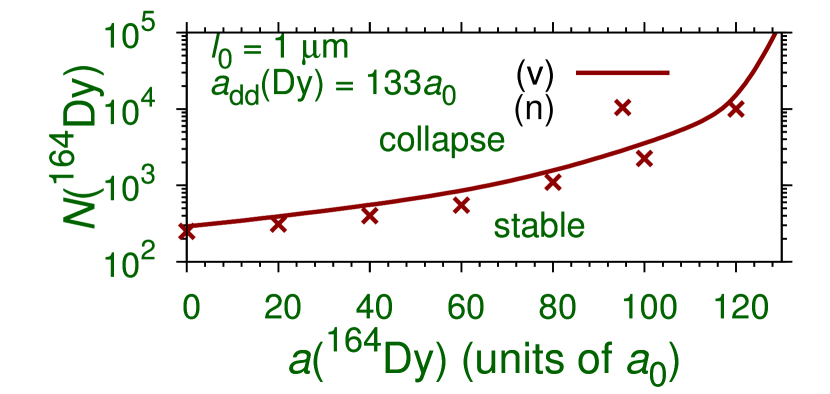
Figure 1: Stability phase diagram for a single-component ¹⁶⁴Dy soliton free to move along the axial $z$ direction for a harmonic trap $\rho^{2}/2$ in the $x-y$ plane as obtained from numerical calculation (n) and variational approximation (v). The oscillator length $l_{0}=1$ $\mu$m, $a_{dd}$(Dy)=$132.7a_{0}$.

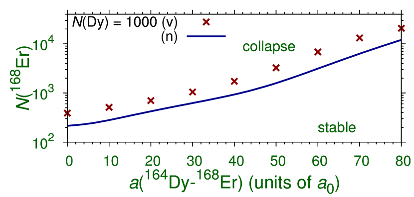
Figure 2: Stability phase plot for a binary ¹⁶⁴Dy-¹⁶⁸Er soliton free to move along the axial $z$ direction with the axially-symmetric trap $\rho^{2}/2$ in the $x-y$ plane on both components as obtained from numerical calculation (n) and variational approximation (v). The parameters employed are $a$(Dy)$=120a_{0},a$(Er)$=60a_{0},a_{dd}$(Dy)$=132.7a_{0},a_{dd}$(Er)$=66.6a_{0},a_{dd}$(Dy-Er)$=94a_{0}$, $l_{0}=1$ $\mu$m and $m_{\omega}=1/m_{12}$.

Figure 3: Numerically obtained stability phase diagram for a binary quasi-2D ¹⁶⁴Dy-¹⁶⁸Er soliton free to move in the $y-z$ plane with the harmonic trap $x^{2}/2$ on both components. All parameters are the same as in figure 2.

First we study the stability of a single-component ¹⁶⁴Dy soliton harmonically trapped in the $x-y$ plane by the potential $\rho^{2}/2$ and free to move in the $z$ direction. The result is shown in figure 1 where we display the critical number of atoms $N$(Dy) versus the atomic scattering length $a$(Dy) as obtained from the Gaussian variational approximation and the complete numerical solution. The variational energies are larger than the numerical energies and the variational states are loosely bound compared the numerical states. Consequently, the variational states can accommodate more dipolar atoms in a stable dipolar soliton as seen in figure 1.

Now we study the stability of a binary ¹⁶⁴Dy-¹⁶⁸Er soliton free to move in the $z$ direction while both components are harmonically trapped in the $x-y$ plane by the potential $\rho^{2}/2$. Both numerical and variational results are shown in figure 2 for the number of ¹⁶⁴Dy atoms $N$(Dy) = 1000. In this figure we plot the critical number of ¹⁶⁸Er atoms $N$(Er) in the stable binary soliton versus the interatomic scattering length $a$(Dy-Er). As in the single-component case, the variational critical number of ¹⁶⁸Er atoms in the binary soliton is larger than the numerical critical number of the same.

In the above examples we considered only the soliton(s) with an axially-symmetric trap in the $x-y$ plane. In case of single-component dipolar soliton, the axial symmetry can be removed by taking only a harmonic or optical-lattice (OL) trap along the $x$ direction, thus generating an asymmetric two-dimensional soliton free to move in the $y-z$ plane [15]. In case of binary dipolar solitons the axial symmetry of the trap acting on one or both components can be removed, thus generating a new class of asymmetric binary solitons. One example of such asymmetric binary soliton is obtained by considering the harmonic trap $x^{2}/2$ on both components. In this case both component solitons ¹⁶⁴Dy and ¹⁶⁸Er are clearly asymmetric. A stability phase diagram in this case is shown in figure 3 for 1000 ¹⁶⁴Dy atoms, where we plot the critical number $N$(Er) of ¹⁶⁸Er atoms in a stable binary soliton versus the interspecies scattering length $a$(Dy-Er). In the following we will also consider few examples of binary dipolar solitons with other types of traps.

In figures 2 and 3 we have considered different types of traps to achieve the binary dipolar soliton. As the number of traps on the binary soliton is reduced the solitons become loosely bound thus accommodating more atoms. The increase of the number of traps makes the binary soliton more compact and thus vulnerable to collapse due to strong dipolar interaction. The binary soliton of figure 2 is most compact with four 1D traps, that figure 3 has two 1D traps. Consequently, for the fixed number $N$(Dy) = 1000 of ¹⁶⁴Dy atoms, the critical number of numerically obtained ¹⁶⁸Er atoms is smaller in figure 2 compared to those in figure 3.

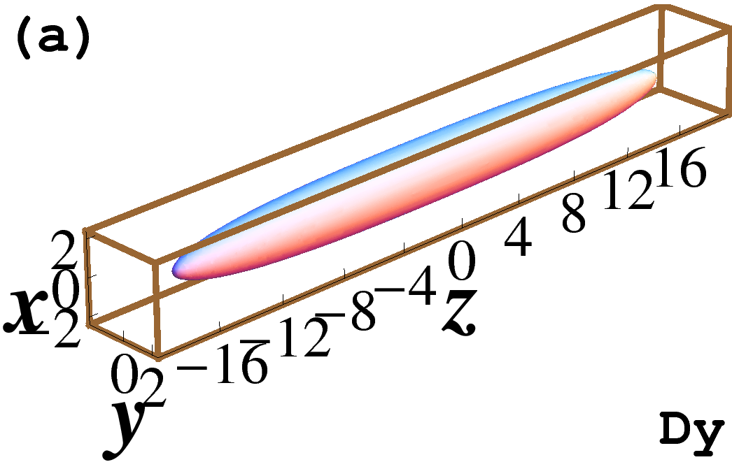
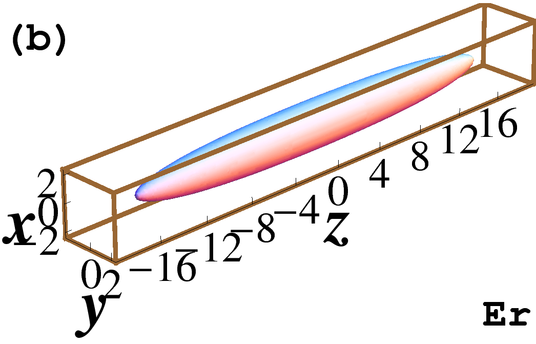
Figure 4: Isodensity plots of numerically obtained (a) ¹⁶⁴Dy and (b) ¹⁶⁸Er profiles of a binary cigar-shaped ¹⁶⁴Dy-¹⁶⁸Er soliton of 1000 atoms each, with the radial trap $\rho^{2}/2$ on both components, and free to move along the $z$ direction. All parameters are the same as in figure 2 except the interspecies scattering length $a$(Dy-Er) = $70a_{0}$. Lengths are in units of $l_{0}(\equiv 1$ $\mu$m) and density in units of $l_{0}^{-3}$. The density on contour is 0.001.

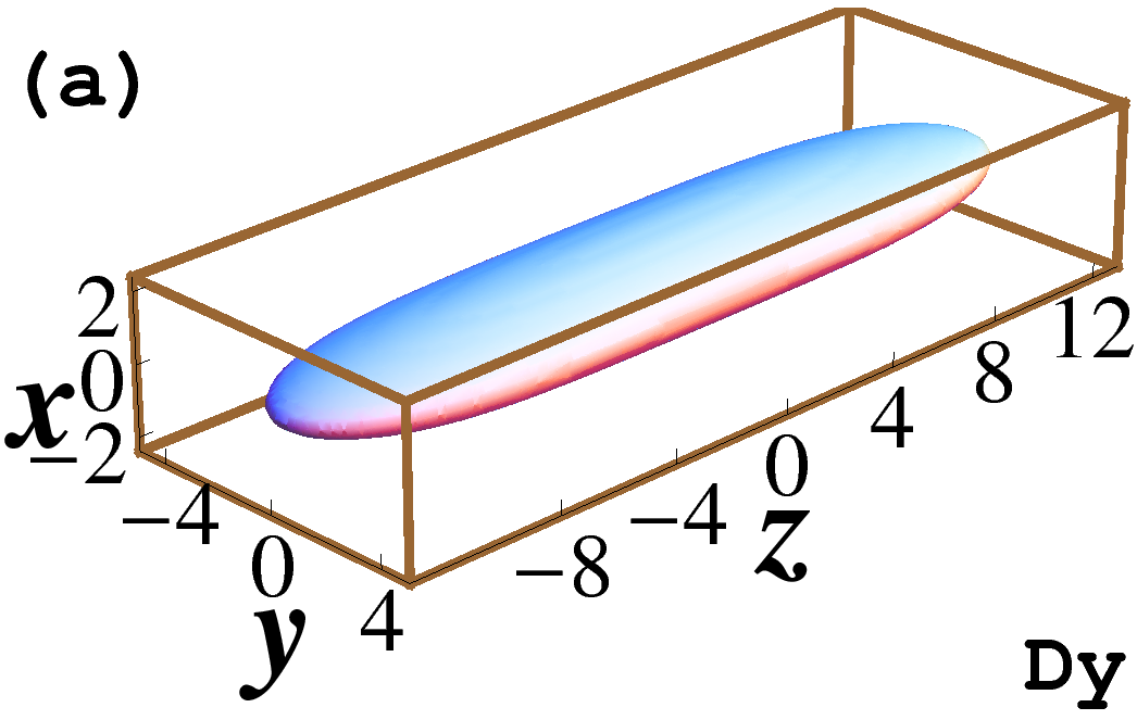
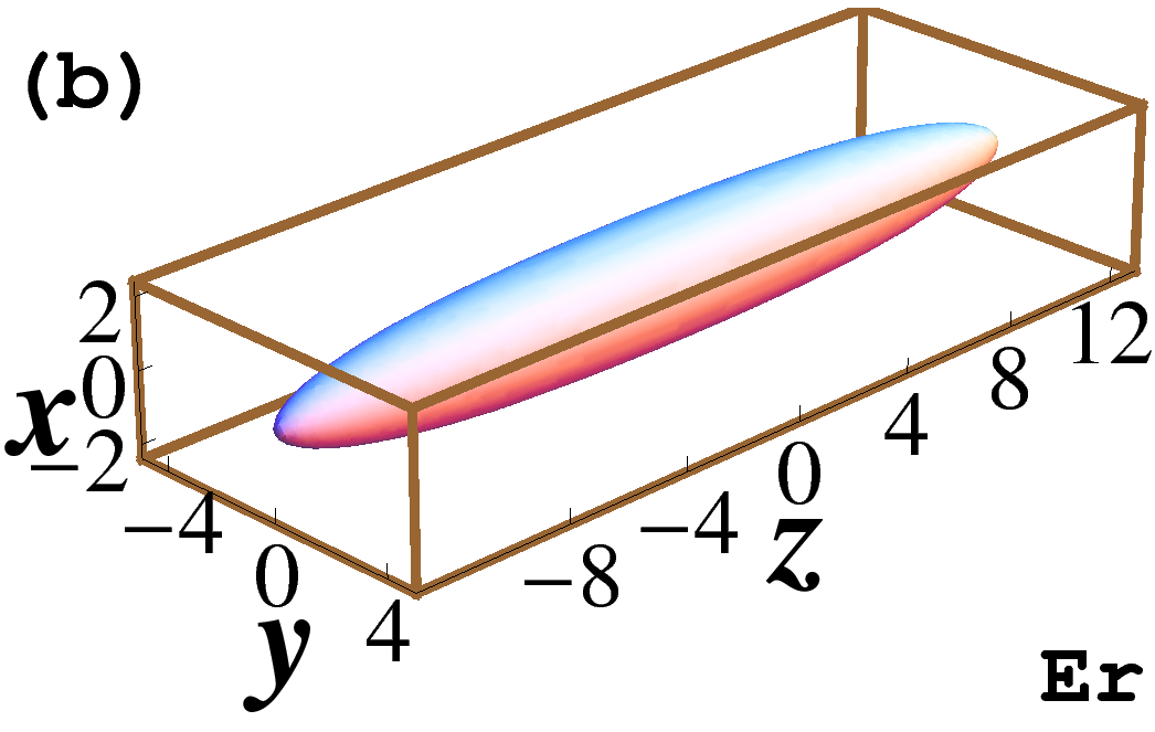
Figure 5: Isodensity plots of numerically obtained (a) ¹⁶⁴Dy and (b) ¹⁶⁸Er profiles of a binary ¹⁶⁴Dy-¹⁶⁸Er soliton of 1000 atoms each and free to move along the $z$ direction. The first component (Dy), subject to a harmonic trap $x^{2}/2$, has a quasi-2D profile in $y-z$ plane whereas the second component (Er) with the trap $\rho^{2}/2$ has a quasi-1D profile along $z$ axis. All parameters are the same as in figure 2 except the interspecies scattering length $a$(Dy-Er) = $50a_{0}$. The density on contour is 0.001.

The numerically obtained profiles of different types of binary dipolar solitons are next illustrated by their isodensity contours. First we consider the axially-symmetric binary soliton with the axially-symmetric trap $\rho^{2}/2$ acting on both components and free to move along the $z$ direction. The corresponding isodensity profiles of the two components are shown in Figs. 4 (a) and (b) for 1000 ¹⁶⁴Dy and 1000 ¹⁶⁸Er atoms, respectively. The solitons have axially-symmetric cigar shapes. Next we consider an asymmetric binary dipolar soliton with the harmonic 1D trap $x^{2}/2$ on the first component (Dy) and the axially-symmetric trap $\rho^{2}/2$ on the second component (Er). The corresponding isodensity profiles of the two components are shown in Figs. 5 (a) and (b).

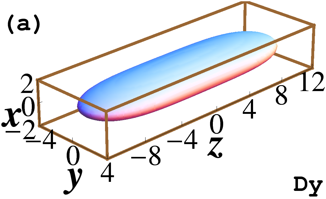
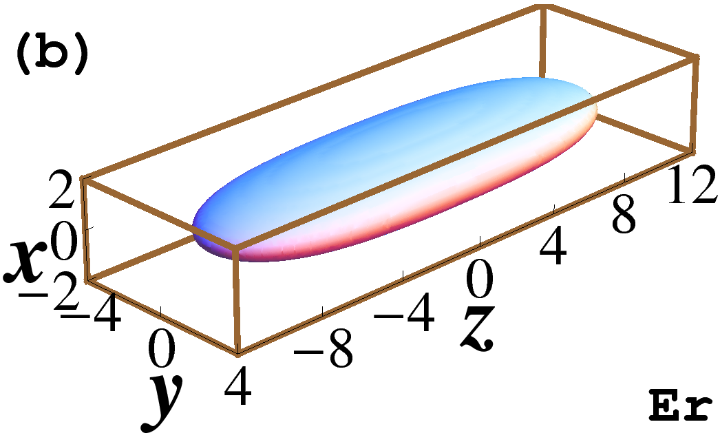
Figure 6: Isodensity plots of numerically obtained (a) ¹⁶⁴Dy and (b) ¹⁶⁸Er profiles of a binary ¹⁶⁴Dy-¹⁶⁸Er soliton of 1000 atoms each and free to move in the $y-z$ plane. Both components, subject to the harmonic trap $x^{2}/2$, have a quasi-2D profile in $y-z$ plane. All parameters are the same as in figure 2 except the interspecies scattering length $a$(Dy-Er) = $30a_{0}$. The density on contour is 0.001.

Now we consider the shape of binary dipolar soliton with asymmetric traps on each of the two components. The easiest way to achieve this is to apply the asymmetric trap $x^{2}/2$ on each of the components. Such a binary soliton is free to move in the $y-z$ plane. Because of the only trap in the $x$ direction it is thin in this direction and has a large size in the $y-z$ plane. The extension along the polarization $z$ direction is the largest as the aligned dipoles along this direction lead to a natural elongation along this direction for large dipolar interaction, as clearly demonstrated in figures 1 and 3 of [9], where it is experimentally observed that an increase of the dipolar parameter $a_{dd}/a$ leads to an elongation of the BEC along the polarization $z$ direction. The change in the dipolar parameter was achieved by changing the scattering length $a$ by the Feshbach resonance technique [26]. The profiles of the 1000 ¹⁶⁴Dy and the 1000 ¹⁶⁸Er atoms in this binary soliton are quite similar and are illustrated in figures 6 (a) and (b), respectively, for the ¹⁶⁴Dy and ¹⁶⁸Er components.

The binary solitons considered so far have a qualitatively similar shape for the two components and hence they are best illustrated in two different plots. Next we consider two more types of asymmetric binary solitons which lead to very distinct profiles for the two components. In these cases, in addition to distinct plot for the two components, it is also illustrative to plot the isodensity profiles of the binary soliton. First we consider an asymmetric harmonic trap $x^{2}/2$ on the first component (Dy) and an asymmetric trap $y^{2}/2$ on the second component (Er). The binary soliton is free to move in the $z$ direction with the quasi-2D profile of the first component lying in the $y-z$ plane and the quasi-2D profile of the second component lying in the $x-z$ plane. Again due to the aligned dipoles in the polarization $z$ direction the binary soliton has the largest spatial extension along this direction. The isodensity contour of the two components and of the binary soliton are illustrated in figures 7 (a), (b), and (c), respectively.

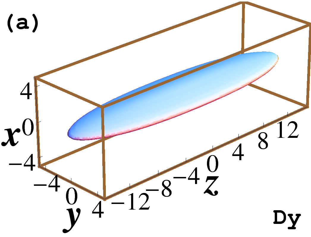
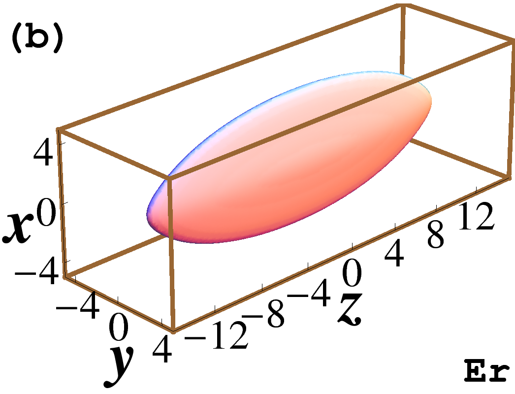
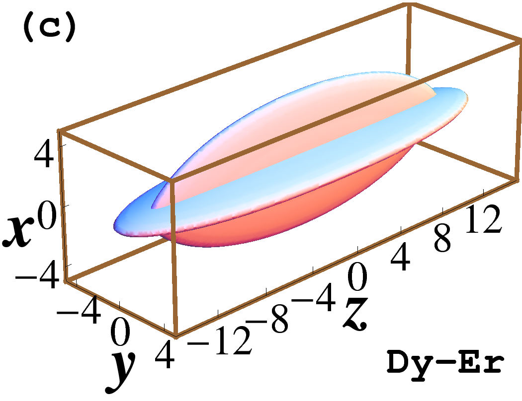
Figure 7: Isodensity plots of numerically obtained (a) ¹⁶⁴Dy and (b) ¹⁶⁸Er and (c) ¹⁶⁴Dy-¹⁶⁸Er profiles of a binary ¹⁶⁴Dy-¹⁶⁸Er soliton of 1000 atoms each and free to move in the $z$ direction. The first component (Dy), subject to a harmonic trap $x^{2}/2$, has a quasi-2D profile in $y-z$ plane whereas the second component (Er) with the trap $y^{2}/2$ has a quasi-2D profile in the $x-z$ plane. All parameters are the same as in figure 2 except the interspecies scattering length $a$(Dy-Er) = $20a_{0}$. The density on contour is 0.001.

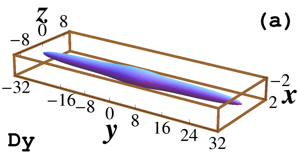
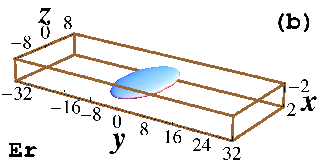
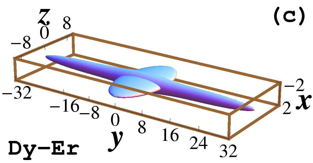
Figure 8: Isodensity plots of numerically obtained (a) ¹⁶⁴Dy and (b) ¹⁶⁸Er and (c) ¹⁶⁴Dy-¹⁶⁸Er profiles of a binary ¹⁶⁴Dy-¹⁶⁸Er soliton of 200 ¹⁶⁴Dy atoms and 1000 ¹⁶⁸Er atoms free to move in the $y$ direction. The first component (Dy), subject to a harmonic trap $(x^{2}+z^{2})/2$, has a quasi-1D profile along $y$ direction whereas the second component (Er) with the trap $x^{2}/2$ has a quasi-2D profile in the $y-z$ plane. All parameters are the same as in figure 2 except the interspecies scattering length $a$(Dy-Er) = $-40a_{0}$. The density on contour is 0.001.

The binary solitons considered so far have repulsive interspecies and intraspecies contact interactions. These solitons are solely confined by the dipolar interaction. Now we consider a new class of binary soliton stabilized by attractive interspecies contact interaction. In this case the first component ¹⁶⁴Dy is subject to the harmonic trap $(x^{2}+z^{2})/2$ and the second component ¹⁶⁸Er is subject to the trap $x^{2}/2$. The interspecies scattering length is set at $a$(Dy-Er)$=-40a_{0}$. The shapes of the two components are quite distinct in this case. The isodensity profiles of ¹⁶⁴Dy and ¹⁶⁸Er are shown in figures 8 (a) and (b) and that of the binary overlapping soliton is illustrated in figure 8 (c).

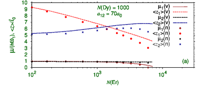
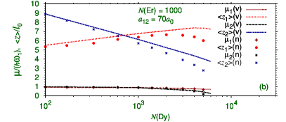
Figure 9: Variational (v) and numerical (n) results for chemical potential $\mu_{i}$ and rms size $\langle z_{i}\rangle$ for the binary ¹⁶⁴Dy-¹⁶⁸Er soliton versus (a) $N$(Er) for $N$(Dy) $=1000$, and (b) $N$(Dy) for $N$(Er) $=1000$, with the harmonic trap $\rho^{2}/2$ on both components. All parameters are the same as in figure 2 except the interspecies scattering length $a$(Dy-Er) = $70a_{0}$.

To test the variational approximations (12), (13), (14), and (15), we use them to study the statics and dynamics of the axially-symmetric binary ¹⁶⁴Dy-¹⁶⁸Er solitons with the radial trap $\rho^{2}/2$ on both components and compare the results with the numerical solution of (7) and (8). We fix the number of either ¹⁶⁴Dy or ¹⁶⁸Er atoms in the binary soliton to be 1000 and vary the number of the other type of atoms for the fixed interspecies scattering length $a_{12}=70a_{0}$. In this fashion we calculate the chemical potential and root-mean-square (rms) sizes $\langle x\rangle$, $\langle y\rangle$, and $\langle z\rangle$, of the binary solitons. Because of the radial trap $\rho^{2}/2$, rms sizes $\langle x\rangle$ and $\langle y\rangle$ converge pretty rapidly and the variational estimates for these sizes agree well with the numerical results. On the other hand, the lack of trap in the $z$ direction makes the convergence of the rms size $\langle z\rangle$ very difficult and the variational estimates show larger discrepancies when compared with the numerical solution. Hence we present results for the rms size $\langle z\rangle$ and the chemical potential for the binary solitons as obtained from variational approximation and numerical solution. In figure 9 (a) we present these results versus the number of ¹⁶⁸Er atoms $N$(Er) for a fixed number $N$(Dy) = 1000 of ¹⁶⁴Dy atoms. In figure 9 (b) we show the same versus the number of ¹⁶⁴Dy atoms $N$(Dy) for a fixed number $N$(Er) = 1000 of ¹⁶⁸Er atoms. From figures 9 we find that the agreement between the variational and numerical results is satisfactory. The larger discrepancy occurs for larger number of atoms in the binary soliton. For larger number of atoms, the large nonlinear interactions in the binary soliton change the profile of the solitons from the assumed Gaussian shape in the variational approximation thus leading to a larger discrepancy between variational and numerical estimates.

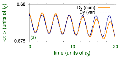
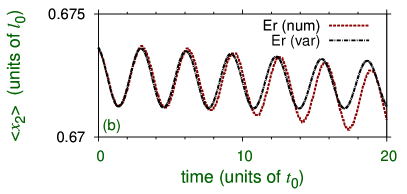
Figure 10: Numerical (num) and variational (var) time evolutions of rms size $\langle x\rangle$ of (a) ¹⁶⁴Dy and (b) ¹⁶⁸Er components in the binary soliton of figure 4 upon a small perturbation.

We investigate the dynamics of an axially-symmetric binary ¹⁶⁴Dy-¹⁶⁸Er soliton free to move along the axial $z$ direction and radially trapped by the potential $\rho^{2}/2$. A small oscillation is generated by an infinitesimal perturbation in the numerical routine. The oscillation in the radial direction is quasi sinusoidal, whereas the oscillation in the axial direction is found to be more complicated. This is due to the presence of the harmonic trap in the radial direction. In figures 10 (a) and (b), to show the radial oscillation of the two components of the binary soliton we plot the time evolution of the rms size $\langle x\rangle$ of the two components $-$ ¹⁶⁴Dy and ¹⁶⁸Er, respectively. The same oscillations generated from the variational equations (12) $-$ (15) are also shown in these figures. Considering the complicated dynamics the agreement between the two results is quite satisfactory.

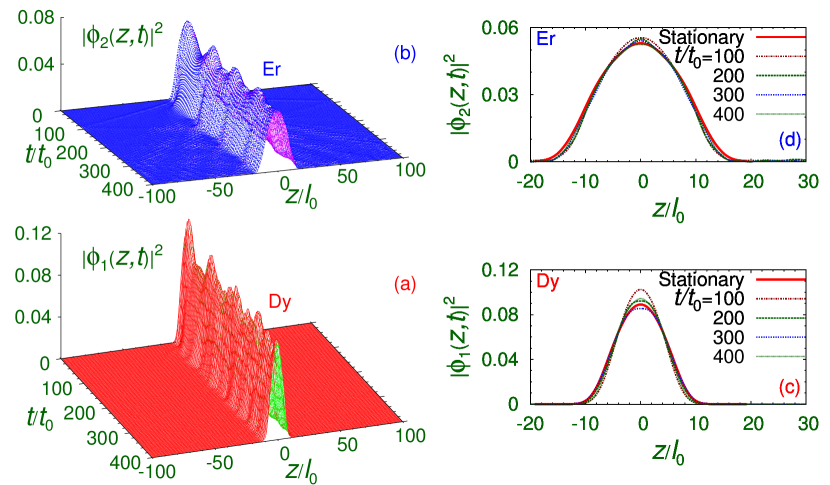
Figure 11: Integrated 1D density $|\phi_{i}(z;t)|^{2}=\int dx\int dy|\phi_{i}({\bf r},t)|^{2}$ of (a) Dy and (b) Er atoms during real-time propagation when the axial trap of angular frequency $\omega_{z}=2\pi\times 3$ Hz on a quasi-1D axially-symmetric binary dipolar BEC of 1000 Dy and 5000 Er atoms is removed linearly for $20>t/t_{0}>0$ and the resultant soliton is propagated for $t/t_{0}>20$. The profiles of the 1D density of (c) Dy and (d) Er atoms at times $t/t_{0}=100,200,300$ and 400 during real-time propagation compared with the stationary 1D density of the binary soliton obtained from imaginary-time propagation (Stationary). Parameters used in simulation: $a_{dd}($Dy$)=132.7a_{0};a_{dd}($Er$)=66.6a_{0};a_{dd}($Dy-Er$)=94.0a_{0};a($Dy$)=120a_{0};a($Er$)=60a_{0};a($Dy-Er$)=70a_{0};\omega_{\rho}=2\pi\times 61$ Hz.

As the dipolar solitons are robust and stable, they can be prepared and studied experimentally relatively easily as compared to nondipolar solitons. To obtain a quasi-1D dipolar binary soliton free to move along axial $z$ direction and bound by the harmonic trap $\rho^{2}/2$ in the $x-y$ plane, first, we prepare a quasi-1D binary dipolar BEC bound under an weak axial trap: $V({\bf r})=(\rho^{2}+\lambda^{2}z^{2})/2,\lambda=0.05$, corresponding to radial and axial traps with angular frequencies $\omega_{\rho}=2\pi\times 61$ Hz and $\omega_{z}\approx 2\pi\times 3$ Hz. Then we slowly and linearly remove the axial trap in 20 units of dimensionless time $t/t_{0}$, when the bound binary dipolar BEC turns to a binary dipolar BEC soliton. To illustrate the viability of this scheme we prepare the axially-symmetric binary dipolar BEC wave functions in imaginary-time propagation of Eqs. (7) and (8) with $\nu_{1}=\gamma_{1}=\nu_{2}=\gamma_{2}=1$ and $\lambda_{1}=\lambda_{2}=0.05$. The dipolar binary BEC wave functions obtained in imaginary-time simulation is then used in the real-time routine to study the dynamics of the preparation of the dipolar binary soliton. During real-time propagation, from $t/t_{0}$ = 0 to 20 the axial trap $\lambda^{2}z^{2}/2$ is gradually (linearly) reduced to zero, so that for $t/t_{0}>20$ the axially free quasi-1D binary dipolar soliton emerges. Then we continue the real-time propagation for a large interval of time and establish a stable binary soliton at large times. The result of the simulation is presented in figure 11, where we plot the integrated 1D densities $|\phi_{i}(z,t)|^{2}=\int dx\int dy|\phi({\bf r},t)|^{2}$ during real-time propagation. We further confirm that the profiles of the binary dipolar soliton oscillated a little during real-time propagation around the stationary soliton profiles obtained from imaginary-time propagation. To this end, we show in figures 11 (c) and (d) the 1D density of Dy and Er atoms at times $t/t_{0}=100,200,300,$ and 400 together with the converged stationary imaginary-time profiles. The stable and robust peaks of the component solitons confirm the solitonic nature of the binary BEC. In this fashion all the binary solitons could be realized in laboratory, by including a weak trap along the free propagation direction(s) and eventually realeasing these traps slowly. A nondipolar BEC soliton stabilized by contact attraction alone cannot be prepared in this fashion.

4 Summary and Discussion

Using variational approximation and numerical solution of a set of coupled 3D mean-field GP equations, we demonstrate the existence of a dipolar binary ¹⁶⁴Dy-¹⁶⁸Er soliton stabilized by inter- and intraspecies dipolar interactions in the presence of repulsive inter- and intraspecies contact interactions. The domain of stability of the binary soliton is highlighted in stability phase diagrams of number of ¹⁶⁴Dy and ¹⁶⁸Er atoms and interspecies scattering length $a_{12}$ for fixed dipolar interactions and intraspecies contact interactions. We considered distinct spatial shapes of the two components of the binary dipolar soliton, e.g., (a) both with quasi-1D profile along the polarization $z$ direction, (b) both with quasi-2D profile in the $y-z$ plane, (c) one component with quasi-1D profile along the $z$ direction and the other with quasi-2D profile in the $y-z$ plane, (d) one component with quasi-2D profile in the $y-z$ plane and the other with quasi-2D profile in the $x-z$ plane, etc. Results of variational approximation and numerical solution for the statics (sizes and chemical potentials) and dynamics (breathing oscillation) of the binary ¹⁶⁴Dy-¹⁶⁸Er soliton with both components having axially-symmetric quasi-1D profile are found to be in satisfactory agreement with each other.

The solitons considered in this work are stabilized by long-range dipolar attraction and short-range contact repulsion. The repulsion in the dipolar interaction is equilibrated by a harmonic trap. Hence unlike normal BEC solitons stabilized by short-range contact attraction alone, the present dipolar BEC solitons will be more immune to collapse due to short-range repulsion and can easily accommodate 10000 atoms of the binary ¹⁶⁴Dy-¹⁶⁸Er mixture as can be seen from Figs. 2 and 3. A possible way of preparing these binary dipolar solitons is suggested. As these solitons are robust and stable one can first prepare the binary dipolar BECs with weak traps along the mobile directions. Then these weak traps are to be removed slowly, when the binary BECs will turn to binary solitons. The viability of this approach is demonstrated by real-time simulation. Hence these solitons could be of great experimental interest. With the present experimental techniques, such binary dipolar BECs can be observed and the conclusions of the present study verified.

References

References

• [1] Strecker K E, Partridge G B, Truscott A G and Hulet R G 2002 Nature 417 150
• [2] Khaykovich L, Schreck F, Ferrari G, Bourdel T, Cubizolles J, Carr L D, Castin Y and Salomon C 2002 Science 256 1290
• [3] Cornish S L, Thompson S T and Wieman C E 2006 Phys. Rev. Lett.96 170401
• [4] Perez-Garcia V M, Michinel H and Herrero H 1998 Phys. Rev.A 57 3837
• [5] Lu M, Youn S H and Lev B L 2010 Phys. Rev. Lett.104 063001 McClelland J J and Hanssen J L 2006 Phys. Rev. Lett.96 143005 Youn S H, Lu M W, Ray U and Lev B L 2010 Phys. Rev.A 82 043425
• [6] Lu M, Burdick N Q, Youn S H and Lev B L 2011 Phys. Rev. Lett. 107 190401
• [7] Aikawa K, Frisch A, Mark M, Baier S, Rietzler A, Grimm R and Ferlaino F 2012 Phys. Rev. Lett. 108 210401
• [8] Lahaye T et al. 2009 Rep. Prog. Phys. 72 126401
• [9] Lahaye T et al. 2007 Nature 448 672
• [10] Stuhler J et al. 2005 Phys. Rev. Lett.95 150406
• [11] Goral K, Rzazewski K and Pfau T 2000 Phys. Rev.A 61 051601
• [12] Koch T et al. 2008 Nature Phys. 4 218 Griesmaier A et al. 2006 Phys. Rev. Lett.97 250402
• [13] Deiglmayr J, Grochola A, Repp M, Mörtlbauer K, Glück C, Lange J, Dulieu O, Wester R and Weidemüller M 2008 Phys. Rev. Lett. 101 133004 de Miranda M H G et al. 2011 Nature Phys. 7 502
• [14] Young-S L E, Muruganandam P and adhikari S K 2011 J. Phys. B: At. Mol. Opt. Phys.44 101001
• [15] Pedri P and Santos L 2005 Phys. Rev. Lett.95 200404 (2005) Tikhonenkov I, Malomed B A and Vardi A 2008 Phys. Rev.A 78 043614 Tikhonenkov I, Malomed B A and Vardi A 2008 Phys. Rev. Lett.100 090406 Köberle P, Zajec D, Wunner G and Malomed B A 2012 Phys. Rev.A 85 023630
• [16] Adhikari S K and Muruganandam P 2012 Phys. Lett. A 376 2200
• [17] Adhikari S K and Muruganandam P 2012 J. Phys. B: At. Mol. Opt. Phys.45 045301
• [18] Wilson R M, Ticknor C, Bohn J L and Timmermans E 2012 Phys. Rev.A 86 033606 Saito H, Kawaguchi Y and Ueda M 2009 Phys. Rev. Lett.102 230403
• [19] Young-S L E and Adhikari S K 2012 Phys. Rev.A 86 063611
• [20] Lamporesi G et al. 2010 Phys. Rev. Lett.104 153202
• [21] Young-S L E, Salasnich L and Adhikari S K 2010 Phys. Rev.A 82 053601
• [22] Yi S and You L 2001 Phys. Rev.A 63 053607
• [23] Goral K and Santos L 2002 Phys. Rev.A. 66 023613
• [24] Perez-Garcia V M, Michinel H, Cirac J I, Lewenstein M and Zoller P 1997 Phys. Rev.A 56 1424
• [25] Muruganandam P and Adhikari S K 2009 Comput. Phys. Commun. 180 1888 Vudragovic D, Vidanovic I, Balaz A, Muruganandam P and Adhikari S K 2012 Comput. Phys. Commun. 183 2021
• [26] Inouye S et al. 1998 Nature 392 151
• [27] Blatt S, Nicholson T L, Bloom B J, Williams J R, Thomsen J W, Julienne P S and Ye J 2011 Phys. Rev. Lett.107 073202