On the numerical stability of the least-squares method for the planar scattering by obstacles

Abstract

The scattering of waves by obstacles in a 2D setting is considered, in particular the computation of the scattered field via the collocation or the least-squares methods. In the case of multiple scattering by smooth obstacles, we prove that the scattered field can be uniformly approximated by sums of multipoles. For a unique obstacle, the choice of the number of points and their positions for the estimation of the error on the border of the scatterer is studied, showing the benefit of using a non-uniform distribution of points dependent on the scatterer and the approximation scheme. In general, using a denser discretization near the singularities of the scattered field does not improve the stability of the method. The analysis can also be used to estimate the discretization size needed to ensure stability given a density of points and an approximation scheme, e.g. in the case of multiple scatterers.

1 Introduction

This article is concerned with the least-squares method for the Helmholtz equation [1, 2]. Like other methods such as the Boundary Element Method, the Variational Theory of Complex Rays [3], or the Ultra-weak variational Formulation [4], it solves the Helmholtz equation by using an approximation scheme for the solutions to the equation (plane waves, generalized harmonic polynomials, etc.). These methods differ by the way they match the solution to the boundary conditions and ensure the continuity between the elements. With the least-squares method, the boundary conditions and the continuity between the subdomains are enforced via the minimization of a $L_{2}$-norm, allowing a simple implementation of the method.

In the particular case of the scattering of an incident wave $u_{i}$ by obstacles $S$ in the plane with Dirichlet boundary conditions, the scattered field is solution to:

$$\left\{\begin{array}[]{l}\Delta u_{s}+k^{2}u_{s}=0\\ u_{s}=-u_{i}\mbox{ on }\partial S\\ \lim_{r\rightarrow\infty}\sqrt{r}\left(\frac{\partial u_{s}}{\partial r}-iku_{s}\right)=0\end{array}\right.$$ (1)

The resolution of this problem via the least-squares method was studied, among others, by Stojek [2], and Barnett and Betcke [5]. The domain of propagation was partitioned in bounded subdomains where Fourier-Bessel functions, or fractional Fourier-Bessel functions in the case of a scatterer with corners, were used for the approximation, and an unbounded domain. In this domain, Stojek used Hankel functions to enforce the Sommerfeld radiation condition, while Barnett and Betcke used the Method of Fundamental Solutions. We restrict ourselves to the somewhat simpler case, but equally interesting, of the scattering by smooth obstacles, that, as will be shown in this article, allows the approximation of the solutions on the entire unbounded domain of propagation using a single set of functions.

In the case of a unique scatterer, this approximation is the basis of the so-called Rayleigh methods[6], where the scattered field is approximated by sums of multipoles

$$u_{s}\approx u_{N}=\sum_{n=-N_{h}}^{N_{h}}\alpha_{n}H_{n}(kr)e^{in\theta}$$ (2)

where $(r,\theta)$ are the polar coordinates. The collocation method, or Point Matching Method, estimates the $2N_{h}+1$ coefficients by fitting the boundary conditions on $2N_{h}+1$ points on the border of the scatterer. While simple to implement, this method is usually numerically unstable as the matrix to be inverted is likely to be ill-conditioned. The coefficients can also be estimated by minimizing the $L_{2}$ error on the boundary, where the error is approximated by numerical quadrature. This can be considered as a particular case of the least-squares methods cited above, where the approximation is done on the entire domain like in [7]. However, in the case of scattering by an obstacle, the domain is multiply-connected and unbounded. As is usually observed in this particular case [8, 9], but also in the general case [2, 1, 5], the matrices involved in the computation have the tendency to be ill-conditioned.

In this article, we investigate the effect of the choice of the quadrature points on the numerical stability of the least-squares method in the particular case of the scattering by an obstacle. The quadrature used to estimate the error is generally either left unspecified [1, 2, 10, 11], or uses general purpose schemes (Chebyshev nodes in [12] or Clenshaw-Curtis rule in [5]). However, as was shown in [8] for the collocation method, the choice of the quadrature point is critical for the stability of the numerical methods, and depends on the shape of the scatterer. This has direct implications on the efficiency of the computational methods, as choosing the appropriate quadrature rule allows to use fewer points, making the matrices involved in the computation smaller.

This work is a first step towards a more general study of the effect of the quadrature scheme on the numerical stability of least-squares methods (i.e. with other approximations schemes such as plane waves, Fourier-Bessel functions, fractional Fourier-Bessel functions, and with several subdomains), but is also interesting in itself as it gives a stable numerical scheme for the scattering by an obstacle, a long standing problem in electromagnetics and acoustics[6, 9, 8, 13].

In section 2, we prove an approximation result for the scattering of waves by smooth obstacles: given a set of $L$ smooth scatterers $S_{l}$, the scattered field $u_{s}$, solution to (1), can be uniformly approximated by a sequence of sums of multipoles

$$u^{N}=\sum_{l=1}^{L}\sum_{n\in\mathbf{Z}}\beta_{nl}^{N}H_{n}(kr_{l})e^{in\theta_{l}}$$ (3)

where $(r_{l},\theta_{l})$ are the polar coordinates with respect to a center $O_{l}$, with at least one such center in each scatterer, and a finite number of coefficients $\beta_{nl}^{N}$ are nonzero. In the third section of the paper, the stability of the least-squares method is investigated in the light of a recent result by Cohen et al. [14] on least-squares approximations, and numerical results are given for the scattering by an ellipse and a square, demonstrating the importance of the choice of the quadrature points. In particular, it is shown that in some cases, using a denser discretization near the singularities makes the stability harder to achieve than using a uniform density or even a denser discretization away from the singularities. Finally, the application to the scattering of a plane wave by two arbitrary shaped scatterers is given.

2 Approximation of the scattered field

We here show that the field scattered by smooth obstacles can be uniformly approximated by sums of multipoles. This is an application of the Vekua theory [15, 16], a theory of elliptic PDEs allowing the construction of operators mapping holomorphic functions to solutions of a given PDE, as long as the coefficients of the PDE are analytic. This is obviously true for the Helmholtz equation, for which the operator mapping holomorphic (or equivalently harmonic) functions to solutions to the Helmholtz equation and its inverse are explicitly known. These operators being continuous, approximation results available for holomorphic functions can be translated to similar results for solutions to the Helmholtz equation. For instance, in a star-shaped domain, solutions to the Helmholtz equation can be approximated by sums of Fourier-Bessel functions $J_{n}(kr)e^{in\theta}$, that are the images of the harmonic polynomials used to approximate harmonic functions. More details on the Vekua operators and on the approximation of solutions to the Helmholtz equation in convex domains can be found in the articles by Moiola et al. [17, 18].

Our setting is as follows: scatterers are contained in the disk of radius $R_{1}$, and $\Omega$ is the closed domain delimited by the circle of radius $R_{2}>R_{1}$ and the scatterers, see figure 1.

Theorem 1.

Let $S$ be a set of scatterers in the plane, and $u_{s}$ the scattered field. If $u_{s}$ can be analytically continued in a open domain containing $\mathbf{R}^{2}-S$, then $u_{s}$ can be uniformly approximated, in $\mathbf{R}^{2}-S$ as well as on the boundaries of $S$, by a sequence $u^{N}$ of sums of Fourier-Hankel functions

$$u^{N}=\sum_{l=1}^{L}\sum_{n\in\mathbf{Z}}\beta_{nl}^{N}H_{n}(kr_{l})e^{in\theta_{l}}$$ (4)

where $(r_{l},\theta_{l})$ are the polar coordinates associated to the centers $O_{l}$, with at least such a center in each scatterer, and finitely many coefficients $\beta_{nl}^{N}$ are nonzero for a given $N$.

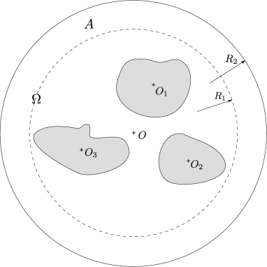
Figure 1: Domain on which the Vekua theory is applied

Proof.

The proof is divided in three main parts:

• the approximation of the scattered field in $\Omega$ by sums of first-kind Fourier-Bessel functions and outgoing Fourier-Hankel functions,

• the use of the Sommerfeld radiation condition to reduce this approximation to sums of outgoing Hankel functions,

• the extension of this approximation outside of $\Omega$.

General representation in $\Omega$

For a closed multiply-connected domain $\Omega$ and the Helmholtz equation, Vekua proved (see Ref.[15] page 109) that if a solution $u$ can be analytically continued in an open domain containing $\Omega$, then $u$ can be uniformly approximated by a sequence of finite sums of Fourier-Bessel functions of the first and second kind

$$J_{n}(kr)e^{in\theta},Y_{n}(k_{l}r)e^{in\theta_{l}}$$

where $(r,\theta)$ are the polar coordinates with respect to the origin $O$, and $(r_{l},\theta_{l})$ with respect to $O_{l}$, with at least a point $O_{l}$ arbitrarily chosen in the $l$-th simply connected component of $\mathbf{R}^{2}-\Omega$. As we can uniformly approximate the functions $J_{n}(kr_{l})e^{in\theta_{l}}$ by sums of $J_{m}(kr)e^{im\theta}$ (Graf theorem), we can equivalently approximate $u$ by sums of first kind Fourier-Bessel functions and outgoing Fourier-Hankel functions:

$$J_{n}(kr)e^{in\theta},H_{n}(k_{l}r)e^{in\theta_{l}}$$

We apply this theorem in $\Omega$. We have thus that $u^{N}$, defined as

$$u^{N}=\sum_{n\in\mathbf{Z}}\alpha_{n}^{N}J_{n}(kr)e^{in\theta}+\sum_{l=1}^{L}\sum_{n\in\mathbf{Z}}\beta_{nl}^{N}H_{n}(kr_{l})e^{in\theta_{l}}$$ (5)

where only a finite number of coefficients $\alpha_{n}^{N}$ and $\beta_{nl}^{N}$ are nonzero, uniformly converges to $u_{s}$ as $N\rightarrow\infty$.

Removal of the first term in (5)

In the annulus $A$ of radiuses $R_{1}$ and $R_{2}$ we can, by moving the Hankel functions to $O$ (using the Graf theorem), approximate $u_{s}$ as the limit of a sum of first-kind Bessel functions and a series of Hankel functions with coefficients functions of $N$.

$$u^{N}=\sum_{n\in\mathbf{Z}}\alpha_{n}^{N}J_{n}(kr)e^{in\theta}+\beta_{n}^{N}H_{n}(kr)e^{in\theta}$$ (6)

For $r\geq R_{1}$, $u$ can also be written as a series of Hankel functions as it satisfies the Sommerfeld radiation conditions:

$$u_{s}=\sum_{n\in\mathbf{Z}}\gamma_{n}H_{n}(kr)e^{in\theta}$$ (7)

Fitting the sequence (6) to the series (7) in the annulus $A$ will allow to show that $u_{s}$ can be approximated by Hankel functions around the scatterers.

Let $\epsilon>0$ and $R^{\prime}_{2}$ with $R_{1}<R^{\prime}_{2}<R_{2}$. Then there is a $N_{1}$ such that for $N>N_{1}$,

$$|u^{N}-u_{s}|=\left|\sum_{n\in\mathbf{Z}}\alpha_{n}^{N}J_{n}(kR^{\prime}_{2})e^{in\theta}+\beta_{n}^{N}H_{n}(kR^{\prime}_{2})e^{in\theta}-\gamma_{n}H_{n}(kR^{\prime}_{2})e^{in\theta}\right|<\epsilon$$ (8)

The coefficients of the Fourier series of $u^{N}-u_{s}$ satisfy

$$\left|\alpha^{N}_{n}J_{n}(kR^{\prime}_{2})+\beta^{N}_{n}H_{n}(kR^{\prime}_{2})-\gamma_{n}H_{n}(kR^{\prime}_{2})\right|<\epsilon$$ (9)

As the functions $u^{N}$ and their limit are analytic, we can do the same for the radial derivative. For $N>N_{2}$:

$$k\left|\alpha^{N}_{n}J_{n}^{\prime}(kR^{\prime}_{2})+\beta^{N}_{n}H_{n}^{\prime}(kR^{\prime}_{2})-\gamma_{n}H_{n}^{\prime}(kR^{\prime}_{2})\right|<k\epsilon$$ (10)

For $N>\max(N_{1},N_{2})$, we have

$$\alpha^{N}_{n}J_{n}(kR^{\prime}_{2})+\beta^{N}_{n}H_{n}(kR^{\prime}_{2})=\gamma_{n}H_{n}(kR^{\prime}_{2})+\delta_{n}$$ (11)

$$\alpha^{N}_{n}J_{n}^{\prime}(kR^{\prime}_{2})+\beta^{N}_{n}H_{n}^{\prime}(kR^{\prime}_{2})=\gamma_{n}H_{n}^{\prime}(kR^{\prime}_{2})+\delta^{\prime}_{n}$$ (12)

with $|\delta_{n}|<\epsilon$ and $|\delta^{\prime}_{n}|<\epsilon$

Solving this system for $\alpha^{N}_{n}$ (using the fact that the wronskian[19] of $J_{n}$ and $H_{n}$ is equal to $2i/(\pi kR^{\prime}_{2}$) we have

$$\alpha^{N}_{n}=\frac{2i(\delta_{n}H_{n}^{\prime}(kR^{\prime}_{2})-\delta_{n}^{\prime}H_{n}(kR^{\prime}_{2}))}{\pi kR^{\prime}_{2}},$$ (13)

and, with $C=2/\pi kR^{\prime}_{2}$

$$|\alpha^{N}_{n}|\leq C\epsilon\left(|H_{n}^{\prime}(kR^{\prime}_{2})|+|H_{n}(kR^{\prime}_{2})|\right).$$ (14)

We now uniformly bound the first term of (6) for $r\leq R^{\prime\prime}_{2}<R^{\prime}_{2}$. We have $|\sum\alpha^{N}_{n}J_{n}(kr)|\leq\sum|\alpha^{N}_{n}J_{n}(kr)|\leq C\epsilon\sum(|H_{n}^{\prime}(kR^{\prime}_{2})|+|H_{n}(kR^{\prime}_{2})|)|J_{n}(kr)|$ and

$$\sum_{n\in\mathbf{Z}}(|H_{n}^{\prime}(kR^{\prime}_{2})|+|H_{n}(kR^{\prime}_{2})|)|J_{n}(kr)|=\sum_{|n|<kR^{\prime\prime}_{2}}(|H_{n}^{\prime}(kR^{\prime}_{2})|+|H_{n}(kR^{\prime}_{2})|)|J_{n}(kr)|+\sum_{|n|\geq kR^{\prime\prime}_{2}}(|H_{n}^{\prime}(kR^{\prime}_{2})|+|H_{n}(kR^{\prime}_{2})|)|J_{n}(kR^{\prime\prime}_{2})|$$ (15)

where we used the fact that $|J_{n}|$ is increasing on $[0,n]$. This first term is a continuous function and can be uniformly bounded, and the second term is a convergent series:

$$(|H_{n}^{\prime}(kR^{\prime}_{2})|+|H_{n}(kR^{\prime}_{2})|)|J_{n}(kR^{\prime\prime}_{2})| \sim|H_{n+1}(kR^{\prime}_{2})||J_{n}(kR^{\prime\prime}_{2})|$$ (16)

$$\sim\frac{1}{\sqrt{n+1}}\left(\frac{ekR^{\prime}_{2}}{2(n+1)}\right)^{-n-1}\frac{1}{\sqrt{n}}\left(\frac{ekR^{\prime\prime}_{2}}{2n}\right)^{n}$$ (17)

$$\sim(R^{\prime\prime}_{2}/R^{\prime}_{2})^{n}/(kR^{\prime}_{2})$$ (18)

We thus have, with $C^{\prime}$ the quantity in (15),

$$\left|\sum_{n\in\mathbf{Z}}\alpha^{N}_{n}J_{n}(kr)\right|\leq\epsilon CC^{\prime}$$ (19)

The first term of (5) can be made uniformly as small as desired, and can be removed from the sequence $u^{N}$ without changing its limit for $r<R^{\prime\prime}_{2}$.

Convergence outside $\Omega$

We now have that the sequence

$$u^{N}=\sum_{l=1}^{L}\sum_{n\in\mathbf{Z}}\beta_{nm}^{N}H_{n}(kr_{l})e^{in\theta_{l}}$$ (20)

uniformly converges to $u_{s}$ outside of the obstacles and on their boundaries, for $r\leq R^{\prime\prime}_{2}$.

For $R_{1}\leq r\leq R_{2}$, we have (cf. (6)) that

$$u^{N}=\sum_{n\in\mathbf{Z}}\beta_{n}^{N}H_{n}(kr)e^{in\theta}$$ (21)

converges uniformly to

$$u_{s}=\sum_{n\in\mathbf{Z}}\gamma_{n}H_{n}(kr)e^{in\theta}.$$ (22)

On the circle of radius $R_{1}$, the error between $u_{N}$ and $u$ converges uniformly to 0. The coefficients of the Fourier transform of the error can be bounded:

$$|\beta_{n}^{N}-\gamma_{n}|<\epsilon/H_{n}(kR_{1})$$ (23)

Now, for any $r>R^{\prime}_{1}$ (with $R_{1}<R^{\prime}_{1}<R^{\prime\prime}_{2}$), we have

$$|u^{N}-u_{s}| \leq\sum_{n\in\mathbf{Z}}|\beta_{n}^{N}-\gamma_{n}||H_{n}(kr)\|$$ (24)

$$\leq\epsilon\sum_{n\in\mathbf{Z}}|H_{n}(kR^{\prime}_{1})|/|H_{n}(kR_{1})|$$ (25)

$$\leq\epsilon C$$ (26)

as the general term of the last series is equivalent to $(R^{\prime}_{1}/R_{1})^{n}$. We here used the fact that $|H_{n}|$ is a decreasing function.

The error between $u^{N}$ and $u_{s}$ can be bounded by any $\epsilon$ for any $r>R^{\prime}_{1}$. Combined with the fact that $u^{N}$ converges uniformly to $u_{s}$ for $r<R^{\prime\prime}_{2}$ outside of the obstacles and on their boundaries, $u^{N}$ converges uniformly to $u_{s}$ outside of the scatterers and on their boundaries, yielding the theorem. ∎

To conclude this section, we formulate a conjecture based on the analogy between Runge’s theorem and Theorem 1. This theorem states that an analytic function on a given open domain can be, in a compact subdomain, uniformly approximated by a sequence of rational functions, with at least a pole in each connected component of the complement of its domain of analyticity. The connection between this result for analytic functions and solutions to the Helmholtz equation is given by the Vekua theory. The conditions of Runge’s theorem can actually be weakened, as shown by Mergelyan’s theorem[20]. This theorem states that it is sufficient that the function to be approximated is holomorphic in the interior of $\Omega$ and only continuous on the boundaries of $\Omega$. In particular, singularities can be present on the boundaries, which is likely for domains with corners. It is then reasonable to formulate this conjecture:

Conjecture 1.

The uniform approximation by sum of multipoles is valid as long as the scattered field is analytic in the exterior of the obstacles, and continuous on their boundaries.

This condition is in particular satisfied for domain with corners, Dirichlet conditions and a continuous incident field. Although this conjecture is of theoretical interest, its usefulness in numerical applications is limited. Indeed, the presence of singularities on the boundary of the obstacles limits the rate of convergence of the Vekua approximations [18]. Convergence can be accelerated by the use of fractional Fourier-Bessel functions in the approximation[5], but this necessitates the partition of the exterior domain in simply connected subdomains, making multipole approximations irrelevant.

3 Stability of numerical methods

In the previous section, we proved that uniform approximation of the scattered field was possible for smooth scatterers, that is that the error between the scattered field $u_{s}$ and its best approximation $u^{N}$ of order $N$ tends uniformly to zero:

$$\|u_{s}-u^{N}\|_{\infty}\rightarrow 0.$$

We are here interested in least-squares method for the case of a unique scatterer. The uniform convergence implies local convergence in the $L_{2}$-norm (that is, on any compact domain):

$$\|u_{s}-u^{N}\|_{2,loc}\rightarrow 0.$$

In particular, it implies the convergence in the $L_{2}$ norm on the boundary $\Gamma$ of the scatterer. The following theorem, proved in [10], shows that the convergence on the boundary of the scatterer is sufficient to ensure convergence outside:

Theorem 2.

(Ramm, Gutman) If $g$ is in $L^{2}(\Gamma)$, then the solution $w$ of the Helmholtz equation with Sommerfeld radiation conditions and $w=g$ on $\Gamma$ is bounded on the exterior domain $D^{\prime}$ by

$$\|w\|\leq C\|g\|_{L^{2}(\Gamma)}$$ (27)

where $\|w\|=\|w\|_{H^{m}_{loc}(D^{\prime})}+\|w\|_{L^{2}(D^{\prime},(1+|x|)^{-\gamma})}$, with $H^{m}$ with $m>0$ is the Sobolev space and the $L^{2}$ norm is weighted by $(1+|x|)^{-\gamma}$ with $\gamma>1$.

However, this does not guarantee that practical computation of the scattered field will always converge to the true solution when increasing the order of approximation. To this end, the estimation of the coefficients of this finite approximation has to be stable, that is that the error (e.g. on the boundary $\Gamma$) between this estimated field $\tilde{u}^{N}$ and the actual field is of the same order as the best approximation error:

$$\|u_{s}-\tilde{u}^{N}\|_{2,\Gamma}\approx\|u_{s}-u^{N}\|_{2,\Gamma}.$$

In this section, we analyze the numerical stability of the computation of the scattered field using the multipole approximation and the collocation or least-squares methods. Through numerical evaluation of the stability, we aim to show that the density of points used on the border of the scatterers is critical for the stability. The tool used for the analysis can also be used to estimate, given an approximation scheme and a sampling density (e.g. multipole approximation with uniform density on the border), the number of samples needed to ensure stability.

With the least-squares methods, the scattered field is estimated as follows: given an order of approximation $N_{h}$ (i.e. $m=2N_{h}+1$ Fourier-Hankel functions) and a number $N_{s}$ of points on the boundary of the scatterer, the coefficients of the multipole approximation are estimated by matching the incoming field $u_{i}$ and the multipole approximation on the sampling points in the least-squares sense:

$$\tilde{\mathbf{a}}=\operatorname*{arg\,min}_{\mathbf{a}}\|\mathbf{u}+\mathbf{H}\mathbf{a}\|_{2}$$ (28)

where $\tilde{\mathbf{a}}=(\alpha_{-N_{h}},\ldots,\alpha_{N_{h}})$ is the vector containing the estimated coefficients, $\mathbf{u}$ the vector of the values of $u_{i}$ sampled on the boundary, and $\mathbf{H}$ the $N_{s}\times 2N_{h}+1$ matrix with terms

$$H_{mn}=H_{n}(kr_{m})e^{in\theta_{m}}$$

where $n\in\{-N_{h},\ldots N_{h}\}$ and $(r_{m},\theta_{m})$ are the polar coordinates of the $N_{s}$ points on the boundary. Note that the Sommerfeld radiation condition does not need to be considered in the minimization problem as it is enforced through the choice of the approximation spaces. The estimated scattered field is then given by

$$\tilde{u}_{s}=\sum_{|n|\leq N_{h}}\alpha_{n}H_{n}(kr)e^{in\theta}.$$

The collocation method, or point matching method, is a particular case of the least-squares method, obtained when $N_{s}=2N_{h}+1$. In this case, the matrix $\mathbf{H}$ is square, and the coefficients are found by matching the values of the samples in an exact way.

With these methods, estimation of the scattered field is essentially reduced to the interpolation of the incident field on the boundary of the scatterer using a finite number of functions (the traces of the multipoles on the boundary) from a finite number of samples. However, it is well known that even in basic cases, interpolation of a function from a finite number of samples can be unstable (cf. Runge phenomenon), even when the data is perfectly known on the sampling points.

3.1 Stability of least-squares estimation

To analyze the stability of these methods in function of $N_{h}$, $N_{s}$ and the density of samples, we use results by Cohen et al [14]. These results allow the estimation of the number of measurements ensuring stability, knowing the density probability measure used to draw the points on the border, as well as the desired order of approximation. While the sampling points are not generally chosen randomly, and the values obtained are somewhat pessimistic, these results will help to evaluate the stability of sampling densities.

The setting is as follows. The functions to be estimated, defined on a space $X$, are known to be approximated by elements of spaces $V_{m}$ of dimension $m$, and the best approximation error of $u$ by an element of $V_{m}$ is denoted by $\sigma_{m}(u)$. The estimation $\tilde{u}$ is obtained by the least-squares method using $n$ samples, drawn from the space $X$ using the probability density $\nu$, and truncated so that its absolute value is not larger than $M=\max_{x\in X}|u(x)|$.

To evaluate the stability of this least-square estimation we compute the quantity

$$K(m)=\max_{x\in X}\sum_{j=1}^{m}|L_{j}(x)|^{2}$$ (29)

where $(L_{j})_{j}$ is a basis of the space $V_{m}$, orthogonal with respect to the probability density $\nu$:

$$\int_{X}L_{j}^{\star}L_{k}d\nu=\delta_{j,k}$$ (30)

The value of $K(m)$ is then linked to the number of measurements $n$ by the following theorem:

Theorem 3.

(Cohen, Davenport, Leviatan) Let $r>0$ be arbitrary but fixed and let $\kappa:=\frac{1-\log 2}{2+2r}$. If $m$ is such that

$$K(m)\leq\kappa\frac{n}{\log n}$$

then, the expectation of the reconstruction error is bounded:

$$E(\|u-\tilde{u}\|^{2})\leq(1+\epsilon(n))\sigma_{m}(u)^{2}+8M^{2}n^{-r},$$

where $\epsilon(n):=\frac{4\kappa}{\log n}\to 0$ as $n\to+\infty$.

In our case, the space $X$ is the border of the scatterer, and the spaces $V_{m}$ are generated by finite families of multipoles. The orthogonal basis $(L_{j})_{j}$ can be estimated by orthogonalizing a family of multipoles, using the Gram-Schmidt algorithm and numerical quadrature (e.g. Monte-Carlo integration using the probability density $\nu$).

Numerical results are now given for the scattering by an ellipse, a square, and two ovals. The code needed to reproduce the figures, as well as similar results for others scatterers are available online [21].

3.2 Scattering by an ellipse

We first estimate $K(m)$ for the case of the ellipse centered at the origin. The values of $K(m)$ for $m\in\{10,20,30,40,50\}$ and $k=6$ as a function of the eccentricity $e$ of the ellipse are given on figure 2, for the uniform density and the density suggested by Kleev and Manenkov[8] . This density (denoted by KM density in the rest of the paper) is based on a conformal mapping between the unit disk and the scatterer. The computation of this density is outlined in the appendix.

For the uniform density, the value of $K(m)$ increases with the eccentricity, meaning that more and more points are needed for a fixed number of coefficients. $K(m)$ remains nearly constant for the KM density. It is clear that this density needs less samples to ensure the stability of the interpolation. However, in contrast to the claim of Kleev and Manenkov that the density depends on the singularities of the scattered field, these results shows that the density does not depend on these singularities, but on the singularities of the functions used for the interpolation. Indeed, as the eccentricity of the ellipse increases, the singularities, located at the focal points of the ellipse, approaches the extremities of the major axis, while the sampling becomes denser near the extremities of the minor axis, i.e. near the singularities of the functions used to approximate the scattered field (see figure 3).

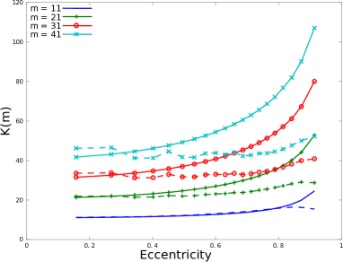
Figure 2: Estimated $K(m)$ for the ellipse at $k=6$ in functions of the eccentricity, for the uniform density (solid) and the density obtained by Kleev (dashed)

Figure 3: Samplings on the ellipse, with eccentricity $e=0.95$. Left: uniform density, center: KM density, right: uniform density on the circle mapped to the ellipse

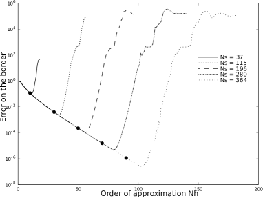
Figure 4: $L_{2}$-Error on the boundary for the scattering of a plane wave by an ellipse, with eccentricity $e=0.8$ for several numbers of samples, and varying orders of approximation. For each number of samples, the order $N_{h}$ such that $N_{s}\approx K(2N_{h}+1)$ is highlighted.

On figure 4, we plot, for some fixed numbers $N_{s}$ of samples on the boundary, the $L_{2}$ approximation error on the border in function of the approximation order $N_{h}$ for $e=0.8$ and $k=6$. This error on the border is an indicator of the quality of the estimation of the scattered field. Indeed, as Theorem 2 shows, the error outside of the scatterer can be bounded by the error on the border. The orders for which $N_{s}=K(2N_{h}+1)$ are indicated. As the approximation errors for these choices of parameters are close the optimal errors, we suggest to use $K(2N_{h}+1)$ samples when using an order of approximation of $N_{h}$.

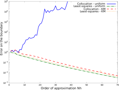
Figure 5: $L_{2}$-error on the boundary for the scattering of a plane wave by an ellipse with eccentricities $e=0.86$ and varying approximation orders. The error is given for the collocation and the least-squares methods, with uniform and KM densities. For the least-squares, the number of samples is given by $K(m)$.

On figure 5, the $L_{2}$ error between the estimated scattered field and the incident field on the border is plotted for the result of the collocation and the least-squares method, with the uniform and the KM densities, in function of the approximation order for an eccentricity $e=0.86$ and $k=10$. For the least-squares estimation, we use $K(m)$ samples. The collocation with uniform density fails as the error increases with the approximation order. Using the KM density makes the collocation method stable. For the uniform density, using $K(m)$ samples yields a stable estimation. For the KM density, using $K(M)$ samples slightly improves the results.

We now estimate $K(m)$ when the scattered field is approximated using Mathieu functions, which give separable solutions to the Helmholtz equation in elliptic coordinates [22]. This method is used in [23] to compute the scattering by multiple ellipses. We test here two densities, the uniform density, and the density obtained by stretching the uniform density on a circle (see Fig. 3). Note that the Mathieu functions are orthogonal for this second density, and that their values on the ellipse do not depend on the wavenumber. We find here that in this case, a better stability is obtained by using the stretched density, that is when using more samples near the large axis. This is coherent with the observations above as in this case, the singularities of the functions (products of Mathieu functions in elliptical coordinates) are at the focal points of the ellipse, near the end of the major axis.

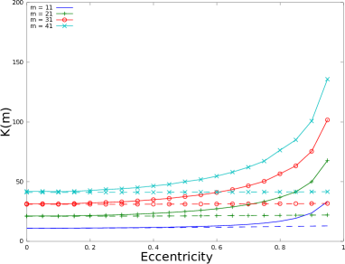
Figure 6: Estimated $K(m)$ for the ellipse in functions of the eccentricity, using Mathieu functions, for the uniform density (solid) and the uniform density on the circle mapped to the ellipse (dashed)

3.3 Scattering by a square

We now give results for the case of the unit square. We test here three densities (see figure 7):

• the uniform density,

• the KM density,

• the density $1/4\pi\sqrt{1-\min(x,y)^{2}}$.

The last density (called Chebyshev density in the rest of the paper), is similar to the sampling given by the Chebyshev nodes, used in the Clenshaw-Curtis quadrature rule. The estimation of $K(m)$ for these three densities is plotted on figure 8. Although the singularities of the scattered field are localized at the corners of the square, using a denser discretization near those corners is actually harmful to the stability of the least-squares method. Surprisingly, using more samples near the center of the edges of the square, i.e. far from the singularities, yields a $K(m)$ slightly larger than $m$, its lower bound.

The $L_{2}$ error on the border for a fixed number of samples and the three densities is plotted on figure 9 as a function of the order of approximation. Like above, the order for which $K(2N_{h}+1)\approx N_{s}$ is indicated. The KM density is stable for any approximation order, in particular for the collocation case. The uniform density can yield a slightly lower error, but is not always stable. Using more points near the corners does not allow to use a large order of approximation, and gives the largest error.

Figure 7: Samplings on the square

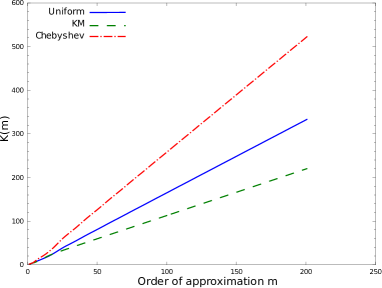
Figure 8: Estimated $K(m)$ for the square at $k=6$ for the uniform, KM and Chebyshev densities.

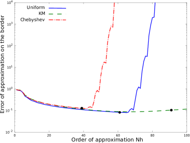
Figure 9: $L_{2}$-Error on the boundary for the scattering of a plane wave by a square for the three densities on the border and varying orders of approximation, $k=6$. For each density, the order $N_{h}$ such that $N_{s}\approx K(2N_{h}+1)$ is highlighted.

3.4 Scattering by two ovals

Our final numerical experiments deals with the scattering by two Booth ovals, defined in polar coordinates by

$$r(\theta)=1+\cos(2\theta)/a.$$

As indicated by Theorem 1, the scattered field can be approximated by two families of multipoles on the entire domain of propagation. The centers of the multipoles are chosen at the centers of the ovals (with parameters $a=2$ and $a=3$), and their borders are sampled by using a uniform sampling of the angle $\theta$, plotted on figure 10. To ensure the stability of the least-squares method, we compute $K(m)$ for the two ovals separately. With $N_{h}=65$, i.e. $m=131$, we find $K(m)=328$ for $a=2$ and $K(m)=233$ for $a=3$.

The scattered field for a incident plane wave (incoming at an angle 0.3 from the x-axis) is pictured on figure 11. The total number of degrees of freedom is 262, and 561 samples are used. Although the values of $K(m)$ are computed for the two ovals separately, using these values in the case of multiple scattering yields a stable estimation of the scattered field. This is expected, as the instabilities are mostly caused by the high order Hankel functions, which are decaying rapidly. The influence of such a function associated to a scattered on the other scatterer is thus negligible. For comparison, the result of the collocation method (i.e. using 131 samples on each scatterer) is also given.

Figure 10: Samplings on the ovals

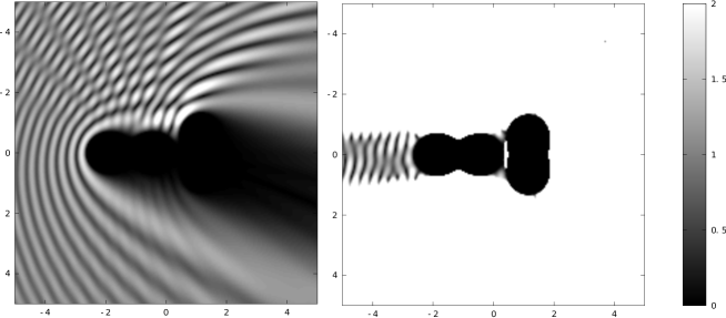
Figure 11: Scattering of a plane wave by two ovals (absolute value). Left: least-squares method. Right: collocation (thresholded at 2).

4 Conclusion

The computation of the acoustical field scattered by obstacles was considered, in particular the numerical stability of the least-squares method. We proved that the field scattered by smooth obstacles can be uniformly approximated by sums of multipoles, and that the choice of the centers of the multipoles is only limited by the constraint that at least one center is chosen in each scatterer.

We also investigated the stability of the least-squares method based on multipole approximations. This stability depends on the set of functions used to approximate the scattered field, and on the density of samples used on the boundary of the scatterer. In particular, it does not depends on the location of the singularities of the functions to be approximated. Using more points near these singularities can even be detrimental to the stability. We showed that a simple numerical computation can yield, given a set of functions and a density of samples, an estimate of the number of samples necessary to ensure stability of the least-squares method, and that it can be also used in the case of multiple scatterers. In the case of multipole approximations, the densities suggested by Kleev and Manenkov are close to the optimum.

On a more general level, we showed that in the context of least-squares or collocation methods, the approximation scheme and the quadrature rule have to be chosen conjointly.

5 Acknowledgments

The author is supported by the Austrian Science Fund (FWF) START-project FLAME (Frames and Linear Operators for Acoustical Modeling and Parameter Estimation; Y 551-N13), and thanks Vincent Pagneux and Alexandre Leblanc for fruitful discussions.

Appendix A Determination of the KM points

The densities suggested by Kleev and Manenkov are obtained by a mapping the exterior of the unit disk to the image of the scatterer by inversion. The KM points are the images of a uniform sampling of the disk by this mapping. Note that this is equivalent to a mapping from the interior of the unit disk to the scatterer with the origin as fixed point.

A.1 Case of the ellipse

A conformal mapping from the unit disk to the ellipse of major semi-axis $a$ and minor semi-axis 1 is given by (see [24])

$$f(z)=\sqrt{a^{2}-1}\sin\left(\frac{\pi}{2K(k)}\int_{0}^{z/\sqrt{k}}\frac{dt}{\sqrt{(1-t^{2})(1-k^{2}t^{2})}}\right)$$

where $K$ is the complete elliptic integral of the first kind. The parameter $k$ is found as the solution of

$$\frac{K(k^{\prime})}{K(k)}=\frac{2}{\pi}\mathrm{asinh}\left(\frac{2a}{a^{2}-1}\right)\mbox{ and }k^{\prime}=\sqrt{1-k^{2}}.$$

The KM points are then simply the images of $e^{i2\pi n/N}$ by $f$.

A.2 Case of the square

A conformal mapping from the unit disk to the square is given by the Schwartz-Christoffel mapping [25] $f$, with

$$f^{\prime}(z)=c\prod_{n=1}^{4}\left(1-\frac{z}{z_{k}}\right)^{\alpha_{k}-1}$$

where $z_{k}$ are the inverse images of the vertices and $\pi\alpha_{k}$ the angles of the square. For symmetry reason, we choose $z_{1}=1$, $z_{2}=i$, $z_{2}=-1$, $z_{2}=-i$. The $\alpha_{k}$ are equal to $1/2$. The map

$$f(z)=\int_{0}^{z}\frac{1}{\sqrt{1-z^{\prime 4}}}dz^{\prime}$$

thus maps the unit disk to a square.

References

- Monk and Wang [1999] P. Monk, D.-Q. Wang, A least-squares method for the Helmholtz equation, Computer Methods in Applied Mechanics and Engineering 175 (1999) 121 – 136.
- Stojek [1998] M. Stojek, Least-squares Trefftz-type elements for the Helmholtz equation, International Journal for Numerical Methods in Engineering 41 (1998) 831–849.
- Ladevèze et al. [2001] P. Ladevèze, L. Arnaud, P. Rouch, C. Blanzé, The variational theory of complex rays for the calculation of medium-frequency vibrations, Engineering Computations 18 (2001) 193–214.
- Cessenat and Despres [1998] O. Cessenat, B. Despres, Application of an ultra weak variational formulation of elliptic PDEs to the two-dimensional Helmholtz problem, SIAM Journal on Numerical Analysis 35 (1998) 255–299.
- Barnett and Betcke [2010] A. H. Barnett, T. Betcke, An exponentially convergent nonpolynomial finite element method for time-harmonic scattering from polygons, SIAM J. Sci. Comput. 32 (2010) 1417–1441.
- Millar [1973] R. F. Millar, The Rayleigh hypothesis and a related least-squares solution to scattering problems for periodic surfaces and other scatterers, Radio Science 8 (1973) 785–796.
- Eisenstat [1974] S. Eisenstat, On the rate of convergence of the Bergman–Vekua method for the numerical solution of elliptic boundary value problems, SIAM Journal on Numerical Analysis 11 (1974) 654–680.
- Kleev and Manenkov [1989] A. Kleev, A. Manenkov, The convergence of point-matching techniques, Antennas and Propagation, IEEE Transactions on 37 (1989) 50–54.
- Semenova and Wu [2004] T. Semenova, S. F. Wu, The Helmholtz equation least-squares method and Rayleigh hypothesis in near-field acoustical holography, The Journal of the Acoustical Society of America 115 (2004) 1632–1640.
- Ramm and Gutman [2008] A. G. Ramm, S. Gutman, Modified Rayleigh conjecture method and its applications, Nonlinear Analysis: Theory, Methods and Applications 68 (2008) 3884 – 3908.
- Vanmaele et al. [2007] C. Vanmaele, D. Vandepitte, W. Desmet, An efficient wave based prediction technique for plate bending vibrations, Computer Methods in Applied Mechanics and Engineering 196 (2007) 3178 – 3189.
- Betcke and Trefethen [2005] T. Betcke, L. Trefethen, Reviving the method of particular solutions, SIAM Review 47 (2005) 469–491.
- Christiansen and Kleinman [1996] S. Christiansen, R. Kleinman, On a misconception involving point collocation and the Rayleigh hypothesis, Antennas and Propagation, IEEE Transactions on 44 (1996) 1309–1316.
- Cohen et al. [2013] A. Cohen, M. Davenport, D. Leviatan, On the stability and accuracy of least squares approximations, Foundations of Computational Mathematics (2013) 1–16.
- Vekua [1967] I. N. Vekua, New methods for solving elliptic equations, North-Holland, 1967.
- Henrici [1957] P. Henrici, A survey of I. N. Vekua’s theory of elliptic partial differential equations with analytic coefficients, Zeitschrift für Angewandte Mathematik und Physik (ZAMP) 8 (1957) 169–203. 10.1007/BF01600500.
- Moiola et al. [2011a] A. Moiola, R. Hiptmair, I. Perugia, Vekua theory for the Helmholtz operator, Zeitschrift für Angewandte Mathematik und Physik (ZAMP) 62 (2011a) 779–807. 10.1007/s00033-011-0142-3.
- Moiola et al. [2011b] A. Moiola, R. Hiptmair, I. Perugia, Plane wave approximation of homogeneous Helmholtz solutions, Zeitschrift für Angewandte Mathematik und Physik (ZAMP) 62 (2011b) 809–837. 10.1007/s00033-011-0147-y.
- Abramowitz and Stegun [1964] M. Abramowitz, I. Stegun, Handbook of Mathematical Functions with Formulas, Graphs, and Mathematical Tables, Dover, New York, 1964.
- Greene and Krantz [2006] R. E. Greene, S. G. Krantz, Function theory of one complex variable, third edition ed., American Mathematical Society, Providence, Rhode Island, 2006. Chapter 12.
- web [2014] http://gilleschardon.fr/scatls, 2014. Last accessed 11/01/2014.
- Barakat [1963] R. Barakat, Diffraction of plane waves by an elliptic cylinder, The Journal of the Acoustical Society of America 35 (1963) 1990–1996.
- Lee [2012] W.-M. Lee, Acoustic scattering by multiple elliptical cylinders using collocation multipole method, Journal of Computational Physics 231 (2012) 4597 – 4612.
- Karageorghis and Smyrlis [2008] A. Karageorghis, Y.-S. Smyrlis, Conformal mapping for the efficient MFS solution of Dirichlet boundary value problems, Computing 83 (2008) 1–24.
- Driscoll and Trefethen [2002] T. A. Driscoll, L. N. Trefethen, Schwarz-Christoffel Mapping, Cambridge University Press, 2002.