A tight binding model for quantum spin Hall effect on triangular optical lattice

Abstract

We propose a tight binding model for the quantum spin Hall system on triangular optical lattice and we determined the edge state spectrum which contains gap traversing states as the hallmark of $\mathds{Z}_{2}$ topological insulator. The advantage of this system is the possibility of implementing it in the fermionic ultracold atomic system whose nearly free electron limit is proposed by B. Béri and N. R. Cooper, Phys. Rev. Lett. 107, 145301 (2011).

I Introduction

Topological insulators (TIs) are insulating in the bulk but have metallic states on their boundaries Hasan and Kane (2010); Zhang (2011). Robustness of these states against disorder and perturbations makes them promising for applications such as spintronics Moore (2010) and topological quantum computation Nayak et al. (2008). Topological invariants of the bulk material are essential for the robust boundary modes. This urged consideration of topological insulators on different lattice geometries Hu et al. (2011); Weeks and Franz (2010); Guo and Franz (2009a, b); L. Fu and Mele (2007).

It is widely acknowledged that the cold atomic systems are ideal systems to simulate solid-state phenomena in a controlled way. The two and three dimensional topological insulators with band gaps in the order of the recoil energy have recently been proposed in ultracold fermionic atomic gases Béri and Cooper (2011). The proposal utilizes interactions which preserves time reversal symmetry (TRS), analogous to synthesized spin-orbit coupling Lin et al. (2011), so that the insulators are classified by the so called $\mathds{Z}_{2}$ topological invariant Fu and Kane (2006).

Even if the band gap in tight binding models are not as large as in nearly free electron limit, TIs in ultra cold atomic systems have been studied vastly in tight binding regime  Juzelians et al. (2010); Goldman et al. (2010). The optical lattices are described by continuous potentials formed by the combinations of standing waves. It is convenient to treat them as deep potentials. Our aim in this article is to propose a tight binding model for the quantum spin Hall effect which can be realized in the ultracold atomic systems. The corresponding model in the nearly free electron limit is proposed by Béri and Cooper  Béri and Cooper (2011) with this advantage that the band gap is large. We also determine the band structure of the edge state which exhibits the hallmark of TIs due to its robustness against all perturbations that preserve the TRS .

In the Sec. II of this paper we propose the tight binding model for quantum spin Hall (QSH) system in the triangular optical lattice. In Sec. III we briefly review the proposal of $\mathds{Z}_{2}$ topological insulator in ultracold atomic gases Béri and Cooper (2011). We conclude in Sec. IV.

II Tight Binding model

II.1 Bulk band structure

The charge quantum Hall effect depends on the breaking of time-reversal symmetry and it has been shown that even in the absence of average non-zero external magnetic field the quantum Hall effect can be created Haldane (1988). However in the QSH effect one needs to preserve the time reversal invariance. Among the first models proposed for dissipationless QSH effect are the works by Bernevig and Zhang Bernevig and Zhang (2006) and by Kane and Mele Kane and Mele (2005a), where the authors used the spin-orbit coupling such that the two different spin direction experiences the same magnetic field strength but with opposite sign. In other words their system were two copies of a quantum Hall system for each spin where the total first Chern number adds up to zero and the system is time reversal invariant.

Physically our model corresponds to the same scenario. We propose a Hamiltonian for a fermion on triangular lattice Fig. 1 with a mirror symmetric spin orbit coupling as,

$$H =t\sum_{m,n}C^{{\dagger}}_{m+1,n}C_{m,n}+C^{{\dagger}}_{m,n+1}e^{i4\pi m\phi}\sigma_{z}C_{m,n}$$

$$+C^{{\dagger}}_{m+1,n-1}e^{i2(m+1)\pi\phi}\sigma_{z}C_{m,n},$$ (1)

where $\phi=p/q$ is flux per plaquette and we take $p=1$ and $q=4$ in this paper. $C_{m,n}=(c_{m,n\uparrow},c_{m,n\downarrow})^{T}$ and $C^{{\dagger}}_{m,n}$ are annihilation and creation operators on site $(m,n)$ respectively. We take the hopping parameter $t=1$ throughout this paper. The first term is nearest neighbour hopping term on the triangular lattice with $\mathbf{a}_{1}=(\sqrt{3}/4,1/4)a$ and $\mathbf{a}_{2}=(0,1/2)a$, where $a$ is the lattice constant (see Fig.  1). The second and third terms are mirror symmetric spin-orbit interaction. $\sigma_{z}$ is the Pauli matrix. In the absence of spin this Hamiltonian implies that electron acquires $\phi=1/4$ of flux quantum enclosing the elementary plaquette of the triangular lattice.

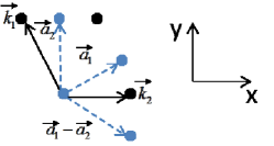
Figure 1: (Color online) The light points and dashed lines show the lattice sites of the atoms and the hopping directions in the triangular lattice respectively, and the dark points and lines are the corresponding Brillouin zone sites and vectors respectively.

In order to calculate the band structure we take the Fourier transform of the Hamiltonian Eq. (II.1). We use the momentum representation of fermionic operator

$$C_{\mathbf{k}}=\sum_{m,n}e^{i\mathbf{k}\cdot\mathbf{R}_{m,n}}C_{m,n},$$ (2)

where $\mathbf{R}_{m,n}=m{\bf{a}}_{1}+n{\bf{a}}_{2}$. We obtain the energy dispersion in triangular lattice by solving the determinant for the eigenvalues $\epsilon$,

$$\mbox{Det}\left[\begin{array}[]{cccc}-A-\epsilon&B+iC&0&0\\ B-iC&A-\epsilon&0&0\\ 0&0&A-\epsilon&B-iC\\ 0&0&B+iC&-A-\epsilon\\ \end{array}\right]=0,$$ (3)

where $A$,$B$ and $C$ are defined to be,

$$A =\cos\left(k_{y}a/2\right),$$ (4)

$$B =\cos\frac{a}{4}\left(\sqrt{3}k_{x}+k_{y}\right),$$ (5)

$$C =\cos\frac{a}{4}\left(\sqrt{3}k_{x}-k_{y}\right).$$ (6)

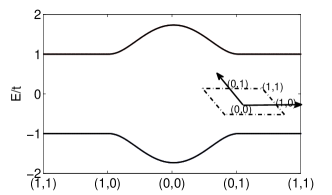
(a)

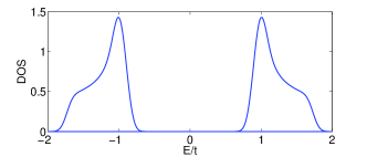
(b)

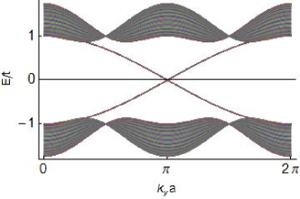
(c)

Figure 2: (Color online) (a) The band structure of the Hamiltonian Eq. (II.1) along the path (1,1), (1,0), (0,0), (0,1) where 1 and 0 are referring to the inset (m,n) in ${\bf{\Gamma}}_{mn}=(m{\bf{k}}_{1}+n{\bf{k}}_{2})$, which are the TRS invariant points in Brillouin zone. The bands are four fold degenerate as in the nearly free electron limit of cold atomic system. (b) The DOS for all the energy bands is shown where the horizontal axis is the energy. (c) The spectrum of the edges of triangular lattice. The shaded area is lowest energy bands for the triangular lattice (for uniform spacing of $-4\pi/\sqrt{3}<k_{x}a<4\pi/\sqrt{3}$). The solid lines show the spin polarized edge state band, traversing the gap. The edge states cross at $k_{y}a=\pi$.

In order to solve Eq. (3), we used a 2D grid for the ${\bf{k}}$-space. Fig.  2a shows the band structure of the Eq.  (3) for a cell with specific ${\bf{k}}$ points as its corners taken to be $(k_{1}+k_{2})/2$, $k_{1}/2$, $0$, $k_{2}/2$, as shown in the inset. These points are the TRS invariant points in the Brillouin zone Since each of the two blocks of the Eq.  (3) corresponds to two fold spin degenerate bands, each band of the Fig.  2a is four fold degenerate.

We also calculated the density of states (DOS) for the Hamiltonian in Eq. (3). This quantity is defined by the expression,

$$\rho(E)=\frac{1}{A}\sum_{\mathbf{k}}\delta(E-E_{n}),$$ (7)

where $A$ is the area of the system in reciprocal space and $E_{n}$ is the energy of the bands. In Fig. 2b the DOS is depicted for all the energy bands.

II.2 Edge-state band structure

The characteristic of the $\mathds{Z}_{2}$ topological insulator is the gapless edge states. They describe two spin currents at the edge, propagating in opposite direction. This property is because of the the time-reversal symmetry and it prevents the gap opening due to any TR invariant perturbation as the result of the Kramer’s theorem  Kane and Mele (2005a).

We follow the method in Ref. Hatsugai (1993) to find the energy dispersion of the edge states. The Hamiltonian Eq. (II.1), must be reduced to a one-dimensional problem. We take the y direction as the periodic part and we use the momentum representation as,

$$C_{m,n}=\frac{1}{\sqrt{L_{y}}}\sum_{k_{y}}e^{ik_{y}n}C_{m}(k_{y}),$$ (8)

where $k_{y}a/2=2\pi n_{y}/L_{y}$, $n_{y}=1,...,L_{y}$ and $L_{y}$ is the system size along $y$ direction. By inserting the single particle state

$$|\Psi(k_{y})\rangle=\sum_{m}|\Psi(k_{y})_{m}\rangle C^{{\dagger}}_{m}(k_{y})|0\rangle$$ (9)

into the Schrödinger equation $H|\Psi\rangle=E|\Psi\rangle$, the spin up part of the problem is reduced to the one-dimensional problem with parameter $k_{y}$ as

$$G^{*}\Psi_{m+1}-G\Psi_{m-1}-2\cos\left(k_{y}a/2-4\pi\phi m\right)\Psi_{m}$$

$$=E\psi_{m}.$$ (10)

where $G=1+e^{-i\left(-k_{y}a/2+\pi\phi\left(2m+1\right)\right)}$. Including the spin down as well, this equation can be written as a generalized Harper equation Harper (1955) in transfer matrix form,

$$\left(\begin{array}[]{c}\Psi_{m+1\uparrow}\left(k_{y}\right)\\ \Psi_{m\uparrow}\left(k_{y}\right)\\ \Psi_{m+1\downarrow}\left(k_{y}\right)\\ \Psi_{m\downarrow}\left(k_{y}\right)\\ \end{array}\right)=M\left(\begin{array}[]{c}\psi_{m\uparrow}\left(k_{y}\right)\\ \psi_{m-1\uparrow}\left(k_{y}\right)\\ \psi_{m\downarrow}\left(k_{y}\right)\\ \psi_{m-1\downarrow}\left(k_{y}\right)\\ \end{array}\right),$$ (11)

where $M$ is the transfer matrix, which is given by:

$$M=\left(\begin{array}[]{cc}\begin{array}[]{cc}\frac{F}{G}&\frac{G^{*}}{G}\\ 1&0\end{array}&0\\ 0&\begin{array}[]{cc}\frac{F^{\prime}}{G^{\prime}}&\frac{G^{\prime*}}{G^{\prime}}\\ 1&0\end{array}\\ \end{array}\right)$$ (18)

with $G^{\prime}=1-e^{-i\left(-k_{y}a/2+\pi\phi\left(2m+1\right)\right)}$, $F=-\epsilon-2\cos\left(k_{y}a/2-4\pi\phi m\right)$ and $F^{\prime}=-\epsilon+2\cos\left(k_{y}a/2-4\pi\phi m\right)$. Under the boundary condition that the wavefunction goes to zero at the boundaries of lattice we can solve this equation. The band structure along the path $k_{y}a=0-2\pi$ is shown in the Fig.  2c. We used 100 k-points along $k_{y}$ direction. The shaded area is the bulk band and the gap traversing edge states as the signature of $\mathds{Z}_{2}$ topological insulator are plotted as the solid line. Since the TRS is preserved no TR symmetric perturbation can open the gap at $k_{y}a=\pi$ Kane and Mele (2005b).

III Cold Atomic system

In this section we review briefly the $\mathds{Z}_{2}$ topological insulator model proposed by Béri and cooper Béri and Cooper (2011). This model is studied in nearly free electron limit which has the advantage of large band gap.

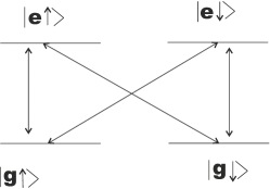
Figure 3: (Color online) The atomic levels of Ytterbium and the interactions between atoms and lasers

The Hamiltonian which describes an atom with position ${\bf{r}}$ and momentum ${\bf{p}}$ and with N internal states is given by

$$H=\frac{{\bf{p}}^{2}}{2m}\mathds{1}_{4}+V\hat{M}({\bf{r}}),$$ (19)

where $V\hat{M}({\bf{r}})$ is a position dependent potential. In order to have a system with low spontaneous emission one can use ytterbium (Yb) which has long-lived excited state. The two internal states, ground state (${}^{1}S_{0}=g$) and long-lived excited state (${}^{3}p_{0}=e$) of Yb have spin degree of freedom which leads to four states Fig.  3. Another interesting aspect of Yb is the existence of a state dependent scalar potential for $\lambda_{\text{magic}}$ with opposite sign $\pm V_{\text{am}}({\bf{r}})$. Therefore we can write the potential part of hamiltonian when we have external electric field as ${\bf{E}}={\bf{\epsilon}}e^{-i\omega t}+{\bf{\epsilon}}^{*}e^{i\omega t}$ with complex amplitude $\epsilon$ and frequency $\omega$. All four e-g transitions have the same frequency $\omega_{0}=(E_{e}-E_{g})/\hbar$. Using rotating wave approximation Cohen-Tannoudji et al. (1992) we have the optical potential as following,

$$V\hat{M}({\bf{r}})=\left(\begin{array}[]{ccc}(\frac{\hbar}{2}\Delta+V_{\text{am}})1&-i{\bf{\sigma}}.{\bf{\epsilon}}d_{r}\\ i{\bf{\sigma}}.{\bf{\epsilon}}d_{r}&-(\frac{\hbar}{2}\Delta+V_{\text{am}})\end{array}\right)\$$ (20)

where $\Delta=\omega-\omega_{0}$ is the atom-field detuning and $d_{r}$ is the dipole moment. One can write the hamiltonian in terms of Dirac matrices  Murakami et al. (2003),

$$\Gamma^{1,2,3}=-i\sigma^{y}\otimes\sigma^{i},\Gamma^{4}=\sigma^{x}\otimes I~{}\text{and}~{}\Gamma^{5}=\sigma^{z}\otimes I,$$ (21)

which gives,

$$H=\frac{\hat{\mathbf{P}}^{2}}{2m}\mathds{1}+\Gamma^{i}d_{r}\epsilon_{i}+\Gamma^{5}(\frac{\hbar}{2}\Delta+V_{\text{am}}).$$ (22)

For the two-dimensional system one can make following choice for the potential matrix Eq. (20):

$$d_{r}\mathbf{\epsilon}=[V\delta,V\cos({\bf{r}}.{\bf{k}}_{1}),V\cos({\bf{r}}.{\bf{k}}_{2})],$$

$$\frac{\hbar}{2}\Delta+V_{am}({\bf{r}})=V\cos({\bf{r}}.({\bf{k}}_{1}+{\bf{k}}_{2}))$$ (23)

with ${\bf{k}}_{1}=k(1,0,0)$ and ${\bf{k}}_{2}=k(\cos(\theta),\sin(\theta),0)$.

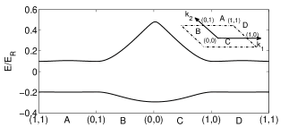
(a)

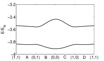
(b)

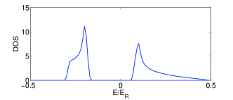
(c)

Figure 4: (Color online) (a) Lowest energy bands of the cold atom system in nearly free electron limit as the result of the solution of Eq. (22). The energy is plotted relative to recoil energy $E_{R}$. $V=0.5E_{R}$ and $\delta=0$ are shown here. The k-points are labeled as ${\bf{\Gamma}}_{mn}=(m{\bf{k}}_{1}+n{\bf{k}}_{2})/2$ and each band is four fold degenerate. (b) Energy bands for the potential $V=3.5E_{R}$ which resembles the band structure of tight binding regime Fig. 2a. (c) DOS of the energy bands in Fig. 2a which are depicted in the band structure is shown. Energy is expressed in the unit of $E_{R}$

The optical potential in Eq. (25) is formed from three standing waves which are linear polarized light at the coupling frequency $\omega$. Two of these waves have equal amplitude in the 2D plane (${\bf{k}}_{1}$ for y polarization and ${\bf{k}}_{2}$ for ${\bf{z}}$ polarization) the ${\bf{x}}$ polarized wave vector is normal to the $2$D plane with an amplitude smaller by a factor of $\delta$. Since the $\omega\simeq\omega_{0}$ , we have $k\simeq 2\pi/\lambda_{0}$ with $\lambda_{0}=578~{}\text{nm}$ the wavelength of the e-g transition. The spatial dependence of $V_{\text{am}}$ is set by a standing wave at the antimagic wavelength $\lambda_{\text{am}}$ Gerbier and Dalibard (2010), which creates a state-dependent potential with $|{\bf{k}}_{1}+{\bf{k}}_{2}|=4\pi/\lambda_{\text{am}}$ that leads $\theta=2\arccos(\pm\lambda_{0}/\lambda_{\text{am}})$. For simplicity, in all following discussions one can fix $\theta=2\pi/3$ and define $a\equiv 4\pi/(\sqrt{3}k)$. Therefore the optical coupling $\hat{M}$ has the symmetry of a triangular lattice. In Fig. 4a we show the few lowest energy bands for $\delta=0$. The bands were calculated by numerical diagonalization in the plane wave basis (49 plane waves is used). All bands are fourfold degenerate similar to tight binding regime.

The relation of this system to the tight binding model given in previous section becomes more clear as one applies the unitary transformation  $\hat{U}=\left(\mathds{1}-i\hat{\Sigma}_{3}\hat{\sigma}_{2}\right)/\sqrt{2}$ to the coupling $\hat{M}$ in Eq. (20):

$$\hat{M^{\prime}}=\hat{U}^{{\dagger}}\hat{M}\hat{U}=c_{1}\hat{\Sigma}_{1}+c_{2}\hat{\Sigma}_{2}\sigma_{3}+c_{12}\hat{\Sigma}_{3},$$ (24)

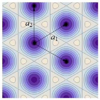
Figure 5: (Color online) The dark circles show the local minima of the adiabatic energy which forms a triangular lattice in the tight binding limit.

here $\Sigma_{i}=\sigma_{i}\otimes\mathds{1}_{2\times 2}$, $c_{i}\equiv\cos(\mathbf{r}\cdot\mathbf{k_{i}})$ and $c_{12}=\cos\left(\mathbf{r}\cdot\left(\mathbf{k}_{1}+\mathbf{k}_{2}\right)\right)$. This matrix is $2\times 2$ block diagonal matrix for each eigenvalue of $\sigma_{3}$ ( since the kinetic part is diagonal this is the case for the Hamiltonian as well) thus the four level system decouples into two two level system each of which experiences an effective magnetic field due to the optical dressed state of the $c_{1}\hat{\Sigma}_{1}+\pm c_{2}\hat{\Sigma}_{2}+c_{12}\hat{\Sigma}_{3}$  Cooper (2011). This means that opposite spin direction undergoes an effective magnetic field of the same strength but with opposite signs. Beside the lowest band energy of these systems have $\pm 1$ Chern number which they cancel out each other because of the time-reversal symmetry. These are the required criteria for the quantum spin Hall effect.

To make the connection to the previous section we consider the adiabatic limit $V\gg\hbar k^{2}/2M$ Dalibard et al. (2011) when the potential part of the Hamiltonian Eq. (19) plays the dominant role. In order to find the minima of the adiabatic energy which gives the lattice sites in tight binding regime  Jaksch and Zoller (2005) we diagonalized the potential in Eq.  (24) analytically and obtained,

$$V_{\text{ad}}=\pm\sqrt{c_{1}^{2}+c_{2}^{2}+c_{12}^{2}},$$ (25)

as plotted in Fig. 5. Now if we ignore the spin here, the effective magnetic field strength experienced by the neutral atom following the adiabatic path is equivalent to the $1/4$ of a flux quantum that a charged particle acquires enclosing the elementary plaquette of the triangular lattice in tight binding limit  Cooper (2011). This is equivalent to the Hamiltonian Eq. (II.1) proposed in this paper without spin. Therefore tight binding limit of the ultra cold atomic system of Ref. Béri and Cooper (2011) is given in Eq. (II.1) and the hopping parameter $t$ is related to the potential scale of optical coupling $V$ based on the formalism in Jaksch et al. (1998). The difference is in the $(0,0)$ point in k-space where the upper band of cold atom limit has a sharper peak Fig. 4a than the tight binding upper band Fig 2a. This can be understood as the characteristic behavior of the energy levels of free electron which are just a parabola in k (momentum), by getting distorted due to a periodic potential Ashcroft and Mermin (1976). As the potential becomes stronger the energy dispersion resembles the tight binding regime Fig. 4b. The DOS for the nearly free electron limit is also depicted in Fig. 4c which shows that states are distributed around the two energy bands across the gap asymmetrically due to the asymmetrically located van Hove singularities of the upper and lower bands in contrast to that of tight binding case in Fig. 2b. Finally we note that realization of QSH models in Eq. (II.1) and Eq. (19) does not require any spin flipping interactions and thus does not need any additional cooling mechanism Kennedy et al. (2013).

IV Conclusion

Summarising, we considered the quantum spin Hall effect on the triangular lattice in the tight binding limit and we proposed that this can be realized in the ultra cold atomic system. We studied the edge state band structure which reveals the $\mathds{Z}_{2}$. The nearly free electron limit of the system we proposed here is introduced as $\mathds{Z}_{2}$ topological insulator in Ref. Béri and Cooper (2011).