A statistical approach to the inverse problem in magnetoencephalography

Abstract

Magnetoencephalography (MEG) is an imaging technique used to measure the magnetic field outside the human head produced by the electrical activity inside the brain. The MEG inverse problem, identifying the location of the electrical sources from the magnetic signal measurements, is ill-posed, that is, there are an infinite number of mathematically correct solutions. Common source localization methods assume the source does not vary with time and do not provide estimates of the variability of the fitted model. Here, we reformulate the MEG inverse problem by considering time-varying locations for the sources and their electrical moments and we model their time evolution using a state space model. Based on our predictive model, we investigate the inverse problem by finding the posterior source distribution given the multiple channels of observations at each time rather than fitting fixed source parameters. Our new model is more realistic than common models and allows us to estimate the variation of the strength, orientation and position. We propose two new Monte Carlo methods based on sequential importance sampling. Unlike the usual MCMC sampling scheme, our new methods work in this situation without needing to tune a high-dimensional transition kernel which has a very high cost. The dimensionality of the unknown parameters is extremely large and the size of the data is even larger. We use Parallel Virtual Machine (PVM) to speed up the computation.

and t1Supported in part by NSF SES-1061387 and NIH/NIDA R90 DA023420.

1 Introduction

1.1 The basics of magnetoencephalography (MEG)

The anatomy of the brain has been studied intensively for millennia, yet how the brain functions is still not well understood. The neurons in the brain produce macroscopic electrical currents when the brain functions, and those synchronized neuronal currents in the gray matter of the brain induce extremely weak magnetic fields (10–100 femto-Tesla) outside the head. The comparatively recent development of the Superconducting Quantum Interference Device (SQUID) makes it possible to detect those magnetic signals. MEG is an imaging technique using SQUIDs to measure the magnetic signals outside of the head produced by the electrical activity inside the brain [Cohen (1968)]. The primary sources are electric currents within the dendrites of the large pyramidal cells of activated neurons in the human cortex, generally formulated as a mathematical point current dipole. Such focal brain activation can be observed in epilepsy, or it can be induced by a stimulus in neurophysiological or neuropsychological experiments. Due to its noninvasiveness (it is a completely passive measurement method) and its impressive temporal resolution (better than 1 millisecond, compared to 1 second for functional magnetic resonance imaging, or to 1 minute for positron emission tomography), and due to the fact that the signal it measures is a direct consequence of neural activity, MEG is a near optimal tool for studying brain activity, such as assisting surgeons in localizing a pathology, assisting researchers in determining brain function, neuro-feedback and others. The skull and the tissue surrounding the brain affect the magnetic fields measured by MEG much less than the electrical impulses measured by electroencephalography (EEG). This means that MEG has higher localization accuracy than the EEG and it allows for a more reliable localization of brain function [Hämäläinen et al. (1993), Okada, Lähteenmäki and Xu (1999)]. MEG has recently been used in the evaluation of epilepsy, where it reveals the exact location of the abnormalities, which may then allow physicians to find the cause of the seizures [Barkley and Baumgartner (2003)]. MEG is also reference free, so that the localization of sources with a given precision is easier for MEG than it is for EEG [Kristeva-Feige et al. (1997)]. The computation associated with estimating the electric source from the magnetic measurement is a challenging problem that needs to be solved to allow high temporal and spatial resolution imaging of the dynamic activity of the human brain.

1.2 Forward and inverse MEG problem

The MEG signals derive from the primary current (the net effect of ionic currents flowing in the dendrites of neurons) and the volume current (i.e., the additive ohmic current set up in the surrounding medium to complete the electrical circuit). If the electrical source is known and the head model [Kybic et al. (2006)] is specified (e.g., a sphere with homogeneous conductivity), then the “forward problem” is to compute the electric field $\mathbf{E}$ and the magnetic field $\mathbf{B}$ from the source current $\mathbf{J}$. The calculation uses Maxwell’s equations [see, e.g., Griffiths (1999)],

$$\nabla\cdot\mathbf{E} = \rho/\varepsilon_{0},$$

$$\nabla\times\mathbf{E} = -\partial\mathbf{B}/\partial t,$$

$$\nabla\cdot\mathbf{B} = 0,$$

$$\nabla\times\mathbf{B} = \mu_{0}(\mathbf{J}+\varepsilon_{0}\,\partial\mathbf{E}/\partial t),$$

where $\varepsilon_{0}$ and $\mu_{0}$ are the permittivity and permeability of a vacuum, respectively, and $\rho$ is the charge density. The total current $\mathbf{J}$ consists of the primary current $\mathbf{J}^{\mathrm{P}}$ plus the volume current $\mathbf{J}^{\mathrm{V}}$. The source activity in the brain corresponds to the primary current. Under reasonable assumptions [see Hämäläinen et al. (1993)], the volume current $\mathbf{J}^{\mathrm{V}}$ is not included in the analysis because of its diffuse nature. The terms $\partial\mathbf{B}/\partial t$ and $\partial\mathbf{E}/\partial t$ in Maxwell’s equations can be ignored by assuming that the magnetic field varies relatively slowly in time. Rather than working with continuous electric current, the most frequently used computational model assumes that the electric current can be thought of as an electric dipole; this model is called an equivalent current dipole (ECD); see, for example, Hämäläinen et al. (1993). From the perspective of an ECD, a dipole has location, orientation and magnitude; the magnetic field generated by this dipole can explain the MEG measurements. In addition, there is a version of an ECD model assuming multiple dipoles; from Maxwell’s equations it is easy to see that this model is simply the sum of the models for each ECD. Such an ECD models a large number of dipoles located at fixed places over the cortical surface. In neuroscience, it is believed that typical MEG data should be explained by only a few dipoles (less than 10), and different criteria or algorithms are used to minimize the number of dipoles in various ECD models; we discuss some of these models in Section 1.3. We assume that $\mathbf{E}$ is generated by $\mathbf{J}^{\mathrm{P}}$, which in turn comes from the sum of $N$ localized current dipoles at locations $\mathbf{r}_{n}$,

$$\mathbf{J}_{n}^{\mathrm{P}}(\mathbf{r})=Q_{n}\delta(\mathbf{r}-\mathbf{r}_{n}),\qquad n=1,\ldots,N,$$

where $\delta(\cdot)$ is the Dirac delta function. The $Q_{n}$ is a charged dipole at the point $\mathbf{r}_{n}$ in the brain volume $\Omega$. Using the quasi-static approximation to Maxwell’s equations (i.e., ignoring the partial derivatives with respect to time) given in Sarvas (1984), the magnetic field $\mathbf{B}$ at location $\mathbf{r}$ of a current dipole at $\mathbf{r}_{n}$ can be calculated by the Biot–Savart equation,

$$\mathbf{B}_{n}(\mathbf{r})=\frac{\mu_{0}}{4\pi}\int_{\Omega}\frac{\mathbf{J}^{\mathrm{P}}(\mathbf{r}_{n})\times(\mathbf{r}-\mathbf{r}_{n})}{|\mathbf{r}-\mathbf{r}_{n}|^{3}}\,d\mathbf{r}_{n}.$$

In the case of multiple current dipoles, the induced magnetic fields simply add up.

The “inverse problem” comes from the forward model; we want to estimate the dipole parameters from the observed magnetic signal. The difficulty is that there is not a unique solution; there are infinitely many different sources within the skull that produce the same observed data. The goal is to find a meaningful solution among the many mathematically correct solutions. There are three key steps to any source localization algorithm in MEG. First, define the solution space and the parameter space of the electric source. Second, calculate the magnetic field given the information about the head model. Third, according to what criterion the solution must satisfy, perform an extensive search for the solution. Methods of finding the source from the observed MEG signal have been extensively exploited during the past two decades, mostly centered on finding a single estimate of the source. Some of these methods are briefly described in the next subsection. However, finding the distribution of the source in space and (particularly) in time is still a problem requiring investigation.

1.3 Existing source localization methods

Most methods for localizing electrical sources in MEG assume that the electrical sources in the brain do not include a temporal component. The data are used to estimate the source parameters at each time point; there is no relation to the estimates for the previous time. This is not the same as assuming the quasi-static approximation to Maxwell’s equations. Therefore, those existing methods are restricted to fixed dipole assumptions and are also not able to provide estimates of the variability of source activity. The minimum norm estimate (MNE) [Hämäläinen and Ilmoniemi (1994)] is a regularization method based on the $L_{2}$ norm. The $L_{1}$ norm regularization yields the minimum current estimates (MCE) [Uutela, Hämäläinen and Somersalo (1999)]. The LORETA approach [Mattout et al. (2006)] is a special case of weighted MNE. The Multiple Signal Classification method (MUSIC) [Mosher, Lewis and Leahy (1992)] searches for a single-dipole model through a three-dimensional head volume and computes projections onto an estimated signal subspace. The source locations are then found as the 3-D locations where the source model gives the best projections onto the subspace. The beamformer methods [Van Veen, Joseph and Hecox (1992)] ignore the ill-posed inverse problem and instead only estimate the current at several fixed locations. Bayesian approaches to the MEG inverse problem try to find the posterior distribution of the dipole parameters [Bertrand et al. (2001), Schmidt, George and Wood (1999)].

The methods mentioned briefly above (MNE, MCE, etc.) have been widely used and produce apparently meaningful solutions; however they have overly restrictive assumptions and lack estimates of the variability of source estimates. By assuming a static localized dipole, these methods are limited in their ability to incorporate problem-specific anatomical or physiological information. It is quite reasonable to consider that the source is time-varying rather than fixed, in which case the noise reduction obtained by averaging over consecutive observations in time is problematic. By utilizing a time-varying source model, we will be able to investigate the distribution of the source at each time point and provide estimates of the variability. Following this idea, the time evolution of the source is modeled by a state space model. Our goal is to find the posterior distribution of the source parameters. Our reformulation of the inverse problem leads to a predictive model of the dipole. It turns out that the posterior source distribution from our predictive model can be interpreted as a statistical solution to the MEG inverse problem.

1.4 Outline of this paper

In Section 2 we develop a time-varying source model for the MEG inverse problem. Rather than attempting to “solve” the inverse problem we try to develop estimates of the dipole parameters using a spatio-temporal model. In Section 3 the difficulty of using Markov chain Monte Carlo (MCMC) methods for generating samples from the time-varying model is explained. Then, we introduce the standard Sequential Importance Sampling (SIS) technique. Next, two further Monte Carlo methods are described: (1) the regular SIS method with rejection, and (2) the improved SIS method with resampling. A simulation study is described in Section 4. We describe our use of the Parallel Virtual Machine (PVM) software to speed up the computations in Section 4.2. We believe this is the first application of parallel computational methods to the problem. In Section 5 a real data application is presented. Section 6 contains a short discussion and conclusion.

2 A probablistic rime-varying source model

Assume that the magnetic field data is measured from the $k$th sensor at time $t$ as

$$Y_{k,t}=\mathbf{B}_{k}\bigl{(}\mathbf{J}^{\mathrm{P}}_{t}\bigr{)}+\mathbf{U}_{k,t},\qquad 1\leq t\leq T,1\leq k\leq L,$$

where $\mathbf{U}_{k,t}\sim N(0,\sigma_{1}^{2})$ denotes the observation noise that is assumed, for simplicity, to be Gaussian, additive and homogeneous for all the sensors, and uncorrelated between every pair of sensors. The assumption of normality is preferred due to the fact that Gaussian sensor noise is present at the MEG sensors themselves, and sensor noise is typically substantially smaller than signals from spontaneous brain activity [Hämäläinen et al. (1993)]. Although correlated sensor noise is more realistic than “homogeneous” sensors, it complicates the problem. Background noise and biological noise can also drown out the brain activity of interest, but these are all very difficult to incorporate. Besides some variation coming from solving the inverse problem, most of the variation of the source localization in MEG is due to the propagation of errors through Maxwell’s equations when solving the forward problem. In order to control variation, we only work with a simple sensor structure. Therefore, we write

$$\mathbf{Y}_{t}=\mathbf{B}\bigl{(}\mathbf{J}^{\mathrm{P}}_{t}\bigr{)}+\mathbf{U}_{t},\qquad 1\leq t\leq T,$$

where $\mathbf{Y}_{t}=(Y_{1,t},\ldots,Y_{L,t})^{T}$, $\mathbf{B}(\mathbf{J}^{\mathrm{P}}_{t})=(\mathbf{B}_{1}(\mathbf{J}^{\mathrm{P}}_{t}),\ldots,\mathbf{B}_{L}(\mathbf{J}^{\mathrm{P}}_{t}))^{T}$ and $\mathbf{U}_{t}=(\mathbf{U}_{1,t},\break\ldots,\mathbf{U}_{L,t})^{T}$. Here, $\mathbf{U}_{t}\sim\mathcal{N}(\mathbf{0},\bolds{\Sigma}_{1})$, where $\bolds{\Sigma}_{1}=\operatorname{diag}[\sigma_{1}^{2},\ldots,\sigma_{1}^{2}]$.

The $\mathbf{B}_{k}(\mathbf{J}_{t}^{\mathrm{P}})$, a function of the dipole with parameter vector $\mathbf{J}_{t}^{\mathrm{P}}$, is the physical approximation of the Biot–Savart law in Section 1.2. We consider a current dipole located within a horizontally layered conductor [Hämäläinen et al. (1993)]. The noiseless magnetic field at the $k$th sensor, $\mathbf{B}_{k}$, is computed from the source $\mathbf{J}_{t}^{\mathrm{P}}=(\mathbf{p}_{t},\mathbf{q}_{t})$ at time $t$. The vector $\mathbf{p}_{t}=({p_{1}}_{t},{p_{2}}_{t},{p_{3}}_{t})$ contains the location parameters of the source and the vector $\mathbf{q}_{t}=({q_{1}}_{t},{q_{2}}_{t},{q_{3}}_{t})$ contains the moments and strength. Thus,

$$\mathbf{B}_{k}\bigl{(}\mathbf{J}^{\mathrm{P}}_{t}\bigr{)}=\frac{\mu_{0}}{4\pi}\frac{\mathbf{q}_{t}\times(\mathbf{r}_{k}-\mathbf{p}_{t})\cdot\mathbf{e}}{|\mathbf{r}_{k}-\mathbf{p}_{t}|^{3}}.$$ (1)

Here, $\mathbf{r}_{k}$ is the location of the $k$th sensor. Because the magnetometers measure only the $z$ direction of the magnetic field $\mathbf{B}$, $\mathbf{e}=(0,0,1)$, a unit vector, is used to find the $z$ component of $\mathbf{B}$. Conventionally, $z$ is perpendicular to the surface of the skull.

To specify the prior, the time evolution of the current dipole $\mathbf{J}^{\mathrm{P}}_{t}$ is modeled by a state space model. A number of other authors have also proposed stating the MEG inverse problem as a Bayesian dynamic model; see Somersalo, Voutilainen and Kaipio (2003); Campi et al. (2008, 2011); Sorrentino et al. (2009, 2013); Miao et al. (2013). We could choose any of a large variety of state space models but, for theoretical and computational simplicity, we have chosen a six-dimensional first-order autoregression:

$$\mathbf{J}^{\mathrm{P}}_{t}=\mathbf{m}_{\mathrm{com}}+\bolds{\rho}\bigl{(}\mathbf{J}^{\mathrm{P}}_{t-1}-\mathbf{m}_{\mathrm{com}}\bigr{)}+\mathbf{V}_{t},\qquad 1\leq t\leq T,$$

where $\mathbf{V}_{t}\sim\mathcal{N}(\mathbf{0},\bolds{\Sigma}_{2})$ denotes the state evolution noise. We note that three of the parameters give the spatial location, so this is implicitly a space–time model. Previous work using a space–time model [Ou, Hämäläinen and Golland (2009)] used a novel mixed $L_{1}L_{2}$-norm estimate for the dipole parameters based on a linear regression model. Jun et al. (2005) have also used MCMC methods for sampling from the posterior of a spatiotemporal Bayesian dynamic model. To reduce the number of parameters, and hence the amount of variation in our estimates, we assume the dipole parameters are uncorrelated. That is, we assume that $\bolds{\Sigma}_{2}=\operatorname{diag}[\sigma_{11}^{2},\sigma_{22}^{2},\ldots,\sigma_{66}^{2}]$ is a known $6$ by $6$ diagonal matrix and $\sigma_{ii}^{2}$ is the variance of the $i$th source parameter. The parameter vector $\mathbf{m}_{\mathrm{com}}$ is a constant associated with the source $\mathbf{J}^{\mathrm{P}}_{t}$ for $1\leq t\leq T$. The initial state is chosen as $\mathbf{J}^{\mathrm{P}}_{0}\sim\mathcal{N}(\mathbf{m}_{\mathrm{ini}},\bolds{\Sigma}_{2})$, where $\mathbf{m}_{\mathrm{ini}}$ is also a constant parameter vector. Both $\mathbf{m}_{\mathrm{ini}}$ and $\mathbf{m}_{\mathrm{com}}$ are specified in advance. The known diagonal matrix $\bolds{\rho}=\operatorname{diag}[\rho_{1},\rho_{2},\ldots,\rho_{6}]$ is $6$ by $6$. Its main diagonal represents the autoregressive coefficients. Hence, at any time $t$, $\mathbf{J}^{\mathrm{P}}_{t}$ or $(\mathbf{p}_{t},\mathbf{q}_{t})$ contains the parameters of interest and $\mathbf{Y}_{t}=(Y_{1,t},\ldots,Y_{L,t})$ is the (very noisy) data collected from all sensors. Both $\{\mathbf{J}^{\mathrm{P}}_{t}\}_{t=0}^{T}$ and $\{Y_{k,t}\}_{t=1}^{T}$ are assumed to have the following Markov properties: [(iii)]

The $\mathbf{J}^{\mathrm{P}}$ is a first order Markov process. The distribution of each state $\mathbf{J}^{\mathrm{P}}_{t}$ only depends on its own previous state $\mathbf{J}^{\mathrm{P}}_{t-1}$,

$$p\bigl{(}\mathbf{J}^{\mathrm{P}}_{t}|\mathbf{J}^{\mathrm{P}}_{0},\mathbf{J}^{\mathrm{P}}_{1},\ldots,\mathbf{J}^{\mathrm{P}}_{t-1}\bigr{)}=p\bigl{(}\mathbf{J}^{\mathrm{P}}_{t}|\mathbf{J}^{\mathrm{P}}_{t-1}\bigr{)}$$ (2)

(we are using $p$ as a generic symbol for a probability distribution; the two $p$’s in this equation are not the same function).

The process $Y_{k,t}$ (for any $1\leq k\leq L$) is also a Markov process with respect to the history of $\mathbf{J}^{\mathrm{P}}$. The density of $Y_{k,t}$ conditioned on $\{\mathbf{J}^{\mathrm{P}}_{t}\}_{0}^{t}$ satisfies

$$f\bigl{(}Y_{k,t}|\mathbf{J}^{\mathrm{P}}_{0},\mathbf{J}^{\mathrm{P}}_{1},\ldots,\mathbf{J}^{\mathrm{P}}_{t}\bigr{)}=f\bigl{(}Y_{k,t}|\mathbf{J}^{\mathrm{P}}_{t}\bigr{)}$$

(again $f$ is a generic symbol, in this case, for a joint density function).

When conditioned on its own history, the unknown $\mathbf{J}^{\mathrm{P}}_{t}$ does not depend on past measurements. The distribution of $\mathbf{J}^{\mathrm{P}}_{t}$ based on $\mathbf{Y}^{k}=(Y_{k,1},\ldots,\break Y_{k,t-1})$ and $\mathbf{J}^{\mathrm{P}}_{t-1}$ is

$$g\bigl{(}\mathbf{J}^{\mathrm{P}}_{t}|\mathbf{J}^{\mathrm{P}}_{t-1},\mathbf{Y}^{k}\bigr{)}=p\bigl{(}\mathbf{J}^{\mathrm{P}}_{t}|\mathbf{J}^{\mathrm{P}}_{t-1}\bigr{)},\qquad t>0$$ (3)

[the right-hand side of equation (3) in (iii) is the same as the right-hand side of equation (2) in (i)]. The transition kernel, $p(\mathbf{J}^{\mathrm{P}}_{t}|\mathbf{J}^{\mathrm{P}}_{t-1})$, is defined here as a first order Markov process in the state space model above. For a more complex model it could be a higher order Markov process. The choice of more realistic models for this process [e.g., in the situation where the magnetic signal is a response to a stimulus, the source variance might change much more rapidly immediately after the stimulus than before it; the joint density $f(Y_{k,t}|\mathbf{J}^{\mathrm{P}}_{t})$ for any $1\leq k\leq L$ may also vary in time since not all the measurements can be carried out simultaneously] is not the aim of this paper.

Of interest at any time $t$ is the posterior distribution of $\mathcal{J}^{\mathrm{P}}_{t}=(\mathbf{J}^{\mathrm{P}}_{0},\ldots,\mathbf{J}^{\mathrm{P}}_{t})$. Let $\mathcal{Y}_{\mathrm{obs}}^{t}=(\mathbf{Y}_{1},\ldots,\mathbf{Y}_{L})=({Y_{1,1},\ldots,Y_{1,t}},\dots,{Y_{L,1},\ldots,Y_{L,t}})$ be the magnetic measurements, accordingly. By taking all the previous prior information and the three assumptions [(i), (ii), (iii)] above into account, our problem can be stated as finding the target distribution, $p(\mathcal{J}^{\mathrm{P}}_{t}|\mathcal{Y}_{\mathrm{obs}}^{t})$, given $\mathcal{Y}_{\mathrm{obs}}^{t}$. By Bayes’ theorem, we have

$$p\bigl{(}\mathcal{J}^{\mathrm{P}}_{t}|\mathcal{Y}_{\mathrm{obs}}^{t}\bigr{)} \propto f\bigl{(}\mathcal{Y}_{\mathrm{obs}}^{t}|\mathcal{J}^{\mathrm{P}}_{t}\bigr{)}p\bigl{(}\mathcal{J}^{\mathrm{P}}_{t}\bigr{)}$$

$$= \Biggl{[}\prod_{s=1}^{t}\prod_{k=1}^{L}f\bigl{(}Y_{k,s}|\mathbf{J}^{\mathrm{P}}_{s}\bigr{)}\Biggr{]}\Biggl{[}\prod_{s=1}^{t}p\bigl{(}\mathbf{J}^{\mathrm{P}}_{s}|\mathbf{J}^{\mathrm{P}}_{s-1}\bigr{)}\Biggr{]}p\bigl{(}\mathbf{J}^{\mathrm{P}}_{0}\bigr{)}.$$

This framework is based on a one-source model ($N=1$). It can be easily extended to a multiple-source model because the fields generated by distinct sources simply add up. Because it is a high-dimensional distribution ($1\leq t\leq T$, $T$ is very large) and inherently complicated, sampling from the posterior is difficult. We have chosen to use MCMC methods but they are also complex and are very hard to implement. As we will show later, obtaining $p(\mathcal{J}^{\mathrm{P}}_{t}|\mathcal{Y}_{\mathrm{obs}}^{t})$ can be achieved dynamically by computing the $p(\mathbf{J}^{\mathrm{P}}_{u}|\mathcal{Y}_{\mathrm{obs}}^{u})$ at each time point $1\leq u\leq t$. These calculations have to be repeated for each $t\leq T$.

3 Solving the MEG inverse problem

3.1 The difficulty of solving the time-varying model

A problem with MCMC methods (e.g., Metropolis–Hastings) for getting joint posterior samples from $p(\mathcal{J}^{\mathrm{P}}_{t}|\mathcal{Y}_{\mathrm{obs}}^{t})$ occurs when there are a large number of states because it is difficult to find a joint transition kernel which could be used in an MCMC sampler. However, the goal of getting $p(\mathcal{J}^{\mathrm{P}}_{t}|\mathcal{Y}_{\mathrm{obs}}^{t})$ can be achieved by sampling from the distribution $p(\mathbf{J}^{\mathrm{P}}_{s}|\mathcal{Y}_{\mathrm{obs}}^{s})$ for each state $s$ ($1\leq s\leq t$) separately and the entire outcome could be regarded as the sample from the joint distribution. Gibbs sampling can be used for this restricted goal, but because of the nonlinearity of the model [equation (1)], it is not easy to sample from $p(\mathbf{J}^{\mathrm{P}}_{t}|\mathbf{J}^{\mathrm{P}}_{s\neq t},\mathcal{Y}_{\mathrm{obs}}^{t})$. One way to alleviate the difficulty is to insert some kind of Metropolis sampler into a Gibbs sampling scheme for each conditional distribution. When we insert a random-walk Metropolis algorithm, where the move depends only on its own state, into the Gibbs sampler, we call it a random-walk MCMC within Gibbs sampler, and when we insert a hybrid Metropolis algorithm, where the move may depend on other states, into the Gibbs sampler, we call it a hybrid MCMC within Gibbs sampler.

The key to random-walk MCMC within Gibbs is to propose a candidate $\mathbf{J}^{\mathrm{P}^{*}}_{t}\sim\mathcal{N}(\mathbf{J}^{\mathrm{P}}_{t},\bolds{\Sigma}_{3})$ for each $t$ ($1\leq t\leq T$), where $\bolds{\Sigma}_{3}=\operatorname{diag}[\tau_{1}^{2},\tau_{2}^{2},\ldots,\tau_{6}^{2}]$ is a $6$ by $6$ diagonal matrix, and accept $\mathbf{J}^{\mathrm{P}^{*}}_{t}$ if the acceptance ratio

$$\alpha_{t}=\frac{\prod_{k=1}^{L}f(Y_{k,t}|\mathbf{J}^{\mathrm{P}^{*}}_{t})p(\mathbf{J}^{\mathrm{P}^{*}}_{t}|\mathbf{J}^{\mathrm{P}}_{t-1})p(\mathbf{J}^{\mathrm{P}}_{t+1}|\mathbf{J}^{\mathrm{P}^{*}}_{t})}{\prod_{k=1}^{L}f(Y_{k,t}|\mathbf{J}^{\mathrm{P}}_{t})p(\mathbf{J}^{\mathrm{P}}_{t}|\mathbf{J}^{\mathrm{P}}_{t-1})p(\mathbf{J}^{\mathrm{P}}_{t+1}|\mathbf{J}^{\mathrm{P}}_{t})}\geq\mathcal{U}(0,1),$$

where $\mathcal{U}(0,1)$ is the uniform distribution. The problem is that $\mathcal{N}(\mathbf{J}^{\mathrm{P}}_{t},\bolds{\Sigma}_{3})$ is not a good proposal for $\mathbf{J}^{\mathrm{P}^{*}}_{t}$ (i.e., we almost always reject the proposal) and this can not be solved by extensively tuning $\bolds{\Sigma}_{3}=\operatorname{diag}[\tau_{1}^{2},\tau_{2}^{2},\ldots,\tau_{6}^{2}]$ in most practical cases if the dimension of the states is very high. A local linear approximation might be considered, such as performing a Taylor expansion on the joint density function $f({Y}_{k,t}|\mathbf{J}^{\mathrm{P}}_{t})$ and truncating high order terms. The resultant can then be incorporated into the proposal distribution. However, such linearization is not easy due to the highly complex function $f({Y}_{k,t}|\mathbf{J}^{\mathrm{P}}_{t})$; moreover, the extra work of a Taylor expansion might be unnecessary if we only need an efficient sampling scheme in high dimensions.

The hybrid MCMC within Gibbs improves upon the random-walk MCMC within Gibbs when the target distribution is not able to be captured by a simple random walk. In Gelman, Roberts and Gilks (1996), a full conditional prior (hybrid MCMC) was proposed. Similar work can also be found in Carter and Kohn (1994), where a single move blocking strategy was developed but bad convergence behavior was discovered. Gamerman (1998) suggested a reparameterization of the model to a prior independent system of disturbances and built a proposal by a weighted least squares algorithm, however, the reparameterization resulted in quadratic computational time. Knorr-Held (1999) suggested an autoregressive prior where the “conditional prior” is drawn independently of the current state but, in general, depends on other states. Here, our hybrid MCMC within Gibbs is built on a single move proposal, that is, $\mathbf{J}^{\mathrm{P}^{*}}_{t}$ is proposed from the distribution of $p(\mathbf{J}^{\mathrm{P}}_{t}|\mathbf{J}^{\mathrm{P}}_{s\neq t})$ which can be further reduced to $p(\mathbf{J}^{\mathrm{P}}_{t}|\mathbf{J}^{\mathrm{P}}_{t-1},\mathbf{J}^{\mathrm{P}}_{t+1})$ due to the Markov property. One way to update $\mathbf{J}^{\mathrm{P}}_{t}$ is to use a proposal

$$\mathbf{J}^{\mathrm{P}^{*}}_{t}\sim\mathcal{N}\bigl{(}\bolds{\rho}\bigl{(}\mathbf{J}^{\mathrm{P}}_{t-1}-\mathbf{J}^{\mathrm{P}}_{t+1}\bigr{)}+\bigl{(}\mathbf{I}-\bolds{\rho}\bolds{\rho}^{\prime}\bigr{)}\bigl{(}\mathbf{I}+\bolds{\rho}\bolds{\rho}^{\prime}\bigr{)}^{-1}\mathbf{m}_{\mathrm{com}},\bolds{\Sigma}_{2}\bigl{(}\mathbf{I}+\bolds{\rho}\bolds{\rho}^{\prime}\bigr{)}^{-1}\bigr{)}.$$

The acceptance ratio then reduces to

$$\alpha_{t}=\frac{\prod_{k=1}^{L}f(Y_{k,t}|\mathbf{J}^{\mathrm{P}^{*}}_{t})}{\prod_{k=1}^{L}f(Y_{k,t}|\mathbf{J}^{\mathrm{P}}_{t})}.$$

The performance of a single move could be extended to a block move by sampling a block of states at the same time based on other states. Similarly, the $\mathbf{J}^{\mathrm{P}^{*}}_{r},\ldots,\mathbf{J}^{\mathrm{P}^{*}}_{s}$ come from the conditional proposal

$$p\bigl{(}\mathbf{J}^{\mathrm{P}}_{r},\ldots,\mathbf{J}^{\mathrm{P}}_{s}|\mathbf{J}^{\mathrm{P}}_{1,\ldots,T}/\bigl{(}\mathbf{J}^{\mathrm{P}}_{r},\ldots,\mathbf{J}^{\mathrm{P}}_{s}\bigr{)}\bigr{)},$$

where $r<s$ and $\mathbf{J}^{\mathrm{P}}_{1,\ldots,T}/(\mathbf{J}^{\mathrm{P}}_{r},\ldots,\mathbf{J}^{\mathrm{P}}_{s})$ means a collection of $\mathbf{J}^{\mathrm{P}}_{1},\ldots,\mathbf{J}^{\mathrm{P}}_{r-1},\mathbf{J}^{\mathrm{P}}_{s+1},\break\ldots,\mathbf{J}^{\mathrm{P}}_{T}$. Thus, the acceptance ratio becomes

$$\alpha_{t}=\frac{\prod_{k=1}^{L}\prod_{t=r}^{s}f(Y_{k,t}|\mathbf{J}^{\mathrm{P}^{*}}_{t})}{\prod_{k=1}^{L}\prod_{t=r}^{s}f(Y_{k,t}|\mathbf{J}^{\mathrm{P}}_{t})}.$$

Although the block move provides a considerable improvement in the situation where a single move has poor mixing behavior, Carter and Kohn (1994) observed bad mixing and convergence behavior in the blocking strategy.

Recently developed adaptive samplers [Andrieu and Thoms (2008), Roberts and Rosenthal (2009)] might help find the transition kernel within a Gibbs sampler, but these methods are computationally inefficient in high dimension. In addition, although parallel tempering [Srinivasan (2002)] seems reasonable, finding the temperature is not straightforward and significantly increases the computational cost. Again, the MEG data set is extremely large; in particular, we collect hundreds of channels of data at each time and we collect data for hundreds of thousands of time points. It is quite difficult to implement these methods since even a simple model has an extremely large number of states. The computational burden is even more substantial in the multiple-dipole case.

3.2 Sequential importance sampling (SIS)

Sequential importance sampling (SIS) [Liu and Chen (1998)] is advocated as a more practical tool for a dynamic system. As we mentioned briefly in Section 2, computing $p(\mathbf{J}^{\mathrm{P}}_{u}|\mathcal{Y}^{u}_{\mathrm{obs}})$ sequentially in $u$ for $1\leq u\leq t$ can lead to $p(\mathcal{J}^{\mathrm{P}}_{t}|\mathcal{Y}_{\mathrm{obs}}^{t})$. Consider $\pi_{t}(\mathbf{J}^{\mathrm{P}}_{t})=p(\mathbf{J}^{\mathrm{P}}_{t}|\mathcal{Y}^{t}_{\mathrm{obs}})$; calculating $p(\mathcal{J}^{\mathrm{P}}_{t}|\mathcal{Y}_{\mathrm{obs}}^{t})$ or, equivalently, $\pi_{t}(\mathcal{J}^{\mathrm{P}}_{t})$ can be achieved by performing the following two processes in sequential order:

$$\pi_{t}\bigl{(}\mathbf{J}^{\mathrm{P}}_{t}\bigr{)} = \frac{f(\mathbf{Y}_{t}|\mathbf{J}^{\mathrm{P}}_{t})\pi_{t-1}(\mathbf{J}^{\mathrm{P}}_{t})}{\pi_{t-1}(\mathbf{Y}_{t})},$$ (5)

$$\pi_{t}\bigl{(}\mathbf{J}^{\mathrm{P}}_{t+1}\bigr{)} = \int p\bigl{(}\mathbf{J}^{\mathrm{P}}_{t+1}|\mathbf{J}^{\mathrm{P}}_{t}\bigr{)}\pi_{t}\bigl{(}\mathbf{J}^{\mathrm{P}}_{t}\bigr{)}\,d\mathbf{J}^{\mathrm{P}}_{t},$$ (6)

where $f(\mathbf{Y}_{t}|\mathbf{J}^{\mathrm{P}}_{t})=\prod_{k=1}^{L}f(Y_{k,t}|\mathbf{J}^{\mathrm{P}}_{t})$ and $\mathbf{Y}_{t}$ is defined in Section 2. The denominator $\pi_{t-1}(\mathbf{Y}_{t})$ in equation (5) is a constant, $\int f(\mathbf{Y}_{t}|\mathbf{J}^{\mathrm{P}}_{t})\pi_{t-1}(\mathbf{J}^{\mathrm{P}}_{t})\,d\mathbf{J}^{\mathrm{P}}_{t}$. Equation (5) computes the posterior density $\pi_{t}(\mathbf{J}^{\mathrm{P}}_{t})$ and equation (6) is the well-known Chapman–Kolmogorov equation, which allows us to compute the next prior density based on $p(\mathbf{J}^{\mathrm{P}}_{t+1}|\mathbf{J}^{\mathrm{P}}_{t})$ [the initial $p(\mathbf{J}^{\mathrm{P}}_{0})$ is known]. For each $t$, most of the MCMC samples are either obtained from sampling the joint $\pi_{t}(\mathcal{J}^{\mathrm{P}}_{t})$ or some other distribution $g_{t}(\mathcal{J}^{\mathrm{P}}_{t})$ and applying an acceptance criterion. However, the random draws of $\pi_{t}(\mathcal{J}^{\mathrm{P}}_{t})$ are never used again when the system proceeds from $\pi_{t}$ to $\pi_{t+1}$ [Carlin, Polson and Stoffer (1992)]. In high dimensions, the posterior samples for each state will have larger variation between iterations and, hence, both convergence and computation problems arise. In contrast, the SIS is able to reuse the current samples and help create the samples for the next iteration; that improves the computational efficiency and reduces the variation between iterations. For nonlinear problems [e.g., nonlinearity of equation (1)] or non-Gaussian densities, SIS requires the use of numerical approximation techniques where the key idea is to represent an approximation to the target posterior distribution by a set of samples and their associated weights.

In practice, suppose a stream $S_{t}=\{(\mathcal{J}^{\mathrm{P}}_{t})^{(j)},j=1,\ldots,m\}$ ($m$ by $t$) is a set of random samples properly weighted by the set of weights $\{w_{t}^{(j)},j=1,\ldots,m\}$ ($m$ by 1) with respect to $\pi_{t}(\mathcal{J}^{\mathrm{P}}_{t})$ [this can be viewed as approximate posterior samples of $\mathcal{J}^{\mathrm{P}}_{t}=(\mathbf{J}^{\mathrm{P}}_{1},\ldots,\mathbf{J}^{\mathrm{P}}_{t})$]. Define $g_{t+1}(\mathbf{J}^{\mathrm{P}}_{t+1}|(\mathcal{J}^{\mathrm{P}}_{t})^{(j)})$ as a trial function for $\mathbf{J}^{\mathrm{P}}_{t+1}$; the recursive SIS procedure produces a new stream $S_{t+1}$ by drawing a new sample $\mathbf{J}^{\mathrm{P}}_{t+1}$ and updating its associated weight. This is summarized as follows:

   (i) Sample a new $(\mathbf{J}^{\mathrm{P}}_{t+1})^{(j)}$ from the trial distribution $g_{t+1}(\mathbf{J}^{\mathrm{P}}_{t+1}|(\mathcal{J}^{\mathrm{P}}_{t})^{(j)})$ and form $(\mathcal{J}^{\mathrm{P}}_{t+1})^{(j)}=((\mathcal{J}^{\mathrm{P}}_{t})^{(j)},(\mathbf{J}^{\mathrm{P}}_{t+1})^{(j)})$.

  (ii) Compute the incremental weight $u_{t+1}^{(j)}=\frac{\pi_{t+1}((\mathcal{J}^{\mathrm{P}}_{t+1})^{(j)})}{\pi_{t}((\mathcal{J}^{\mathrm{P}}_{t})^{(j)})g_{t+1}(\mathbf{J}^{\mathrm{P}}_{t+1}|(\mathcal{J}^{\mathrm{P}}_{t})^{(j)})}$ and update the weight $w_{t+1}^{(j)}=u_{t+1}^{(j)}w_{t}^{(j)}$.

(ii*) Sample a new stream $S_{t+1}^{\prime}$ from the stream $S_{t+1}$ based on the updated weights $w_{t+1}^{(j)}$.

 (iii) Assign equal weights to the samples in $S_{t+1}^{\prime}$.

Algorithm 1 SIS

It has been proved that the new samples and weights $((\mathcal{J}^{\mathrm{P}}_{t+1})^{(j)},w_{t+1}^{(j)})$ are properly weighted samples from $\pi_{t+1}$ [Liu and Chen (1998)]. As time $t$ increases, a resampling scheme is inserted between adjacent times or one can just resample after the last time. This step is summarized in steps (ii*) and (iii). Shephard and Pitt (1997) showed that resampling [step (ii*)] is only necessary when the weights are very skewed; resampling reduces $m$ and thus reduces the computational burden. A schedule for the resampling scheme in SIS is proposed in Gordon, Salmond and Smith (1993), Kitagawa (1996) and Liu (1996). The choice of trial distribution $g_{t+1}(\mathbf{J}^{\mathrm{P}}_{t+1}|(\mathcal{J}^{\mathrm{P}}_{t})^{(j)})$ is crucial in SIS. Choosing $g_{t+1}(\mathbf{J}^{\mathrm{P}}_{t+1}|(\mathcal{J}^{\mathrm{P}}_{t})^{(j)})=\pi_{t}(\mathbf{J}^{\mathrm{P}}_{t+1}|(\mathbf{J}^{\mathrm{P}}_{t})^{(j)})$ is much easier to implement, although it might bring greater variation [see Berzuini et al. (1997)]. This procedure ends up getting $g_{t+1}(\mathbf{J}^{\mathrm{P}}_{t+1}|(\mathcal{J}^{\mathrm{P}}_{t})^{(j)})=p(\mathbf{J}^{\mathrm{P}}_{t+1}|(\mathbf{J}^{\mathrm{P}}_{t})^{(j)})$ and incremental weights $f(\mathbf{Y}_{t+1}|(\mathbf{J}^{\mathrm{P}}_{t+1})^{(j)})=\prod_{k=1}^{L}f(Y_{k,t+1}|(\mathbf{J}^{\mathrm{P}}_{t+1})^{(j)})$. There exist in the literature several kinds of local Monte Carlo methods which could be embedded into SIS to get the weights or even approximate weights no matter what $g_{t+1}$ function we choose. This strategy provides the opportunity to find relatively good weights that could be used in SIS so we can limit our attention to the choice of trial function when we apply SIS. The SIS procedure (Algorithm 1) was initially used in the analysis of state-space models and is similar to sequential Monte Carlo (SMC) which has recently been applied as an alternative to MCMC for standard Bayesian inference problems [Neal (2001), Del Moral, Doucet and Jasra (2006), Fearnhead (2008)].

3.3 Regular SIS method with rejection

This algorithm [Liu and Chen (1998)] inserts the standard rejection method as a local Monte Carlo scheme into the SIS procedure. At step $t$, the rejection method is constructed based on sampling the joint distribution of ($J,\mathbf{J}^{\mathrm{P}}_{t+1}$). To do this, we draw $J=j$ with probability proportional to $w_{t}^{(j)}$. Given $J=j$, sample $(\mathbf{J}^{\mathrm{P}}_{t+1})^{(j)}$ from $p(\mathbf{J}^{\mathrm{P}}_{t+1}|(\mathbf{J}^{\mathrm{P}}_{t})^{(j)})$. Next, compute the constant $c_{t+1}=\sup_{j}\prod_{k=1}^{L}f(Y_{k,t+1}|\break(\mathbf{J}^{\mathrm{P}}_{t+1})^{(j)})$. Then, accept $(j,(\mathbf{J}^{\mathrm{P}}_{t+1})^{(j)})$ with probability $\prod_{k=1}^{L}f(Y_{k,t+1}|\break(\mathbf{J}^{\mathrm{P}}_{t+1})^{(j)})/c_{t+1}$. Based on the local samples from the rejection method, the estimates of the associated weights of the samples for each state are computed by the following procedure: [(ii)]

Estimate the weight $w_{t+1}^{(j)}$ by $\hat{f}_{j}={}$frequency of $\{J=j\}$ in the sample.

Update the sample $(\mathcal{J}^{\mathrm{P}}_{t+1})^{(j)}=((\mathbf{J}^{\mathrm{P}}_{t})^{(j)},(\mathbf{J}^{\mathrm{P}}_{t+1})^{*})$ if $\hat{f}_{j}\neq 0$, where $(\mathbf{J}^{\mathrm{P}}_{t+1})^{*}$ is any value of $\mathbf{J}^{\mathrm{P}}_{t+1}$ if the associated $\hat{f}_{j}\neq 0$, or take a random draw from those with $\hat{f}_{j}\neq 0$ if the associated $\hat{f}_{j}=0$.

Resample $m{{}^{\prime}}$ out of $m$ rows from $\mathcal{J}^{\mathrm{P}}_{t+1}$ without replacement based on the weights $\{w_{t+1}^{(j)},j=1,\ldots,m\}$. In order to improve the efficiency of SIS, the resampling scheme is used when the SIS arrives at the last time step rather than resampling after every step.

3.4 Improved SIS method with resampling

The disadvantage of the regular SIS with rejection method is that it requires computing the constant $c_{t+1}$ within the embedded rejection method and re-estimation of the weights for the SIS procedure from the samples $\{J_{(l)},(\mathbf{J}^{\mathrm{P}}_{t+1})^{(l)}\}_{l=1}^{m^{\prime}}$. Both of these computations could be quite inefficient in the state space model with high dimension. However, an improvement could be made when the local importance resampling takes place so that the samples are not collected by the accept/reject ratio, but instead by assigning a weight to each sample. Specifically, calculating the constant $c_{t+1}$ or estimating the weights by counting $\hat{f}_{j}$ is no longer necessary; instead we simply assign to the samples $(\mathbf{J}^{\mathrm{P}}_{t+1})^{(j)}$ the weights $w_{t+1}^{(j)}=\prod_{k=1}^{L}f(Y_{k,t+1}|(\mathbf{J}^{\mathrm{P}}_{t+1})^{(j)})$. It has been proved [Liu and Chen (1998)] that the samples from the local importance resampling method would automatically achieve the resampling effect. Thus, we could just keep those weights from any of the local Monte Carlo methods and iterate the SIS.

4 Simulation study

4.1 MEG data generation

In a typical MEG experiment, time is measured in milliseconds (the sampling rate is 1 kHz). However, for better understanding, from now on, we will use timesteps rather than milliseconds. We ran two simulated cases to verify that the methods work. First, we present some preliminary results for the single dipole case with a few parameters and low dimension in time. Second, an extension to the single dipole case with six parameters and high dimension in time is given. We used 40 radially oriented magnetometers in one case, and 100 radially oriented magnetometers in the other. The dipole was restricted to move inside the brain. In order to focus on the source parameters, we fixed several parameters (source noise parameters, measurement noise parameters, etc.) in the model.

=260pt $\mathbf{m}_{\mathrm{int}}=(x,y,z,m_{1},m_{2},s)$ $(1,1,5,3,3,3)$ $\mathbf{m}_{\mathrm{com}}=(x,y,z,m_{1},m_{2},s)$ $(0,0,0,0,0,0)$ $\bolds{\rho}=\operatorname{diag}[\rho_{1},\rho_{2},\ldots,\rho_{6}]$ $\operatorname{diag}[1,1,0.9,1,1,1]$ $\bolds{\Sigma}_{1}=\operatorname{diag}[\sigma_{1}^{2},\sigma_{1}^{2},\ldots,\sigma_{1}^{2}]$ $\operatorname{diag}[0.0625,0.0625,\ldots,0.0625]$ $\bolds{\Sigma}_{2}=\operatorname{diag}[\sigma_{11}^{2},\sigma_{22}^{2},\ldots,\sigma_{66}^{2}]$ $\operatorname{diag}[0,0,0.0225,0,0,0]$ Number of timesteps 15

Table 1: Dipole simulation: the location parameters of the dipole are expressed in terms of Cartesian coordinates [$x$ (cm), $y$ (cm), $z$ (cm)], $m_{1}$ and $m_{2}$ are the dipole moment parameters. $s$ (mA) is the strength parameter of a dipole. Only the $z$ component of the dipole is allowed to vary. The other five components are held fixed by setting the diagonal components of the covariance matrix to zero

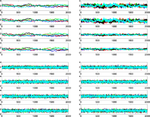
Figure 1: A simple test case where only one source parameter $z$ is allowed to vary. Top left: trace plots of location parameter $z$ at four selected timesteps (9th, 10th, 11th and 12th) by the random-walk MCMC within Gibbs. Similar plots are also shown for the hybrid MCMC within Gibbs (top right), regular SIS method with rejection (bottom left) and improved SIS method with resampling (bottom right).

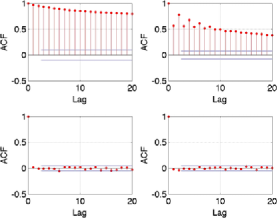
Figure 2: Autocorrelation plots for the four methods. Top left: random-walk MCMC within Gibbs; top right: hybrid MCMC within Gibbs; bottom left: SIS method with rejection; bottom right: SIS with resampling.

Simulated case 1

Before running our algorithms for a long time, we tested a simplified case where the simulation was run for only $15$ timesteps with only one of the six parameters allowed to vary. In this very simple example, the dipole only moves in the $z$ dimension in the brain and both the strength and moments of the dipole remain constant. The parameters of the simulated dipole are summarized in Table 1. The regular SIS method with rejection and the improved SIS method with resampling were tested. The random-walk MCMC within Gibbs and the hybrid MCMC within Gibbs were also run for comparison. We randomly generated 25 data sets and tested them under each scenario. Figure 1 shows the trace plots (only 5 overlay plots are shown) for 4 selected timesteps from all the methods. We observe that both the random-walk MCMC within Gibbs and hybrid MCMC within Gibbs do not provide a stable estimate for each timepoint and their samples are highly correlated. Both of our methods produce much nicer samples which oscillate around the true values. To have a quantitative comparison, we conducted a detailed convergence diagnosis for each approach: the sample autocorrelation function of the chain at a selected timestep was computed for each approach (see Figure 2); the effective sample size of the averaged chain from each approach was calculated; Gelman–Rubin’s method was used for evaluating convergence; similar methods such as Geweke, Heidelberger–Welch and Raftery–Lewis were also employed for diagnosis (see Table 2). Both Figures 1, 2 and Table 2 show strong evidence that our approaches outperform the MCMC methods.

Table 2: Convergence diagnosis by effective sample size (ESS), Gelman–Rubin (GR) [Gelman and Rubin (1992)]: value near 1 suggests convergence, Geweke (GE) [Geweke (1992)]: $z$-score for stationary test, Heidelberger–Welch (HW) [Heidelberger and Welch (1983)]: $p$ value for stationary test, Raftery–Lewis (RL) [Raftery and Lewis (1992)]: large value suggests strong autocorrelation

Method	ESS	GR	GE	HW	RL
Random-walk MCMC within Gibbs	$26.7$	$1.29$	$-14.968$	$0.05$	$18.2$
Hybrid MCMC within Gibbs	$553.5$	$1.06$	$-4.985$	$0.116$	$1.6$
Regular SIS with rejection	$1946.9$	$1.013$	$-0.64$	$0.25$	$1.0$
Improved SIS with resampling	$2000.0$	$1.005$	$-0.28$	$0.81$	$1.0$

=275pt Initial timepoint $\mathbf{m}_{\mathrm{int}}=(x,y,z,m_{1},m_{2},s)$ $(6,7,8,3,5,5)$ $\mathbf{m}_{\mathrm{com}}=(x,y,z,m_{1},m_{2},s)$ $(0,0,0,0,0,0)$ $\bolds{\rho}=\operatorname{diag}[\rho_{1},\rho_{2},\ldots,\rho_{6}]$ $\operatorname{diag}[0.65,0.7,0.75,0.8,0.85,0.9]$ Random-walk move $(x,y,z,m_{1},m_{2},s)$ Based on previous value Number of timesteps 10 Autoregressive move $(x,y,z,m_{1},m_{2},s)$ Based on previous value $\mathbf{m}_{\mathrm{com}}=(x,y,z,m_{1},m_{2},s)$ $(0,0,0,0,0,0)$ $\bolds{\rho}=\operatorname{diag}[\rho_{1},\rho_{2},\ldots,\rho_{6}]$ $\operatorname{diag}[0.65,0.7,0.75,0.8,0.85,0.9]$ Random-walk move $(x,y,z,m_{1},m_{2},s)$ Based on previous value Number of timesteps 10 $\cdots$ $\cdots$ Repeat until 100th timepoint

Table 3: Dipole simulation: the location parameters of the dipole are expressed in terms of Cartesian coordinates [$x$ (cm), $y$ (cm), $z$ (cm)], $m_{1}$ and $m_{2}$ are the dipole moment parameters. $s$ (mA) is the strength parameter of a dipole. The diagonal elements of $\bolds{\Sigma}_{1}$ and $\bolds{\Sigma}_{2}$ are 0.0625 fT² and 0.01 cm², respectively

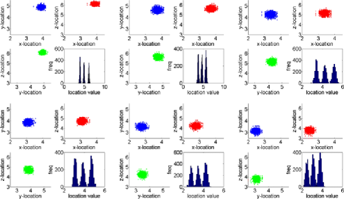
Figure 3: Source location parameters at six timesteps (a total of six $2\times 2$ subplots). Top left: in this $2\times 2$ subplot, there are three pairwise plots of the source location parameters ($x$ and $y$, $x$ and $z$, $y$ and $z$) at 1st timestep and one side by side histogram plot for the source location parameters ($x$, $y$ and $z$) at 1st timestep. The rest of the five subplots give the same information for different timesteps: 20th timestep (top middle), 40th timestep (top right), 60th timestep (bottom left), 80th timestep (bottom middle) and 100th timestep (bottom right).

Simulated case 2

In addition to case 1, a case of multiple-source parameters (three location parameters and three moment and strength parameters) was performed. In this simulation, the source was modeled as a moving dipole following a multivariate autoregressive time series. The dipole moves in the three coordinate directions $x$, $y$ and $z$, and both strength and moments of the dipole change as well. The total length of simulation is 100 timesteps (we will run 2000 timesteps for data in Section 4.3). To control the movement of the simulated dipole (to not move outside of the brain when the number of timepoints are large), we restricted the range of each parameter for the dipole. In order to do this, we set boundary values for each parameter (i.e., maximum and minimum). The autoregressive model for $\mathbf{J}^{\mathrm{P}}_{t}$ in Section 2 occurred only at certain timepoints when specified in advanced. In other words, the dipole had two types of moves: one is a move based on the autoregressive model, and the other is a random-walk move. The dipole moved according to the autoregressive model at certain specified timesteps whereas the random walk was applied to the dipole at the rest of the timepoints. We had similar restrictions on the other parameters of the dipole. The parameters setup is given in Table 3. The plots (histogram) for each dipole location parameter and pairwise plots for the location parameters are shown in Figure 3. These side by side histograms show the distribution of each location parameter at six selected timepoints. Similar plots for the other three moment and strength parameters are also shown in Figure 4. We can see that the distributions (non-Gaussian) of each parameter of the source are varying at each timestep as we expected.

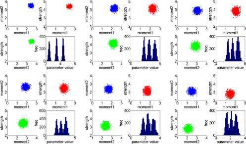
Figure 4: Source moment and strength parameters at six timesteps (a total of six $2\times 2$ subplots). Top left: in this $2\times 2$ subplot, there are three pairwise plots of the source moment and strength parameters ($m_{1}$ and $m_{2}$, $m_{1}$ and $s$ and $m_{2}$ and $s$) at 1st timestep and one side by side histogram plot for the moment and strength parameters ($m_{1}$, $m_{2}$ and $s$) at 1st timestep. The rest of the five subplots give the same information for different timesteps: 20th timestep (top middle), 40th timestep (top right), 60th timestep (bottom left), 80th timestep (bottom middle) and 100th timestep (bottom right).

4.2 Parallel virtual machine (PVM) for high dimension in time

In practice, the MEG data set we have from an experiment is very large (e.g., hundreds of thousands of timesteps). The same algorithms (Sections 3.3 and 3.4) need to be run for a much longer time. To be exact, if we run for 5000 timesteps with 1500 replications (sample paths) for each $\mathbf{J}^{\mathrm{P}}_{t}$, we are supposed to get a stream of $S_{5000}=\{(\mathcal{J}^{\mathrm{P}}_{5000})^{(j)},j=1,\ldots,1500\}$ ($S_{t}$ is defined in Section 3.2). Because of the sequential character of our algorithms, sample paths [$(\mathbf{J}^{\mathrm{P}}_{t})^{(j)},j=1,\ldots,m$] for each time are computed in a sequential fashion and the weights updated at each time. Therefore, it is very inefficient to get the sample paths for a longer time.

Note that we always need the sample path from the previous time ($\mathbf{J}^{\mathrm{P}}_{t-1}$) when we work on the current time ($\mathbf{J}^{\mathrm{P}}_{t}$) and they are not independent, therefore, it is not possible to improve the speed in the direction of time [e.g., $(\mathbf{J}^{\mathrm{P}}_{t})^{(j)}$ sequentially depends on $(\mathbf{J}^{\mathrm{P}}_{t-1})^{(j)}$]. However, the sample paths are independent within each timestep; this is to say, at time $t$, $(\mathbf{J}^{\mathrm{P}}_{t})^{(j)}$ is independent $(\mathbf{J}^{\mathrm{P}}_{t})^{(j^{\prime})}$, so they can be computed in a separate fashion. In other words, it is always possible for us to compute several sample paths (several chunks) for the same timestep (at time $t$) simultaneously. This simultaneous computation for sample paths up to the final timestep (5000) could be achieved by parallel computing where each parallel thread would contain a sequential calculation for all the time $t$ ($1\leq t\leq 5000$) with fewer samples, so that our sequential problem can be solved in parallel. The Parallel Virtual Machine (PVM) [Geist et al. (1994)], a parallel computing paradigm, is used to speed up the computation. It is designed to allow a network of heterogeneous machines to be used as a single distributed parallel processor, so that a large scale computing problem can be solved more cost effectively. The PVM structure we use is a Master–Worker model where there are several worker programs performing tasks in parallel and a master program collecting the outcomes from each worker. Each task is to separately compute a subset of the sample paths for all timesteps. The resampling scheme is included in the worker program and there is no parallelism in time. To be exact, if there are three worker programs in the Master–Worker model to generate a steam $S_{T}=\{(\mathcal{J}^{\mathrm{P}}_{T})^{(j)},j=1,\ldots,m\}$, the way of running PVM is as follows:

 (i) Initialize each worker program and let each worker run for a substream $S^{\prime}_{T}=\{(\mathcal{J}^{\mathrm{P}}_{T})^{(j)},j=1,\ldots,\frac{m}{3}\}$.

(ii) Stack each $S^{\prime}_{T}$ and get a complete $S_{T}$.

Algorithm 2 PVM schedule

The size of $S^{\prime}_{T}$ can be adjusted according to the size of $S_{T}$ and the number of worker programs that are in use. The speed is mainly influenced by hardware and software components of network and I/O systems. It also depends on the number of worker programs, for example, adding too many parallel workers does not enhance the speed when most of the time is spent on master–worker communication. In practice, deciding on the number of workers requires experience and it varies for different machines. Because the magnetic fields generated by independent dipoles add up, there is no additional complexity (other than increased computation) brought by multiple dipoles.

Since our PVM program involves randomness and a resampling scheme, several issues still need to be resolved. First, if our algorithms were implemented in a single program without parallelism, all samples generated before resampling from this program should be simply related to the random number generator. However, when there are several workers, each of them doing the same thing as a single program but in parallel, the unique randomness within each worker will eventually come up with different but similar samples before resampling. To be exact, in order to have the two programs generate the same results, in the PVM structure we need to explicitly and precisely choose different workers according to a predefined random sequence. This random sequence can be obtained from a single program without parallelism. Unfortunately, this needs a lot of work in programming and would surely slow down the computation. Second, in a single program without parallelism, we would only have one resampling procedure. The samples would be generated from the resampling procedure. However, there would be one resampling procedure within each of our worker programs in PVM. The samples would be generated from each of these workers and should eventually be pooled together. In principle, the weights from each worker should be pooled first and then we would perform the resampling procedure. The reason is that each worker might generate different weights so that the normalizing constants might be different. If the resampling happens only one time (at the end of all timesteps), a reasonable way to solve this problem is that we can do the resampling scheme in the master program after normalizing all the weights when pooled. If there were several resampling schemes before the end, we could still return to the master program when necessary. Again, this needs extensive programming and, again, it would surely slow down the computations. In our current program, sums of weights within each worker were almost the same (normalizing constants were almost the same), so we retained the resampling procedure in each worker program. Because the random number generation will not produce the same numbers in a parallel program as in a sequential program without extensive interprocess communication and because resampling within each parallel worker program will produce different results than would resampling in the master, we do not expect the identical samples in the parallel version of our sequential program. We do expect the distribution of the samples from the parallel program to be indistinguishable from the distribution of the samples from the sequential version.

4.3 Numerical results for running PVM for MEG model

The PVM was first run on a single Linux workstation (Intel Pentium 4 CPU 3.80 GHz, Memory 2 GB) for different configurations. The data size was $2000$ MEG timesteps with $1500$ sample paths for each timestep. We split the computation into a number of tasks: $1$ (without PVM), $3$, $5$, $10$ and $15$ workers, respectively, and run for $100$, $500$, $1000$, $1500$ and $2000$ timesteps. The user CPU time (total number of CPU-seconds for master and worker programs) is used to measure the time spent by each PVM run. The real time elapsed (minutes) is also shown in parentheses beside the user CPU time. The result is shown in Table 4.

Table 4: PVM application on a single workstation. Five different PVM configurations were run. The number of workers in PVM is denoted “number of tasks.” The number of sample paths within each worker is denoted “load per task.” Each PVM run eventually generates 1500 sample paths

Number	Load	Time 1	Time 2	Time 3	Time 4	Time 5
of tasks	per task	(100)	(500)	(1000)	(1500)	(2000)
1	$1500$	0.008 (1.00)	0.032 (5.12)	0.064 (10.35)	0.120 (16.47)	0.136 (22.08)
3	$500$	0.008 (0.24)	0.032 (2.05)	0.060 (4.12)0	0.096 (6.23)0	0.148 (8.40)0
5	$300$	0.008 (0.17)	0.036 (1.27)	0.064 (3.17)0	0.104 (4.25)0	0.148 (6.47)0
10	$150$	0.008 (0.11)	0.040 (0.59)	0.072 (1.59)0	0.096 (3.00)0	0.136 (4.51)0
15	$100$	0.008 (0.10)	0.036 (0.50)	0.064 (1.43)0	0.124 (2.33)0	0.164 (3.24)0

We can see that the user CPU time increases roughly linearly in the number of timesteps from $0.008$ second to $0.146$ second on average. The linear relationship of user CPU time on experiment time is almost the same for each of these PVM configurations as we expected. This can be clearly observed from Figure 5: in Figure 5(a), these lines (user CPU time/Task) are nearly equally distant and stay roughly constant for different tasks within the samesteps time run; in Figure 5(b), the slope of each line (user CPU time/Timesteps) is almost the same. Note that there is a significant difference in real time elapsed for different PVM configurations. This should not be considered a contradiction with user CPU time because real time elapsed is mostly affected by other programs and it includes time spent in memory, I/O and other resources.

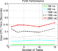
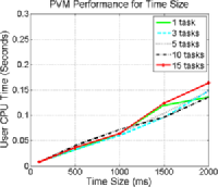
(a) CPU time with tasks	(b) CPU time with timesteps

Figure 5: PVM Performance: user CPU time (seconds) for number of tasks and different time run. (a) Each line (with a specific timestep) is a plot of user CPU time for different number of tasks. (b) Each line (with a specific number of tasks) is a plot of user CPU time for different timesteps.

Table 5: PVM application on multiple workstations. This table shows the user CPU time (seconds) for each PVM run and real time elapsed (minutes) in parentheses using one, two, three and four machines. The length of each PVM run was 1500 timesteps

Number	Load	Time 1	Time 2	Time 3	Time 4
of tasks	per task	(1500)	(1500)	(1500)	(1500)
3	500	0.084 (7.56)	0.128 (5.46)	0.108 (3.39)	0.096 (2.34)
5	300	0.100 (4.55)	0.084 (3.10)	0.124 (2.23)	0.108 (1.29)
10	150	0.100 (3.19)	0.096 (1.51)	0.104 (1.39)	0.116 (1.03)
15	100	0.124 (2.34)	0.112 (1.31)	0.104 (1.00)	0.112 (0.44)

The performance can still be improved when extra machines are included. Table 5 lists the PVM performance of 1–4 machines with $1500$ timesteps. First, since user CPU time is the sum of the CPU time for master and worker programs, it is expected that the user CPU time for each of these PVM runs is roughly $0.120$ second. Second, the real elapsed time of each PVM run is cut to 50%–70% if one machine is added. It then goes down to 40%–50% when three computers are employed. The real time elapsed decreases to 10%–30% when four computers are added. These performances are based on our public cluster with heterogeneous CPU speed and cache size. The theoretical reduction in execution time of PVM is not necessarily achieved. Finally, to get better time execution by PVM, we suggest to adjust the number of CPUs and the number of tasks, and to use relatively similar machines. To summarize, Figure 6 is a graphic illustration of both real time elapsed and user CPU time for our PVM run.

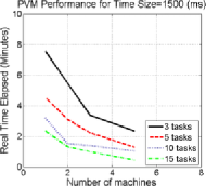
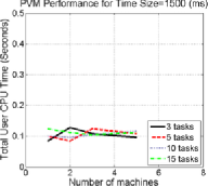
(a) Real time for PVM run	(b) Total user CPU time for PVM run

Figure 6: PVM Performance: real time elapsed (minutes) and user CPU time (seconds) graph for number of machines for 1500 timesteps PVM run. (a) Each line (with a specific number of tasks) is a plot of real time elapsed for a different number of machines. (b) Each line (with a specific number of tasks) is a plot of total user CPU time of master and worker programs for different number of machines.

5 A real data application

Data was collected by a 306-channel system (Elekta-Neuromag) at the Center for Advanced Brain Magnetic Source Imaging (CABMSI) at UPMC Presbyterian Hospital in Pittsburgh in an experiment related to Brain-controlled interfaces (BCI). A BCI expresses motor commands via neural signals directly from the brain. The experiment involves two parts (see Figure 7): in the first part the subjects were asked to imagine performing the “center-out” task using the wrist (imagined movement task) and in the second part the subjects controlled a 2-D cursor using the wrist to perform the center-out task following a visual target (overt movement task).

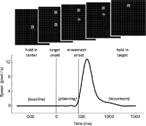
Figure 7: The subject controls the 2-D cursor position using wrist movements. The cursor needs to go to the center and stay there for a hold period until the peripheral target appears. Then the cursor moves from the center out to the target and stays there for another hold period to complete the trial successfully. The target changes color when hit by the cursor and disappears when the holding period has finished. The bottom trace shows the speed profile of the cursor from a representative trial, and the dotted lines delimit the pre-movement/planning period. Figure and explanation were obtained from Wang et al. (2010).

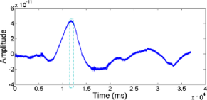
Figure 8: The MEG signal of a typical trial at a magnetometer. The horizontal axis is time (ms) and the vertical axis is the magnitude of the signal (fT).

The data consists of one trial recording 37,000 milliseconds at 102 MEG sensors (magnetometers). We used this data for testing our model along with our PVM scheme. Instead of analyzing the whole trial of data, we only analyzed about 400 milliseconds (dashed box in Figure 8) after movement onset (12,000 milliseconds–12,400 milliseconds in the original data) from all the channels. To simplify our calculation for the real data, we were only estimating the location of the source $(x,y,z)$. The moment and strength parameters $(m_{1},m_{2},s)$ were not of our interest (not varying too much by assumption). The choice of prior for real data is an open question; we used almost the same prior as we did in Section 4 for simplification. We set the mean $\mathbf{m}_{\mathrm{ini}}$ of the initial state $\mathbf{J}^{\mathrm{P}}_{0}$ as $(-4,-4,11)$ motivated by the minimum norm estimate [Hämäläinen and Ilmoniemi (1994)], which is $(-2,-2,10)$. We further assumed a unit moment and strength for the dipole in the data. The starting values for the initial state $(x,y,z,m_{1},m_{2},s)$ were set to $(-4.06,-3.77,13.13,1.11,0.98,1.12)$. The empirical density plots of the dipole location parameter ($x$, $y$, $z$) at two selected timesteps are shown in Figure 9. Using the density plots of the location parameters, we were able to find the dipole distribution at different timesteps. Figure 10 shows several snapshots of dipole distribution at six timesteps, that is, the data cloud in each plot tells where the dipole might be located at a given timestep. A full movie of the dipole distribution for 100 milliseconds can be found at http://smat.epfl.ch/~zyao/3dplot_animation.gif. Different initial values might have different performance due to the complexity of the problem and the real data, thus, a more realistic prior needs to be investigated in our future work. We ran PVM for 1500 milliseconds (12,000 milliseconds–13,500 milliseconds in the original data) with the same PVM configuration as our simulation; the time spent was very close to that from our previous simulation results.

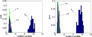
Figure 9: Empirical density for source location parameter ($x$, $y$, $z$). Left: density plot for $1$st millisecond; right: density plot for $101$st millisecond.

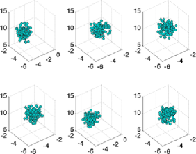
Figure 10: Time variation of the dipole distribution. Upper row: dipole distribution at $1$st, $21$st and $41$st millisecond (left to right); lower row: dipole distribution at $61$st, $81$st and $101$st millisecond.

A typical MEG analysis would report the estimated movement of the dipole at each time step. We can do the same. Additionally, because we have samples from a probability distribution we can provide estimates of the variation of the estimated movement and other source parameters. Other methods cannot provide appropriate estimates of variation. In clinical applications, estimates of variation may provide neurosurgeons a much better basis for their decisions. We still need to overcome the computational burden to make our method feasible for a complete application.

6 Conclusion and discussion

We have introduced a general state-space formulation for the time dependency of the parameters of a current dipole which generates the MEG signals. In this paper we have only considered the simplest sort of model, a first order autoregression for the time dependency. However, the framework allows for much more complex models. And, because three of the parameters are spatial coordinates, the model automatically incorporates space–time dependencies. The time dependency in the model has greatly expanded the parameter space. That fact together with the nonlinearity of the model means that more typical MCMC methods converge extremely slowly. The benefit of sequential methods is that we do not attempt to estimate the entire target distribution at once but rather attempt to estimate samples for each time point sequentially. Because of the expanded parameter space, the need for parallel computational methods is obvious. Our initial attempt utilized PVM and provided the expected reduction in running time.

The results so far are mainly based on a one-source model where we assumed there was only one dipole in the data. The extension from one source to multiple sources is natural and only the computational complexity increases. Our algorithms will still work in this multiple-source model case. However, to determine the number of sources in the MEG data is still an open question. In general, there are three ways of finding the number of sources for the advanced model. The first one, which is relatively easy, is to use a predefined number of sources for the data. The second one is to estimate the number of sources from the data in advance [Waldorp et al. (2005), Bai and He (2006), Yao and Eddy (2012)]. The third one is to model the number of the sources using a prior distribution [Bertrand et al. (2001)].

We fixed several parameters when we compared our algorithms with other MCMC methods. In fact, those parameters could be estimated along with the source distribution. The natural way of implementing this is to include the estimation of those parameters and the source distribution in the iterations until all of them become stable. Furthermore, the skewness of weights that arises in sequential importance sampling could be a trade-off between the efficiency of the algorithm and the quality of the source distribution. Naturally, we have observed some skewness in the weights; we do not have enough experience to evaluate whether this skewness should be considered excessive or unusual. Residual sampling [Liu and Chen (1998)] or stratified sampling [Kitagawa (1996)] could replace regular weight sampling and might address excessive skewness.

To summarize, due to its nonuniqueness, finding a good estimate of the MEG source is a challenging problem which is still open. We have proposed a predictive model for finding a distribution for the MEG source and we have applied our methods on both simulated data and real data. In practice, the MEG data sets from different experimental settings are much more complicated. Our methods can be used as a reference with other source localization methods. Driven by the desire of looking at the brain activity in real time, we plan to implement a computing environment to study the brain activity under the real MEG temporal resolution ($1/1000$ sec). The computational challenge arises due to the extremely large dimensionality of the problem (high resolution); there is no common computing architecture that could help. We are exploring the use of more advanced forms of parallelism such as CUDA (Compute Unified Device Architecture) and OPENCL to further reduce the running time in the future.

References

- Andrieu and Thoms (2008) {barticle}[mr] \bauthor\bsnmAndrieu, \bfnmChristophe\binitsC. and \bauthor\bsnmThoms, \bfnmJohannes\binitsJ. (\byear2008). \btitleA tutorial on adaptive MCMC. \bjournalStat. Comput. \bvolume18 \bpages343–373. \biddoi=10.1007/s11222-008-9110-y, issn=0960-3174, mr=2461882 \bptokimsref\endbibitem
- Bai and He (2006) {barticle}[author] \bauthor\bsnmBai, \bfnmXiaoxiao\binitsX. and \bauthor\bsnmHe, \bfnmBin\binitsB. (\byear2006). \btitleEstimation of number of independent brain electric sources from the scalp EEGs. \bjournalIEEE Trans. Biomed. Eng. \bvolume53 \bpages1883–1892. \bptokimsref\endbibitem
- Barkley and Baumgartner (2003) {barticle}[pbm] \bauthor\bsnmBarkley, \bfnmGregory L.\binitsG. L. and \bauthor\bsnmBaumgartner, \bfnmChristoph\binitsC. (\byear2003). \btitleMEG and EEG in epilepsy. \bjournalJ. Clin. Neurophysiol. \bvolume20 \bpages163–178. \bidissn=0736-0258, pmid=12881663 \bptokimsref\endbibitem
- Bertrand et al. (2001) {barticle}[pbm] \bauthor\bsnmBertrand, \bfnmC.\binitsC., \bauthor\bsnmOhmi, \bfnmM.\binitsM., \bauthor\bsnmSuzuki, \bfnmR.\binitsR. and \bauthor\bsnmKado, \bfnmH.\binitsH. (\byear2001). \btitleA probabilistic solution to the MEG inverse problem via MCMC methods: The reversible jump and parallel tempering algorithms. \bjournalIEEE Trans. Biomed. Eng. \bvolume48 \bpages533–542. \biddoi=10.1109/10.918592, issn=0018-9294, pmid=11341527 \bptokimsref\endbibitem
- Berzuini et al. (1997) {barticle}[mr] \bauthor\bsnmBerzuini, \bfnmCarlo\binitsC., \bauthor\bsnmBest, \bfnmNicola G.\binitsN. G., \bauthor\bsnmGilks, \bfnmWalter R.\binitsW. R. and \bauthor\bsnmLarizza, \bfnmCristiana\binitsC. (\byear1997). \btitleDynamic conditional independence models and Markov chain Monte Carlo methods. \bjournalJ. Amer. Statist. Assoc. \bvolume92 \bpages1403–1412. \biddoi=10.2307/2965410, issn=0162-1459, mr=1615251 \bptokimsref\endbibitem
- Campi et al. (2008) {barticle}[auto:STB—2014/05/28—10:36:42] \bauthor\bsnmCampi, \bfnmC.\binitsC., \bauthor\bsnmPascarella, \bfnmA.\binitsA., \bauthor\bsnmSorrentino, \bfnmA.\binitsA. and \bauthor\bsnmPiana, \bfnmM.\binitsM. (\byear2008). \btitleA Rao–Blackwellized particle filter for magnetoencephalography. \bjournalInverse Problems \bvolume24 \bpages25023–25037. \bptokimsref\endbibitem
- Campi et al. (2011) {bmisc}[auto:STB—2014/05/28—10:36:42] \bauthor\bsnmCampi, \bfnmC.\binitsC., \bauthor\bsnmPascarella, \bfnmA.\binitsA., \bauthor\bsnmSorrentino, \bfnmA.\binitsA. and \bauthor\bsnmPiana, \bfnmM.\binitsM. (\byear2011). \bhowpublishedHighly automated dipole estimation. Computational Intelligence and Neuroscience 2011 Article ID 982185, 11 pp. \bptokimsref\endbibitem
- Carlin, Polson and Stoffer (1992) {barticle}[author] \bauthor\bsnmCarlin, \bfnmB. P.\binitsB. P., \bauthor\bsnmPolson, \bfnmN. G.\binitsN. G. and \bauthor\bsnmStoffer, \bfnmD. S.\binitsD. S. (\byear1992). \btitleA Monte Carlo approach to nonnormal and nonlinear state-space modeling. \bjournalJ. Amer. Statist. Assoc. \bvolume87 \bpages493–500. \bptokimsref\endbibitem
- Carter and Kohn (1994) {barticle}[mr] \bauthor\bsnmCarter, \bfnmC. K.\binitsC. K. and \bauthor\bsnmKohn, \bfnmR.\binitsR. (\byear1994). \btitleOn Gibbs sampling for state space models. \bjournalBiometrika \bvolume81 \bpages541–553. \biddoi=10.1093/biomet/81.3.541, issn=0006-3444, mr=1311096 \bptokimsref\endbibitem
- Cohen (1968) {barticle}[pbm] \bauthor\bsnmCohen, \bfnmD.\binitsD. (\byear1968). \btitleMagnetoencephalography: Evidence of magnetic fields produced by alpha-rhythm currents. \bjournalScience \bvolume161 \bpages784–786. \bidissn=0036-8075, pmid=5663803 \bptokimsref\endbibitem
- Del Moral, Doucet and Jasra (2006) {barticle}[mr] \bauthor\bparticleDel \bsnmMoral, \bfnmPierre\binitsP., \bauthor\bsnmDoucet, \bfnmArnaud\binitsA. and \bauthor\bsnmJasra, \bfnmAjay\binitsA. (\byear2006). \btitleSequential Monte Carlo samplers. \bjournalJ. R. Stat. Soc. Ser. B Stat. Methodol. \bvolume68 \bpages411–436. \biddoi=10.1111/j.1467-9868.2006.00553.x, issn=1369-7412, mr=2278333 \bptokimsref\endbibitem
- Fearnhead (2008) {barticle}[mr] \bauthor\bsnmFearnhead, \bfnmPaul\binitsP. (\byear2008). \btitleComputational methods for complex stochastic systems: A review of some alternatives to MCMC. \bjournalStat. Comput. \bvolume18 \bpages151–171. \biddoi=10.1007/s11222-007-9045-8, issn=0960-3174, mr=2390816 \bptokimsref\endbibitem
- Gamerman (1998) {barticle}[mr] \bauthor\bsnmGamerman, \bfnmDani\binitsD. (\byear1998). \btitleMarkov chain Monte Carlo for dynamic generalised linear models. \bjournalBiometrika \bvolume85 \bpages215–227. \biddoi=10.1093/biomet/85.1.215, issn=0006-3444, mr=1627273 \bptokimsref\endbibitem
- Geist et al. (1994) {bbook}[author] \bauthor\bsnmGeist, \bfnmAl\binitsA., \bauthor\bsnmBeguelin, \bfnmAdam\binitsA., \bauthor\bsnmDongarra, \bfnmJack\binitsJ., \bauthor\bsnmJiang, \bfnmWeicheng\binitsW., \bauthor\bsnmManchek, \bfnmRobert\binitsR. and \bauthor\bsnmSunderam, \bfnmVaidyalingam S.\binitsV. S. (\byear1994). \btitlePVM: Parallel Virtual Machine: A Users’ Guide and Tutorial for Network Parallel Computing (Scientific and Engineering Computation). \bpublisherMIT Press, \blocationCambridge, MA. \bptokimsref\endbibitem
- Gelman, Roberts and Gilks (1996) {bincollection}[mr] \bauthor\bsnmGelman, \bfnmA.\binitsA., \bauthor\bsnmRoberts, \bfnmG. O.\binitsG. O. and \bauthor\bsnmGilks, \bfnmW. R.\binitsW. R. (\byear1996). \btitleEfficient Metropolis jumping rules. In \bbooktitleBayesian Statistics \bpages599–607. \bpublisherOxford Univ. Press, \blocationNew York. \bidmr=1425429 \bptokimsref\endbibitem
- Gelman and Rubin (1992) {barticle}[author] \bauthor\bsnmGelman, \bfnmAndrew\binitsA. and \bauthor\bsnmRubin, \bfnmDonald B.\binitsD. B. (\byear1992). \btitleInference from iterative simulation using multiple sequences. \bjournalStatist. Sci. \bvolume7 \bpages457–511. \bptokimsref\endbibitem
- Geweke (1992) {bincollection}[mr] \bauthor\bsnmGeweke, \bfnmJohn\binitsJ. (\byear1992). \btitleEvaluating the accuracy of sampling-based approaches to the calculation of posterior moments. In \bbooktitleBayesian Statistics \bpages169–193. \bpublisherOxford Univ. Press, \blocationNew York. \bidmr=1380276 \bptokimsref\endbibitem
- Gordon, Salmond and Smith (1993) {barticle}[author] \bauthor\bsnmGordon, \bfnmN. J.\binitsN. J., \bauthor\bsnmSalmond, \bfnmD. J.\binitsD. J. and \bauthor\bsnmSmith, \bfnmA. F. M.\binitsA. F. M. (\byear1993). \btitleNovel approach to nonlinear/non-Gaussian Bayesian state estimation. \bjournalIEE Proceedings F (Radar and Signal Processing) \bvolume140 \bpages107–113. \bptokimsref\endbibitem
- Griffiths (1999) {bbook}[author] \bauthor\bsnmGriffiths, \bfnmDavid J.\binitsD. J. (\byear1999). \btitleIntroduction to Electrodynamics. \bpublisherPrentice Hall, \blocationNew York. \bptokimsref\endbibitem
- Hämäläinen and Ilmoniemi (1994) {barticle}[pbm] \bauthor\bsnmHämäläinen, \bfnmM. S.\binitsM. S. and \bauthor\bsnmIlmoniemi, \bfnmR. J.\binitsR. J. (\byear1994). \btitleInterpreting magnetic fields of the brain: Minimum norm estimates. \bjournalMed. Biol. Eng. Comput. \bvolume32 \bpages35–42. \bidissn=0140-0118, pmid=8182960 \bptokimsref\endbibitem
- Hämäläinen et al. (1993) {barticle}[author] \bauthor\bsnmHämäläinen, \bfnmM. S.\binitsM. S., \bauthor\bsnmHari, \bfnmR.\binitsR., \bauthor\bsnmIlmoniemi, \bfnmR. J.\binitsR. J., \bauthor\bsnmKnuutila, \bfnmJ.\binitsJ. and \bauthor\bsnmLounasmaa, \bfnmO. V.\binitsO. V. (\byear1993). \btitleMagnetoencephalography—theory, instrumentation, and applications to noninvasive studies of signal processing in the human brain. \bjournalRev. Modern Phys. \bvolume65 \bpages413–497. \bptokimsref\endbibitem
- Heidelberger and Welch (1983) {barticle}[author] \bauthor\bsnmHeidelberger, \bfnmPhilip\binitsP. and \bauthor\bsnmWelch, \bfnmPeter D.\binitsP. D. (\byear1983). \btitleSimulation run length control in the presence of an initial transient. \bjournalOper. Res. \bvolume31 \bpages1109–1144. \bptokimsref\endbibitem
- Jun et al. (2005) {barticle}[pbm] \bauthor\bsnmJun, \bfnmSung C.\binitsS. C., \bauthor\bsnmGeorge, \bfnmJohn S.\binitsJ. S., \bauthor\bsnmParé-Blagoev, \bfnmJuliana\binitsJ., \bauthor\bsnmPlis, \bfnmSergey M.\binitsS. M., \bauthor\bsnmRanken, \bfnmDoug M.\binitsD. M., \bauthor\bsnmSchmidt, \bfnmDavid M.\binitsD. M. and \bauthor\bsnmWood, \bfnmC. C.\binitsC. C. (\byear2005). \btitleSpatiotemporal Bayesian inference dipole analysis for MEG neuroimaging data. \bjournalNeuroImage \bvolume28 \bpages84–98. \biddoi=10.1016/j.neuroimage.2005.06.003, issn=1053-8119, pii=S1053-8119(05)00400-3, pmid=16023866 \bptokimsref\endbibitem
- Kitagawa (1996) {barticle}[mr] \bauthor\bsnmKitagawa, \bfnmGenshiro\binitsG. (\byear1996). \btitleMonte Carlo filter and smoother for non-Gaussian nonlinear state space models. \bjournalJ. Comput. Graph. Statist. \bvolume5 \bpages1–25. \biddoi=10.2307/1390750, issn=1061-8600, mr=1380850 \bptokimsref\endbibitem
- Knorr-Held (1999) {barticle}[author] \bauthor\bsnmKnorr-Held, \bfnmLeonhard\binitsL. (\byear1999). \btitleConditional prior proposals in dynamic models. \bjournalScand. J. Stat. \bvolume26 \bpages129–144. \bptokimsref\endbibitem
- Kristeva-Feige et al. (1997) {barticle}[author] \bauthor\bsnmKristeva-Feige, \bfnmR.\binitsR., \bauthor\bsnmRossi, \bfnmS.\binitsS., \bauthor\bsnmFeige, \bfnmB.\binitsB., \bauthor\bsnmMergner, \bfnmTh.\binitsTh., \bauthor\bsnmLucking, \bfnmC. H.\binitsC. H. and \bauthor\bsnmRossini, \bfnmP. M.\binitsP. M. (\byear1997). \btitleThe bereitschaftspotential paradigm in investigating voluntary movement organization in humans using magnetoencephalography (MEG). \bjournalBrain Res. Protoc. \bvolume1 \bpages13–22. \bptokimsref\endbibitem
- Kybic et al. (2006) {barticle}[pbm] \bauthor\bsnmKybic, \bfnmJan\binitsJ., \bauthor\bsnmClerc, \bfnmMaureen\binitsM., \bauthor\bsnmFaugeras, \bfnmOlivier\binitsO., \bauthor\bsnmKeriven, \bfnmRenaud\binitsR. and \bauthor\bsnmPapadopoulo, \bfnmThéo\binitsT. (\byear2006). \btitleGeneralized head models for MEG/EEG: Boundary element method beyond nested volumes. \bjournalPhys. Med. Biol. \bvolume51 \bpages1333–1346. \biddoi=10.1088/0031-9155/51/5/021, issn=0031-9155, pii=S0031-9155(06)02724-2, pmid=16481698 \bptokimsref\endbibitem
- Liu (1996) {barticle}[author] \bauthor\bsnmLiu, \bfnmJ. S.\binitsJ. S. (\byear1996). \btitleMetropolized independent sampling with comparisons to rejection sampling and importance sampling. \bjournalStatist. Comput. \bvolume6 \bpages113–119. \bptokimsref\endbibitem
- Liu and Chen (1998) {barticle}[mr] \bauthor\bsnmLiu, \bfnmJun S.\binitsJ. S. and \bauthor\bsnmChen, \bfnmRong\binitsR. (\byear1998). \btitleSequential Monte Carlo methods for dynamic systems. \bjournalJ. Amer. Statist. Assoc. \bvolume93 \bpages1032–1044. \biddoi=10.2307/2669847, issn=0162-1459, mr=1649198 \bptokimsref\endbibitem
- Mattout et al. (2006) {barticle}[pbm] \bauthor\bsnmMattout, \bfnmJérémie\binitsJ., \bauthor\bsnmPhillips, \bfnmChristophe\binitsC., \bauthor\bsnmPenny, \bfnmWilliam D.\binitsW. D., \bauthor\bsnmRugg, \bfnmMichael D.\binitsM. D. and \bauthor\bsnmFriston, \bfnmKarl J.\binitsK. J. (\byear2006). \btitleMEG source localization under multiple constraints: An extended Bayesian framework. \bjournalNeuroImage \bvolume30 \bpages753–767. \biddoi=10.1016/j.neuroimage.2005.10.037, issn=1053-8119, pii=S1053-8119(05)02418-3, pmid=16368248 \bptokimsref\endbibitem
- Miao et al. (2013) {barticle}[auto:STB—2014/05/28—10:36:42] \bauthor\bsnmMiao, \bfnmL.\binitsL., \bauthor\bsnmMichael, \bfnmS.\binitsS., \bauthor\bsnmKovvali, \bfnmN.\binitsN., \bauthor\bsnmChakrabarti, \bfnmC.\binitsC. and \bauthor\bsnmPapandreou-Suppappola, \bfnmA.\binitsA. (\byear2013). \btitleMulti-source neural activity estimation and sensor scheduling: Algorithms and hardware implementation. \bjournalJournal of Signal Processing Systems \bvolume70 \bpages145–162. \bptokimsref\endbibitem
- Mosher, Lewis and Leahy (1992) {barticle}[pbm] \bauthor\bsnmMosher, \bfnmJ. C.\binitsJ. C., \bauthor\bsnmLewis, \bfnmP. S.\binitsP. S. and \bauthor\bsnmLeahy, \bfnmR. M.\binitsR. M. (\byear1992). \btitleMultiple dipole modeling and localization from spatio-temporal MEG data. \bjournalIEEE Trans. Biomed. Eng. \bvolume39 \bpages541–557. \biddoi=10.1109/10.141192, issn=0018-9294, pmid=1601435 \bptokimsref\endbibitem
- Neal (2001) {barticle}[mr] \bauthor\bsnmNeal, \bfnmRadford M.\binitsR. M. (\byear2001). \btitleAnnealed importance sampling. \bjournalStat. Comput. \bvolume11 \bpages125–139. \biddoi=10.1023/A:1008923215028, issn=0960-3174, mr=1837132 \bptokimsref\endbibitem
- Okada, Lähteenmäki and Xu (1999) {barticle}[pbm] \bauthor\bsnmOkada, \bfnmY.\binitsY., \bauthor\bsnmLähteenmäki, \bfnmA.\binitsA. and \bauthor\bsnmXu, \bfnmC.\binitsC. (\byear1999). \btitleComparison of MEG and EEG on the basis of somatic evoked responses elicited by stimulation of the snout in the juvenile swine. \bjournalClin. Neurophysiol. \bvolume110 \bpages214–229. \bidissn=1388-2457, pii=S0013-4694(98)00111-4, pmid=10210611 \bptokimsref\endbibitem
- Ou, Hämäläinen and Golland (2009) {barticle}[pbm] \bauthor\bsnmOu, \bfnmWanmei\binitsW., \bauthor\bsnmHämäläinen, \bfnmMatti S.\binitsM. S. and \bauthor\bsnmGolland, \bfnmPolina\binitsP. (\byear2009). \btitleA distributed spatio-temporal EEG/MEG inverse solver. \bjournalNeuroImage \bvolume44 \bpages932–946. \biddoi=10.1016/j.neuroimage.2008.05.063, issn=1095-9572, mid=NIHMS90513, pii=S1053-8119(08)00715-5, pmcid=2730457, pmid=18603008 \bptokimsref\endbibitem
- Raftery and Lewis (1992) {barticle}[author] \bauthor\bsnmRaftery, \bfnmA. E.\binitsA. E. and \bauthor\bsnmLewis, \bfnmS. M.\binitsS. M. (\byear1992). \btitleOne long run with diagnostics: Implementation strategies for Markov chain Monte Carlo. \bjournalStatist. Sci. \bvolume7 \bpages493–497. \bptokimsref\endbibitem
- Roberts and Rosenthal (2009) {barticle}[mr] \bauthor\bsnmRoberts, \bfnmGareth O.\binitsG. O. and \bauthor\bsnmRosenthal, \bfnmJeffrey S.\binitsJ. S. (\byear2009). \btitleExamples of adaptive MCMC. \bjournalJ. Comput. Graph. Statist. \bvolume18 \bpages349–367. \biddoi=10.1198/jcgs.2009.06134, issn=1061-8600, mr=2749836 \bptokimsref\endbibitem
- Sarvas (1984) {barticle}[author] \bauthor\bsnmSarvas, \bfnmJ.\binitsJ. (\byear1984). \btitleBasic mathematical and electromagnetic concepts of the biomagnetic inverse problem. \bjournalPhys. Med. Biol. \bvolume32 \bpages11–22. \bptokimsref\endbibitem
- Schmidt, George and Wood (1999) {barticle}[author] \bauthor\bsnmSchmidt, \bfnmD. M.\binitsD. M., \bauthor\bsnmGeorge, \bfnmJ. S.\binitsJ. S. and \bauthor\bsnmWood, \bfnmC. C.\binitsC. C. (\byear1999). \btitleBayesian inference applied to the electromagnet inverse problem. \bjournalHum. Brain Mapp. \bvolume7 \bpages195–212. \bptokimsref\endbibitem
- Shephard and Pitt (1997) {barticle}[mr] \bauthor\bsnmShephard, \bfnmNeil\binitsN. and \bauthor\bsnmPitt, \bfnmMichael K.\binitsM. K. (\byear1997). \btitleLikelihood analysis of non-Gaussian measurement time series. \bjournalBiometrika \bvolume84 \bpages653–667. \biddoi=10.1093/biomet/84.3.653, issn=0006-3444, mr=1603940 \bptokimsref\endbibitem
- Somersalo, Voutilainen and Kaipio (2003) {barticle}[mr] \bauthor\bsnmSomersalo, \bfnmE.\binitsE., \bauthor\bsnmVoutilainen, \bfnmA.\binitsA. and \bauthor\bsnmKaipio, \bfnmJ. P.\binitsJ. P. (\byear2003). \btitleNon-stationary magnetoencephalography by Bayesian filtering of dipole models. \bjournalInverse Problems \bvolume19 \bpages1047–1063. \biddoi=10.1088/0266-5611/19/5/304, issn=0266-5611, mr=2024688 \bptokimsref\endbibitem
- Sorrentino et al. (2009) {barticle}[pbm] \bauthor\bsnmSorrentino, \bfnmAlberto\binitsA., \bauthor\bsnmParkkonen, \bfnmLauri\binitsL., \bauthor\bsnmPascarella, \bfnmAnnalisa\binitsA., \bauthor\bsnmCampi, \bfnmCristina\binitsC. and \bauthor\bsnmPiana, \bfnmMichele\binitsM. (\byear2009). \btitleDynamical MEG source modeling with multi-target Bayesian filtering. \bjournalHum. Brain Mapp. \bvolume30 \bpages1911–1921. \biddoi=10.1002/hbm.20786, issn=1097-0193, pmid=19378276 \bptokimsref\endbibitem
- Sorrentino et al. (2013) {barticle}[mr] \bauthor\bsnmSorrentino, \bfnmAlberto\binitsA., \bauthor\bsnmJohansen, \bfnmAdam M.\binitsA. M., \bauthor\bsnmAston, \bfnmJohn A. D.\binitsJ. A. D., \bauthor\bsnmNichols, \bfnmThomas E.\binitsT. E. and \bauthor\bsnmKendall, \bfnmWilfrid S.\binitsW. S. (\byear2013). \btitleDynamic filtering of static dipoles in magnetoencephalography. \bjournalAnn. Appl. Stat. \bvolume7 \bpages955–988. \bidissn=1932-6157, mr=3113497 \bptokimsref\endbibitem
- Srinivasan (2002) {bbook}[mr] \bauthor\bsnmSrinivasan, \bfnmRajan\binitsR. (\byear2002). \btitleImportance Sampling: Applications in Communications and Detection. \bpublisherSpringer, \blocationBerlin. \bidmr=1949250 \bptokimsref\endbibitem
- Uutela, Hämäläinen and Somersalo (1999) {barticle}[author] \bauthor\bsnmUutela, \bfnmK.\binitsK., \bauthor\bsnmHämäläinen, \bfnmM. S.\binitsM. S. and \bauthor\bsnmSomersalo, \bfnmE.\binitsE. (\byear1999). \btitleVisualization of magnetoencephalographic data using minimum current estimates. \bjournalNeuroImage \bvolume10 \bpages173–180. \bptokimsref\endbibitem
- Van Veen, Joseph and Hecox (1992) {binproceedings}[author] \bauthor\bparticleVan \bsnmVeen, \bfnmB.\binitsB., \bauthor\bsnmJoseph, \bfnmJ.\binitsJ. and \bauthor\bsnmHecox, \bfnmK.\binitsK. (\byear1992). \btitleLocalization of intra-cerebral sources of electrical activity via linearly constrained minimum variance spatial filtering. In \bbooktitleProc. IEEE 6th SP Workshop on Statistical Signal and Array Processing \bpages526–529. \blocationVictoria, BC. \bptokimsref\endbibitem
- Waldorp et al. (2005) {barticle}[pbm] \bauthor\bsnmWaldorp, \bfnmLourens J.\binitsL. J., \bauthor\bsnmHuizenga, \bfnmHilde M.\binitsH. M., \bauthor\bsnmNehorai, \bfnmArye\binitsA., \bauthor\bsnmGrasman, \bfnmRaoul P. P P.\binitsR. P. P. P. and \bauthor\bsnmMolenaar, \bfnmPeter C. M.\binitsP. C. M. (\byear2005). \btitleModel selection in spatio-temporal electromagnetic source analysis. \bjournalIEEE Trans. Biomed. Eng. \bvolume52 \bpages414–420. \biddoi=10.1109/TBME.2004.842982, issn=0018-9294, pmid=15759571 \bptokimsref\endbibitem
- Wang et al. (2010) {barticle}[pbm] \bauthor\bsnmWang, \bfnmWei\binitsW., \bauthor\bsnmSudre, \bfnmGustavo P.\binitsG. P., \bauthor\bsnmXu, \bfnmYang\binitsY., \bauthor\bsnmKass, \bfnmRobert E.\binitsR. E., \bauthor\bsnmCollinger, \bfnmJennifer L.\binitsJ. L., \bauthor\bsnmDegenhart, \bfnmAlan D.\binitsA. D., \bauthor\bsnmBagic, \bfnmAnto I.\binitsA. I. and \bauthor\bsnmWeber, \bfnmDouglas J.\binitsD. J. (\byear2010). \btitleDecoding and cortical source localization for intended movement direction with MEG. \bjournalJ. Neurophysiol. \bvolume104 \bpages2451–2461. \biddoi=10.1152/jn.00239.2010, issn=1522-1598, pii=jn.00239.2010, pmcid=2997025, pmid=20739599 \bptokimsref\endbibitem
- Yao and Eddy (2012) {bmisc}[author] \bauthor\bsnmYao, \bfnmZhigang\binitsZ. and \bauthor\bsnmEddy, \bfnmWilliam F.\binitsW. F. (\byear2012). \bhowpublishedStatistical approaches to estimating the number of signal sources in magnetoencephalography. Unpublished manuscript. \bptokimsref\endbibitem