Robust error bounds for finite element approximation of reaction-diffusion problems with non-constant reaction coefficient in arbitrary space dimension

Abstract.

We present a fully computable a posteriori error estimator for piecewise linear finite element approximations of reaction-diffusion problems with mixed boundary conditions and piecewise constant reaction coefficient formulated in arbitrary dimension. The estimator provides a guaranteed upper bound on the energy norm of the error and it is robust for all values of the reaction coefficient, including the singularly perturbed case. The approach is based on robustly equilibrated boundary flux functions of Ainsworth and Oden (Wiley 2000) and on subsequent robust and explicit flux reconstruction. This paper simplifies and extends the applicability of the previous result of Ainsworth and Vejchodský (Numer. Math. 119 (2011) 219–243) in three aspects: (i) arbitrary dimension, (ii) mixed boundary conditions, and (iii) non-constant reaction coefficient. It is the first robust upper bound on the error with these properties. An auxiliary result that is of independent interest is the derivation of new explicit constants for two types of trace inequalities on simplices.

1. Introduction

Consider a linear reaction-diffusion problem in a domain $\Omega\subset\mathbb{R}^{d}$ with mixed boundary conditions:

$$-\Delta u+\kappa^{2}u=f\quad\text{in }\Omega;\qquad u=0\quad\text{on }{\Gamma_{\mathrm{D}}};\qquad\partial u/\partial\boldsymbol{n}=g_{\mathrm{N}}\quad\text{on }{\Gamma_{\mathrm{N}}},$$ (1)

where $\boldsymbol{n}$ stands for the unit outward normal vector to the boundary $\partial\Omega$. The dimension $d\geq 2$ is chosen arbitrarily. For simplicity we assume $\Omega$ to be a polytope. The portions ${\Gamma_{\mathrm{D}}}$ and ${\Gamma_{\mathrm{N}}}$ of the boundary $\partial\Omega$ are open, disjoint, and satisfy $\overline{\Gamma}_{\mathrm{D}}\cup\overline{\Gamma}_{\mathrm{N}}=\partial\Omega$. The reaction coefficient $\kappa\geq 0$ is considered to be piecewise constant. In order to guarantee unique solvability of (1), we consider $\kappa>0$ in a subdomain of $\Omega$ of a positive measure or a positive measure of ${\Gamma_{\mathrm{D}}}$. We use the finite element method to approximate the exact solution $u$ by a piecewise affine function $u_{h}$ with respect to a simplicial partition $\mathcal{T}_{h}$ of $\Omega$.

In this paper we derive a computable a posteriori error estimate based on robust flux equilibration and explicit flux reconstruction. This error estimate $\eta$ provides a guaranteed and fully computable upper bound on the energy norm of the error $|\!|\!|u-u_{h}|\!|\!|$ and it is robust with respect to both $\kappa$ and the mesh-size $h$.

A posteriori error estimates are useful for adaptive algorithms, where they play two roles. Firstly, they indicate where the computational mesh should be refined or coarsened. Secondly, they provide quantitative information about the size of the error for reliable stopping criterion. Unfortunately, many existing estimators do not provide actual numerical bounds that can be used as a stopping criterion.

Adaptive algorithms are convergent [3] provided the error estimates are locally efficient and reliable. If $\eta_{K}$ stand for local error indicators on elements $K\in\mathcal{T}_{h}$ and $\eta^{2}=\sum_{K\in\mathcal{T}_{h}}\eta_{K}^{2}$ is the global error estimator, then the indicators $\eta_{K}$ are said to be locally efficient if there exists a constant $c>0$ such that

$$c\eta_{K}\leq|\!|\!|u-u_{h}|\!|\!|_{\widetilde{K}},$$

where $|\!|\!|u-u_{h}|\!|\!|_{\widetilde{K}}$ stands for the energy norm restricted to a patch $\widetilde{K}$ of elements consisting of $K$ and neighbouring elements sharing at least one vertex with $K$. Similarly, the error estimator $\eta$ is reliable if there exists a constant $C>0$ such that

$$|\!|\!|u-u_{h}|\!|\!|\leq C\eta.$$

The error estimate $\eta$ is robust if the constants $c$ and $C$ are independent of $\kappa$ and mesh-size $h$. The error estimate $\eta$ is a guaranteed upper bound if $|\!|\!|u-u_{h}|\!|\!|\leq\eta$, i.e. the reliability constant $C$ is equal to one. Finally, the error bound $\eta$ is fully computable if it can be evaluated in terms of the approximation $u_{h}$ and given data without the need for generic (unknown) constants.

A robust, reliable, locally efficient explicit a posteriori error estimate for problem (1) was first derived by Verfürth in [4, 5]. This estimate, however, does not provide guaranteed upper bound on the error. An estimator which does provide an upper bound along with robust local efficiency was obtained by Ainsworth and Babuška in [6], but this upper bound depends on an exact solution of a Neumann problem and as noted in [6] is not fully computable. Subsequently in [2] we were able to develop fully computable error bounds in the two dimensional setting by a complementarity technique combined with robustly equilibrated fluxes and explicit flux reconstruction. Here, we develop a simpler flux reconstruction that is suitable for any dimension $d\geq 2$ and is applicable to the case of piecewise constant coefficient $\kappa$ including the situation where $\kappa$ can be very large in some parts of the domain and vanishingly small in others. Furthermore, we extend the previous results by considering nonhomogeneous Neumann boundary conditions. In order to achieve these goals, we develop some new techniques and tools for the analysis that are of wider applicability than the problem addressed here.

The question of robust a posteriori error estimates for singularly perturbed problems is studied by other authors as well. In [7], an error estimate that is robust with respect to anisotropic meshes is obtained, but unfortunately does not provide guaranteed upper bound on the error. A robust, locally efficient and fully computable guaranteed upper bound was obtained in [8] for the finite volume method and $d=2$ and $3$. Recently, a robust estimator for the error in the maximum norm was obtained in [9] for the case $d=1$.

The basic idea behind our work can be traced back to the method of the hypercircle [10] and later to [11, 12, 13]. This approach has been adopted by Repin [14] and his group for a wide class of problems in conjunction with the solution of a global minimization problem to compute the error bound. We avoid any global computations and instead develop local algorithms for guaranteed and fully computable error bounds based on flux equilibration [6, 15, 16, 17, 18, 19, 20, 21] etc. In the present work we will utilize the robust flux equilibration from [6].

The rest of the paper is organized as follows. Section 2 defines the finite element approximation and corresponding assumptions. The core of the paper lies in Section 3, where we present new trace inequalities on simplices, and develop two new flux reconstructions both of which are used to derive the a posteriori error and our main result. Finally, Section 4 provides an illustrative numerical example and Section 5 draws the conclusions.

2. Model Problem and Its Approximate Solution

The weak formulation of (1) reads: find $u\in V=\{v\in H^{1}(\Omega):v=0\text{ on }{\Gamma_{\mathrm{D}}}\}$ such that

$$\mathcal{B}(u,v)=\mathcal{F}(v)\quad\forall v\in V,$$ (2)

where $\mathcal{B}$ and $\mathcal{F}$ are bilinear and linear forms, respectively, defined on $V$ by

$$\mathcal{B}(u,v)=\int_{\Omega}(\boldsymbol{\nabla}u\cdot\boldsymbol{\nabla}v+\kappa^{2}uv)\,\mathrm{d}\boldsymbol{x};\quad\mathcal{F}(v)=\int_{\Omega}fv\,\mathrm{d}\boldsymbol{x}+\int_{\Gamma_{\mathrm{N}}}g_{\mathrm{N}}v\,\mathrm{d}\boldsymbol{s}.$$

In order to discretize problem (1) we consider a family of partitions $\mathcal{G}=\{\mathcal{T}_{h}\}$ of the domain $\Omega$. Each partition $\mathcal{T}_{h}$ consists of simplices (elements), their union is $\overline{\Omega}$, their interiors are pairwise disjoint, and every facet of each simplex lies either in $\partial\Omega$ or it is completely shared by exactly two neighbouring simplices. We assume that all partitions in $\mathcal{G}$ are compatible the coefficient $\kappa$ meaning that $\kappa$ is a constant $\kappa_{K}$ in any element $K$ of $\mathcal{T}_{h}$ for all $\mathcal{T}_{h}\in\mathcal{G}$.

We denote by $h_{K}$, $\mbox{\boldmath$x$}_{K}$, $\rho_{K}$, and $\boldsymbol{n}_{K}$ the diameter, the incentre, the inradius of simplex $K$, and the unit outward-facing normal vector to the boundary $\partial K$, respectively. The family of partitions $\mathcal{G}$ is assumed to be regular, i.e. there exists a constant $C>0$ such that

$$\sup\limits_{\mathcal{T}_{h}\in\mathcal{G}}\max\limits_{K\in\mathcal{T}_{h}}\frac{h_{K}}{\rho_{K}}\leq C,$$ (3)

but is not requested to be quasi-uniform, thereby permitting the use of locally refined meshes. Throughout the paper we use symbol $C$ for a generic constant whose value is independent of $\kappa$ and any mesh-size and whose actual numerical value can differ in different occurrences. Furthermore, we define

$$\widetilde{K}=\operatorname{int}\left\{\bigcup\overline{K^{\prime}}:\overline{K^{\prime}}\cap\overline{K}\neq\emptyset\right\}$$ (4)

to be the patch consisting of $K$ and elements sharing at least one common point with $K$.

The regularity assumption implies several facts that we will use in the subsequent analysis. Firstly, the number of elements in any patch is uniformly bounded over the family $\mathcal{G}$ as is the number of patches containing a particular element. Secondly, within each patch $\widetilde{K}$, a local quasi-uniformity condition $ch_{K}\leq h_{K^{\prime}}\leq Ch_{K}$ holds for all elements $K^{\prime}\subset\widetilde{K}$ with uniform constants $c>0$ and $C>0$ over the family $\mathcal{G}$. Thirdly, the elements are shape regular meaning that there exists a positive constant $\mathscr{C}_{0}$ such that

$$\frac{1}{\mathscr{C}_{0}}\rho_{K}\leq\rho_{K^{\prime}}\leq\mathscr{C}_{0}\rho_{K}$$ (5)

for all elements $K^{\prime}\subset\widetilde{K}$, all $K\in\mathcal{T}_{h}$, and all $\mathcal{T}_{h}\in\mathcal{G}$.

The coefficient $\kappa$ is assumed to be piecewise constant, and such that for some constant $C>0$ the following conditions hold for all triangulations $\mathcal{T}_{h}\in\mathcal{G}$ and all elements $K\in\mathcal{T}_{h}$:

$$\text{if}\quad\kappa_{K}\neq 0\quad\text{then}\quad\kappa_{K^{\prime}}\leq C\kappa_{K}\quad\text{for all }K^{\prime}\subset\widetilde{K};$$ (6)

$$\text{if}\quad\kappa_{K}=0\quad\text{then}\quad\kappa_{K^{\prime}}\leq C\quad\text{for all }K^{\prime}\subset\widetilde{K}.$$ (7)

These assumptions rule out the case of arbitrarily high jumps in values $\kappa_{K}$ between neighbouring elements.

One consequence of assumptions (6)–(7) together with the quasi-uniformity of $h_{K}$ is existence of a constant $C>0$ such that for all $\mathcal{T}_{h}\in\mathcal{G}$, all $K\in\mathcal{T}_{h}$, and all elements $K^{\prime}\subset\widetilde{K}$, we have

$$C^{-1}\min\{h_{K^{\prime}},\kappa_{K^{\prime}}^{-1}\}\leq\min\{h_{K},\kappa_{K}^{-1}\}\leq C\min\{h_{K^{\prime}},\kappa_{K^{\prime}}^{-1}\}.$$ (8)

The quantity $\min\{h_{K},\kappa_{K}^{-1}\}$ appears extensively throughout the paper, and for the avoidance of doubt, we note explicitly that

$$\min\{h_{K},\kappa_{K}^{-1}\}=h_{K}\quad\text{if }\kappa_{K}=0.$$ (9)

Let $X_{h}$ be the space of continuous and piecewise affine functions with respect to the partition $\mathcal{T}_{h}$, and consider the subspace $V_{h}=\{v_{h}\in X_{h}:v_{h}=0\text{ on }{\Gamma_{\mathrm{D}}}\}$. The finite element approximation $u_{h}\in V_{h}$ of (1) is then given by

$$\mathcal{B}(u_{h},v_{h})=\mathcal{F}(v_{h})\quad\forall v_{h}\in V_{h}.$$ (10)

Finally, we use local counterparts of the bilinear and linear forms defined by

$$\mathcal{B}_{K}(u,v)=\int_{K}(\boldsymbol{\nabla}u\cdot\boldsymbol{\nabla}v+\kappa_{K}^{2}uv)\,\mathrm{d}\boldsymbol{x};\quad\mathcal{F}_{K}(v)=\int_{K}fv\,\mathrm{d}\boldsymbol{x}+\int_{{\Gamma_{\mathrm{N}}}\cap\partial K}g_{\mathrm{N}}v\,\mathrm{d}\boldsymbol{s}.$$

The associated global and local energy norms $|\!|\!|\cdot|\!|\!|$ and $|\!|\!|\cdot|\!|\!|_{K}$ are defined by $|\!|\!|v|\!|\!|^{2}=\mathcal{B}(v,v)$ and $|\!|\!|v|\!|\!|_{K}^{2}=\mathcal{B}_{K}(v,v)$, respectively. Analogously, we use $\left\|\cdot\right\|$ and $\left\|\cdot\right\|_{K}$ for the $L^{2}(\Omega)$ and $L^{2}(K)$ norms, respectively.

3. A Posteriori Error Estimator

3.1. Trace inequalities on simplices

The derivation of complementarity based error estimates for problems with nonhomogeneous Neumann boundary conditions requires certain types of trace inequalities. Moreover, the constants appearing in these inequalities are present in the final error bounds. We derive two new trace inequalities for simplices together with explicit formulas for the corresponding constants.

Lemma 1.

Let $K$ be a $d$-dimensional non-degenerate simplex and let $\gamma$ be one of its facets. Let $h_{K}$ be the diameter of $K$ and $\kappa_{K}\geq 0$ a constant. Let $v\in H^{1}(K)$ and let $\bar{v}_{\gamma}$ denote the average value of $v$ on $\gamma$. Then

$$\left\|v\right\|_{\gamma} \leq C_{\mathrm{T}}|\!|\!|v|\!|\!|_{K}\quad\text{for }\kappa_{K}>0,$$ (11)

$$\left\|v-\bar{v}_{\gamma}\right\|_{\gamma} \leq\overline{C}_{\mathrm{T}}|\!|\!|v|\!|\!|_{K},$$ (12)

hold with constants $C_{\mathrm{T}},\overline{C}_{\mathrm{T}}>0$ given by

$$C_{\mathrm{T}}^{2} =\frac{|\gamma|}{d|K|}\frac{1}{\kappa_{K}}\sqrt{(2h_{K})^{2}+(d/\kappa_{K})^{2}},$$

$$\overline{C}_{\mathrm{T}}^{2} =\frac{|\gamma|}{d|K|}\min\{h_{K}/\pi,\kappa_{K}^{-1}\}\left(2h_{K}+d\min\{h_{K}/\pi,\kappa_{K}^{-1}\}\right).$$

Proof.

Let $\mbox{\boldmath$x$}_{0}$ be the vertex of $K$ opposite to the facet $\gamma$. Define $\boldsymbol{\varphi}(\mbox{\boldmath$x$})=\mbox{\boldmath$x$}-\mbox{\boldmath$x$}_{0}$ for $\mbox{\boldmath$x$}\in K$. Note that $\boldsymbol{n}_{K}\cdot\boldsymbol{\varphi}=0$ on $\partial K\setminus\gamma$ and $\boldsymbol{n}\cdot\boldsymbol{\varphi}=\tilde{\varrho}_{K}$ on $\gamma$, where $\boldsymbol{n}_{K}$ is the unit outward normal to $\partial K$ and $\tilde{\varrho}_{K}$ is the distance between $\gamma$ and $\mbox{\boldmath$x$}_{0}$, i.e. the altitude of $K$. In particular, $\tilde{\varrho}_{K}=d|K|/|\gamma|$.

Let $v\in H^{1}(K)$ then

$$\frac{d|K|}{|\gamma|}\left\|v\right\|_{\gamma}^{2}=\int_{\gamma}v^{2}\boldsymbol{n}_{K}\cdot\boldsymbol{\varphi}\,\mathrm{d}\boldsymbol{s}=\int_{\partial K}v^{2}\boldsymbol{n}_{K}\cdot\boldsymbol{\varphi}\,\mathrm{d}\boldsymbol{s}=\int_{K}\operatorname{div}(v^{2}\boldsymbol{\varphi})\,\mathrm{d}\boldsymbol{x}\\ =2\int_{K}v\boldsymbol{\varphi}\cdot\boldsymbol{\nabla}v\,\mathrm{d}\boldsymbol{x}+\int_{K}v^{2}\operatorname{div}\boldsymbol{\varphi}\,\mathrm{d}\boldsymbol{x}\leq\left\|v\right\|_{K}\left(2h_{K}\left\|\boldsymbol{\nabla}v\right\|_{K}+d\left\|v\right\|_{K}\right).$$ (13)

Using $\left\|v\right\|_{K}\leq\kappa^{-1}|\!|\!|v|\!|\!|_{K}$ and $2h_{K}\left\|\boldsymbol{\nabla}v\right\|_{K}+d\left\|v\right\|_{K}\leq\left((2h_{K})^{2}+(d/\kappa_{K})^{2}\right)^{1/2}|\!|\!|v|\!|\!|_{K}$ in (13), we obtain (11).

Now, consider $\bar{v}_{\gamma}=|\gamma|^{-1}\int_{\gamma}v\,\mathrm{d}\boldsymbol{s}$ and $\bar{v}_{K}=|K|^{-1}\int_{K}v\,\mathrm{d}\boldsymbol{x}$. Applying estimate (13) to $v-\bar{v}_{K}$ yields

$$\left\|v-\bar{v}_{\gamma}\right\|_{\gamma}^{2}\leq\left\|v-\bar{v}_{K}\right\|_{\gamma}^{2}\leq\frac{|\gamma|}{d|K|}\left\|v-\bar{v}_{K}\right\|_{K}\left(2h_{K}\left\|\boldsymbol{\nabla}v\right\|_{K}+d\left\|v-\bar{v}_{K}\right\|_{K}\right).$$ (14)

The norm $\left\|v-\bar{v}_{K}\right\|_{K}$ can be bounded in either of the two ways:

$$\left\|v-\bar{v}_{K}\right\|_{K}\leq\left\|v\right\|_{K}\leq\kappa_{K}^{-1}|\!|\!|v|\!|\!|_{K}\quad\text{and}\quad\left\|v-\bar{v}_{K}\right\|_{K}\leq\frac{h_{K}}{\pi}\left\|\boldsymbol{\nabla}v\right\|_{K}\leq\frac{h_{K}}{\pi}|\!|\!|v|\!|\!|_{K},$$

where we use Poincaré inequality [22]. Thus, $\left\|v-\bar{v}_{K}\right\|_{K}\leq\min\{h_{K}/\pi,\kappa_{K}^{-1}\}|\!|\!|v|\!|\!|_{K}$. Using this estimate and inequality $\left\|\boldsymbol{\nabla}v\right\|_{K}\leq|\!|\!|v|\!|\!|_{K}$ in (14), we derive (12). ∎

The constants $C_{\mathrm{T}}$ and $\overline{C}_{\mathrm{T}}$ from Lemma 1 have the correct asymptotic behaviour with respect to $h_{K}$ and $\kappa_{K}$, but they are not optimal in terms of absolute values. Optimal values for trace constants are not known in general, but their two-sided bounds can be computed numerically for quite general domains [23]. Further, let us note that Lemma 1 and its proof is similar to the multiplicative trace inequality [24].

3.2. General framework

We define $\Pi_{K}:L^{2}(K)\rightarrow\mathbb{P}^{1}(K)$ to be the $L^{2}(K)$-orthogonal projector to the space of affine functions defined over an element $K\in\mathcal{T}_{h}$. Similarly, for a facet $\gamma\subset\partial K$ we define $\Pi_{\gamma}:L^{2}(\gamma)\rightarrow\mathbb{P}^{1}(\gamma)$ to be the $L^{2}(\gamma)$-orthogonal projector to the space of affine functions defined over the facet $\gamma\subset\partial K$. The following generalization of the corresponding result in [2] forms the basis of our approach:

Lemma 2.

Let $u\in V$ be the weak solution (2) and $u_{h}\in V$ be an arbitrary function. Further let $\boldsymbol{\tau}\in\boldsymbol{H}(\operatorname{div},\Omega)$ be such that $\Pi_{K}f+\operatorname{div}\boldsymbol{\tau}=0$ in those elements $K\in\mathcal{T}_{h}$ where $\kappa_{K}=0$ and $\boldsymbol{\tau}\cdot\boldsymbol{n}=\Pi_{\gamma}g_{\mathrm{N}}$ on facets $\gamma\subset{\Gamma_{\mathrm{N}}}\cap\partial K$. Then

$$|\!|\!|u-u_{h}|\!|\!|^{2}\leq\sum\limits_{K\in\mathcal{T}_{h}}\left[\eta_{K}(\boldsymbol{\tau})+\operatorname{osc}_{K}(f)+\sum\limits_{\gamma\subset{\Gamma_{\mathrm{N}}}\cap\partial K}\operatorname{osc}_{\gamma}(g_{\mathrm{N}})\right]^{2}$$

where $\eta_{K}(\boldsymbol{\tau})\geq 0$, $\operatorname{osc}_{K}(f)$, and $\operatorname{osc}_{\gamma}(g_{\mathrm{N}})$ are defined by

$$\eta_{K}^{2}(\boldsymbol{\tau})=\left\{\begin{array}[]{l}\left\|\boldsymbol{\tau}-\boldsymbol{\nabla}u_{h}\right\|_{K}^{2}+\kappa_{K}^{-2}\left\|\Pi_{K}f-\kappa_{K}^{2}u_{h}+\operatorname{div}\boldsymbol{\tau}\right\|_{K}^{2}\quad\text{if }\kappa_{K}>0,\\ \left\|\boldsymbol{\tau}-\boldsymbol{\nabla}u_{h}\right\|_{K}^{2}\quad\text{if }\kappa_{K}=0,\end{array}\right.$$ (17)

$$\operatorname{osc}_{K}(f)=\min\left\{\frac{h_{K}}{\pi},\frac{1}{\kappa_{K}}\right\}\left\|f-\Pi_{K}f\right\|_{K},$$

$$\operatorname{osc}_{\gamma}(g_{\mathrm{N}})=\min\{C_{\mathrm{T}},\overline{C}_{\mathrm{T}}\}\left\|g_{\mathrm{N}}-\Pi_{\gamma}g_{\mathrm{N}}\right\|_{\gamma}.$$

Proof.

Let $v\in V$ be arbitrary. Using the weak formulation (2) for $u$, the fact that the global forms $\mathcal{B}$ and $\mathcal{F}$ are sums of the local forms $\mathcal{B}_{K}$ and $\mathcal{F}_{K}$, and the divergence theorem, we obtain the following identity

$$\mathcal{B}(u-u_{h},v)=\sum\limits_{K\in\mathcal{T}_{h}}\mathcal{F}_{K}(v)-\mathcal{B}_{K}(u_{h},v)=\sum\limits_{K\in\mathcal{T}_{h}}\left[\int_{K}(\boldsymbol{\tau}-\boldsymbol{\nabla}u_{h})\cdot\boldsymbol{\nabla}v\,\mathrm{d}\boldsymbol{x}\right.\\ +\int_{K}(\Pi_{K}f-\kappa_{K}^{2}u_{h}+\operatorname{div}\boldsymbol{\tau})v\,\mathrm{d}\boldsymbol{x}+\sum\limits_{\gamma\subset{\Gamma_{\mathrm{N}}}\cap\partial K}\int_{\gamma}(\Pi_{\gamma}g_{\mathrm{N}}-\boldsymbol{\tau}\cdot\boldsymbol{n})v\,\mathrm{d}\boldsymbol{s}\\ \left.+\int_{K}(f-\Pi_{K}f)v\,\mathrm{d}\boldsymbol{x}+\sum\limits_{\gamma\subset{\Gamma_{\mathrm{N}}}\cap\partial K}\int_{\gamma}(g_{\mathrm{N}}-\Pi_{\gamma}g_{\mathrm{N}})v\,\mathrm{d}\boldsymbol{s}\right].$$ (18)

Now we estimate the five integrals on the right-hand side of (18). The sum of the first two integrals is clearly bounded by $\eta_{K}(\boldsymbol{\tau})|\!|\!|v|\!|\!|_{K}$ for both $\kappa_{K}>0$ and $\kappa_{K}=0$. The third integral on the right-hand side of (18) vanishes since $\boldsymbol{\tau}\cdot\boldsymbol{n}=\Pi_{\gamma}g_{\mathrm{N}}$ on ${\Gamma_{\mathrm{N}}}$.

The fourth integral can be estimated as

$$\int_{K}(f-\Pi_{K}f)v\,\mathrm{d}\boldsymbol{x}\leq\min\left\{\frac{h_{K}}{\pi},\frac{1}{\kappa_{K}}\right\}\left\|f-\Pi_{K}f\right\|_{K}|\!|\!|v|\!|\!|_{K}=\operatorname{osc}_{K}(f)|\!|\!|v|\!|\!|_{K},$$

where the constant $h_{K}/\pi$ comes from the Poincaré inequality [22] and $1/\kappa_{K}$ comes from the inequality $\left\|v\right\|_{K}\leq\kappa_{K}^{-1}|\!|\!|v|\!|\!|_{K}$, see [2, p. 228] for details. The last integral in (18) can be bounded in the following two ways:

$$\int_{\gamma}(g_{\mathrm{N}}-\Pi_{\gamma}g_{\mathrm{N}})v\,\mathrm{d}\boldsymbol{s} \leq\left\|g_{\mathrm{N}}-\Pi_{\gamma}g_{\mathrm{N}}\right\|_{\gamma}\left\|v\right\|_{\gamma},$$

$$\int_{\gamma}(g_{\mathrm{N}}-\Pi_{\gamma}g_{\mathrm{N}})v\,\mathrm{d}\boldsymbol{s} =\int_{\gamma}(g_{\mathrm{N}}-\Pi_{\gamma}g_{\mathrm{N}})(v-\bar{v}_{\gamma})\,\mathrm{d}\boldsymbol{s}\leq\left\|g_{\mathrm{N}}-\Pi_{\gamma}g_{\mathrm{N}}\right\|_{\gamma}\left\|v-\bar{v}_{\gamma}\right\|_{\gamma},$$

where $\bar{v}_{\gamma}=|\gamma|^{-1}\int_{\gamma}v\,\mathrm{d}\boldsymbol{s}$. Employing trace inequalities (11) and (12) we end up with the estimate

$$\int_{\gamma}(g_{\mathrm{N}}-\Pi_{\gamma}g_{\mathrm{N}})v\,\mathrm{d}\boldsymbol{s}\leq\operatorname{osc}_{\gamma}(g_{\mathrm{N}})|\!|\!|v|\!|\!|_{K}.$$

Hence,

$$\mathcal{B}(u-u_{h},v)\leq\sum\limits_{K\in\mathcal{T}_{h}}\left[\eta_{K}(\boldsymbol{\tau})+\operatorname{osc}_{K}(f)+\sum\limits_{\gamma\subset{\Gamma_{\mathrm{N}}}\cap\partial K}\operatorname{osc}_{\gamma}(g_{\mathrm{N}})\right]|\!|\!|v|\!|\!|_{K}.$$

The Cauchy-Schwarz inequality and substitution $v=u-u_{h}$ finishes the proof. ∎

The vector field $\boldsymbol{\tau}\in\boldsymbol{H}(\operatorname{div},\Omega)$ is referred to as a flux reconstruction and its specific choice is crucial for the efficiency and robustness of the resulting error estimators. We reconstruct the flux $\boldsymbol{\tau}\in\boldsymbol{H}(\operatorname{div},\Omega)$ in two steps. Firstly, we find boundary fluxes $g_{K}$ satisfying the following conditions:

$$g_{K}|_{\gamma} \in\mathbb{P}^{1}(\gamma) \text{for all facets }\gamma\subset\partial K,$$ (19)

$$g_{K} =\Pi_{\gamma}g_{\mathrm{N}} \text{for all facets }\gamma\subset{\Gamma_{\mathrm{N}}}\cap\partial K,$$ (20)

$$g_{K}+g_{K^{\prime}} =0 \text{on facets }\gamma=\partial K\cap\partial K^{\prime}.$$ (21)

Secondly, we locally reconstruct vector fields $\boldsymbol{\tau}_{K}\in\boldsymbol{H}(\operatorname{div},K)$ satisfying boundary conditions $\boldsymbol{\tau}_{K}\cdot\boldsymbol{n}_{K}=g_{K}$ on $\partial K$. The values of $\boldsymbol{\tau}$ in the interior of the elements will be presented in detail below. Irrespective of this, the resulting vector field $\boldsymbol{\tau}$ is defined elementwise by $\boldsymbol{\tau}|_{K}=\boldsymbol{\tau}_{K}$ for all $K\in\mathcal{T}_{h}$, so that $\boldsymbol{\tau}\in\boldsymbol{H}(\operatorname{div},\Omega)$ due to the consistency condition (21).

Conditions (19)–(21) do not determine a unique set of fluxes. The specific choice of fluxes satisfying (19)–(21) will be crucial to the robustness of the associated estimator. We say that boundary fluxes $g_{K}$ are equilibrated with respect to linear functions if the following condition holds:

$$\int_{K}f\theta\,\mathrm{d}\boldsymbol{x}-\mathcal{B}_{K}(u_{h},\theta)+\int_{\partial K}g_{K}\theta\,\mathrm{d}\boldsymbol{s}=0\quad\forall\theta\in\mathbb{P}^{1}(K).$$ (22)

or, equally well,

$$\int_{K}(\boldsymbol{\tau}-\boldsymbol{\nabla}u_{h})\cdot\boldsymbol{\nabla}\theta\,\mathrm{d}\boldsymbol{x}+\int_{K}(f-\kappa_{K}^{2}u_{h}+\operatorname{div}\boldsymbol{\tau})\theta\,\mathrm{d}\boldsymbol{x}=0\quad\forall\theta\in\mathbb{P}^{1}(K).$$

Fluxes satisfying the equilibration (22) yield accurate error bounds for small $\kappa$, but are not robust for large values of $\kappa$ [6]. Therefore, we will follow the approach from [6] for large values of $\kappa$.

3.3. Robust equilibration of boundary fluxes

A detailed algorithm for the construction of boundary fluxes $g_{K}$ satisfying conditions (19)–(22) can be found in [1]. A modification of this approach that is robust for large values of $\kappa$ is described in [6] and [2] and we will briefly recall it here.

The idea is to replace the affine functions in (22) by their approximate minimum energy extensions. Clearly, it suffices to satisfy condition (22) for the barycentric coordinates $\theta_{n}$, $n=1,2,\dots,d+1$, in $K$. The approximate minimum energy extensions $\theta^{*}_{n}$ of $\theta_{n}$ are defined in [6] for $d=1$, $2$, and $3$ dimensions. Here, we define them for general $d$-dimensional simplices.

Consider a simplex $K$ with vertices $\boldsymbol{x}_{1},\dots,\boldsymbol{x}_{d+1}$ and facets $\gamma_{1},\dots,\gamma_{d+1}$ opposite to these vertices. The standard basis functions $\theta_{n}$ are determined by the conditions $\theta_{n}(\boldsymbol{x}_{m})=\delta_{nm}$, $n,m\in\{1,2,\dots,d+1\}$. For each $n=1,2,\dots,d+1$, define approximate minimum energy extension $\theta^{*}_{n}$ as follows. If $\kappa_{K}\rho_{K}\leq 1$ then $\theta^{*}_{n}=\theta_{n}$. If $\kappa_{K}\rho_{K}>1$ then define a point $\boldsymbol{x}_{P}$ by its barycentric coordinates $\lambda_{i}(\boldsymbol{x}_{P})=\delta$ for $i\neq n$ and $\lambda_{n}(\boldsymbol{x}_{P})=1-d\delta$ with $\delta=\min\{1,1/(\kappa_{K}\rho_{K})\}/d$, and consider a submesh in $K$ created by simplices $K_{i}=\overline{\gamma_{i}\boldsymbol{x}_{P}}$, $i=1,2,\dots,d+1$. The approximate minimum energy extension $\theta^{*}_{n}$ is then defined as a piecewise affine function with respect to this submesh such that $\theta^{*}_{n}(\boldsymbol{x}_{n})=1$, $\theta^{*}_{n}(\boldsymbol{x}_{P})=0$, and $\theta^{*}_{n}(\boldsymbol{x}_{i})=0$ for all $i\neq n$. A two-dimensional illustration of functions $\theta^{*}_{n}$ is provided in Figure 1.

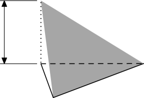
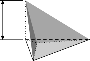
$\theta_{3}^{*}$$1$$\boldsymbol{x}_{1}$ $\boldsymbol{x}_{2}$$\boldsymbol{x}_{3}$    $\theta_{3}^{*}$$1$$\boldsymbol{x}_{1}$ $\boldsymbol{x}_{2}$$\boldsymbol{x}_{3}$$\boldsymbol{x}_{P}$

Figure 1. A graph of the approximate minimum energy extension $\theta^{*}_{n}$ for $\kappa_{K}\rho_{K}\leq 1$ (left) and for $\kappa_{K}\rho_{K}>1$ (right).

It is easy to verify that $\theta^{*}_{n}$, $n\in\{1,2,\dots,d+1\}$, satisfy

• $\theta^{*}_{n}=\theta_{n}$ on the boundary $\partial K$;

• if $\kappa_{K}\rho_{K}\leq 1$ then $\theta^{*}_{n}=\theta_{n}$ on $K$;

• $C_{1}h_{K}^{d-1}\min\{h_{K},1/\kappa_{K}\}\leq\left\|\theta^{*}_{n}\right\|_{K}^{2}\leq C_{2}h_{K}^{d-1}\min\{h_{K},1/\kappa_{K}\}$;

• $C_{1}h_{K}^{d-1}\min\{h_{K},1/\kappa_{K}\}^{-1}\leq\left\|\boldsymbol{\nabla}\theta^{*}_{n}\right\|_{K}^{2}\leq C_{2}h_{K}^{d-1}\min\{h_{K},1/\kappa_{K}\}^{-1}$.

These key features of the approximate minimum energy extensions $\theta^{*}_{n}$ were identified already in [6] and are crucial for the robustness of the resulting fluxes.

The robust flux reconstruction is obtained in [6] by replacing functions $\theta_{n}$ by $\theta^{*}_{n}$ in (22) and finding the least squares minimizer of the system. This approach must be modified to deal with case of variable $\kappa$ considered here.

First, we define

$$\varepsilon_{K}(\theta)=\mathcal{F}_{K}(\theta)-\mathcal{B}_{K}(u_{h},\theta)+\int_{\partial K\setminus{\Gamma_{\mathrm{N}}}}g_{K}\theta\,\mathrm{d}\boldsymbol{s}$$

for any $\theta\in H^{1}(K)$. The robust equlibration procedure requires

$$\varepsilon_{K}(\theta_{n})=0\quad\forall K\in\mathcal{T}_{h},\text{ where }\kappa_{K}\rho_{K}\leq 1,\text{ and }n=1,2,\dots,d+1.$$ (23)

For the other elements, we impose a similar condition in a least-squares sense. We obtain a constrained least-squares problem to find $g_{K}$ satisfying (19)–(21), equality constraints (23) and minimizing

$$\sum\limits_{K\in\mathcal{T}_{h}:\kappa_{K}\rho_{K}>1}\sum\limits_{n=1}^{d+1}\varepsilon_{K}(\theta^{*}_{n})^{2}.$$ (24)

This global constrained least-squares problem can be transformed into a series of small constrained least-squares problems on patches of elements corresponding to vertices of $\mathcal{T}_{h}$ as follows.

We define the set of vertices $\mathcal{N}(\gamma)$ of a facet $\gamma$ of a simplex $K$ and functions $\psi_{\gamma}^{m}\in\mathbb{P}^{1}(\gamma)$ satisfying $\int_{\gamma}\psi_{\gamma}^{m}\theta_{n}\,\mathrm{d}\boldsymbol{s}=\delta_{mn}.$ Further, we consider a fixed orientation $\sigma_{K,\gamma}$ of facets $\gamma$ of simplices $K\in\mathcal{T}_{h}$. The orientation $\sigma_{K,\gamma}$ is either $1$ or $-1$ and satisfies

$$\sigma_{K,\gamma}+\sigma_{K^{\prime},\gamma}=0\quad\text{on }\gamma=\partial K\cap\partial K^{\prime}.$$

Finally, we introduce the average and the jump flux across a common facet of two neighbouring simplices $K$ and $K^{\prime}$ as

$$\left\langle\frac{\partial u_{h}}{\partial\boldsymbol{n}_{K}}\right\rangle=\frac{1}{2}\boldsymbol{n}_{K}\cdot\left(\boldsymbol{\nabla}u_{h}|_{K}+\boldsymbol{\nabla}u_{h}|_{K^{\prime}}\right)\quad\text{and}\quad\left[\frac{\partial u_{h}}{\partial\boldsymbol{n}_{K}}\right]=\boldsymbol{n}_{K}\cdot\left(\boldsymbol{\nabla}u_{h}|_{K}-\boldsymbol{\nabla}u_{h}|_{K^{\prime}}\right).$$

On the boundary $\partial\Omega$ we set $\left\langle\partial u_{h}/\partial\boldsymbol{n}_{K}\right\rangle=\partial u_{h}/\partial\boldsymbol{n}_{K}$ and $[\partial u_{h}/\partial\boldsymbol{n}_{K}]=0$. The boundary flux $g_{K}$ on a facet $\gamma$ of a simplex $K$ is then defined in the form

$$g_{K}=\left\langle\frac{\partial u_{h}}{\partial\boldsymbol{n}_{K}}\right\rangle+\sigma_{K,\gamma}\sum\limits_{{}_{m}\in\mathcal{N}(\gamma)}\alpha_{\gamma}^{m}\psi_{\gamma}^{m}.$$ (25)

Notice that this construction of $g_{K}$ immediately guarantees the consistency condition (21). Furthermore, if $\gamma\subset{\Gamma_{\mathrm{N}}}$ then the coefficients $\alpha_{\gamma}^{m}$ are uniquely determined by (20).

Using (25), we can readily express $\varepsilon_{K}(\theta)$ as

$$\varepsilon_{K}(\theta)=D_{K}(\theta)+\sum\limits_{\gamma:\gamma\subset\partial K\setminus{\Gamma_{\mathrm{N}}},\gamma\ni\mbox{\boldmath$x$}_{n}}\sigma_{K,\gamma}\alpha^{n}_{\gamma},$$ (26)

where

$$D_{K}(\theta)=\mathcal{F}_{K}(\theta)-\mathcal{B}_{K}(u_{h},\theta)+\int_{\partial K\setminus{\Gamma_{\mathrm{N}}}}\left\langle\frac{\partial u_{h}}{\partial\boldsymbol{n}_{K}}\right\rangle\theta\,\mathrm{d}\boldsymbol{s}.$$

Note that the summation in (26) is performed over those facets $\gamma\subset\partial K\setminus{\Gamma_{\mathrm{N}}}$ that contain the vertex $\mbox{\boldmath$x$}_{n}$.

Thus, the global constrained least-squares problem (23)–(24) transforms into the following small local constrained least-squares problems on patches of elements. For all vertices $\mbox{\boldmath$x$}_{n}$ in the partition $\mathcal{T}_{h}$, we define $\omega(\mbox{\boldmath$x$}_{n})=\{K\in\mathcal{T}_{h}:\mbox{\boldmath$x$}_{n}\in\overline{K}\}$ to be the set of elements sharing the vertex $\mbox{\boldmath$x$}_{n}$ and seek coefficients $\alpha^{n}_{\gamma}$ for $\gamma\not\subset{\Gamma_{\mathrm{N}}}$, $\gamma\ni\mbox{\boldmath$x$}_{n}$ satisfying equality constraints

$$\varepsilon_{K}(\theta_{n})=0\quad\forall K\in\omega(\mbox{\boldmath$x$}_{n}),\text{where }\kappa_{K}\rho_{K}\leq 1,$$ (27)

and minimizing

$$\sum\limits_{K\in\omega(\mbox{\boldmath$x$}_{n}):\kappa_{K}\rho_{K}>1}\varepsilon_{K}(\theta^{*}_{n})^{2}.$$ (28)

Note that $\varepsilon_{K}$ in (27) and (28) is considered in the form (26).

Observe that the system (27)–(28) is always solvable. It was shown in [6] and [1] that if $\kappa_{K}\rho_{K}\leq 1$ for all elements $K\in\omega(\mbox{\boldmath$x$}_{n})$ then the linear system (27) is always solvable. Trivially, removing some (or all) equality constraints and replacing them by the requirement of least-squares fit (28), preserves the solvability of the remaining system of linear constraints (27). In case the constrained least-squared problem (27)–(28) does not have a unique solution, we consider the solution with the smallest $L^{2}$ norm.

To summarize, we require the satisfaction of the exact equilibration condition (27) for those elements where the coefficient $\kappa_{K}$ is small. For the other elements we mimic the equilibration by the least-squares fit (28). The resulting constrained least-squares problem (27)–(28) is always solvable and its solution depends continuously on the data.

3.4. Auxiliary results

In this section we recall several estimates from [6] and extend them to include the case of piecewise constant $\kappa$ and to Neumann boundary conditions. Let us note that assumptions (6)–(7) and consequently (8) make this extension straightforward. Lemma 5(2) from [6] says that if $\gamma$ is an interior facet (i.e. shared by two elements) then

$$\left\|\left[\frac{\partial u_{h}}{\partial\boldsymbol{n}_{K}}\right]\right\|_{\gamma}\leq C\left[\min\{h_{\gamma},\kappa_{K}^{-1}\}^{-\frac{1}{2}}|\!|\!|u-u_{h}|\!|\!|_{\widetilde{\gamma}}+\min\{h_{\gamma},\kappa_{K}^{-1}\}^{\frac{1}{2}}\left\|f-\Pi f\right\|_{\widetilde{\gamma}}\right],$$ (29)

where $\widetilde{\gamma}$ is the pair of elements sharing the facet $\gamma$ and $\Pi f$ is defined piecewise by $(\Pi f)|_{K}=\Pi_{K}f$ for all $K\in\mathcal{T}_{h}$. Notice that thanks to the assumption (8) estimate (29) holds for any $K\in\widetilde{\gamma}$.

Further, Lemma 6 from [6] provides the estimate

$$\left\|g_{K}-\left\langle\frac{\partial u_{h}}{\partial\boldsymbol{n}_{K}}\right\rangle\right\|_{\gamma}\leq C\left[\min\{h_{\gamma},\kappa_{K}^{-1}\}^{-\frac{1}{2}}|\!|\!|u-u_{h}|\!|\!|_{\widetilde{K}}+\min\{h_{\gamma},\kappa_{K}^{-1}\}^{\frac{1}{2}}\left\|f-\Pi f\right\|_{\widetilde{K}}\right],$$ (30)

for all $K\in\mathcal{T}_{h}$, where $\gamma$ is a facet of $K$ that is either interior or it lies on the Dirichlet boundary ${\Gamma_{\mathrm{D}}}$. The patch of elements $\widetilde{K}$ was defined in (4) and condition (8) is needed to generalize the proof from [6] to the case of piecewise constant $\kappa$. The final estimate on page 343 in [6] states that

$$\left\|\Pi_{K}r_{h}\right\|_{K}\leq C\left[\min\{h_{K},\kappa_{K}^{-1}\}|\!|\!|u-u_{h}|\!|\!|_{K}+\left\|f-\Pi_{K}f\right\|_{K}\right],$$ (31)

for all elements $K$ in $\mathcal{T}_{h}$. Here, $r_{h}=f-\kappa_{K}^{2}u_{h}+\Delta u_{h}$ stands for the residual on $K$. This bound is local and independent of values of $\kappa$ in the other elements and therefore applies to the case considered here.

We emphasize that estimates (29)–(31) are proved in [6] for the case of pure Dirichlet boundary conditions and constant coefficient $\kappa$. However, their proofs remain valid even in the presence of Neumann boundary conditions and due to the condition (8) also for piecewise constant $\kappa$. Nevertheless, estimate (30) is not valid for a facet on the Neumann boundary. We use a slight modification of the proof of Lemma 5(2) from [6] and derive the estimate

$$\left\|g_{K}-\boldsymbol{\nabla}u_{h}|_{K}\cdot\boldsymbol{n}_{K}\right\|_{\gamma}\leq C\left[\min\{h_{K},\kappa_{K}^{-1}\}^{-\frac{1}{2}}|\!|\!|u-u_{h}|\!|\!|_{K}\right.\\ \left.+\min\{h_{K},\kappa_{K}^{-1}\}^{\frac{1}{2}}\left\|f-\Pi_{K}f\right\|_{K}+\left\|g_{\mathrm{N}}-\Pi_{\gamma}g_{\mathrm{N}}\right\|_{\gamma}\right]$$ (32)

for those facets $\gamma$ of $K$ located on the Neumann boundary ${\Gamma_{\mathrm{N}}}$. Thus, defining $R=g_{K}-\boldsymbol{\nabla}u_{h}|_{K}\cdot\boldsymbol{n}_{K}$, using (29), (30), (32) and the fact that

$$R=g_{K}-\left\langle\frac{\partial u_{h}}{\partial\boldsymbol{n}_{K}}\right\rangle-\frac{1}{2}\left[\frac{\partial u_{h}}{\partial\boldsymbol{n}_{K}}\right]$$

we easily derive the estimate

$$\left\|R\right\|_{\partial K}\leq C\left(\min\{h_{K},\kappa_{K}^{-1}\}^{-\frac{1}{2}}|\!|\!|u-u_{h}|\!|\!|_{\widetilde{K}}\right.\\ \left.+\min\{h_{K},\kappa_{K}^{-1}\}^{\frac{1}{2}}\left\|f-\Pi f\right\|_{\widetilde{K}}+\left\|g_{\mathrm{N}}-\Pi^{K}_{\gamma}g_{\mathrm{N}}\right\|_{{\Gamma_{\mathrm{N}}}\cap\partial K}\right)$$ (33)

for all $K\in\mathcal{T}_{h}$. In view of notation (9) and thanks to the assumption (7) the above estimates hold even if $\kappa_{K}=0$.

3.5. Flux reconstruction #1

For each simplex $K\in\mathcal{T}_{h}$ on which $\kappa_{K}\rho_{K}\leq 1$, we use a reconstruction of the form

$$\boldsymbol{\tau}_{K}^{(1)}=\boldsymbol{\nabla}u_{h}|_{K}+\boldsymbol{\tau}_{K}^{\mathrm{L}}+\boldsymbol{\tau}_{K}^{\mathrm{Q}}.$$ (34)

The vector field $\boldsymbol{\tau}_{K}^{\mathrm{L}}$ is defined as

$$\boldsymbol{\tau}_{K}^{\mathrm{L}}=-\sum\limits_{n=1}^{d+1}\lambda_{n}\sum\limits_{\begin{subarray}{c}m=1\\ m\neq n\end{subarray}}^{d+1}R_{|\gamma_{m}}(\boldsymbol{x}_{n})\;|\boldsymbol{\nabla}\lambda_{m}|\;\boldsymbol{t}_{nm},$$ (35)

where $\boldsymbol{x}_{n}$, $n=1,2,\dots,d+1$, stand for vertices of $K$, $\gamma_{n}$ are the facets opposite to the vertices $\boldsymbol{x}_{n}$, $\lambda_{n}$ are the corresponding barycentric coordinates, $\boldsymbol{t}_{mn}=\boldsymbol{x}_{n}-\boldsymbol{x}_{m}$ denote the edge-vectors from $\boldsymbol{x}_{m}$ to $\boldsymbol{x}_{n}$, and function $R=g_{K}-\boldsymbol{\nabla}u_{h}|_{K}\cdot\boldsymbol{n}_{K}$ is affine on each facet of $K$. The quadratic vector field $\boldsymbol{\tau}_{K}^{\mathrm{Q}}$ is given by

$$\boldsymbol{\tau}_{K}^{\mathrm{Q}}=\frac{1}{d+1}\sum\limits_{n=1}^{d+1}\sum\limits_{\begin{subarray}{c}m=2\\ m>n\end{subarray}}^{d+1}\lambda_{m}\lambda_{n}\boldsymbol{t}_{mn}\boldsymbol{t}_{mn}^{T}\boldsymbol{\nabla}r(\overline{\boldsymbol{x}}_{K})$$ (36)

where $r=\Pi_{K}f-\kappa_{K}^{2}u_{h}$ is affine on $K$, and $\overline{\boldsymbol{x}}_{K}$ denotes the centroid of simplex $K$.

It can be easily shown that $\boldsymbol{\tau}_{K}^{\mathrm{L}}\cdot\boldsymbol{n}_{K}=R$ and $\boldsymbol{\tau}_{K}^{\mathrm{Q}}\cdot\boldsymbol{n}_{K}=0$ on each facet of $K$. Indeed, if we denote the outward normal unit vector to the facet $\gamma_{k}$ by $\boldsymbol{n}_{k}$ then the following identity holds

$$\boldsymbol{\tau}_{K}^{\mathrm{L}}\cdot\boldsymbol{n}_{k}|_{\gamma_{k}} =-\sum\limits_{\begin{subarray}{c}n=1\\ n\neq k\end{subarray}}^{d+1}\lambda_{n}R_{|\gamma_{k}}(\boldsymbol{x}_{n})\;|\boldsymbol{\nabla}\lambda_{k}|\;\boldsymbol{t}_{nk}\cdot\boldsymbol{n}_{k}$$

$$=\sum\limits_{\begin{subarray}{c}n=1\\ n\neq k\end{subarray}}^{d+1}\lambda_{n}R_{|\gamma_{k}}(\boldsymbol{x}_{n})\;\boldsymbol{t}_{nk}\cdot\boldsymbol{\nabla}\lambda_{k}=\sum\limits_{\begin{subarray}{c}n=1\\ n\neq k\end{subarray}}^{d+1}\lambda_{n}R_{|\gamma_{k}}(\boldsymbol{x}_{n})=R_{|\gamma_{k}},$$

where we use the facts that: $\lambda_{k}|_{\gamma_{k}}=0$; if $n\neq k$ then $\boldsymbol{t}_{nm}\cdot\boldsymbol{n}_{k}=0$ for $m\neq k$; $\boldsymbol{n}_{k}=-\boldsymbol{\nabla}\lambda_{k}/|\boldsymbol{\nabla}\lambda_{k}|$; and $\boldsymbol{t}_{nk}\cdot\boldsymbol{\nabla}\lambda_{k}=1$. Similarly, we show that

$$\boldsymbol{\tau}_{K}^{\mathrm{Q}}\cdot\boldsymbol{n}_{k}|_{\gamma_{k}}=\frac{1}{d+1}\sum\limits_{n=1}^{d+1}\sum\limits_{\begin{subarray}{c}m=2\\ m>n\end{subarray}}^{d+1}\lambda_{m}|_{\gamma_{k}}\lambda_{n}|_{\gamma_{k}}(\boldsymbol{t}_{mn}\cdot\boldsymbol{\nabla}r(\overline{\boldsymbol{x}}_{K}))(\boldsymbol{t}_{mn}\cdot\boldsymbol{n}_{k})=0,$$

because if $n=k$ then $\lambda_{n}|_{\gamma_{k}}=0$ and if $n\neq k$ then $m\neq k$ and $\boldsymbol{t}_{mn}\cdot\boldsymbol{n}_{k}=0$.

Lemma 3.

Let $K\in\mathcal{T}_{h}$ then the vector field $\boldsymbol{\tau}_{K}^{(1)}$ defined by (34), (35), and (36) satisfies $\boldsymbol{\tau}_{K}^{(1)}\cdot\boldsymbol{n}_{K}=g_{K}$ on all facets of $K$ and, if $\kappa_{K}\rho_{K}\leq 1$, then

$$\Pi_{K}f-\kappa_{K}^{2}u_{h}+\operatorname{div}\boldsymbol{\tau}_{K}^{(1)}=0\quad\text{in }K.$$

Proof.

The first assertion is a consequence of the foregoing arguments. Suppose $\kappa_{K}\rho_{K}\leq 1$, then since $\boldsymbol{\tau}_{K}^{\mathrm{L}}$ has constant divergence over the element $K$ and $\boldsymbol{\nabla}u_{h}|_{K}$ has vanishing divergence over $K$, we have

$$\operatorname{div}\boldsymbol{\tau}_{K}^{\mathrm{L}}=\frac{1}{|K|}\int_{\partial K}\boldsymbol{\tau}_{K}^{\mathrm{L}}\cdot\boldsymbol{n}_{K}\,\mathrm{d}\boldsymbol{s}=\frac{1}{|K|}\int_{\partial K}g_{K}\,\mathrm{d}\boldsymbol{s}.$$

Since $\kappa_{K}\rho_{K}\leq 1$, the exact equilibration condition (23) is satisfied in $K$ for $n=1,2,\dots,d+1$ and, consequently, using the fact that $\sum_{n=1}^{d+1}\theta_{n}=1$ on $K$ in (23) we end up with equality

$$\int_{\partial K}g_{K}\,\mathrm{d}\boldsymbol{s}=-\int_{K}(f-\kappa_{K}^{2}u_{h})\,\mathrm{d}\boldsymbol{x}=-\int_{K}(\Pi_{K}f-\kappa_{K}^{2}u_{h})\,\mathrm{d}\boldsymbol{x}.$$

Observing that $\operatorname{div}(\lambda_{m}\lambda_{n}\boldsymbol{t}_{mn})=\lambda_{m}-\lambda_{n}$ and that

$$\sum\limits_{n=1}^{d+1}\sum\limits_{\begin{subarray}{c}m=2\\ m>n\end{subarray}}^{d+1}\left(\lambda_{m}(\boldsymbol{x})-\lambda_{n}(\boldsymbol{x})\right)(\boldsymbol{x}_{n}-\boldsymbol{x}_{m})=-(d+1)(\boldsymbol{x}-\overline{\boldsymbol{x}}_{K}),$$

where $\boldsymbol{x}=\sum_{m=1}^{d+1}\boldsymbol{x}_{m}\lambda_{m}(\boldsymbol{x})$ and $\overline{\boldsymbol{x}}_{K}=\sum_{m=1}^{d+1}\boldsymbol{x}_{m}/(d+1)$, we can compute the divergence of $\boldsymbol{\tau}_{K}^{\mathrm{Q}}$ as

$$\operatorname{div}\boldsymbol{\tau}_{K}^{\mathrm{Q}}(\boldsymbol{x})=\frac{1}{d+1}\sum\limits_{n=1}^{d+1}\sum\limits_{\begin{subarray}{c}m=2\\ m>n\end{subarray}}^{d+1}(\lambda_{m}(\boldsymbol{x})-\lambda_{n}(\boldsymbol{x}))(\boldsymbol{x}_{n}-\boldsymbol{x}_{m})\cdot\boldsymbol{\nabla}r(\overline{\boldsymbol{x}}_{K})\\ =\left(\overline{\boldsymbol{x}}_{K}-\boldsymbol{x}\right)\cdot\boldsymbol{\nabla}r(\overline{\boldsymbol{x}}_{K}).$$

Using the fact that $r=\Pi_{K}f-\kappa_{K}^{2}u_{h}$ is affine and the centroid quadrature rule for simplices that is exact for all linear functions, we obtain

$$\operatorname{div}\boldsymbol{\tau}_{K}^{\mathrm{Q}}(\boldsymbol{x})=-r(\boldsymbol{x})+r(\overline{\boldsymbol{x}}_{K})=-r(\boldsymbol{x})+\frac{1}{|K|}\int_{K}r\,\mathrm{d}\boldsymbol{x}.$$

The statement of the lemma follows by summing the above equations. ∎

The next result shows that $\boldsymbol{\tau}_{K}^{(1)}$ gives an efficient estimate of the local error in element $K$:

Lemma 4.

If $K\in\mathcal{T}_{h}$ is such that $\kappa_{K}\rho_{K}\leq 1$ then

$$\eta_{K}\bigl{(}\boldsymbol{\tau}_{K}^{(1)}\bigr{)}\leq C\left(|\!|\!|u-u_{h}|\!|\!|_{\widetilde{K}}+h_{K}\left\|f-\Pi f\right\|_{\widetilde{K}}+h_{K}^{1/2}\left\|g_{\mathrm{N}}-\Pi^{K}_{\gamma}g_{\mathrm{N}}\right\|_{{\Gamma_{\mathrm{N}}}\cap\partial K}\right).$$

Proof.

Let

$$\boldsymbol{c}_{n}=\sum\limits_{\begin{subarray}{c}m=1\\ m\neq n\end{subarray}}^{d+1}R_{|\gamma_{m}}(\boldsymbol{x}_{n})\;|\boldsymbol{\nabla}\lambda_{m}|\;\boldsymbol{t}_{nm},$$

then $\boldsymbol{\tau}_{K}^{\mathrm{L}}=-\sum_{n=1}^{d+1}\lambda_{n}\boldsymbol{c}_{n}$ and we have

$$|\boldsymbol{c}_{n}|\leq\sum\limits_{\begin{subarray}{c}m=1\\ m\neq n\end{subarray}}^{d+1}|R_{|\gamma_{m}}(\boldsymbol{x}_{n})|\;|\boldsymbol{\nabla}\lambda_{m}|\;|\boldsymbol{t}_{nm}|\leq C\sum\limits_{\begin{subarray}{c}m=1\\ m\neq n\end{subarray}}^{d+1}|R_{|\gamma_{m}}(\boldsymbol{x}_{n})|,$$

because $d|K||\boldsymbol{\nabla}\lambda_{m}|=|\gamma_{m}|$, $|\boldsymbol{t}_{nm}|\leq h_{K}$, and due to the shape regularity assumption (3). Further, thanks to the linearity of $R$,

$$\sum\limits_{\begin{subarray}{c}n=1\\ n\neq m\end{subarray}}^{d+1}|R_{|\gamma_{m}}(\boldsymbol{x}_{n})|^{2}\leq C\frac{1}{|\gamma_{m}|}\left\|R\right\|_{\gamma_{m}}^{2}.$$

We utilize these results to bound

$$\left\|\boldsymbol{\tau}_{K}^{\mathrm{L}}\right\|_{K}^{2}\leq C|K|\sum\limits_{n=1}^{d+1}|\boldsymbol{c}_{n}|^{2}\leq C|K|\sum\limits_{m=1}^{d+1}\sum\limits_{\begin{subarray}{c}n=1\\ n\neq m\end{subarray}}^{d+1}|R_{|\gamma_{m}}(\boldsymbol{x}_{n})|^{2}\leq Ch_{K}\left\|R\right\|_{\partial K}^{2}.$$ (37)

Similarly, we have

$$\left\|\boldsymbol{\tau}_{K}^{\mathrm{Q}}\right\|_{K}^{2}\leq C\sum\limits_{n=1}^{d+1}\sum\limits_{\begin{subarray}{c}m=2\\ m>n\end{subarray}}^{d+1}\int\limits_{K}\lambda_{m}^{2}\lambda_{n}^{2}\,\mathrm{d}\boldsymbol{x}|\boldsymbol{t}_{mn}|^{4}|\boldsymbol{\nabla}r|^{2}\leq Ch_{K}^{4}|K|\;|\boldsymbol{\nabla}r|^{2}\leq Ch_{K}^{4}\left\|\boldsymbol{\nabla}r\right\|_{K}^{2},$$

where we used the fact that $\boldsymbol{\nabla}r$ is constant over $K$. Since $r\in\mathbb{P}^{1}(K)$, we have the inverse inequality $\left\|\boldsymbol{\nabla}r\right\|_{K}\leq Ch_{K}^{-1}\left\|r\right\|_{K}$ and we obtain

$$\left\|\boldsymbol{\tau}_{K}^{\mathrm{Q}}\right\|_{K}\leq Ch_{K}\left\|r\right\|_{K}=Ch_{K}\left\|\Pi_{K}r_{h}\right\|_{K},$$ (38)

because $r_{h}=f-\kappa_{K}^{2}u_{h}+\Delta u_{h}$ and $\Pi_{K}r_{h}=r$ on $K$.

Finally, using estimate (33) in (37) and estimate (31) in (38), we derive

$$\left\|\boldsymbol{\tau}_{K}^{\mathrm{L}}\right\|_{K} \leq C\left[|\!|\!|u-u_{h}|\!|\!|_{\widetilde{K}}+h_{K}\left\|f-\Pi f\right\|_{\widetilde{K}}+h_{K}^{1/2}\left\|g_{\mathrm{N}}-\Pi^{K}_{\gamma}g_{\mathrm{N}}\right\|_{{\Gamma_{\mathrm{N}}}\cap\partial K}\right],$$ (39)

$$\left\|\boldsymbol{\tau}_{K}^{\mathrm{Q}}\right\|_{K} \leq C\left[|\!|\!|u-u_{h}|\!|\!|_{K}+h_{K}\left\|f-\Pi f\right\|_{K}\right].$$ (40)

Notice that the assumption $\kappa_{K}\rho_{K}\leq 1$ and the shape regularity (3) imply the existence of a constant $C>0$ such that $Ch_{K}\leq\min\{h_{K},\kappa_{K}^{-1}\}\leq h_{K}$. Due to Lemma 3 and definition (17) we have

$$\eta_{K}(\boldsymbol{\tau}_{K}^{(1)})=\left\|\boldsymbol{\tau}_{K}^{(1)}-\boldsymbol{\nabla}u_{h}\right\|_{K}=\left\|\boldsymbol{\tau}_{K}^{\mathrm{L}}+\boldsymbol{\tau}_{K}^{\mathrm{Q}}\right\|_{K}\leq\left\|\boldsymbol{\tau}_{K}^{\mathrm{L}}\right\|_{K}+\left\|\boldsymbol{\tau}_{K}^{\mathrm{Q}}\right\|_{K}$$

and estimates (39)–(40) finish the proof. ∎

3.6. Flux reconstruction #2

On elements $K$ for which $\kappa_{K}\rho_{K}>1$, we use a flux reconstruction given by

$$\boldsymbol{\tau}_{K}^{(2)}=\boldsymbol{\nabla}u_{h}|_{K}+\boldsymbol{\tau}_{K}^{\mathrm{O}},$$ (41)

where the vector field $\boldsymbol{\tau}_{K}^{\mathrm{O}}$ is defined piecewise on each element $K$ in the following way. We consider $d+1$ subsimplices $K_{\gamma}$ of $K$ that are defined as convex hulls of the incentre $\boldsymbol{x}_{K}$ and facets $\gamma$ of $K$. In each subsimplex $K_{\gamma}$ we define $\boldsymbol{\tau}_{K}^{\mathrm{O}}$ to be

$$\boldsymbol{\tau}_{K}^{\mathrm{O}}(\boldsymbol{x})=\rho_{K}^{-1}(1-\kappa_{K}x_{d})^{+}(\boldsymbol{x}-\boldsymbol{x}_{K})R(x_{1},\dots,x_{d-1})\quad\text{in }K_{\gamma},$$

where $z^{+}=(|z|+z)/2$ stands for the positive part of $z$, $R=g_{K}-\boldsymbol{\nabla}u_{h}|_{K}\cdot\boldsymbol{n}_{K}$ as before, $\rho_{K}$ is the inradius of $K$, and $\boldsymbol{x}=(x_{1},x_{2},\dots,x_{d})$ are local Cartesian coordinates defined in such a way that points $(x_{1},\dots,x_{d-1})$ lie in the plane of $\gamma$ and $x_{d}$ corresponds to the direction perpendicular to $\gamma$ aiming inwards $K$, see Figure 2 for a three-dimensional illustration.

$x_{1}$$x_{2}$$x_{3}$$K_{\gamma}$$\gamma$$\boldsymbol{x}_{K}$$\rho_{K}$

Figure 2. Division of $K$ into subsimplices $K_{\gamma}$ and the local Cartesian coordinates.

Clearly, $\boldsymbol{\tau}_{K}^{\mathrm{O}}$ vanishes for $x_{d}\geq\kappa_{K}^{-1}$. We also observe that the normal component of $\boldsymbol{\tau}_{K}^{\mathrm{O}}$ vanishes on $\partial K_{\gamma}\setminus\gamma$ whilst on $\gamma$

$$\boldsymbol{\tau}_{K}^{\mathrm{O}}\cdot\boldsymbol{n}_{K}|_{\gamma}=R(x_{1},\dots,x_{d-1}),$$

because $x_{d}=0$ on $\gamma$ and $(\boldsymbol{x}-\boldsymbol{x}_{K})\cdot\boldsymbol{n}_{K}=\rho_{K}$ on $\gamma$. These conditions guarantee that $\boldsymbol{\tau}_{K}^{(2)}\in\boldsymbol{H}(\operatorname{div},K)$ and $\boldsymbol{\tau}_{K}^{(2)}\cdot\boldsymbol{n}_{K}=g_{K}$ on $\partial K$. Moreover, the flux leads to a locally efficient estimator for the error in the case $\kappa_{K}\rho_{K}>1$:

Lemma 5.

Let $K\in\mathcal{T}_{h}$ then $\boldsymbol{\tau}_{K}^{(2)}\cdot\boldsymbol{n}_{K}=g_{K}$ on $\partial K$ and, if $\kappa_{K}\rho_{K}>1$, then

$$\eta_{K}\bigl{(}\boldsymbol{\tau}_{K}^{(2)}\bigr{)}\leq C\left(|\!|\!|u-u_{h}|\!|\!|_{\widetilde{K}}+\kappa_{K}^{-1}\left\|f-\Pi f\right\|_{\widetilde{K}}+\kappa_{K}^{-1/2}\left\|g_{\mathrm{N}}-\Pi^{K}_{\gamma}g_{\mathrm{N}}\right\|_{{\Gamma_{\mathrm{N}}}\cap\partial K}\right).$$

Proof.

The first assertion has been shown above. Suppose $\kappa_{K}\rho_{K}>1$, then since $|\boldsymbol{x}-\boldsymbol{x}_{K}|\leq h_{K}$ and $h_{K}/\rho_{K}$ is bounded uniformly thanks to (3), we obtain

$$\left\|\boldsymbol{\tau}_{K}^{\mathrm{O}}\right\|_{K_{\gamma}}^{2}\leq\frac{h_{K}^{2}}{\rho_{K}^{2}}\int_{0}^{\kappa_{K}^{-1}}(1-\kappa_{K}x_{d})^{2}\,\mathrm{d}x_{d}\left\|R\right\|_{\gamma}^{2}=\frac{h_{K}^{2}}{\rho_{K}^{2}}\frac{1}{3\kappa_{K}}\left\|R\right\|_{\gamma}^{2}\leq C\kappa_{K}^{-1}\left\|R\right\|_{\gamma}^{2}.$$ (42)

For $x_{d}\leq\kappa_{K}^{-1}$, a simple computation yields inequality

$$|\operatorname{div}\boldsymbol{\tau}_{K}^{\mathrm{O}}|\leq\rho_{K}^{-1}(1-\kappa_{K}x_{d})^{+}\left(d|R|+h_{K}|\boldsymbol{\nabla}_{\gamma}R|\right)+\rho_{K}^{-1}\kappa_{K}h_{K}|R|,$$

where $\boldsymbol{\nabla}_{\gamma}$ denotes the gradient with respect to $x_{1},\dots,x_{d-1}$ only. Consequently,

$$\left\|\operatorname{div}\boldsymbol{\tau}_{K}^{\mathrm{O}}\right\|_{K_{\gamma}}^{2}\leq\frac{C}{\rho_{K}^{2}}\left(\int_{0}^{\kappa_{K}^{-1}}(1-\kappa_{K}x_{d})^{2}\,\mathrm{d}x_{d}\left[\left\|R\right\|_{\gamma}^{2}+h_{K}^{2}\left\|\boldsymbol{\nabla}_{\gamma}R\right\|_{\gamma}^{2}\right]+\kappa_{K}h_{K}^{2}\left\|R\right\|_{\gamma}^{2}\right).$$

Since $R\in\mathbb{P}^{1}(\gamma)$, we use the shape regularity and the inverse estimate $\left\|\boldsymbol{\nabla}_{\gamma}R\right\|_{\gamma}\leq Ch_{\gamma}^{-1}\left\|R\right\|_{\gamma}$ to derive

$$\left\|\operatorname{div}\boldsymbol{\tau}_{K}^{\mathrm{O}}\right\|_{K_{\gamma}}^{2}\leq\frac{C}{\rho_{K}^{2}}\frac{1}{\kappa_{K}}\max\{1,\kappa_{K}h_{K}\}^{2}\left\|R\right\|_{\gamma}^{2}\leq C\kappa_{K}\left\|R\right\|_{\gamma}^{2},$$ (43)

where the last inequality follows from the shape regularity (3), from (5), and from the assumption $\kappa_{K}\rho_{K}>1$.

Hence, thanks to (33) and (42):

$$\left\|\boldsymbol{\tau}_{K}^{(2)}-\boldsymbol{\nabla}u_{h}\right\|_{K}=\left\|\boldsymbol{\tau}_{K}^{\mathrm{O}}\right\|_{K}\leq C\kappa_{K}^{-1/2}\left\|R\right\|_{\partial K}\\ \leq C\left(|\!|\!|u-u_{h}|\!|\!|_{\widetilde{K}}+\kappa_{K}^{-1}\left\|f-\Pi f\right\|_{\widetilde{K}}+\kappa_{K}^{-1/2}\left\|g_{\mathrm{N}}-\Pi^{K}_{\gamma}g_{\mathrm{N}}\right\|_{{\Gamma_{\mathrm{N}}}\cap\partial K}\right).$$

Similarly, estimates (43), (31), and (33) yield the bound

$$\kappa_{K}^{-1}\left\|\Pi_{K}f-\kappa_{K}^{2}u_{h}+\operatorname{div}\boldsymbol{\tau}_{K}^{(2)}\right\|_{K}\leq\kappa_{K}^{-1}\left\|\Pi_{K}r_{h}\right\|_{K}+\kappa_{K}^{-1}\left\|\operatorname{div}\boldsymbol{\tau}_{K}^{\mathrm{O}}\right\|_{K}\\ \leq\kappa_{K}^{-1}\left\|\Pi_{K}r_{h}\right\|_{K}+C\kappa_{K}^{-1/2}\left\|R\right\|_{\partial K}\\ \leq C\left(|\!|\!|u-u_{h}|\!|\!|_{\widetilde{K}}+\kappa_{K}^{-1}\left\|f-\Pi f\right\|_{\widetilde{K}}+\kappa_{K}^{-1/2}\left\|g_{\mathrm{N}}-\Pi^{K}_{\gamma}g_{\mathrm{N}}\right\|_{{\Gamma_{\mathrm{N}}}\cap\partial K}\right).$$

Combining these estimates gives the result claimed. ∎

3.7. Main result

We combine the flux reconstructions $\boldsymbol{\tau}_{K}^{(1)}$ and $\boldsymbol{\tau}_{K}^{(2)}$ in a natural way and construct $\boldsymbol{\tau}\in\boldsymbol{H}(\operatorname{div},\Omega)$ elementwise as

$$\boldsymbol{\tau}|_{K}=\Bigl{\{}\begin{array}[]{ll}\boldsymbol{\tau}_{K}^{(1)}&\text{if }\kappa_{K}\rho_{K}\leq 1,\\ \boldsymbol{\tau}_{K}^{(2)}&\text{if }\kappa_{K}\rho_{K}>1,\end{array}$$ (44)

where $\boldsymbol{\tau}_{K}^{(1)}$ and $\boldsymbol{\tau}_{K}^{(2)}$ are defined in (34) and (41). The following theorem shows that the associated error estimator provides a guaranteed upper bound on the error, which is robust with respect to $\kappa$ and $h$.

Theorem 6.

Let $u$ be the exact weak solution given by (2) and and $u_{h}\in V_{h}$ be its finite element approximation (10). Let the flux reconstruction $\boldsymbol{\tau}\in\boldsymbol{H}(\operatorname{div},\Omega)$ be given by (44). Then the error in $u_{h}$ is bounded by

$$|\!|\!|u-u_{h}|\!|\!|^{2}\leq\eta^{2}(\boldsymbol{\tau})=\sum\limits_{K\in\mathcal{T}_{h}}\left[\eta_{K}(\boldsymbol{\tau})+\operatorname{osc}_{K}(f)+\operatorname{osc}_{{\Gamma_{\mathrm{N}}}\cap\partial K}(g_{\mathrm{N}})\right]^{2}.$$

Moreover, there exists a positive constant $C$, independent of any mesh-size or any values $\kappa_{K}$ satisfying (6)–(7), such that

$$\eta_{K}(\boldsymbol{\tau})\leq C\Bigl{(}|\!|\!|u-u_{h}|\!|\!|_{\widetilde{K}}+\min\{h_{K},\kappa_{K}^{-1}\}\left\|f-\Pi f\right\|_{\widetilde{K}}\\ +\min\{h_{K},\kappa_{K}^{-1}\}^{1/2}\left\|g_{\mathrm{N}}-\Pi^{K}_{\gamma}g_{\mathrm{N}}\right\|_{{\Gamma_{\mathrm{N}}}\cap\partial K}\Bigr{)}.$$

Proof.

It follows immediately from Lemmas 2, 4, and 5. ∎

In view of convention (9), this result holds even if $\kappa_{K}=0$ for any number of elements $K\in\mathcal{T}_{h}$. Theorem 6 provides a robust, computable upper bound, but it is possible to improve the bound at the expense of having to compute both $\eta_{K}(\boldsymbol{\tau}_{K}^{(1)})$ and $\eta_{K}(\boldsymbol{\tau}_{K}^{(2)})$ on every element. The associated flux is defined by

$$\boldsymbol{\tau}^{*}|_{K}=\Bigl{\{}\begin{array}[]{ll}\boldsymbol{\tau}_{K}^{(1)}&\text{if }\kappa_{K}=0\text{ or if }\eta_{K}(\boldsymbol{\tau}_{K}^{(1)})\leq\eta_{K}(\boldsymbol{\tau}_{K}^{(2)}),\\ \boldsymbol{\tau}_{K}^{(2)}&\text{otherwise}.\end{array}$$ (45)

and the corresponding estimator is given by $\eta(\boldsymbol{\tau}^{*})$, which in turn involves the local indicator $\eta_{K}(\boldsymbol{\tau}^{*})=\min\bigl{\{}\eta_{K}(\boldsymbol{\tau}_{K}^{(1)}),\eta_{K}(\boldsymbol{\tau}_{K}^{(2)})\bigr{\}}$. This flux reconstruction is slightly more expensive to compute, but it yields more accurate estimator than $\boldsymbol{\tau}$, because $\eta_{K}(\boldsymbol{\tau}^{*})\leq\eta_{K}(\boldsymbol{\tau})$. Clearly, if we replace $\boldsymbol{\tau}$ by $\boldsymbol{\tau}^{*}$ in Theorem 6, both its statements remain valid.

4. Numerical example

This section illustrates numerical performance of the a posteriori error estimators $\eta(\boldsymbol{\tau})$ and $\eta(\boldsymbol{\tau}^{*})$ for a three dimensional example. In particular, the example confirms the robustness of both estimators with respect to the discontinuous reaction coefficient $\kappa$ and with respect to the mesh size.

We consider problem (1) in a cube $\Omega=(-1,1)^{3}$, with piecewise constant coefficient $\kappa$ defined by

$$\kappa(x_{1},x_{2},x_{3})=\left\{\begin{array}[]{ll}\kappa_{1}&\text{ for }x_{1}<0,\\ \kappa_{2}&\text{ for }x_{1}\geq 0,\\ \end{array}\right.$$

where $0<\kappa_{1}\leq\kappa_{2}$ are constants. The right-hand side is $f=\kappa_{1}^{2}$. Homogeneous Dirichlet boundary conditions are assumed on ${\Gamma_{\mathrm{D}}}=\{(x_{1},x_{2},x_{3})\in\partial\Omega:x_{1}=\pm 1\}$ and homogeneous Neumann boundary conditions are prescribed on ${\Gamma_{\mathrm{N}}}=\partial\Omega\setminus{\Gamma_{\mathrm{D}}}$.

Its exact solution can be expressed as

$$u(x_{1},x_{2},x_{3})=\left\{\begin{array}[]{ll}A_{1}\mathrm{e}^{-\kappa_{1}x_{1}}+A_{2}\mathrm{e}^{\kappa_{1}x_{1}}+1&\text{ for }x_{1}<0,\\ A_{3}\mathrm{e}^{-\kappa_{2}x_{1}}+A_{4}\mathrm{e}^{\kappa_{2}x_{1}}+\kappa_{1}^{2}/\kappa_{2}^{2}&\text{ for }x_{1}\geq 0,\\ \end{array}\right.$$

where constants $A_{1},\dots,A_{4}$ are uniquely determined by the Dirichlet boundary conditions and by the requirement of $C^{1}$ continuity of $u(x_{1},x_{2},x_{3})$ for $x_{1}=0$. In the subsequent computations we fix $\kappa_{2}=10^{6}$ and hence the solution has a boundary layer at least in the vicinity of the face $x_{1}=1$. Although the true solution has a univariate nature, this plays no role in the computations.

We approximate this problem using linear finite elements on uniform tetrahedral meshes that are constructed in two steps. First, the cube $\Omega$ is uniformly divided into $M^{3}$ subcubes and then each subcube is split into 6 tetrahedrons along its diagonal. The resulting mesh then has $N_{\mathrm{DOF}}=(M-1)(M+1)^{2}$ degrees of freedom.

Figure 3 presents the results for a fixed mesh ($M=16$, $N_{\mathrm{DOF}}=4335$). The left panel shows the dependence of the true error $|\!|\!|u-u_{h}|\!|\!|$ and the error estimators $\eta(\boldsymbol{\tau})$ and $\eta(\boldsymbol{\tau}^{*})$ as $\kappa_{1}$ is varied in the range $(0,\kappa_{2}]$. The right panel presents the effectivity indices $I_{\mathrm{eff}}=\eta/|\!|\!|u-u_{h}|\!|\!|$. We observe that both estimators provide upper bound on the error and that they robustly capture the behaviour of the error in the whole range of values of $\kappa_{1}$. Thus, they are independent of the ratio $\kappa_{1}/\kappa_{2}$ in this case. As expected, the effectivity index for $\eta(\boldsymbol{\tau}^{*})$ is smaller than for $\eta(\boldsymbol{\tau})$. Both indices exhibit values around 2 for small values of $\kappa_{1}$ and they are close to 1 for $\kappa_{1}\geq 1000$.

 

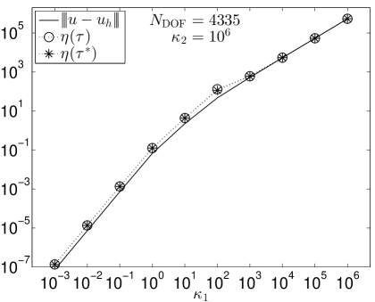
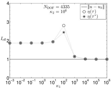
Figure 3. Dependence of $|\!|\!|u-u_{h}|\!|\!|$, $\eta(\boldsymbol{\tau})$, and $\eta(\boldsymbol{\tau}^{*})$ on $\kappa_{1}$ (left) and corresponding effectivity indices (right). These results correspond to $\kappa_{2}=10^{6}$ and to a mesh with $N_{\mathrm{DOF}}=4335$ ($M=16$).

Similarly, Figure 4 demonstrates the behaviour of these error estimators and of the true error with respect to the number of degrees of freedom. In this case we fix $\kappa_{1}=100$ and solve the problem on a series of meshes with $M=2,2^{2},2^{3},\dots,2^{7}$. We have chosen the most unfavourable value $\kappa_{1}=100$ for which both error estimators exhibit the highest overestimation in Figure 3.

As above, the left panel of Figure 4 presents the values of the true error $|\!|\!|u-u_{h}|\!|\!|$ and of the estimators $\eta(\boldsymbol{\tau})$ and $\eta(\boldsymbol{\tau}^{*})$, while the right panel shows the effectivity indices. Again, we verify the upper bound property of the estimators and observe their robust behaviour with respect to the mesh size. The effectivity indices have values around 1 and 2 with an exception of the intermediate case, where the mesh size $h$ is comparable to $1/\kappa_{1}$.

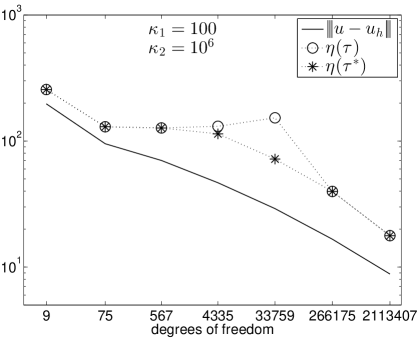
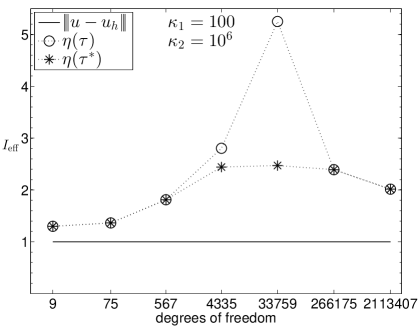
Figure 4. Dependence of $|\!|\!|u-u_{h}|\!|\!|$, $\eta(\boldsymbol{\tau})$, and $\eta(\boldsymbol{\tau}^{*})$ on the number of degrees of freedom (left) and corresponding effectivity indices (right). These results were computed on a sequence of uniformly refined meshes with $\kappa_{1}=100$ and $\kappa_{2}=10^{6}$.

5. Conclusions

We presented a robust a posteriori error estimator on the energy norm of the approximation error for a reaction-diffusion problem in arbitrary dimension. The reaction coefficient $\kappa$ is assumed to be piecewise constant and mixed Dirichlet-Neumann boundary conditions are allowed. The estimator is robust with respect to the reaction coefficient $\kappa$, including the singularly perturbed case, and it provides a computable upper bound on the error. The upper bound is guaranteed up to round-off errors and quadrature errors in the evaluation of $\eta(\boldsymbol{\tau})$.

The evaluation of the error estimator can be implemented as a fast algorithm in the sense that the computational complexity is proportional to the number of elements. Indeed, the boundary flux equilibration procedure described in Section 3.3 is fast, because it is based on solving small systems on patches. Flux reconstructions (34) and (41) are given by explicit formulas, hence, the only issue is to loop over all elements and compute the norms in (17).

The presented approach is suitable for the piecewise linear finite element approximations. The Galerkin condition (10) is required in order to guarantee the exact equilibration condition (23) in case of small values of the reaction coefficient $\kappa$. On the other hand, the exact equilibration is not needed for large values of $\kappa$ and the presented error estimator can be used for an arbitrary (conforming) approximate solution $u_{h}\in V$.

Finally, we note that whilst we have assumed conformity of the approximation, this is not essential. Methodologies derived in [25, 26, 27] could be used to extend the error bound to any piecewise linear non-conforming approximation.

References

References

- [1] M. Ainsworth, J. T. Oden, A posteriori error estimation in finite element analysis, Wiley, New York, 2000.
- [2] M. Ainsworth, T. Vejchodský, Fully computable robust a posteriori error bounds for singularly perturbed reaction–diffusion problems, Numer. Math. 119 (2) (2011) 219–243.
- [3] W. Dörfler, A convergent adaptive algorithm for Poisson’s equation, SIAM J. Numer. Anal. 33 (3) (1996) 1106–1124.
- [4] R. Verfürth, Robust a posteriori error estimators for a singularly perturbed reaction-diffusion equation, Numer. Math. 78 (3) (1998) 479–493.
- [5] R. Verfürth, A posteriori error estimators for convection-diffusion equations, Numer. Math. 80 (4) (1998) 641–663.
- [6] M. Ainsworth, I. Babuška, Reliable and robust a posteriori error estimating for singularly perturbed reaction-diffusion problems, SIAM J. Numer. Anal. 36 (2) (1999) 331–353 (electronic).
- [7] S. Grosman, An equilibrated residual method with a computable error approximation for a singularly perturbed reaction-diffusion problem on anisotropic finite element meshes, M2AN Math. Model. Numer. Anal. 40 (2) (2006) 239–267.
- [8] I. Cheddadi, R. Fučík, M. I. Prieto, M. Vohralík, Guaranteed and robust a posteriori error estimates for singularly perturbed reaction–diffusion problems, M2AN Math. Model. Numer. Anal. 43 (2009) 867–888.
- [9] T. Linss, A posteriori error estimation for arbitrary-order FEM applied to singularly perturbed one-dimensional reaction-diffusion problems, Appl. Math. To appear, 2014.
- [10] J. L. Synge, The hypercircle in mathematical physics: a method for the approximate solution of boundary value problems, Cambridge University Press, New York, 1957.
- [11] J. P. Aubin, H. G. Burchard, Some aspects of the method of the hypercircle applied to elliptic variational problems, in: Numerical Solution of Partial Differential Equations, II (SYNSPADE 1970) (Proc. Sympos., Univ. of Maryland, College Park, Md., 1970), Academic Press, New York, 1971, pp. 1–67.
- [12] J. Haslinger, I. Hlaváček, Convergence of a finite element method based on the dual variational formulation, Apl. Mat. 21 (1) (1976) 43–65.
- [13] B. F. de Veubeke, Displacement and equilibrium models in the finite element method, in: O. Zienkiewicz, G. Hollister (Eds.), Stress Analysis, Wiley, London, 1965, pp. 145–197.
- [14] S. Repin, A posteriori estimates for partial differential equations, Vol. 4 of Radon Series on Computational and Applied Mathematics, Walter de Gruyter GmbH & Co. KG, Berlin, 2008.
- [15] D. Braess, J. Schöberl, Equilibrated residual error estimator for edge elements, Math. Comp. 77 (262) (2008) 651–672.
- [16] Z. Cai, S. Zhang, Flux recovery and a posteriori error estimators: conforming elements for scalar elliptic equations, SIAM J. Numer. Anal. 48 (2) (2010) 578–602.
- [17] P. Jiránek, Z. Strakoš, M. Vohralík, A posteriori error estimates including algebraic error and stopping criteria for iterative solvers, SIAM J. Sci. Comput. 32 (3) (2010) 1567–1590.
- [18] D. W. Kelly, The self-equilibration of residuals and complementary a posteriori error estimates in the finite element method, Internat. J. Numer. Methods Engrg. 20 (8) (1984) 1491–1506.
- [19] P. Ladevèze, D. Leguillon, Error estimate procedure in the finite element method and applications, SIAM J. Numer. Anal. 20 (3) (1983) 485–509.
- [20] N. Parés, H. Santos, P. Díez, Guaranteed energy error bounds for the Poisson equation using a flux-free approach: Solving the local problems in subdomains, Internat. J. Numer. Methods Engrg. 79 (10) (2009) 1203–1244.
- [21] M. Vohralík, Guaranteed and fully robust a posteriori error estimates for conforming discretizations of diffusion problems with discontinuous coefficients, J. Sci. Comput. 46 (3) (2011) 397–438.
- [22] L. E. Payne, H. F. Weinberger, An optimal Poincaré inequality for convex domains, Arch. Rational Mech. Anal. 5 (1960) 286–292 (1960).
- [23] I. Šebestová, T. Vejchodský, Two-sided bounds for eigenvalues of differential operators with applications to Friedrichs, Poincaré, trace, and similar constants, SIAM J. Numer. Anal. 52 (1) (2014) 308–329.
- [24] V. Dolejší, M. Feistauer, C. Schwab, A finite volume discontinuous Galerkin scheme for nonlinear convection-diffusion problems, Calcolo 39 (1) (2002) 1–40.
- [25] M. Ainsworth, Robust a posteriori error estimation for nonconforming finite element approximation, SIAM J. Numer. Anal. 42 (6) (2005) 2320–2341 (electronic).
- [26] M. Ainsworth, A posteriori error estimation for discontinuous Galerkin finite element approximation, SIAM J. Numer. Anal. 45 (4) (2007) 1777–1798 (electronic).
- [27] A. Ern, A. F. Stephansen, M. Vohralík, Guaranteed and robust discontinuous Galerkin a posteriori error estimates for convection-diffusion-reaction problems, J. Comput. Appl. Math. 234 (1) (2010) 114–130.