Molecular Outflows Driven by Low-Mass Protostars. I. Correcting for Underestimates When Measuring Outflow Masses and Dynamical Properties

Abstract

We present a survey of 28 molecular outflows driven by low-mass protostars, all of which are sufficiently isolated spatially and/or kinematically to fully separate into individual outflows. Using a combination of new and archival data from several single-dish telescopes, 17 outflows are mapped in ¹²CO (2–1) and 17 are mapped in ¹²CO (3–2), with 6 mapped in both transitions. For each outflow, we calculate and tabulate the mass ($M_{\rm flow}$), momentum ($P_{\rm flow}$), kinetic energy ($E_{\rm flow}$), mechanical luminosity ($L_{\rm flow}$), and force ($F_{\rm flow}$) assuming optically thin emission in LTE at an excitation temperature, $T_{\rm ex}$, of 50 K. We show that all of the calculated properties are underestimated when calculated under these assumptions. Taken together, the effects of opacity, outflow emission at low velocities confused with ambient cloud emission, and emission below the sensitivities of the observations increase outflow masses and dynamical properties by an order of magnitude, on average, and factors of 50–90 in the most extreme cases. Different (and non-uniform) excitation temperatures, inclination effects, and dissociation of molecular gas will all work to further increase outflow properties. Molecular outflows are thus almost certainly more massive and energetic than commonly reported. Additionally, outflow properties are lower, on average, by almost an order of magnitude when calculated from the ¹²CO (3–2) maps compared to the ¹²CO (2–1) maps, even after accounting for different opacities, map sensitivities, and possible excitation temperature variations. It has recently been argued in the literature that the ¹²CO (3–2) line is subthermally excited in outflows, and our results support this finding.

1. Introduction

Bipolar molecular outflows from protostars, first detected more than 30 years ago (Snell et al., 1980), are ubiquitous in the star formation process (e.g., Hatchell et al., 2007a; Hatchell & Dunham, 2009). They are associated with both low and high-mass star formation (Wu et al., 2004), and have even recently been detected in the substellar regime (Phan-Bao et al., 2008, 2011). Since they are driven by accretion (e.g., Cabrit & Bertout, 1992; Bontemps et al., 1996), molecular outflows can be used to measure the time-averaged accretion histories of their driving sources (Dunham et al., 2006, 2010; Lee et al., 2010). They also carry away excess angular momentum, remove circumstellar material and shape the stellar initial mass function (IMF), and inject momentum and energy into the surrounding medium (e.g., Lada, 1985; Bachiller, 1996; Arce et al., 2007; Banerjee et al., 2007; Nakamura & Li, 2007; Hatchell et al., 2007a; Cunningham et al., 2009; Nakamura et al., 2011; Plunkett et al., 2013), although the efficiency with which they accomplish each of these remains under debate.

Developing a complete understanding of the roles molecular outflows play in each of the above processes requires accurate measurements of the morphologies, masses, and energetics of outflows located in a diverse range of environments and driven by sources over all stages of protostellar evolution. Numerous outflow surveys have been presented over the last three decades that have greatly improved our knowledge and understanding of the importance of outflows in the star formation process. These studies have revealed correlations between outflow strengths and the properties of their driving sources (Cabrit & Bertout, 1992; Bontemps et al., 1996; Wu et al., 2004; Hatchell et al., 2007a; Curtis et al., 2010b) and have directly measured the turbulent energy injected by outflows into their parent clusters (e.g., Arce et al., 2010; Nakamura et al., 2011; Ginsburg et al., 2011; Plunkett et al., 2013). However, since mapping the large extents of molecular outflows (which often have projected angular extents on the sky in excess of several arcminutes) to the sensitivies required to detect weak, high-velocity emission is necessarily expensive in terms of observing time, most of these studies suffer from one or more of the following limitations: (1) Observations that only cover the central regions and do not map the full extent of the outflows; (2) Difficulty separating overlapping outflows along the line of sight in clustered regions; and (3) Compiling outflow masses and dynamical properties from previously published studies that adopt different methods and make different assumptions, leading to a heterogeneous dataset.

The simplest method to calculate the masses and dynamical properties of molecular outflows is to assume that the emission from outflowing gas in low-J rotational transitions of ¹²CO is optically thin, in local thermodynamic equilibrium at a single excitation temperature, and confined to velocities larger than those dominated by ambient cloud emission. However, both Downes & Cabrit (2007) and Offner et al. (2011) used synthetic observations of simulated outflows to show that the effects of line opacity, excitation temperature variations, low-velocity outflow emission confused with ambient cloud emission, inclination, and dissociation of molecular gas can increase outflow masses and dynamical properties by one or more orders of magnitude compared to the values obtained under the simple assumptions listed above. The extent to which outflow surveys account for, and the methods they use to correct for, these effects vary widely from one to the next. Specific examples will be discussed in the following sections of this paper, but most suffer from one or more of the limitations discussed above. Indeed, a complete quantification of the magnitude of the corrections for all these effects with a large, statistically significant sample of well-separated outflows mapped in their entirety and analyzed with uniform methodology is currently lacking from the literature. In light of the results of Downes & Cabrit (2007) and Offner et al. (2011), such a study is clearly needed.

With these motivations, we have undertaken a survey of 28 molecular outflows driven by low-mass protostars, all of which are sufficiently isolated spatially and/or kinematically to fully separate into individual outflows. Using a combination of new and archival data from several single-dish telescopes, 17 outflows are mapped in ¹²CO (2–1) and 17 are mapped in ¹²CO (3–2), with 6 mapped in both transitions. Additional ¹³CO observations are obtained for selected outflows. In this paper we present an overview of the data collection and analysis. We then calculate the masses and dynamical properties of all the outflows in a standard way assuming isothermal, optically thin emission in LTE. We follow this with a detailed investigation of the correction factors to these quantities that are necessary for the various effects listed above, derived directly from our data. In a forthcoming paper we will explore the effects of these corrections on our current understanding of the evolution of protostellar outflows and the link between the accretion and outflow processes (M. M. Dunham et al. 2014, in preparation).

The organization of this paper is as follows. We present an overview of the data collection and analysis in §2, including the philosophy behind our target selection in §2.1, the observation strategy for the ¹²CO maps (§2.2) and the selected ¹³CO observations (§2.3), and the data reduction methods (§2.4). Our basic results are given in §3, with §3.1 focusing on outflow geometrical properties and §3.2 giving details on our calculataion of the masses and dynamical properties under the simple assumptions listed above. We discuss the necessary corrections that must be applied to the outflow masses and dynamical properties in §4 for the effects of opacity (§4.1), different (and non-uniform) excitation temperatures (§4.2), low-velocity outflow emission confused with ambient cloud emission (§4.3), and emission below the sensitivities of the observations (§4.4). In §4.5 we discuss other possible corrections that we are not able to derive from our data, including those due to inclination, dissociation of molecular gas, and calculation methods. We provide a final overview and synthesis of the net effect of these corrections in §5.1, and compare results from the two transitions of ¹²CO in §5.2. Finally, we summarize our results and outline necessary future work in §6.

2. Description of the Data

2.1. Target Selection

Table 1List of Targets

	Map Center	Map Center
	R.A.	Decl.	Distance (Reference)	Rest Velocity
Source	J2000	J2000	(pc)	(km s-1)
IRAS 03235$+$3004	03 26 37.6	$+$30 15 24.2	250 (1)	$+$5.1
IRAS 03271$+$3013	03 30 15.5	$+$30 23 43.0	250 (1)	$+$5.9
IRAS 03282$+$3035	03 31 21.0	$+$30 45 27.8	250 (1)	$+$7.1
HH211	03 43 56.8	$+$32 00 50.3	250 (1)	$+$9.1
IRAS 04166$+$2706	04 19 43.6	$+$27 13 38.0	140 (2)	$+$6.7
IRAM 04191$+$1522	04 21 56.9	$+$15 29 45.9	140 (2)	$+$6.7
HH25/26	05 46 04.9	$-$00 14 52.0	430 (3)	$+$10.1
BHR86	13 07 37.2	$-$77 00 09.0	178 (4)	$+$3.7
IRAS 15398$-$3359	15 43 01.3	$-$34 09 15.0	150 (5)	$+$5.1
Lupus 3 MMS	16 09 18.1	$-$39 04 53.4	200 (5)	$+$4.8
L1709-SMM1/5	16 31 35.6	$-$24 01 29.3	125 (6)	$+$2.5
CB68	16 57 20.0	$-$16 09 22.2	130 (7)	$+$5.2
L483	18 17 30.0	$-$04 39 40.0	200 (8)	$+$5.4
Aqu-MM2/3/5	18 29 15.0	$-$01 40 30.0	260 (9)	$+$9.0
SerpS-MM13	18 30 01.5	$-$02 10 23.3	260 (9)	$+$8.0
CrA-IRAS32	19 02 58.7	$-$37 07 35.9	130 (10)	$+$5.6
L673-7	19 21 34.8	$+$11 21 23.0	240 (11)	$+$7.1
B335	19 37 00.9	$+$07 34 09.8	150 (12)	$+$8.3
L1152	20 35 46.6	$+$67 53 03.9	325 (13)	$+$2.5
L1157	20 39 06.2	$+$68 02 15.0	300 (13)	$+$2.6
L1228	20 57 19.9	$+$77 36 00.0	200 (14)	$-$8.0
L1014	21 24 07.6	$+$49 59 08.9	258 (11)	$+$4.2
L1165	22 06 50.7	$+$59 02 47.0	300 (15)	$-$1.6
L1251A-IRS3	22 30 31.9	$+$75 14 08.8	300 (16)	$-$3.9

The observations presented in this paper are a combination of new observations obtained from several single-dish (sub)millimeter telescopes and existing observations taken from telescope archives or provided by the authors of previously published data. Given the motivations for this study described above in §1, we select targets based on the following three criteria: (1) a molecular outflow is either already known to exist or strongly suspected based on previous observations, (2) the outflow is sufficiently isolated spatially and/or kinematically from nearby outflows to prevent any issues with confusion when deriving properties, and (3) the full sample must span large ranges in both the bolometric luminosity and evolutionary status of the driving sources.

In total, we present maps of 28 outflows, 17 of which were mapped in ¹²CO (2–1) and 17 in ¹²CO (3–2) (6 were mapped in both transitions). These outflows are listed in Table 1, which lists the name of the driving source, the Right Ascension and Declination of the center of the map, the distance to the source (and reference for this distance), and rest velocity of the source. All positions in the rest of the paper that are given in arcseconds of offset are relative to the positions listed in Table 1. A brief summary of the literature on each source is given in Appendix A. Further properties of the driving sources, including updated measurements of their bolometric luminosities and evolutionary status, will be given in a forthcoming paper aimed at compiling accurate, up-to-date measurements of source properties and evaluating the evolution of outflow activity from protostars.

2.2. ¹²CO Observations

Table 2Observation Log

			Observation	Map Size	$\delta$v	1$\sigma$ rms	JCMT	JCMT
Source	Telescope	Transition	Date	(arcmin2)	(km s-1)	(K)	Program	Map Type
L1709-SMM1/5	APEX	12CO (2–1)	2012 Apr	25	0.1	0.75	$\cdots$	$\cdots$
CB68	APEX	12CO (2–1)	2012 Apr	25	0.1	0.72	$\cdots$	$\cdots$
Aqu-MM2/3/5	APEX	12CO (2–1)	2012 Apr	81	0.1	0.50	$\cdots$	$\cdots$
SerpS-MM13	APEX	12CO (2–1)	2012 Apr	40	0.1	0.55	$\cdots$	$\cdots$
CrA-IRAS32	APEX	12CO (2–1)	2012 Apr	25	0.1	0.79	$\cdots$	$\cdots$
L673-7	APEX	12CO (2–1)	2011 Oct, Nov	37	0.1	0.20	$\cdots$	$\cdots$
L673-7	APEX	12CO (3–2)	2012 Apr,	37	0.1	0.50	$\cdots$	$\cdots$
			May, Jun				$\cdots$	$\cdots$
L673-7	APEX	13CO (3–2)	2012 Jun,	37	0.1	0.40	$\cdots$	$\cdots$
			Jul, Oct				$\cdots$	$\cdots$
BHR86	ASTE	12CO (3–2)	2011 Jun	60	0.5	0.08	$\cdots$	$\cdots$
Lupus 3 MMS	ASTE	12CO (3–2)	2011 Jun	25	0.5	0.11	$\cdots$	$\cdots$
L483	ASTE	12CO (3–2)	2011 Jun	10	0.5	0.05	$\cdots$	$\cdots$
IRAS 03235$+$3004	CSO	12CO (2–1)	2012 Oct	25	0.1	0.32	$\cdots$	$\cdots$
IRAS 03282$+$3035	CSO	12CO (2–1)	2012 Oct	27	0.1	0.28	$\cdots$	$\cdots$
HH211	CSO	12CO (2–1)	2012 Oct	12	0.1	0.25	$\cdots$	$\cdots$
L1152	CSO	12CO (2–1)	2012 Oct	25	0.1	0.23	$\cdots$	$\cdots$
L1157	CSO	12CO (2–1)	2012 Oct	26	0.1	0.32	$\cdots$	$\cdots$
L1165	CSO	12CO (2–1)	2012 Oct	31	0.1	0.34	$\cdots$	$\cdots$
L1157	CSO	12CO (3–2)	2012 Oct	16	0.1	1.6	$\cdots$	$\cdots$
IRAS 03235$+$3004	JCMT	12CO (3–2)	2007 Oct	3.5	0.1	0.29	M07BU08	Jiggle
IRAS 03271$+$3013	JCMT	12CO (3–2)	2007 Oct	3.5	0.1	0.35	M07BU08	Jiggle
IRAS 03282$+$3035	JCMT	12CO (3–2)	2007 Oct	3.5	0.1	0.53	M07BU08	Jiggle
HH211	JCMT	12CO (3–2)	2007 Dec	25	0.1	1.8	M06BGT02	Raster
IRAS 04166$+$2706	JCMT	12CO (3–2)	2007 Nov, 2009 Jan	180	0.5	0.48	GBS, M08BU26	Raster
IRAM 04191$+$1522	JCMT	12CO (3–2)	2008 Feb	24	0.5	0.23	M08AC08	Raster
HH25/26	JCMT	12CO (3–2)	2009 Jan	21	0.5	0.20	M08BU26	Raster
IRAS 15398$-$3359	JCMT	12CO (3–2)	2008 Jun	3.5	0.1	0.47	M08AN05	Jiggle
L1228	JCMT	12CO (3–2)	2008 Aug, Oct, Nov	105	1.0	0.33	M08BU11	Raster
L1014	JCMT	12CO (3–2)	2008 Jun	4	0.5	0.05	M08AC08	Jiggle
L1165	JCMT	12CO (3–2)	2008 Jun	49	0.5	0.24	M08AC03	Raster
L1251A-IRS3	SRAO	12CO (2–1)	2009 Mar, Apr	160	0.2	0.17	$\cdots$	$\cdots$
B335	SMT	12CO (2–1)	2007 Apr	192	0.33	0.14	$\cdots$	$\cdots$

In this section we summarize the observational details for the new and archival ¹²CO data used in this study. All brightness temperatures given in this paper are in units of $T_{\rm mb}$. Assumed or measured values of $\eta_{\rm mb}$ for each telescope are listed and generally include a 10% – 20% calibration uncertainty. Table 2 lists, for each map, the telescope used to obtain the map, the ¹²CO transition mapped, the observation date, the map size, the spectral resolution, and the 1$\sigma$ rms at this spectral resolution. Also listed are additional details for the JCMT observations (see §2.2.4 below). Entries in Table 2 are organized by telescope rather than by source. Finally, one ¹³CO map is also listed and is described in more detail in §2.3.

2.2.1 Atacama Pathfinder Experiment

A ¹²CO (2–1) map of L673-7 was obtained at the Atacama Pathfinder Experiment (APEX) in 2011 October and November through APEX program C-088.F-1752B-2011. Additional ¹²CO (2–1) maps of Oph IRS 63, CB68, Aqu-MM2/3/5, SerpS-MM13, and CrA-IRAS32 were obtained at APEX in 2012 April through APEX program C-089.F-9757B-2012. All data were obtained with the 230 GHz APEX-1 band of the Swedish Heterodyne Facility Instrument (SHeFi; Belitsky et al., 2006; Risacher et al., 2006) and the XFFTS fast fourier transform spectrometer, providing 2.5 GHz (3252 km s^-1) total bandwidth and 76 kHz (0.1 km s^-1) spectral resolution. The beam FWHM is 27″ at 230 GHz, and the main-beam efficiency, $\eta_{\rm mb}$, is 0.82 (Vassilev et al., 2008). All sources were mapped using the position-switched on-the-fly (otf) observing mode, with every second map observed at a position angle of 90^∘ relative to the first.

A ¹²CO (3–2) otf map of L673-7 was also obtained at APEX in 2012 April, May, and June through APEX program C-089.F-9758B-2012 with the 345 GHz APEX-2 band of SHeFI and the XFFTS backend, providing 2.5 GHz (2167 km s^-1) total bandwidth and 76 kHz (0.07 km s^-1) spectral resolution. The beam FWHM is 18″ at 345 GHz and $\eta_{\rm mb}$ is 0.73 (Güsten et al., 2006). The final map was smoothed to Nyquist sampled ($\sim 9$″) pixels.

2.2.2 Atacama Submillimeter Telescope Experiment

Maps of ¹²CO (3–2) of BHR86, Lupus 3 MMS, and L483 were obtained at the Atacama Submillimeter Telescope Experiment (ASTE) (Ezawa et al., 2004) in 2011 June through the program CN2011B-070 with the CATS345 receiver and MAC digital spectro-correlator configured to provide 512 MHz (445 km s^-1) bandwidth and 0.5 MHz (0.43 km s^-1) spectral resolution. The beam FWHM is 21.5″ at 345 GHz and $\eta_{\rm mb}$ $=0.6\pm 0.1$ (e.g., Nakamura et al., 2011; Miura et al., 2012; Watanabe et al., 2012). The maps were obtained using the position-switched otf observing mode, again with successive scans observed at perpendicular position angles. The final maps were smoothed to 11″ (approximately Nyquist sampled) pixels.

2.2.3 Caltech Submillimeter Observatory

Maps of ¹²CO (2–1) of IRAS 03235$+$3004, IRAS 03282$+$3035, HH211, L1152, L1157, and L1165 were obtained at the Caltech Submillimeter Observatory (CSO) in 2012 October with the 230 GHz sidecab receiver and a fast fourier transform spectrometer (FFTS) backend, providing 500 MHz (650 km s^-1) total bandwidth and 61 kHz (0.08 km s^-1) sectral resolution. The beam FWHM is 32.5″ at 230 GHz, and $\eta_{\rm mb}$ $=0.73\pm 0.02$ based on observations of Jupiter. Position-switched otf maps were obtained for each source, with successive scans observed at perpendicular position angles. The final maps were smoothed to Nyquist sampled ($\sim 16$″) pixels.

A ¹²CO (3–2) map of L1157 was also obtained at the CSO in 2012 October with the 345 GHz Barney receiver and FFTS backend, again providing a native spectral resolution of 61 kHz (0.05 km s^-1at 345 GHz). The beam FWHM is 22″, and $\eta_{\rm mb}$ $=0.74\pm 0.03$ based on observations of Jupiter. The final map was smoothed to Nyquist sampled ($\sim 11$″) pixels.

2.2.4 James Clerk Maxwell Telescope

Maps of ¹²CO (3–2) of IRAM 04191$+$1522 and L1014 were obtained at the James Clerk Maxwell Telescope (JCMT) in 2008 February and June with the Heterodyne Array Receiver Program B (HARP-B) band receiver (Buckle et al., 2009) and Auto-Correlation Spectral Imaging System (ACSIS; Dent et al., 2000; Buckle et al., 2009) backend through the JCMT observing program M08AC08. Additionally, ¹²CO (3–2) maps of nine sources (IRAS 03235$+$3004, IRAS 03271$+$3013, IRAS 03282$+$3035, HH211, IRAS 04166$+$2706, HH25/26, IRAS 15398$-$3359, L1228, and L1165) that were obtained in other programs with HARP-B and the ACSIS backend were taken from the JCMT data archive. HARP-B is a 16 element heterodyne receiver array arranged in a $4\times 4$ grid with 30″ spacing between elements. The beam FWHM is 14″ at 345 GHz (Buckle et al., 2009), and $\eta_{\rm mb}$ is taken to be 0.60 $\pm$ 0.02 (mean and standard deviation of each individual receiver in the array; Buckle et al., 2009). The data were taken in either the position-switched jiggle or raster map observing modes in a variety of backend configurations, and the final maps were smoothed to 7″ (approximately Nyquist sampled) pixels. The last two columns of Table 2 list the JCMT program and observing mode in which the data were obtained.

Table 3Summary of CSO ¹³CO Observations

	Observation	R.A. Offset	Dec. Offset	1$\sigma$ rms
Source	Date	(arcseconds)	(arcseconds)	(K)
13CO (2–1)
IRAS 03235$+$3004	2012 Oct	$-$110	$+$40	0.04
IRAS 03235$+$3004	2012 Oct	$+$30	$-$10	0.04
IRAS 03282$+$3035	2012 Oct	$-$20	$+$10	0.04
IRAS 03282$+$3035	2012 Oct	$+$20	$-$5	0.04
L673-7	2012 Sep	$-$90	$-$60	0.06
L673-7	2012 Sep	$-$60	$-$60	0.06
L673-7	2012 Sep	$-$30	$-$30	0.05
L673-7	2012 Sep	$+$30	$+$30	0.06
L673-7	2012 Sep	$+$60	$+$30	0.06
L673-7	2012 Sep	$+$60	$+$60	0.06
L1165	2012 Sep	$-$30	$-$60	0.15
L1165	2012 Sep	$+$00	$-$30	0.06
L1165	2012 Sep	$+$00	$+$00	0.06
L1165	2012 Sep	$+$30	$+$30	0.05
L1165	2012 Sep	$+$90	$+$90	0.06
L1251A-IRS3	2012 Oct	$-$10	$+$100	0.05
L1251A-IRS3	2012 Oct	$-$15	$-$170	0.05
13CO (3–2)
IRAS 03235$+$3004	2012 Oct	$-$110	$+$40	0.13
IRAS 03235$+$3004	2012 Oct	$+$30	$-$10	0.11
IRAS 03282$+$3035	2012 Oct	$-$20	$+$10	0.13
IRAS 03282$+$3035	2012 Oct	$+$20	$-$5	0.13
L1165	2012 Oct	$+$00	$-$30	0.11

The data for HH211 were part of a large map of the IC348 cluster in Perseus and were previous published by Curtis et al. (2010a, b) and Curtis & Richer (2011); we refer the reader to those studies for a full description of the data collection and observation strategy. We extracted a small region centered on HH211, and it is the area of this map that we list in Table 2.

For IRAS 04166$+$2706, we combined raster maps from two different programs: the JCMT Gould Belt Survey (GBS) and M08BU26. The observations from the GBS cover a larger area than those from M08BU26. The average 1$\sigma$ rms over the full, combined map is 0.48 K per spectral channel, and this is the value we list in Table 2. The rms decreases to $\sim$ 0.2 K in the region where the two programs overlap, which is also the region where the majority of the outflow emission is found.

2.2.5 Seoul National Radio Astronomy Observatory

A ¹²CO (2–1) map of L1251A-IRS3 was obtained at the Seoul National Radio Astronomy Observatory (SRAO) in 2009 March and April. These data were previously published by Lee et al. (2010), in which full details of the instrumentation, observation strategy, and data reduction can be found. The beam FWHM is 48″ at 230 GHz, and $\eta_{\rm mb}$ is 0.57. The final map is presented on a 24″ spatial grid.

2.2.6 Submillimeter Telescope

Observations of ¹²CO (2–1) of B335 were obtained at the Submillimeter Telescope (HHT) in 2007 April with the 1.3 mm ALMA sideband separating receiver, providing a beam FWHM of 32″ at 230 GHz. These data were previously published by Stutz et al. (2008), in which full details of the instrumentation, observation strategy and data reduction can be found. The final map is presented on a 10″ spatial grid.

2.3. ¹³CO Observations

2.3.1 Atacama Pathfinder Experiment

A ¹³CO (3–2) map of L673-7 covering the full extent of the outflow was obtained at APEX in 2012 June, July, and October through APEX program C-089.F-9758B-2012 with the 345 GHz APEX-2 band of SHeFI and the XFFTS backend, providing 2.5 GHz (2273 km s^-1) total bandwidth and 76 kHz (0.07 km s^-1) spectral resolution. The beam FWHM is 19″ at 330 GHz and $\eta_{\rm mb}$ is 0.73 (Güsten et al., 2006). The final maps were smoothed to Nyquist sampled ($\sim 10$″) pixels, and the 1$\sigma$ rms per channel at this spectral resolution is 0.4 K, as listed in Table 2.

2.3.2 Caltech Submillimeter Observatory

Pointed ¹³CO (2–1) observations toward bright positions in several of the outflows in this study were obtained at the CSO in 2012 September and October with the 230 GHz sidecab receiver and a fast fourier transform spectrometer (FFTS) backend, providing 500 MHz (682 km s^-1) total bandwidth and 61 kHz (0.08 km s^-1) sectral resolution. Additional ¹³CO (3–2) observations toward bright outflow positions were obtained at the CSO in 2012 October with the 345 GHz Barney receiver and FFTS backend, again providing a native spectral resolution of 61 kHz (0.06 km s^-1at 345 GHz). The beam FWHM is 34″ (23″) at 220 (330) GHz, $\eta_{\rm mb}$ at 220 GHz was measured to be $0.69\pm 0.04$ ($0.77\pm 0.03$) in 2012 September (October) based on observations of Jupiter, and $\eta_{\rm mb}$ at 330 GHz was measured to be $0.71\pm 0.01$ based on observations of Jupiter. All maps were smoothed to spectral resolutions of 0.1 km s^-1. For each pointed observation, Table 3 lists the source, observation date, position of the observation (measured in arcseconds of offset from the positions listed in Table 1), and 1$\sigma$ rms per 0.1 km s^-1 channel.

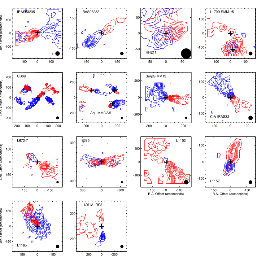
Figure 1.— Integrated intensity contours showing blueshifted and redshifted emission for the 17 outflows mapped in ¹²CO (2–1). Each panel is labeled with the name(s) of the source(s). The minimum and maximum velocities over which the emission is integrated are symmetrical about the rest velocity, and are chosen based on visual inspection of the velocity channels (see §3.2). In each panel we plot eight contour levels linearly spaced between three times the rms noise in each image and the maximum; the minimum contour and contour spacing are listed in Table 4. The driving sources are marked with crosses and the beam sizes are shown as black ellipses in the lower right of each panel.

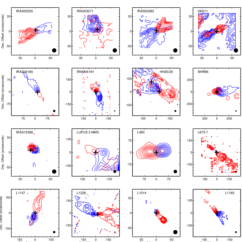
Figure 2.— Integrated intensity contours showing blueshifted and redshifted emission for the 17 outflows mapped in ¹²CO (3–2). Each panel is labeled with the name(s) of the source(s). The minimum and maximum velocities over which the emission is integrated are symmetrical about the rest velocity, and are chosen based on visual inspection of the velocity channels (see §3.2). In each panel we plot eight contour levels linearly spaced between three times the rms noise in each image and the maximum; the minimum contour and contour spacing are listed in Table 4. The driving sources are marked with crosses and the beam sizes are shown as black ellipses in the lower right of each panel.

2.4. Data Reduction

Low-order polynomial baselines were subtracted from all of the raw data using the default software package for each telescope: Continuum and Line Analysis Single-dish Software (CLASS) for APEX, CSO, SRAO, and SMT, NEWSTAR for ASTE, and Starlink for the JCMT. These packages were then used to combine together all observations of a particular source and write out FITS datacubes on grids of Nyquist sampled spatial pixels. Further analysis was performed using custom IDL procedures.

3. Results

Table 4Integrated Intensity Contour Levels for Figures 1 and 2

	Minimum Contour Level	Contour Step
Source	(K km s-1)	(K km s-1)
12CO (2–1) (Figure 1)
IRAS 03235$+$3004	0.60	0.51
IRAS 03282$+$3035	1.77	3.60
HH211	0.54	0.47
L1709-SMM1	1.12	1.27
L1709-SMM5	1.12	1.27
CB68	0.69	0.13
Aqu-MM2	2.81	2.16
Aqu-MM3	2.81	2.16
Aqu-MM5	2.81	2.16
SerpS-MM13	2.72	2.68
CrA-IRAS32	1.40	0.60
L673-7	0.80	0.94
B335	0.65	0.95
L1152	0.42	0.23
L1157	1.97	5.76
L1165	0.42	0.14
L1251A-IRS3	0.12	0.57
12CO (3–2) (Figure 2)
IRAS 03235$+$3004	0.35	0.36
IRAS 03271$+$3013	0.77	1.03
IRAS 03282$+$3035	2.90	2.46
HH211	1.53	0.56
IRAS 04166$+$2706	0.48	0.59
IRAM 04191$+$1522	1.70	2.42
HH25	3.29	12.57
HH26	3.29	12.57
BHR86	0.80	1.02
IRAS 15398$-$3359	0.90	1.09
Lupus 3 MMS	0.57	0.90
L483	0.27	0.17
L673-7	0.87	0.32
L1157	3.83	10.21
L1228	4.35	7.86
L1014	0.20	0.05
L1165	0.78	0.44

Figures 1 and 2 present integrated redshifted and blueshifted emission for each of the outflows mapped in ¹²CO (2–1) and ¹²CO (3–2), respectively, with the contour levels listed in Table 4. The minimum and maximum velocities over which the emission is integrated are symmetrical about the rest velocity for the redshifted and blueshifted emission, and are chosen based on visual inspection of the velocity channels (see §3.2). As is evident from these Figures, we detect outflows from all of our targets. While most of these outflows have been mapped by previous authors (see Appendix A), our results presented here represent the first complete molecular outflow maps published in the literature for Lupus 3 MMS, CrA-IRAS32, and L1152, and the first detection of the L1014 molecular outflow with a single-dish facility.

3.1. Outflow Geometrical Properties

Table 5Outflow Geometrical Properties

	$R_{\rm lobe}$	P.A.
Source	(AU)	(degrees)
12CO (2–1)
IRAS 03235$+$3004	$\geq$4.5${}\times 10^{4}$	107
IRAS 03282$+$3035	6.1${}\times 10^{4}$	126
HH211	1.5${}\times 10^{4}$	125
L1709-SMM1	1.6${}\times 10^{4}$	70
L1709-SMM5	$\cdots$	$\cdots$
CB68	2.3${}\times 10^{4}$	135
Aqu-MM2	2.3${}\times 10^{4}$	45
Aqu-MM3	3.0${}\times 10^{4}$	107
Aqu-MM5	5.5${}\times 10^{4}$	77
SerpS-MM13	$\geq$7.9${}\times 10^{4}$	78
CrA-IRAS32	2.1${}\times 10^{4}$	45
L673-7	4.5${}\times 10^{4}$	54
B335	4.9${}\times 10^{4}$	95
L1152	$\geq$6.9${}\times 10^{4}$	35
L1157	5.5${}\times 10^{4}$	160
L1165	6.0${}\times 10^{4}$	45
L1251A-IRS3	7.6${}\times 10^{4}$	5
12CO (3–2)
IRAS 03235$+$3004	$\geq$1.4${}\times 10^{4}$	115
IRAS 03271$+$3013	$\geq$1.4${}\times 10^{4}$	45
IRAS 03282$+$3035	$\geq$1.4${}\times 10^{4}$	115
HH211	1.4${}\times 10^{4}$	126
IRAS 04166$+$2706	1.5${}\times 10^{4}$	40
IRAM 04191$+$1522	2.2${}\times 10^{4}$	22
HH25	2.2${}\times 10^{4}$	155
HH26	6.2${}\times 10^{4}$	75
BHR86	4.0${}\times 10^{4}$	90
IRAS 15398$-$3359	3.0${}\times 10^{3}$	58
Lupus 3 MMS	2.1${}\times 10^{4}$	81
L483	2.2${}\times 10^{4}$	93
L673-7	5.5${}\times 10^{4}$	53
L1157	5.2${}\times 10^{4}$	160
L1228	6.1${}\times 10^{4}$	60
L1014	1.5${}\times 10^{4}$	45
L1165	3.8${}\times 10^{4}$	45

We measure and tabulate two geometrical properties of each outflow in Table 5: the average length of each outflow and the outflow position angle. The lobe length is measured by hand with a ruler using the integrated intensity contour maps presented in Figures 1 and 2, and the value reported in Table 5 is the mean of the red and blue lobes. The position angle is measured by hand with a protractor as the angle east of north, also using Figures 1 and 2. We estimate a typical measurement uncertainty of $\sim$2500 AU for the lobe length and $\sim$5^∘ for the position angle, and we list lower limits for the lobe lengths for outflows that clearly extend beyond the edges of our maps. We do not report values for either quantity for L1709-SMM2 due to the apparent pole-on geometry of this outflow, as inferred from the integrated intensity map.

With the relatively low spatial resolution of our single dish data, several outflows are either unresolved in width (direction perpendicular to the outflow axis) or only marginally resolved. As a consequence we do not report opening angles for the outflows since many such measurements would be biased to larger angles. Measurements of opening angles are better suited to interferometer studies of outflows, where the spatial resolution is high enough in most cases to resolve the outflows both along and perpendicular to their axes (e.g., Arce & Sargent, 2006).

3.2. Outflow Masses and Dynamical Properties

We calculate the masses of the outflows, $M_{\rm flow}$, and their dynamic properties (momentum, $P_{\rm flow}$, kinetic energy, $E_{\rm flow}$, luminosity, $L_{\rm flow}$, and force, $F_{\rm flow}$). For each outflow, we first calculate the column density of H₂, $N_{\mathrm{H_{2}}}$, within each velocity channel in each pixel. Since some maps contain multiple outflows and most maps have increased noise near their edges, we only consider spatial pixels within regions drawn to encompass the outflow lobes. Assuming optically thin, LTE emission, $N_{\mathrm{H_{2}}}=f(J,T_{\rm ex},X_{\rm CO})(\int\mbox{$T_{\rm mb}$}\,\mathrm{d}$$v)$, where $f(J,T_{\rm ex},X_{\rm CO})$ is a function of the quantum number of the lower state, $J$, the excitation temperature of the outflowing gas, $T_{\rm ex}$, and the CO abundance relative to H₂, $X_{\rm CO}$ (see Appendix C). The assumed excitation temperature is 50 K and is discussed in §4.2 below. The integral $\int\mbox{$T_{\rm mb}$}\,\mathrm{d}$$v$ is over the velocity channel and is given by the main-beam temperature in that channel multipled by the channel width. We assume a standard CO abundance relative to H₂ of $X_{\rm CO}=10^{-4}$, which is generally uncertain to within about a factor of three (e.g., Frerking et al., 1982; Lacy et al., 1994; Hatchell et al., 2007a).

Table 6Uncorrected Outflow Dynamical Properties

	$v_{\rm min}$	$v_{\rm max}$	$M_{\rm flow}$	$P_{\rm flow}$	$E_{\rm flow}$	$\tau_{\rm d}$	$L_{\rm flow}$	$F_{\rm flow}$
Source	(km s-1)	(km s-1)	(M⊙)	(M⊙ km s-1)	(ergs)	(yr)	(L⊙)	(M⊙ km s-1 yr-1)
12CO (2–1)
IRAS 03235$+$3004	2.0	4.5	$\geq$1.1${}\times 10^{-2}$	$\geq$2.7${}\times 10^{-2}$	$\geq$7.2${}\times 10^{41}$	4.7${}\times 10^{4}$	1.3${}\times 10^{-4}$	5.7${}\times 10^{-7}$
IRAS 03282$+$3035	6.0	19.0	4.7${}\times 10^{-2}$	4.3${}\times 10^{-1}$	4.3${}\times 10^{43}$	1.5${}\times 10^{4}$	2.3${}\times 10^{-2}$	2.8${}\times 10^{-5}$
HH211	2.9	6.0	2.8${}\times 10^{-3}$	1.0${}\times 10^{-2}$	4.0${}\times 10^{41}$	1.2${}\times 10^{4}$	2.8${}\times 10^{-4}$	8.7${}\times 10^{-7}$
L1709-SMM1	1.5	2.3	9.1${}\times 10^{-4}$	1.6${}\times 10^{-3}$	2.7${}\times 10^{40}$	3.3${}\times 10^{4}$	6.8${}\times 10^{-6}$	4.7${}\times 10^{-8}$
L1709-SMM5	2.0	5.1	$\geq$7.8${}\times 10^{-3}$	$\geq$2.3${}\times 10^{-2}$	$\geq$6.9${}\times 10^{41}$	$\cdots$	$\cdots$	$\cdots$
CB68	1.0	1.6	6.4${}\times 10^{-4}$	7.6${}\times 10^{-4}$	9.2${}\times 10^{39}$	6.8${}\times 10^{4}$	1.1${}\times 10^{-6}$	1.1${}\times 10^{-8}$
Aqu-MM2	3.0	9.6	1.4${}\times 10^{-2}$	6.9${}\times 10^{-2}$	3.7${}\times 10^{42}$	1.1${}\times 10^{4}$	2.7${}\times 10^{-3}$	6.0${}\times 10^{-6}$
Aqu-MM3	3.0	7.1	3.3${}\times 10^{-2}$	1.5${}\times 10^{-1}$	6.7${}\times 10^{42}$	2.0${}\times 10^{4}$	2.8${}\times 10^{-3}$	7.3${}\times 10^{-6}$
Aqu-MM5	3.0	7.4	6.5${}\times 10^{-3}$	2.6${}\times 10^{-2}$	1.1${}\times 10^{42}$	3.5${}\times 10^{4}$	2.5${}\times 10^{-4}$	7.3${}\times 10^{-7}$
SerpS-MM13	5.5	13.0	$\geq$7.4${}\times 10^{-2}$	$\geq$5.3${}\times 10^{-1}$	$\geq$4.0${}\times 10^{43}$	2.9${}\times 10^{4}$	1.1${}\times 10^{-2}$	1.8${}\times 10^{-5}$
CrA-IRAS32	2.0	3.8	1.6${}\times 10^{-3}$	3.8${}\times 10^{-3}$	9.5${}\times 10^{40}$	2.6${}\times 10^{4}$	3.0${}\times 10^{-5}$	1.5${}\times 10^{-7}$
L673-7	3.0	7.5	2.0${}\times 10^{-2}$	7.8${}\times 10^{-2}$	3.2${}\times 10^{42}$	2.8${}\times 10^{4}$	9.3${}\times 10^{-4}$	2.7${}\times 10^{-6}$
B335	1.0	5.5	1.5${}\times 10^{-2}$	2.9${}\times 10^{-2}$	6.6${}\times 10^{41}$	4.2${}\times 10^{4}$	1.3${}\times 10^{-4}$	6.9${}\times 10^{-7}$
L1152	2.0	3.5	$\geq$1.4${}\times 10^{-2}$	$\geq$3.3${}\times 10^{-2}$	$\geq$7.6${}\times 10^{41}$	9.4${}\times 10^{4}$	6.7${}\times 10^{-5}$	3.5${}\times 10^{-7}$
L1157	2.0	22.0	1.4${}\times 10^{-1}$	9.4${}\times 10^{-1}$	8.7${}\times 10^{43}$	1.2${}\times 10^{4}$	6.1${}\times 10^{-2}$	7.9${}\times 10^{-5}$
L1165	2.0	3.0	8.9${}\times 10^{-3}$	2.1${}\times 10^{-2}$	5.1${}\times 10^{41}$	9.5${}\times 10^{4}$	4.4${}\times 10^{-5}$	2.2${}\times 10^{-7}$
L1251A-IRS3	2.3	5.3	2.6${}\times 10^{-2}$	8.7${}\times 10^{-2}$	3.0${}\times 10^{42}$	6.8${}\times 10^{4}$	3.6${}\times 10^{-4}$	1.3${}\times 10^{-6}$
12CO (3–2)
IRAS 03235$+$3004	2.6	4.3	$\geq$4.4${}\times 10^{-4}$	$\geq$1.4${}\times 10^{-3}$	$\geq$4.6${}\times 10^{40}$	1.5${}\times 10^{4}$	2.5${}\times 10^{-5}$	9.1${}\times 10^{-8}$
IRAS 03271$+$3013	1.8	4.9	$\geq$1.8${}\times 10^{-3}$	$\geq$4.9${}\times 10^{-3}$	$\geq$1.4${}\times 10^{41}$	1.4${}\times 10^{4}$	8.6${}\times 10^{-5}$	3.6${}\times 10^{-7}$
IRAS 03282$+$3035	3.0	9.9	$\geq$9.3${}\times 10^{-3}$	$\geq$4.4${}\times 10^{-2}$	$\geq$2.2${}\times 10^{42}$	6.7${}\times 10^{3}$	2.7${}\times 10^{-3}$	6.5${}\times 10^{-6}$
HH211	2.0	2.7	9.4${}\times 10^{-4}$	2.1${}\times 10^{-3}$	4.9${}\times 10^{40}$	2.5${}\times 10^{4}$	1.7${}\times 10^{-5}$	8.7${}\times 10^{-8}$
IRAS 04166$+$2706	2.0	2.5	3.1${}\times 10^{-4}$	7.1${}\times 10^{-4}$	1.7${}\times 10^{40}$	2.0${}\times 10^{4}$	4.8${}\times 10^{-6}$	2.5${}\times 10^{-8}$
IRAM 04191$+$1522	2.0	7.7	5.4${}\times 10^{-3}$	1.8${}\times 10^{-2}$	6.8${}\times 10^{41}$	1.4${}\times 10^{4}$	4.2${}\times 10^{-4}$	1.3${}\times 10^{-6}$
HH25	4.0	10.5	1.8${}\times 10^{-2}$	8.5${}\times 10^{-2}$	4.5${}\times 10^{42}$	9.9${}\times 10^{3}$	3.7${}\times 10^{-3}$	8.5${}\times 10^{-6}$
HH26	4.0	24.5	2.7${}\times 10^{-1}$	2.0${}\times 10^{0}$	1.8${}\times 10^{44}$	1.2${}\times 10^{4}$	1.3${}\times 10^{-1}$	1.6${}\times 10^{-4}$
BHR86	2.0	5.6	1.3${}\times 10^{-2}$	3.7${}\times 10^{-2}$	1.1${}\times 10^{42}$	3.4${}\times 10^{4}$	2.7${}\times 10^{-4}$	1.1${}\times 10^{-6}$
IRAS 15398$-$3359	2.0	4.9	1.9${}\times 10^{-4}$	5.9${}\times 10^{-4}$	1.9${}\times 10^{40}$	2.9${}\times 10^{3}$	5.3${}\times 10^{-5}$	2.0${}\times 10^{-7}$
Lupus 3 MMS	2.0	4.0	1.7${}\times 10^{-3}$	4.4${}\times 10^{-3}$	1.1${}\times 10^{41}$	2.5${}\times 10^{4}$	3.8${}\times 10^{-5}$	1.8${}\times 10^{-7}$
L483	5.3	8.9	1.2${}\times 10^{-3}$	8.0${}\times 10^{-3}$	5.3${}\times 10^{41}$	1.2${}\times 10^{4}$	3.8${}\times 10^{-4}$	6.8${}\times 10^{-7}$
L673-7	2.0	3.6	4.0${}\times 10^{-3}$	9.4${}\times 10^{-3}$	2.3${}\times 10^{41}$	7.2${}\times 10^{4}$	2.6${}\times 10^{-5}$	1.3${}\times 10^{-7}$
L1157	1.4	8.3	4.0${}\times 10^{-2}$	1.3${}\times 10^{-1}$	5.0${}\times 10^{42}$	3.0${}\times 10^{4}$	1.4${}\times 10^{-3}$	4.3${}\times 10^{-6}$
L1228	2.0	12.0	6.7${}\times 10^{-2}$	2.7${}\times 10^{-1}$	1.3${}\times 10^{43}$	2.4${}\times 10^{4}$	4.4${}\times 10^{-3}$	1.1${}\times 10^{-5}$
L1014	1.3	3.0	9.3${}\times 10^{-5}$	1.7${}\times 10^{-4}$	3.1${}\times 10^{39}$	2.4${}\times 10^{4}$	1.1${}\times 10^{-6}$	7.2${}\times 10^{-9}$
L1165	1.6	4.0	2.4${}\times 10^{-3}$	5.9${}\times 10^{-3}$	1.5${}\times 10^{41}$	4.5${}\times 10^{4}$	2.8${}\times 10^{-5}$	1.3${}\times 10^{-7}$

The mass within each velocity channel in each pixel is then calculated as $M_{\rm v,pixel}=\mu_{\rm H_{2}}m_{\rm H}N_{\mathrm{H_{2}}}A_{\rm pixel}$, where $m_{\rm H}$ is the mass of a hydrogen atom, $\mu_{\rm H_{2}}$ is the mean molecular weight per hydrogen molecule ($\mu_{\rm H_{2}}=2.8$ for gas composed of 71% hydrogen, 27% helium, and 2% metals by mass (Kauffmann et al., 2008)), and $A_{\rm pixel}$ is the area of each pixel. The total mass of each outflow is then obtained by summing $M_{\rm v,pixel}$ over all velocity and spatial pixels encompassing the outflow. The velocities of integration are assumed to be symmetrical about the rest velocities and are chosen based on visual inspection of channel maps for each outflow. To determine the lower bound of integration, which we define as $v_{\rm min}$, we select the lowest-velocity redshifted and blueshifted channels where the ambient cloud emission drops below 3$\sigma$ (measured at locations outside of the outflow lobes to avoid issues with separating ambient cloud and outflow emission). Since we adopt symmetrical velocity limits for blueshifted and redshfited emission, the larger of these two (measured relative to rest) is then taken to be $v_{\rm min}$ and is listed in the second column of Table 6. To determine the upper bound of integration, which we define as $v_{\rm max}$, we select the highest-velocity redshifted and blueshifted channels where outflowing gas is detected above 3$\sigma$. The larger of these two (again, measured relative to rest) is taken to be $v_{\rm max}$ and is listed in the third column of Table 6. Average spectra for each outflow, with the ambient cloud velocity, $v_{\rm min}$, and $v_{\rm max}$ indicated, are shown in Appendix B.

Some ambient cloud emission is still apparent in Figures 1 and 2 since some of the channels above the lower bound contain ambient emission below 3$\sigma$ that integrates to levels above the 3$\sigma$ rms of the integrated maps. None of this ambient emission is included in our calculations of outflow masses and dynamical properties since we first cut out all emission below 3$\sigma$ in each velocity channel before calculating these properties. The calculated masses (assuming a temperature of 50 K; see §4.2) are listed in the fourth column of Table 6.

The momentum and kinetic energy within each velocity channel in each pixel are calculated as $P_{\rm v,pixel}=M_{\rm v,pixel}\times v$ and $E_{\rm v,pixel}=\frac{1}{2}M_{\rm v,pixel}\times v^{2}$, respectively, where $v$ is the velocity of each channel with respect to the systemic velocity. The total momentum ($P_{\rm flow}$) and kinetic energy ($E_{\rm flow}$) of each outflow are then calculated by summing over the same velocity and spatial pixels as for the mass, and are listed in the fifth and sixth columns of Table 6. Some authors instead define the total $P_{\rm flow}$ and $E_{\rm flow}$ as the total $M_{\rm flow}$ multiplied by ($v_{\rm char}$) or ($\frac{1}{2}v_{\rm char}^{2}$), respectively, where $v_{\rm char}$ is the intensity (or mass) weighted outflow velocity (e.g., Andre et al., 1990). Such a method is mathematically identical for $P_{\rm flow}$ but will underestimate the total $E_{\rm flow}$ since it will not fully account for the large fraction of total energy contained in the highest velocity gas. Finally, the luminosity and force of each outflow are calculated as $L_{\rm flow}$ $=$ $E_{\rm flow}$ $/$ $\tau_{\rm d}$ and $F_{\rm flow}$ $=$ $P_{\rm flow}$$/$ $\tau_{\rm d}$, respectively, where $\tau_{\rm d}$ is the dynamical time. It is calculated as $\tau_{\rm d}=R_{\rm lobe}/v_{\rm max}$, with $R_{\rm lobe}$ and $v_{\rm max}$ (the average length of the red and blue lobes and the maximum velocity at which outflowing gas is detected above 3$\sigma$, respectively) listed in Tables 5 and 6. The seventh, eighth, and ninth columns list $\tau_{\rm d}$, $L_{\rm flow}$, and $F_{\rm flow}$, respectively. Note that the dynamical time of an outflow likely underestimates its true age due to rapid acceleration and decelaration in the outflow (Parker et al., 1991; Masson & Chernin, 1992, 1993).

Inspection of Figures 1 and 2 clearly show that some outflows extend beyond the mapped areas. The values of $M_{\rm flow}$, $P_{\rm flow}$, and $E_{\rm flow}$ that we calculate for these outflows are thus lower limits and marked as such in Table 6. The calculated values of $L_{\rm flow}$ and $F_{\rm flow}$, however, are reliable measures of the total outflow luminosities and driving forces as long as the energy and momentum injection rates are assumed to be constant over the lifetime of the detectable outflow.

4. Correction Factors to Outflow Properties

In the above section, we calculated the masses and dynamical properties of the outflows studied here assuming optically thin, LTE emission at an excitation temperature of 50 K, and only integrating channels at velocities larger than those in which ambient cloud emission is detected. Below we attempt to quantify the correction factors that must be applied to the values obtained under these simple assumptions.

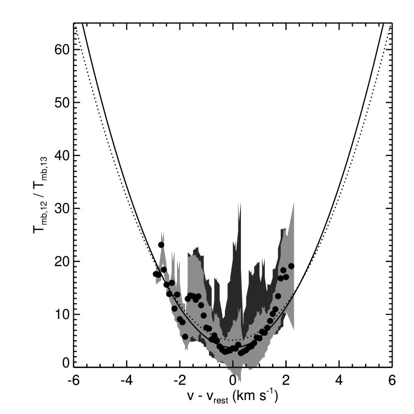
Figure 3.— $T_{\rm mb,12}/T_{\rm mb,13}$ as a function of velocity from rest for ¹²CO (2–1) and ¹³CO (2–1). Plotted are the mean ratio determined from all of the pointed observations (circles), the standard deviation at each velocity (light gray shading), the full extent at each velocity (dark gray shading), the best-fit second-order polynomial (solid black line), and the best-fit second-order polynomial after excluding all velocity channels with $|(v-v_{\rm rest})|<1$ km s^-1 (dotted line).

4.1. Opacity

Numerous studies have established that the line-wings of outflows are typically optically thick in low-J transitions of ¹²CO (e.g., Goldsmith et al., 1984; Cabrit & Bertout, 1992; Bally et al., 1999; Arce & Goodman, 2001; Curtis et al., 2010b). Using our ¹³CO data obtained as described above, we follow a standard method of correcting the outflow masses and dynamical properties (e.g., Goldsmith et al., 1984; Curtis et al., 2010b). Assuming that both ¹²CO and ¹³CO are in LTE at the same excitation temperature, and further assuming identical beam-filling factors, the ratio of brightness temperatures between the two isotopologues is given as

$$\frac{T_{\rm mb,12}}{T_{\rm mb,13}}=\frac{1-e^{-\tau_{12}}}{1-e^{-\tau_{13}}}\qquad,$$ (1)

where $T_{\rm mb,12}$ and $T_{\rm mb,13}$ are the observed ¹²CO and ¹³CO brightness temperatures, respectively, and $\tau_{12}$ and $\tau_{13}$ are the opacities of the ¹²CO and ¹³CO transitions. Assuming that the ¹³CO is optically thin, Equation 1 can be rewritten as

$$\frac{T_{\rm mb,12}}{T_{\rm mb,13}}=\frac{[^{12}\rm{CO}]}{[^{13}\rm{CO}]}\frac{1-e^{-\tau_{12}}}{\tau_{12}}\qquad,$$ (2)

where $[^{12}\rm{CO}]/[^{13}\rm{CO}]$ is the abundance ratio, which is taken to be 62 (Langer & Penzias, 1993). Using this expression, $\tau_{12}$ can be determined numerically from the observed ratio $T_{\rm mb,12}/T_{\rm mb,13}$, and then the correction factor $\tau_{12}/(1-e^{-\tau_{12}})$ can be applied to the ¹²CO data to correct the observed brightness temperatures to the values they would have in the optically thin limit. As noted by Wilson et al. (2009), Equation 2 overestimates the ratio of brightness temperatures by an amount that increases with $\tau_{12}$, due to the increasingly invalid assumption that the ¹³CO is optically thin. The most optically thick outflows in our sample have $\tau_{12}\sim 10-20$ (as derived below), which leads to overestimates in Equation 2 of 5% – 15%. These overestimates are small enough to have no significant effect on our results.

4.1.1 $J=2-1$

Figure 4.— $T_{\rm mb,12}/T_{\rm mb,13}$ as a function of velocity from rest for ¹²CO (3–2) and ¹³CO (3–2). Left: Plotted are the mean ratio determined from all of the pointed observations (circles), the standard deviation at each velocity (light gray shading), the full extent at each velocity (dark gray shading), and the best-fit second-order polynomial (solid black line). Only ratios used in the polynomial fit are plotted (see text for details). Right: Plotted is the ratio determined from the average ¹²CO (3–2) and ¹³CO (3–2) L673-7 spectra (circles with error bars), and the best-fit second-order polynomial.

As listed in Table 3, we obtained pointed ¹³CO (2–1) observations toward 17 positions in five different outflows. To facilitate comparison between ¹²CO and ¹³CO, we also obtained pointed ¹²CO (2–1) observations toward these same positions on the same nights to remove uncertainties introduced by different telescope beams, efficiencies, and weather conditions. For each of these 17 positions, we calculate $T_{\rm mb,12}/T_{\rm mb,13}$ as a function of velocity measured relative to rest (such that the systemic core velocity is equal to 0 km s^-1) for each velocity where both lines are detected at or above 3$\sigma$.

Since we only have select pointed ¹³CO observations (obtaining full ¹³CO maps of multiple outflows to the depths required to detect line-wings from outflows is prohibitively expensive in terms of telescope time), we average each of the $T_{\rm mb,12}/T_{\rm mb,13}$ from above to obtain a mean ratio in each velocity bin. Following Arce & Goodman (2001), we then use linear least-squares to fit a second order polynomial to the mean ratio versus velocity, constrained to reach a minimum at rest (zero) velocity. This allows us to correct for opacity even at velocities where the line-wings were not detected in ¹³CO. For the fit we only consider velocities within $\pm$4 km s^-1 from rest that have two or more measurements of the ratio.

Table 7Outflow Correction Factors

	Opacity					Low-Velocity					Sensitivity
Source	$M_{\rm flow}$	$P_{\rm flow}$	$E_{\rm flow}$	$L_{\rm flow}$	$F_{\rm flow}$	$M_{\rm flow}$	$P_{\rm flow}$	$E_{\rm flow}$	$L_{\rm flow}$	$F_{\rm flow}$	$M_{\rm flow}$	$P_{\rm flow}$	$E_{\rm flow}$	$L_{\rm flow}$	$F_{\rm flow}$
12CO (2–1)
IRAS 03235$+$3004	4.2	4.1	3.9	3.8	4.2	6.7	4.4	2.9	2.8	4.3	1.6	1.6	1.6	1.8	1.8
IRAS 03282$+$3035	1.0	1.0	1.0	1.0	1.0	7.6	3.8	2.1	2.2	3.8	1.2	1.3	1.5	2.0	1.8
HH211	2.4	2.4	2.1	2.1	2.3	14.4	8.0	4.7	4.7	8.1	1.1	1.2	1.4	2.4	2.1
L1709-SMM1	7.3	6.9	7.0	7.1	7.2	$\cdots$	$\cdots$	$\cdots$	$\cdots$	$\cdots$	1.3	1.4	1.4	1.4	1.4
L1709-SMM2	3.8	3.5	3.2	$\cdots$	$\cdots$	1.6	1.3	1.2	$\cdots$	$\cdots$	1.2	1.2	1.2	$\cdots$	$\cdots$
CB68	10.6	10.5	10.3	10.0	10.9	$\cdots$	$\cdots$	$\cdots$	$\cdots$	$\cdots$	2.4	2.3	2.2	2.9	2.8
Aqu-MM2	1.6	1.4	1.4	1.4	1.5	$\cdots$	$\cdots$	$\cdots$	$\cdots$	$\cdots$	1.3	1.4	1.3	1.4	1.3
Aqu-MM3	1.7	1.6	1.6	1.6	1.6	2.6	1.8	1.3	1.3	1.7	1.1	1.2	1.1	1.5	1.5
Aqu-MM5	2.2	2.0	1.9	1.9	2.1	9.2	5.0	2.9	3.0	5.0	1.4	1.5	1.5	2.1	2.0
SerpS-MM13	1.0	1.0	1.0	1.0	1.0	$\cdots$	$\cdots$	$\cdots$	$\cdots$	$\cdots$	1.2	1.2	1.3	1.5	1.3
CrA-IRAS32	4.6	4.5	4.4	4.3	4.4	$\cdots$	$\cdots$	$\cdots$	$\cdots$	$\cdots$	1.5	1.6	1.6	2.0	1.8
L673-7	2.3	2.2	2.0	1.9	2.1	$\cdots$	$\cdots$	$\cdots$	$\cdots$	$\cdots$	1.2	1.2	1.2	1.3	1.3
B335	6.6	5.9	5.0	4.9	5.8	$\cdots$	$\cdots$	$\cdots$	$\cdots$	$\cdots$	$\cdots$	$\cdots$	$\cdots$	$\cdots$	$\cdots$
L1152	5.1	4.8	4.7	4.8	4.9	7.0	4.7	3.3	3.4	4.8	1.5	1.6	1.6	2.2	2.1
L1157	2.2	1.5	1.1	1.2	1.5	1.8	1.2	1.1	1.0	1.2	1.1	1.1	1.4	1.5	1.3
L1165	4.8	4.8	4.5	4.5	4.5	2.5	1.9	1.6	1.6	2.0	1.5	1.6	1.7	2.1	2.1
L1251A-IRS3	3.1	2.8	2.6	2.6	2.8	$\cdots$	$\cdots$	$\cdots$	$\cdots$	$\cdots$	1.4	1.4	1.4	1.4	1.4
12CO (3–2)
IRAS 03235$+$3004	2.5	2.5	2.4	2.4	2.4	$\cdots$	$\cdots$	$\cdots$	$\cdots$	$\cdots$	1.0	1.0	1.2	1.6	1.4
IRAS 03271$+$3013	2.0	1.8	1.6	1.5	1.8	5.0	3.7	2.8	2.9	3.7	1.0	1.1	1.3	1.7	1.3
IRAS 03282$+$3035	1.0	1.0	1.0	1.0	1.0	5.5	3.1	2.0	1.9	3.1	1.3	1.4	1.6	2.2	2.0
HH211	2.1	2.2	2.0	2.1	2.2	12.9	9.6	7.7	7.4	9.5	2.2	2.6	3.4	5.7	4.5
IRAS 04166$+$2706	2.1	2.1	2.0	2.1	2.1	$\cdots$	$\cdots$	$\cdots$	$\cdots$	$\cdots$	$\cdots$	$\cdots$	$\cdots$	$\cdots$	$\cdots$
IRAM 04191$+$1522	1.4	1.3	1.2	1.2	1.4	5.6	3.5	2.4	2.4	3.5	$\cdots$	$\cdots$	$\cdots$	$\cdots$	$\cdots$
HH25	1.0	1.0	1.0	1.0	1.0	$\cdots$	$\cdots$	$\cdots$	$\cdots$	$\cdots$	$\cdots$	$\cdots$	$\cdots$	$\cdots$	$\cdots$
HH26	1.0	1.0	1.0	1.0	1.0	$\cdots$	$\cdots$	$\cdots$	$\cdots$	$\cdots$	$\cdots$	$\cdots$	$\cdots$	$\cdots$	$\cdots$
BHR86	1.8	1.6	1.5	1.5	1.6	6.0	4.1	3.1	3.0	4.0	$\cdots$	$\cdots$	$\cdots$	$\cdots$	$\cdots$
IRAS 15398$-$3359	1.5	1.4	1.3	1.3	1.4	$\cdots$	$\cdots$	$\cdots$	$\cdots$	$\cdots$	1.3	1.4	1.5	1.7	1.6
Lupus 3 MMS	2.0	1.8	1.8	1.7	1.8	9.2	6.0	4.1	4.2	6.0	$\cdots$	$\cdots$	$\cdots$	$\cdots$	$\cdots$
L483	1.0	1.0	1.0	1.0	1.0	23.1	13.2	7.0	6.9	13.2	$\cdots$	$\cdots$	$\cdots$	$\cdots$	$\cdots$
L673-7	2.1	2.0	1.9	1.9	2.0	$\cdots$	$\cdots$	$\cdots$	$\cdots$	$\cdots$	1.2	1.4	1.6	2.4	2.1
L1157	2.1	1.5	1.3	1.3	1.6	$\cdots$	$\cdots$	$\cdots$	$\cdots$	$\cdots$	1.8	2.8	5.8	14.4	6.8
L1228	1.3	1.2	1.1	1.1	1.2	$\cdots$	$\cdots$	$\cdots$	$\cdots$	$\cdots$	$\cdots$	$\cdots$	$\cdots$	$\cdots$	$\cdots$
L1014	3.3	3.3	3.2	3.2	3.2	$\cdots$	$\cdots$	$\cdots$	$\cdots$	$\cdots$	$\cdots$	$\cdots$	$\cdots$	$\cdots$	$\cdots$
L1165	2.2	2.0	1.8	1.8	2.0	10.8	7.0	5.1	5.1	7.2	$\cdots$	$\cdots$	$\cdots$	$\cdots$	$\cdots$
Mean	2.8	2.6	2.5	2.4	2.6	7.7	4.8	3.3	3.4	5.1	1.4	1.5	1.7	2.6	2.1
Median	2.1	2.0	1.8	1.7	1.8	6.7	4.1	2.9	3.0	4.3	1.3	1.4	1.5	2.0	1.8
Minimum	1.0	1.0	1.0	1.0	1.0	1.6	1.2	1.0	1.0	1.2	1.0	1.0	1.1	1.3	1.3
Maximum	10.6	10.5	10.3	10.0	10.9	23.1	13.2	7.7	7.4	13.2	2.4	2.8	5.8	14.4	6.8

Figure 3 plots the mean $T_{\rm mb,12}/T_{\rm mb,13}$ as a function of velocity from rest for all points used in the fit, as well as the resulting second-order polynomial fit. The fit is described by the equation

$$T_{\rm mb,12}/T_{\rm mb,13}=(1.90\pm 0.09)\,(\rm{v-v_{rest}})^{2}+(3.72\pm 0.48)\,,$$ (3)

and has a reduced $\chi^{2}$ of 0.53. Since it is possible that the lowest velocity channels are optically thick even in ¹³CO, we also repeated the fit after excluding all channels where $|(v-v_{\rm rest})|<1$ km s^-1. The resulting fit is also plotted in Figure 3 and is within the uncertainties of the original fit and thus has no significant effect on our results. To correct all of our ¹²CO (2–1) data for opacity, we take, at each velocity, the smaller of either the polynomial fit or 62 (the abundance ratio), use this value to calculate $\tau_{12}$ at each velocity numerically using Equation 2, and then apply the velocity-dependent correction factor $\tau_{12}/(1-e^{-\tau_{12}})$ to our data.

4.1.2 $J=3-2$

We obtained pointed ¹³CO (3–2) observations toward five positions in three different outflows, again with corresponding pointed ¹²CO (3–2) observations to facilitie comparison between the two isotopologues. The decreased number of positions in the 3–2 transition (five) compared to the 2–1 transition (17) was due to less available time in the required weather conditions. As above, we average the results from each pointed observation to determine a mean $T_{\rm mb,12}/T_{\rm mb,13}$ for each velocity, and then fit a second-order polynomial, constrained to reach its minimum at rest (zero) velocity, to all velocities within $\pm$4 km s^-1 from rest that have two or more individual measurements of $T_{\rm mb,12}/T_{\rm mb,13}$. The resulting mean $T_{\rm mb,12}/T_{\rm mb,13}$ and best-fit polynomial are shown in the left panel of Figure 4. The fit is described by the equation

$$I_{12}/I_{13}=(2.50\pm 0.55)\,(\rm{v-v_{rest}})^{2}+(1.87\pm 0.27)\,,$$ (4)

and has a reduced $\chi^{2}$ of 0.27.

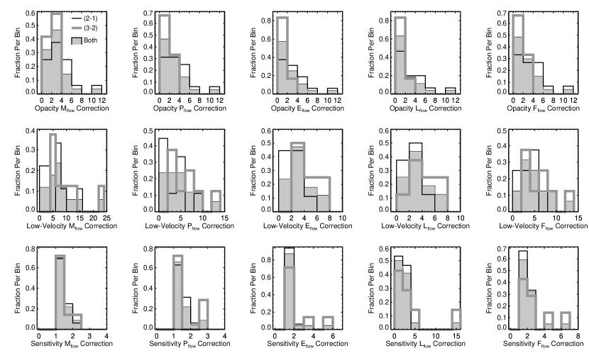
Figure 5.— Histograms showing the distributions of correction factors listed in Table 7. The top panels show the corrections for opacity, the middle panels show the corrections for low-velocity emission, and the bottom panels show the corrections for sensitivity. From left-to-right, the panels plot the corrections for $M_{\rm flow}$, $P_{\rm flow}$, $E_{\rm flow}$, $L_{\rm flow}$, and $F_{\rm flow}$. The thin black histogram plots the corrections derived for the outflows mapped in ¹²CO (2–1), the thick gray histogram plots those derived for the outflows mapped in ¹²CO (3–2), and the shaded histograms show the combined sample.

Given that only five pointings went into deriving this fit, we caution that it is extremely uncertain. Indeed, inspection of Figure 4 shows that it is not even clear if a second-order polynomial is an approriate function to fit, and even if it is the fit is certainly not very well constrained. As noted above, we also obtained a ¹³CO (3–2) map of the full extent of the L673-7 outflow. This map is not sensitive enough for robust line-wing detection at each spatial position, thus instead we calculate the average ¹²CO (3–2) and ¹³CO (3–2) spectrum over all spatial pixels that encompass the outflow. We calculate the ratio $T_{\rm mb,12}/T_{\rm mb,13}$ as a function of velocity from these average spectra for all velocities where both spectra are detected at or above 3$\sigma$, and again fit a second-order polynomial constrained to reach its minimum at rest (zero) velocity. This fit is described by the equation

$$T_{\rm mb,12}/T_{\rm mb,13}=(5.77\pm 0.68)\,(\rm{v-v_{rest}})^{2}+(1.73\pm 0.03)\,,$$ (5)

and has a reduced $\chi^{2}$ of 0.48. The observed $T_{\rm mb,12}/T_{\rm mb,13}$ and best-fit polynomial are shown in the right panel of Figure 4.

We choose to use the fit to $T_{\rm mb,12}/T_{\rm mb,13}$ determined from L673-7 to determine opacity corrections for our ¹²CO (3–2) data because of the increased redundancy in using an entire outflow rather than only five pointings in three different outflows, and also because it is much clearer in this case that a second-order polynomial provides a good fit to the data. The procedure for using the fit to derive velocity-dependent opacity corrections is the same as above for ¹²CO (2–1), except now using the L673-7 polynomial fit. Since the L673-7 outflow is a relatively low-mass outflow compared to several others considered in this study and thus may be less optically thick, we caution that our results may underestimate the magnitude of the opacity corrections for some of the more massive outflows mapped in ¹²CO (3–2).

4.1.3 Opacity Corrections

Columns two through six of Table 7 list the resulting factors by which $M_{\rm flow}$, $P_{\rm flow}$, $E_{\rm flow}$, $L_{\rm flow}$, and $F_{\rm flow}$ increase when these opacity corrections are applied, and the top row of Figure 5 shows the distribution of opacity correction factors separately for the outflows mapped in each transition and combined. For the combined sample, we find that the outflow mass is increased by factors ranging from 1.0 to 10.6, with a mean (median) increase of 2.8 (2.1), and similar increases for the other properties. Using a similar procedure for outflows in Perseus mapped in ¹²CO (3–2), Curtis et al. (2010b) found that their outflow masses increase by factors ranging from 1.8 to 14.3, with a median of 3.8. Additionally, Cabrit & Bertout (1992) found opacity corrections ranging from 1.0 to 8.9, with a mean of 3.5, using a simpler method that applied one correction factor at all velocities. In both cases our results are comparable.

Both our results and previous studies (e.g., Cabrit & Bertout, 1992; Curtis et al., 2010b) find a range in opacity correction factors of approximately one order of magnitude. Since the velocity-dependent opacity corrections are largest at the lowest velocities where the emission is the most optically thick, the magnitude of the total correction is expected to depend on the lower bound of the velocity range used to calculate the outflow properties. As confirmed by the left panel of Figure 6, most of the range in total opacity correction factors is indeed explained by such a trend. This trend likely explains why van der Marel et al. (2013) concluded that opacity corrections are less than a factor of two and can thus be neglected, since their minimum velocities were typically $\sim$3 km s^-1.

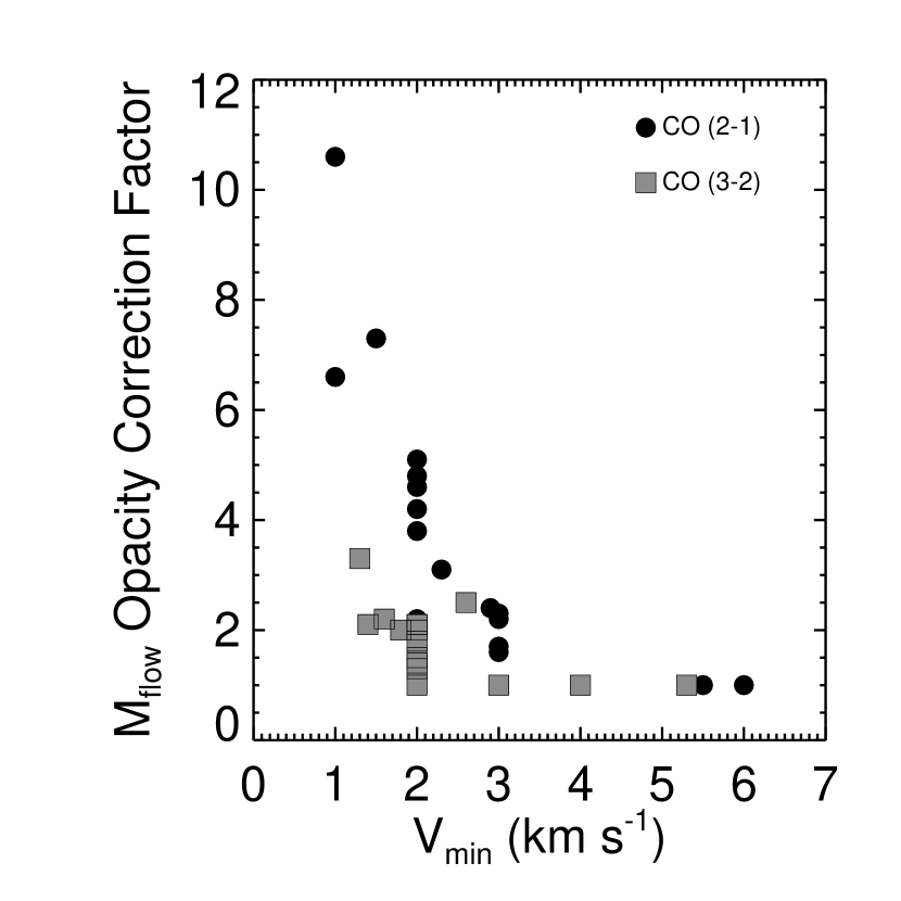
Figure 6.— Left: Total opacity correction factor for $M_{\rm flow}$ plotted vs. the lower bound of the velocity range used to calculate the outflow properties, taken from Table 6. Black circles show the corrections for outflows mapped in ¹²CO (2–1), and gray squares show the corrections for outflows mapped in ¹²CO (3–2). Similar trends are seen for the other outflow dynamical properties ($P_{\rm flow}$, $E_{\rm flow}$, $L_{\rm flow}$, and $F_{\rm flow}$). Right: $T_{\rm mb,12}/T_{\rm mb,13}$ determined from observations of ¹²CO (2–1) and ¹³CO (2–1) toward one of the positions observed in the IRAS 03282$+$3035 outflow (circles), with the position labeled in the top center of the panel. The solid black line shows the best-fit second-order polynomial to the mean $T_{\rm mb,12}/T_{\rm mb,13}$ from all 17 pointed observations and is the same as that displayed in Figure 3.

Finally, we end this section by noting that there is some limited evidence that our method underestimates the opacity correction factors. As seen in Figures 3 and 4, the second-order polynomial fits to the observed $T_{\rm mb,12}/T_{\rm mb,13}$ reach the abundance ratio of 62, implying fully optically thin emission, for all velocities beyond $\sim$4–6 km s^-1 from rest. However, the right panel of Figure 6 plots the observed $T_{\rm mb,12}/T_{\rm mb,13}$ for the ¹²CO (2–1) and ¹³CO (2–1) observations of a position in the IRAS 03282$+$3035 outflow. This is one of the only set of pointed observations where ¹³CO is detected at or above 3$\sigma$ beyond 4 km s^-1 from rest, and in this case $T_{\rm mb,12}/T_{\rm mb,13}$ at these higher velocities is clearly below the fit, suggesting the emission is more optically thick at these velocities than predicted by the fit. ¹³CO observations with higher sensitivity than those presented here are required to test the generality of this result, and such observations should be possible in the near future with the Atacama Large Millimeter Array (ALMA) and the Cerro Chajnantor Atacama Telescope (CCAT).

4.2. Excitation Temperature

An unknown parameter in the calculation of $M_{\rm flow}$ (and all other dynamical properties that depend on mass) is $T_{\rm ex}$, the excitation temperature of the outflowing gas. Most studies adopt values of $T_{\rm ex}$ in the range of 10 – 50 K (e.g., Parker et al., 1991; Hatchell et al., 2007a; Curtis et al., 2010b; Dunham et al., 2010). However, van Kempen et al. (2009c, d) used multiple transitions of ¹²CO (up to (6–5)) to derive warmer temperatures, in the range of 50–200 K, for a sample of six outflows. Similarly high temperatures were found by Yıldız et al. (2013) with Herschel high-J ¹²CO observations up to ¹²CO (10–9).

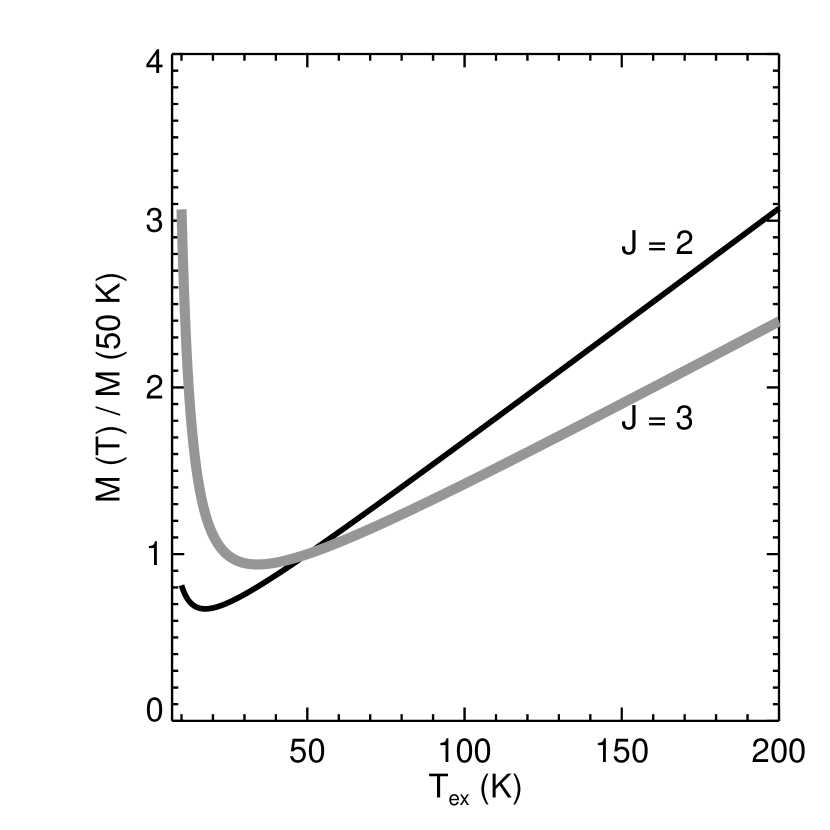
Figure 7.— Correction factors for outflow mass (and all other properties that depend on mass) for different assumed $T_{\rm ex}$, compared to the assumed value of 50 K. Correction factors for both ¹²CO (2–1) (black line) and ¹²CO (3–2) (gray line) are plotted. See Appendix C for details on the calculation.

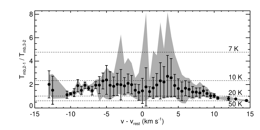
Figure 8.— The mean value of $T_{\rm mb,2-1}/T_{\rm mb,3-2}$ plotted versus velocity from rest for the six outflows mapped in both ¹²CO (2–1) and ¹²CO (3–2). The averages are calculated over 0.5 km s^-1 wide bins, with the standard deviation in each bin plotted as error bars and the total extent in each bin plotted as the gray shaded area. The line ratios for LTE temperatures of 7, 10, 20, and 50 K are marked with dotted lines.

Figure 7 shows the factors by which $M_{\rm flow}$ (and all other properties that depend on it) would change for $T_{\rm ex}=10-200$ K, relative to the assumed value of 50 K (see Appendix C for details on the calculation). These factors range from $0.7-3$, depending on transition and $T_{\rm ex}$. For both transitions, values above 50 K can only increase outflow properties, up to a factor of three compared to the assumption of $T_{\rm ex}=50$ K. Since we mapped six outflows (IRAS 03235$+$3004, IRAS 03282$+$3035, HH211, L673-7, L1157, and L1165) in both the (2–1) and (3–2) transitions of ¹²CO, here we use our data to study the excitation temperatures of these outflows.

For each of the six outflows, we corrected both transitions for opacity using our velocity-dependent corrections, re-gridded them onto the same velocity grid, convolved the ¹²CO (3–2) map with a Gaussian with a FWHM such that the output map matches the resolution of the ¹²CO (2–1) map, aligned the convolved ¹²CO (3–2) and original ¹²CO (2–1) maps onto the same spatial grid, calculated the mean spectra in each outflow lobe for each transition, and finally calculated $T_{\rm mb,2-1}/T_{\rm mb,3-2}$, the ratio of the mean spectra, for each lobe of each outflow.

Figure 8 displays the mean value of $T_{\rm mb,2-1}/T_{\rm mb,3-2}$ versus velocity from rest over all six outflows in 0.5 km s^-1 bins and shows that $T_{\rm mb,2-1}/T_{\rm mb,3-2}$ ranges between $\sim 0.5-3$. Assuming LTE, nearly all of the velocities are consistent with $T_{\rm ex}$ in the range of 10 – 20 K. While there is very weak evidence for higher $T_{\rm ex}$ (up to 50 K) at the highest redshifted velocities, in general there is no clear trend in $T_{\rm mb,2-1}/T_{\rm mb,3-2}$ (and thus in implied $T_{\rm ex}$) with velocity. In contrast, Yıldız et al. (2013) found clear evidence for increasing $T_{\rm ex}$ with velocity with higher-J Herschel observations of outflows.

Figure 9.— Expected $T_{\rm mb,2-1}/T_{\rm mb,3-2}$ plotted as a function of $T_{\rm ex}$, assuming LTE. See Appendix C for details on the calculation.

Our results seem to imply that the most appropriate assumptions for $T_{\rm ex}$ for the outflows studied here are those ranging from 10 to 20 K, which would lead to outflow properties that decrease by 20% – 30% for those mapped in ¹²CO (2–1) and increase by factors of 1 – 3 for those mapped in ¹²CO (3–2), compared to the values obtained by assuming $T_{\rm ex}=50$ K. However, we caution that, by only considering ¹²CO (2–1) and ¹²CO (3–2), we are not sensitive to the presence of gas with $T_{\rm ex}$ above $\sim 50$ K, as clearly demonstrated by Figure 9, which shows that the line ratios change by only $\sim 0.1$ for $T_{\rm ex}$ between 50 and 200 K. Higher-J transitions would be required to evaluate the existence of warmer gas. To further reinforce this point, we calculated the ratio $T_{\rm mb,2-1}/T_{\rm mb,3-2}$ assuming an equal-mass mixture of warm (200 K) and cold (either 10 K or 50 K) gas is observed (see Appendix C for details on the calculation, and note that, in the notation of Appendix C, $A=1$ for an equal-mass mixture of warm and cold gas). If the resulting ratios were then assumed to arise from gas in LTE at a single temperature, the derived $T_{\rm ex}$ are 15.5 K for the mixture with cold gas at 10 K, and 63 K for the mixture with cold gas at 50 K. The warm, 200 K gas is almost completely invisible in the analysis of the ratio of $T_{\rm mb,2-1}/T_{\rm mb,3-2}$.

Since van Kempen et al. (2009c, d) and Yıldız et al. (2013) found typical $T_{\rm ex}$ ranging from 50 to 200 K with higher-J transitions of ¹²CO, we adopt 50 K in this paper and note that our results may increase by up to factors of 3 if the temperatures are higher. In reality, the gas in molecular outflows may not all be at the same excitation temperature; there may be variations both spatially and kinematically, and there may be very warm molecular gas in shocks (e.g., Green et al., 2013; Yıldız et al., 2013; Santangelo et al., 2013). Indeed, Downes & Cabrit (2007) showed that the $T_{\rm ex}$ of their simulated outflows increased with increasing velocity, and Yıldız et al. (2013) found a similar trend in Herschel observations of low-mass protostars. Downes & Cabrit (2007) cautioned that using a single temperature can lead to significant underestimates (by up to factors of $3-4$) in the outflow kinetic energy and mechanical luminosity, since both quantities depend on the square of velocity and thus give the most weight to the highest-velocity gas. Since our data do not show any clear trend between $T_{\rm ex}$ and velocity, and are generally insensitive to the presence of gas above 50 K anyway, we are unable to evaluate the effects of such an underestimate on our calculated outflow properties.

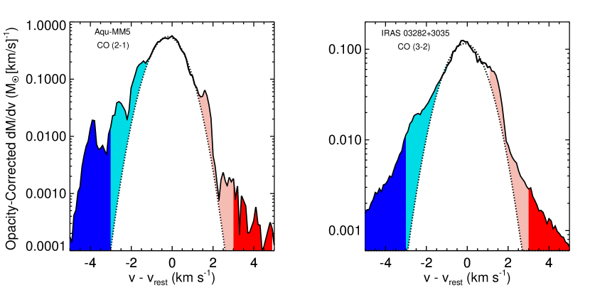
Figure 10.— Total mass spectra, $dM/dv$, for two outflows: Aqu-MM5 mapped in ¹²CO (2–1) (left) and IRAS 03282$+$3035 mapped in ¹²CO (3–2) (right). The mass spectra are calculated by summing the mass in each velocity channel (corrected for opacity using the velocity-dependent corrections derived in §4.1) over the total extent of the outflow, and are plotted as solid black lines. The dotted lines show the Gaussian fits to all velocities within $\pm 1$ km s^-1, representing the ambient cloud emission. The dark blue and red shaded areas show the total mass calculated by only integrating beyond $v_{\rm min}$ (note that a small amount of total mass is not displayed in the shaded regions since, for display purposes, both panels cut off at velocities smaller than $v_{\rm max}$), and the light blue and red shaded areas show the extra mass added by integrating the difference between the solid and dotted curves between 1 km s^-1 and $v_{\rm min}$.

4.3. Low-Velocity Outflow Emission

To avoid erroneously including ambient cloud emission when calculating $M_{\rm flow}$ (and all other parameters that depend on $M_{\rm flow}$), many studies take $v_{\rm min}$ to be the minimum velocity at which such emission is no longer detected, determined either by eye (e.g., this study), by comparing ¹²CO spectra on and off the outflow lobes (e.g., Maury et al., 2009), or assumed to be a fixed value (typically 2 km s^-1; e.g., Hatchell et al., 2007a; Hatchell & Dunham, 2009; Curtis et al., 2010b). In this study $v_{\rm min}$ ranges from 1.0 – 6.0 km s^-1, with a mean and median of 2.5 and 2.0, respectively. However, since the typical escape velocities are much less than 1 – 6 km s^-1 (to give an example, the escape velocities from a central mass of 0.5 M_⊙ at distances of 5000 – 50000 AU range from 0.4 to 0.1 km s^-1), only integrating beyond a mean velocity of 2.5 km s^-1 clearly has the potential to miss some of the outflowing gas. Combined with the fact that the mass spectra of molecular outflows steeply rise toward lower velocities (e.g., Figure 7 of Arce & Goodman, 2001), it is apparent that our calculations likely miss a significant fraction of the total outflow mass (see also Arce & Goodman, 2001; Downes & Cabrit, 2007; Offner et al., 2011).

To correct for this missing mass, early studies assumed that the intensity of the outflow emission is constant over low velocities dominated by ambient cloud emission and equal to the mean intensity just outside this velocity range (e.g., Bally & Lada, 1983; Margulis & Lada, 1985). However, Cabrit & Bertout (1990) showed that such corrections are arbitrary and often overestimate the total outflow mass. In this study, we instead follow a procedure first outlined by Arce & Goodman (2001) and recently adopted by Offner et al. (2011) to analyze synthetic observations of simulated outflows. First, for each outflow, we calculate the total mass spectrum, $dM/dv$, by summing the mass in each velocity channel (corrected for opacity using the velocity-dependent corrections derived in §4.1) over the total extent of the outflow. This mass spectrum is composed of a central component arising from the ambient cloud that is approximately described as a Gaussian, and broad, high-velocity wings arising from the outflow. We fit a Gaussian to the central component, only considering velocities within $\pm 1$ km s^-1 from rest for the fit, subtract this Gaussian from the total mass spectrum, and then calculate the additional mass added to the outflow by integrating the difference for all velocities between 1 km s^-1 and $v_{\rm min}$. The extra momentum and kinetic energy added to the outflow are calculated in a similar manner, except by multiplying the mass in each velocity channel by the appropriate power of velocity. Figure 10 shows two examples of this procedure, one for each of the two rotational transitions of ¹²CO considered in this paper.

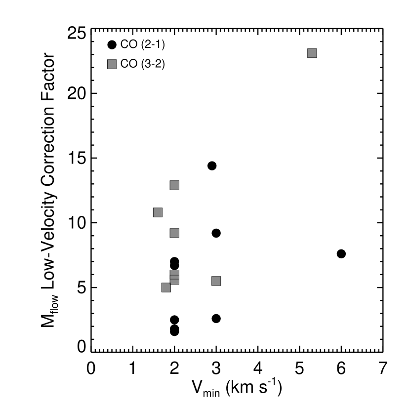
Figure 11.— Total low-velocity correction factor for $M_{\rm flow}$ plotted vs. $v_{\rm min}$, the lower bound of the velocity range used to calculate the outflow properties. Black circles show the corrections for outflows mapped in ¹²CO (2–1), and gray squares show the corrections for outflows mapped in ¹²CO (3–2).

Columns seven through 11 of Table 7 list the resulting factors by which $M_{\rm flow}$, $P_{\rm flow}$, $E_{\rm flow}$, $L_{\rm flow}$, and $F_{\rm flow}$ increase compared to the opacity-corrected values integrated between $v_{\rm min}$ and $v_{\rm max}$. We do not list corrections when we can’t obtain satisfactory Gaussian fits to the ambient cloud emission (usually due to offpositions contaminated with emission near the cloud rest velocities) or when $v_{\rm min}=1$ km s^-1 and corrections are thus uncessary. The middle row of Figure 5 shows the distribution of correction factors separately for the outflows mapped in each transition and combined. For the combined sample, we find that the outflow mass is increased by factors ranging from 1.6 to 23.1, with a mean (median) of 7.7 (6.7). The corrections are smaller for the other properties (increases by mean factors of 4.8, 3.3, 3.4, and 5.1 for $P_{\rm flow}$, $E_{\rm flow}$, $L_{\rm flow}$, and $F_{\rm flow}$, respectively), as expected since they depend on velocity to the first ($P_{\rm flow}$, $F_{\rm flow}$) or second ($E_{\rm flow}$, $L_{\rm flow}$) power and are less affected by emission at low velocities. As demonstrated by Figure 11, there is no significant correlation between $v_{\rm min}$ and the size of the correction factors. However, several outflows with $v_{\rm min}>2.0$ km s^-1 are not plotted here since satisfactory Gaussian fits could not be obtained due to contaminated off-positions, potentially masking the expected trend of increasing correction factors with increasing $v_{\rm min}$.

While our results indicate that significant fractions of the total mass, momentum, and energy of outflows can be missed by only integrating above a minimum velocity, we stress that the exact factors found here are highly uncertain and depend on the ambient cloud mass spectrum being well-fit by a simple Gaussian. Nevertheless, our results are generally consistent with those of Offner et al. (2011), who applied the same procedure to their synthetic observations of simulated outflows and concluded that only integrating beyond 2 km s^-1 from rest could lead to underestimates in $M_{\rm flow}$ by factors of 5–10. However, their results were based on only comparing to the total ejected mass in the simulations, since they were unable to track the total entrained mass; the true underestimates may be even larger.

Finally, we note that both our results and those of Offner et al. (2011) are unable to correct for the mass at the lowest velocities (in our case, within $\pm 1$ km s^-1 from rest). Using a very different method based on comparing the spectra at each position in an outflow to a reference spectrum constructed from nearby, off-outflow positions, both Maury et al. (2009) and van der Marel et al. (2013) did correct for missing mass all the way down to the ambient cloud velocity. Maury et al. (2009) found that $M_{\rm flow}$ increases by factors ranging from 3.9 to 42.1, with a mean (median) of 15.1 (12.7). These corrections, which they stress should be treated as upper limits, are approximately a factor of two larger than our mean and median corrections. On the other hand, van der Marel et al. (2013) found that $F_{\rm flow}$ only increases by factors that are generally less than $\sim 2$ (they do not discuss corrections for $M_{\rm flow}$), lower than found either by us or by Maury et al. (2009) and Offner et al. (2011). At present we do not have a satisfactory explanation for this discrepancy and note this remains an open question subject to further study. While the exact corrections remain quite uncertain and dependent on the exact procedure used to develop them, our findings coupled with those of most other recent studies indicate that adopting minimum velocities for integrating outflow properties can lead to significant underestimates.

4.4. Sensitivity

With the very high spectral resolution of many of our maps, we can evaluate whether high-velocity outflow emission below the sensitivities of our observations affects our results. While such emission is unlikely to significantly affect the total $M_{\rm flow}$ due to the steeply declining nature of outflow mass spectra (see §4.3 and Figure 10), it may affect the total $P_{\rm flow}$ and $E_{\rm flow}$, which are more heavily weighted toward the highest-velocity emission. To evaluate this effect, we smoothed each map with a native $\delta v\leq 0.2$ km s^-1 down to $\delta v=0.5$ km s^-1 and recalculated the outflow properties, with 0.5 km s^-1 chosen as the best compromise between increasing the sensitivity in high-velocity channels and retaining sufficient velocity resolution to fully resolve the kinematic structure of the outflows. Since $\delta v=0.5$ km s^-1 is too low of a velocity resolution to reliably fit to the ambient cloud emission at $\pm 1$ km s^-1, we only integrated for velocities above $v_{\rm min}$ and compared to the values obtained from the higher resolution maps over the same velocity range.

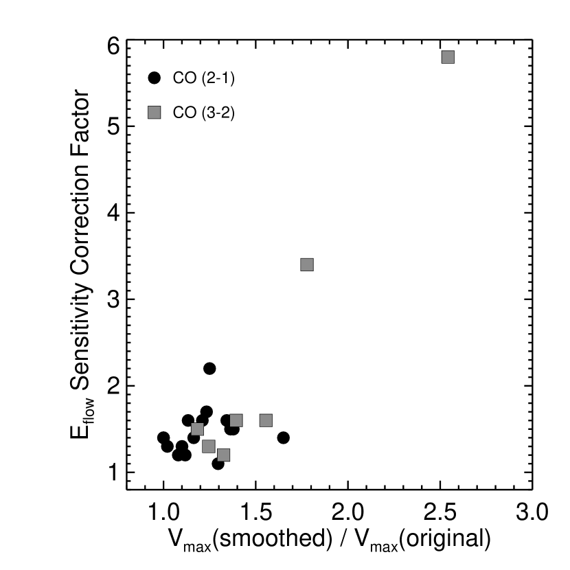
Figure 12.— Total sensitivity correction factor for $E_{\rm flow}$ plotted versus the ratio of maximum velocities of detected emission in the maps smoothed to 0.5 km s^-1 resolution to those in the original maps. Black circles show the corrections for outflows mapped in ¹²CO (2–1), and gray squares show the corrections for outflows mapped in ¹²CO (3–2).

Columns 12 through 16 of Table 7 list the resulting factors by which $M_{\rm flow}$, $P_{\rm flow}$, $E_{\rm flow}$, $L_{\rm flow}$, and $F_{\rm flow}$ increase when these sensitivity corrections are made. These factors are multiplicative with those listed in other columns and discussed in previous Sections. The bottom row of Figure 5 shows the distribution of correction factors separately for the outflows mapped in each transition and combined. For the combined sample, we find that the outflow mass is only increased by factors ranging from 1.0 to 2.4, with a mean (median) increase of 1.4 (1.3). However, as expected, the corrections are larger for $P_{\rm flow}$ and $E_{\rm flow}$ (increases by mean factors of 1.5 and 1.7, respectively, and maximum increases by factors of 2.8 and 5.8, respectively), since both are weighted to higher-velocity emission. The corrections for $L_{\rm flow}$ and $F_{\rm flow}$ are even larger (increases by mean factors of 2.6 and 2.1), since their numerators increase while their denominators ($t_{\rm dyn}$) simultaneously decrease due to increases in $v_{\rm max}$. Figure 12 shows that larger correction factors are derived for larger increases in the maximum velocity at which outflow emission is detected between the original and smoothed maps.

These results emphasize that significant underestimates in the kinematic properties of outflows are possible when lacking sufficient sensitivity to detect the highest-velocity emisison. Furthermore, they disagree with those of van der Marel et al. (2013), who argued that the sensitivity and spectral binning of the observations do not significantly affect the calculated properties. We note that qualitatively similar results to our own were found by Arce et al. (2013), who used ALMA observations of HH 46/47 to detect outflow emission at higher velocities than previously detected in single-dish observations with lower sensitivity, and calculated correction factors of about 1, 4, and 11 for $M_{\rm flow}$, $P_{\rm flow}$, and $E_{\rm flow}$, respectively (Arce 2013, priv. comm.). While it is impossible to quantify the magnitude of this effect for all cases, since it depends on the sensitivity of the observations, we note that the sensitivity of our observations are generally comparable to those of other large, single-dish surveys of molecular outflows (e.g., Bontemps et al., 1996; Hatchell et al., 2007a; Hatchell & Dunham, 2009; Maury et al., 2009; Curtis et al., 2010b). Future studies should carefully evaluate the magnitude of this effect in their data.

Finally, we note that the extremely high velocity (EHV) components of molecular outflows that are common in outflows driven by massive protostars (e.g., Choi et al., 1993), typically at velocities in excess of 50 km s^-1 from rest, are also sometimes found in outflows driven by low-mass protostars (e.g., Tafalla et al., 2004). As they are often both compact and weak, the beam dilution from our single dish observations with low spatial resolution render them undetectable in our data (as confirmed by nondetections of EHV components for IRAS 03271$+$3013, IRAS 03282$+$3035, HH211, or IRAS 04166$+$2706, all of which are known to have such components; Bachiller et al., 1991; Gueth & Guilloteau, 1999; Tafalla et al., 2004). While such components increase the total $M_{\rm flow}$ by negligible amounts, they can contain up to $2-4$ times as much momentum and energy as the lower-velocity outflow components (e.g., Tafalla et al., 2004). Sensitive interferometer observations with high spatial resolution are needed to search for EHV components missed by our maps.

4.5. Other Possible Corrections

Table 8Inclination Corrections for Motions Along Jet Axis

	Inclination	Corrections
Quantity	Dependence	$\langle i\rangle=57.3$∘	$i=15$∘	$i=85$∘
$R_{\rm lobe}$	$1/{\rm sin}\,i$	1.2	11.5	1.0
$\tau_{\rm d}$	${\rm cos}\,i/{\rm sin}\,i$	0.6	11.4	0.09
$M_{\rm flow}$	$\cdots$	$\cdots$	$\cdots$	$\cdots$
$P_{\rm flow}$	$1/{\rm cos}\,i$	1.9	1.0	11.5
$E_{\rm flow}$	$1/{\rm cos}^{2}\,i$	3.4	1.10	131.6
$L_{\rm flow}$	${\rm sin}\,i/{\rm cos}^{3}\,i$	5.3	0.09	1504.7
$F_{\rm flow}$	${\rm sin}\,i/{\rm cos}^{2}\,i$	2.9	0.09	131.1

Since we can only measure the radial component of the total velocity of outflowing gas and the projection of the outflow lobe size on the plane of the sky, corrections for source inclination, $i$, are necessary, where $i$ is the angle between the rotation/outflow axis and the observer ($i=0$^∘ corresponds to a pole-on system, and $i=90$^∘ corresponds to an edge-on system). The second column of Table 8 lists the inclination dependence for each outflow property for outflows where all of the motion is along the jet axis. Since we are unable to measure opening angles of the outflows mapped here, we are also unable to derive reliable inclination constraints (see §3.1). Thus, Table 8 lists the correction factors for a mean inclination angle $\langle i\rangle=57.3$^∘ (assuming all orientations are equally favorable) and for nearly pole-on (5^∘) and nearly edge-on (85^∘) inclinations. For the mean inclination angle, $P_{\rm flow}$, $E_{\rm flow}$, $L_{\rm flow}$, and $F_{\rm flow}$ increase, on average, by factors of 1.9, 3.4, 5.3, and 2.9, respectively. The correction factors for $P_{\rm flow}$ and $E_{\rm flow}$ are always greater than or equal to 1.0 for all possible inclinations. For $L_{\rm flow}$ and $F_{\rm flow}$, they are greater than or equal to 1.0 for $i\geq 38.2$^∘ and $i\geq 24.4$^∘, respectively. Since the probabilities of viewing sources at lower inclinations are only 21% and 18%, respectively, these corrections are greater than or equal to 1.0 the majority of the time.

The corrections listed in Table 8 are only valid for outflows where all of the motion is along the jet axis. Using simulations, Downes & Cabrit (2007) also investigated inclination corrections taking into account transverse motions due to sideways expansion. They showed that the correction factor of $1/{\rm cos}\,i$ for $P_{\rm flow}$ always overestimates the true momentum. They found that, by coincidence, the uncorrected $P_{\rm flow}$ always agrees with the true value to within a factor of two since underestimates of the momentum along the jet axis are canceled by overestimates due to the erroneous inclusion of transverse momentum. Similarly, they also showed that the correction factor of $1/{\rm cos}^{2}\,i$ for $E_{\rm flow}$ also overestimates the true energy. Unlike for momentum, however, the uncorrected values of $E_{\rm flow}$ do still underestimate the total energy for many inclinations. However, we note that these results only apply for outflows from Class 0 protostars that are driven solely by jets and which have not yet broken out of their parent clouds, so they may not apply to all of the outflows studied here.

Table 9Corrected Outflow Dynamical Properties

	$v_{\rm min}$	$v_{\rm max}$	$M_{\rm flow}$	$P_{\rm flow}$	$E_{\rm flow}$	$\tau_{\rm d}$	$L_{\rm flow}$	$F_{\rm flow}$
Source	(km s-1)	(km s-1)	(M⊙)	(M⊙ km s-1)	(ergs)	(yr)	(L⊙)	(M⊙ km s-1 yr-1)
12CO (2–1)
IRAS 03235$+$3004	2.0	5.1	$\geq$5.0${}\times 10^{-1}$	$\geq$7.8${}\times 10^{-1}$	$\geq$1.3${}\times 10^{43}$	4.2${}\times 10^{4}$	2.5${}\times 10^{-3}$	1.9${}\times 10^{-5}$
IRAS 03282$+$3035	6.0	25.9	4.3${}\times 10^{-1}$	2.1${}\times 10^{0}$	1.4${}\times 10^{44}$	1.1${}\times 10^{4}$	1.0${}\times 10^{-1}$	1.9${}\times 10^{-4}$
HH211	2.9	9.9	1.1${}\times 10^{-1}$	2.3${}\times 10^{-1}$	5.5${}\times 10^{42}$	7.3${}\times 10^{3}$	6.6${}\times 10^{-3}$	3.4${}\times 10^{-5}$
L1709-SMM1	1.5	2.3	$\geq$8.6${}\times 10^{-3}$	$\geq$1.5${}\times 10^{-2}$	$\geq$2.6${}\times 10^{41}$	3.3${}\times 10^{4}$	$\geq$6.8${}\times 10^{-5}$	$\geq$4.7${}\times 10^{-7}$
L1709-SMM5	2.0	5.7	$\geq$5.7${}\times 10^{-2}$	$\geq$1.3${}\times 10^{-1}$	$\geq$3.2${}\times 10^{42}$	$\cdots$	$\cdots$	$\cdots$
CB68	1.0	2.0	1.6${}\times 10^{-2}$	1.9${}\times 10^{-2}$	2.1${}\times 10^{41}$	5.4${}\times 10^{4}$	3.2${}\times 10^{-5}$	3.4${}\times 10^{-7}$
Aqu-MM2	3.0	9.8	$\geq$2.9${}\times 10^{-2}$	$\geq$1.4${}\times 10^{-1}$	$\geq$6.7${}\times 10^{42}$	1.1${}\times 10^{4}$	$\geq$5.3${}\times 10^{-3}$	$\geq$1.2${}\times 10^{-5}$
Aqu-MM3	3.0	9.2	1.6${}\times 10^{-1}$	5.1${}\times 10^{-1}$	1.5${}\times 10^{43}$	1.5${}\times 10^{4}$	8.7${}\times 10^{-3}$	3.0${}\times 10^{-5}$
Aqu-MM5	3.0	9.2	1.8${}\times 10^{-1}$	3.9${}\times 10^{-1}$	9.1${}\times 10^{42}$	2.5${}\times 10^{4}$	3.0${}\times 10^{-3}$	1.5${}\times 10^{-5}$
SerpS-MM13	5.5	14.3	$\geq$8.8${}\times 10^{-2}$	$\geq$6.4${}\times 10^{-1}$	$\geq$5.2${}\times 10^{43}$	2.6${}\times 10^{4}$	$\geq$1.7${}\times 10^{-2}$	$\geq$2.3${}\times 10^{-5}$
CrA-IRAS32	2.0	4.6	$\geq$1.1${}\times 10^{-2}$	$\geq$2.7${}\times 10^{-2}$	$\geq$6.7${}\times 10^{41}$	2.1${}\times 10^{4}$	$\geq$2.6${}\times 10^{-4}$	$\geq$1.2${}\times 10^{-6}$
L673-7	3.0	8.1	$\geq$5.5${}\times 10^{-2}$	$\geq$2.1${}\times 10^{-1}$	$\geq$7.7${}\times 10^{42}$	2.6${}\times 10^{4}$	$\geq$2.3${}\times 10^{-3}$	$\geq$7.4${}\times 10^{-6}$
B335	1.0	5.5	9.9${}\times 10^{-2}$	1.7${}\times 10^{-1}$	3.3${}\times 10^{42}$	4.2${}\times 10^{4}$	6.4${}\times 10^{-4}$	4.0${}\times 10^{-6}$
L1152	2.0	4.7	$\geq$7.5${}\times 10^{-1}$	$\geq$1.2${}\times 10^{0}$	$\geq$1.9${}\times 10^{43}$	7.0${}\times 10^{4}$	2.4${}\times 10^{-3}$	1.7${}\times 10^{-5}$
L1157	2.0	25.6	6.1${}\times 10^{-1}$	3.1${}\times 10^{0}$	1.5${}\times 10^{44}$	1.0${}\times 10^{4}$	1.1${}\times 10^{-1}$	1.8${}\times 10^{-4}$
L1165	2.0	3.7	1.6${}\times 10^{-1}$	3.1${}\times 10^{-1}$	6.2${}\times 10^{42}$	7.7${}\times 10^{4}$	6.7${}\times 10^{-4}$	4.2${}\times 10^{-6}$
L1251A-IRS3	2.3	5.3	$\geq$1.1${}\times 10^{-1}$	$\geq$3.4${}\times 10^{-1}$	$\geq$1.1${}\times 10^{43}$	6.8${}\times 10^{4}$	$\geq$1.3${}\times 10^{-3}$	$\geq$5.1${}\times 10^{-6}$
12CO (3–2)
IRAS 03235$+$3004	2.6	5.7	$\geq$1.1${}\times 10^{-3}$	$\geq$3.5${}\times 10^{-3}$	$\geq$1.3${}\times 10^{41}$	1.1${}\times 10^{4}$	$\geq$9.6${}\times 10^{-5}$	$\geq$3.1${}\times 10^{-7}$
IRAS 03271$+$3013	1.8	6.1	$\geq$1.8${}\times 10^{-2}$	$\geq$3.6${}\times 10^{-2}$	$\geq$8.2${}\times 10^{41}$	1.1${}\times 10^{4}$	6.4${}\times 10^{-4}$	3.2${}\times 10^{-6}$
IRAS 03282$+$3035	3.0	13.8	$\geq$6.6${}\times 10^{-2}$	$\geq$1.9${}\times 10^{-1}$	$\geq$7.0${}\times 10^{42}$	4.8${}\times 10^{3}$	1.1${}\times 10^{-2}$	4.0${}\times 10^{-5}$
HH211	2.0	2.7	5.6${}\times 10^{-2}$	1.2${}\times 10^{-1}$	2.6${}\times 10^{42}$	2.5${}\times 10^{4}$	1.5${}\times 10^{-3}$	8.4d-6${}\times 10^{-3}$
IRAS 04166$+$2706	2.0	2.5	$\geq$6.5${}\times 10^{-4}$	$\geq$1.5${}\times 10^{-3}$	$\geq$3.4${}\times 10^{40}$	2.0${}\times 10^{4}$	$\geq$9.6${}\times 10^{-6}$	$\geq$5.3${}\times 10^{-8}$
IRAM 04191$+$1522	2.0	7.7	4.2${}\times 10^{-2}$	1.4${}\times 10^{-1}$	2.0${}\times 10^{42}$	1.4${}\times 10^{4}$	1.2${}\times 10^{-3}$	6.4${}\times 10^{-6}$
HH25	4.0	10.5	$\geq$1.8${}\times 10^{-2}$	$\geq$8.5${}\times 10^{-2}$	$\geq$4.5${}\times 10^{42}$	9.9${}\times 10^{3}$	$\geq$3.7${}\times 10^{-3}$	$\geq$8.5${}\times 10^{-6}$
HH26	4.0	24.5	$\geq$2.7${}\times 10^{-1}$	$\geq$2.0${}\times 10^{0}$	$\geq$1.8${}\times 10^{44}$	1.2${}\times 10^{4}$	$\geq$1.3${}\times 10^{-1}$	$\geq$1.6${}\times 10^{-4}$
BHR86	2.0	5.6	1.4${}\times 10^{-1}$	2.4${}\times 10^{-1}$	5.1${}\times 10^{42}$	3.4${}\times 10^{4}$	1.2${}\times 10^{-3}$	7.0${}\times 10^{-6}$
IRAS 15398$-$3359	2.0	5.8	$\geq$3.7${}\times 10^{-4}$	$\geq$1.2${}\times 10^{-3}$	$\geq$3.7${}\times 10^{40}$	2.5${}\times 10^{3}$	$\geq$1.2${}\times 10^{-4}$	$\geq$4.5${}\times 10^{-7}$
Lupus 3 MMS	2.0	4.0	3.1${}\times 10^{-2}$	4.8${}\times 10^{-2}$	8.1${}\times 10^{41}$	2.5${}\times 10^{4}$	2.7${}\times 10^{-4}$	1.9${}\times 10^{-6}$
L483	5.3	8.9	2.8${}\times 10^{-2}$	1.1${}\times 10^{-1}$	3.7${}\times 10^{42}$	1.2${}\times 10^{4}$	2.6${}\times 10^{-3}$	9.0${}\times 10^{-6}$
L673-7	2.0	4.6	$\geq$1.0${}\times 10^{-2}$	$\geq$2.6${}\times 10^{-2}$	$\geq$7.0${}\times 10^{41}$	4.6${}\times 10^{4}$	$\geq$1.2${}\times 10^{-4}$	$\geq$5.5${}\times 10^{-7}$
L1157	1.4	21.1	$\geq$1.5${}\times 10^{-1}$	$\geq$5.5${}\times 10^{-1}$	$\geq$3.8${}\times 10^{43}$	1.2${}\times 10^{4}$	$\geq$2.6${}\times 10^{-2}$	$\geq$4.7${}\times 10^{-5}$
L1228	2.0	12.0	$\geq$8.7${}\times 10^{-2}$	$\geq$3.2${}\times 10^{-1}$	$\geq$1.4${}\times 10^{43}$	2.4${}\times 10^{4}$	$\geq$4.8${}\times 10^{-3}$	$\geq$1.3${}\times 10^{-5}$
L1014	1.3	3.0	$\geq$3.1${}\times 10^{-4}$	$\geq$5.6${}\times 10^{-4}$	$\geq$9.9${}\times 10^{39}$	2.4${}\times 10^{4}$	$\geq$3.5${}\times 10^{-6}$	$\geq$2.3${}\times 10^{-8}$
L1165	1.6	4.0	5.7${}\times 10^{-2}$	8.3${}\times 10^{-2}$	1.4${}\times 10^{42}$	4.5${}\times 10^{4}$	2.6${}\times 10^{-4}$	1.9${}\times 10^{-6}$

Ultimately, given our inability to determine inclinations for most sources and the uncertainties over the correct inclination factors to apply, we do not correct our outflow properties for inclination. As a result, even our corrected outflow properties are strictly lower limits, since inclination corrections will generally only increase these properties based on the above arguments, especially for nearly edge-on systems.

Additional correction factors must be applied if some of the outflowing gas is atomic. Downes & Cabrit (2007) investigated this possibility with numerical simulations and found that the fraction of gas dissociated in strong shocks becomes progressively larger for gas outflowing at larger velocities. They used these results to show that properties measured only from observations of molecular gas underestimated the true values by factors of 1.6 for $M_{\rm flow}$, $2-4$ for $P_{\rm flow}$ and $F_{\rm flow}$, and $3-7$ for $E_{\rm flow}$ and $L_{\rm flow}$. We are unable to evaluate the effects of dissociation with our data.

Finally, the method of calculation itself can lead to significant differences in calculated outflow properties. These effects were recently explored in detail by van der Marel et al. (2013), who found a factor of six spread in $F_{\rm flow}$ depending on the exact method of calculation. Our method of calculating $F_{\rm flow}$ is identical to their method M7, which they conclude is the least affected by uncertain observational parameters.

5. Discussion

5.1. Correction Factors

In the previous sections we have explored in detail the corrections to outflow properties that must be applied to correct for optical depth of the ¹²CO transitions, outflowing gas at low velocities that overlap with the velocities of the ambient cloud gas, and outflowing gas below the sensitivities of the individual maps. These corrections are tabulated in Table 7, and are multiplicative. Multiplying all three together, we find that the mean total correction factors are 13.1, 9.5, 7.6, 10.2, and 12.4 for $M_{\rm flow}$, $P_{\rm flow}$, $E_{\rm flow}$, $L_{\rm flow}$, and $F_{\rm flow}$, respectively. In the most extreme cases, they extend up to factors of 59.6, 54.9, 52.4, 88.6, and 89.8 for the five quantities, and possibly even higher since we are unable to determine corrections for low-velocity outflow emission for 15 of the 34 outflows in our sample. Outflow studies that fail to correct for one or more of these effects risk underestimating the masses and dynamical properties of the outflows by up to two orders of magnitude, and possibly even more in the most extreme cases.

Table 9 presents the same properties for each outflow as Table 6, except now with the corrections listed in Table 7 applied. Even after applying these corrections, it is very likely that our final values of outflow masses and dynamical properties reported in Table 9 are still underestimates. The corrections for both opacity and outflowing gas at low velocities are conservative, as discussed in Sections 4.1 and 4.3, respectively, and the sensitivity corrections are limited by the fact that we can only smooth the original maps so far in velocity while still preserving the basic kinematic structure of the outflows. Furthermore, excitation temperatures greater than 50 K, such as those found by van Kempen et al. (2009c, d), non-uniform excitation temperatures with warmer gas at higher velocities, inclination effects, and dissociation of molecular gas in strong shocks will all work to further increase the properties of each outflow, as discussed in detail in previous Sections. We thus caution that molecular outflows are almost certainly significantly more massive and energetic than found by most analyses of low-J rotational transitions of ¹²CO, including our own results presented in this study. Exactly how much more massive and energetic is impossible to quantify in a general sense because it depends on the assumptions and methods of each particular study, as well as quantities (inclination, fraction of material that is dissociated, etc.) that are not always possible to measure. Nevertheless, these results must be kept in mind when evaluating the masses and energtics of outflows and their impact on their environments.

5.2. Comparing the Two Transitions of ¹²CO

Six of the outflows in this study are mapped in both ¹²CO (2–1) and ¹²CO (3–2): IRAS 03235$+$3004, IRAS 03282$+$3035, HH211, L673-7, L1157, and L1165. Inspection of Tables 6 and 9 shows that the values of $M_{\rm flow}$ and all dynamical properties ($P_{\rm flow}$, $E_{\rm flow}$, $L_{\rm flow}$, and $F_{\rm flow}$) are systematically lower when calculated from the ¹²CO (3–2) transition. To further investigate this trend, we first remove any possible effects from different spatial and spectral resolutions and sensitivities by convolving the ¹²CO (3–2) maps (which always have higher spatial resolution) down to the resolution of the ¹²CO (2–1) maps and then aligning both onto a common spatial and spectral pixel grid, masking out spatial pixels that are not covered by both transitions to ensure complete overlap. We then calculate the rms noise in each map and clip out all emission below three times the larger of the noises in the two transitions, which effectively degrades the sensitivity of the deeper map to match that of the other transition. We then recalculate opacity-corrected outflow properties from each transition, integrating over a common velocity interval for each transition with $v_{\rm min}$ chosen to be large enough to eliminate all possible confusion with ambient cloud emission and $v_{\rm max}$ chosen to extend only to the smaller of the two $v_{\rm max}$ for each transition. In this manner we ensure that we are only comparing emission from the outflows, over velocities where both outflows are detected.

Table 10¹²CO (2–1) versus ¹²CO (3–2) as an Outflow Tracer

Source	$M_{\rm flow}$21/$M_{\rm flow}$32	$F_{\rm flow}$21/$F_{\rm flow}$32
IRAS 03235$+$3004	10.2	10.5
IRAS 03282$+$3035	4.3	5.0
HH211	1.6	1.4
L673-7	11.4	7.0
L1157	2.1	2.0
L1165	20.0	13.5

Figure 13.— The factor by which the ratio of $M_{\rm flow}$ calculated from ¹²CO (3–2) to that calculated from ¹²CO (2–1) will change for different values of $T_{\rm ex}$, compared to the ratio calculated assuming $T_{\rm ex}=50$ K. See Appendix C for details on the calculation.

The results of this process are listed in Table 10 for $M_{\rm flow}$ and $F_{\rm flow}$; similar results are obtained for the other dynamical properties. Both quantities are systematically higher when calculated from the ¹²CO (2–1) maps than the ¹²CO (3–2) maps. The mean increase in $M_{\rm flow}$ for these six outflows is 8.3, with individual values ranging from 1.6 to 20. As long as the gas has $T_{\rm ex}\gtrsim 20$ K the intensity will be as bright or brighter in the (3–2) transition than the (2–1) transition, so missing (3–2) emission below the sensitivities of the maps is not a likely explanation since we only integrate emission above a common sensitivity. Thus any emission bright enough to detect in ¹²CO (2–1) should also be bright enough to detect in ¹²CO (3–2), unless $T_{\rm ex}$ is significantly below 20 K (which we consider unlikely; see §4.2). Another possible explanation for this discrepancy is that our assumed $T_{\rm ex}$ of 50 K is wrong, since the mass ratio between the two transitions will change for different temperatures. However, as shown by Figure 13, increasing the ratio of $M_{\rm flow}$ by a factor of 8.3 requires decreasing the assumed $T_{\rm ex}$ to below 10 K, and increasing this ratio by a factor of 20 requires decreasing the assumed $T_{\rm ex}$ to $\sim$ 5 K (see Appendix C for details on the calculation). Such low temperatures are required because it is only at these very low temperatures that the relative population of the $J=3$ state compared to the $J=2$ state decreases substantially, but $T_{\rm ex}<10$ K is highly unlikely for gas in molecular outflows (see §4.2). A third possible explanation is that higher-J transitions of ¹²CO are dominated by emission of gas at higher temperatures, as suggested by recent Herschel detections of warm ¹²CO (up to $\sim 1000$ K; e.g., Green et al., 2013; Yıldız et al., 2013; Santangelo et al., 2013) associated with low-mass protostars. However, as seen by Figure 7, even increasing the assumed $T_{\rm ex}$ to 200 K for ¹²CO (3–2) fails to resolve the discrepancy for most sources, and such extreme temperature differences between the gas dominating the emission in two successive rotational levels with energies that are separated by less than 20 K are unlikely. Non-LTE radiative transfer modeling would be required to fully explore these effects, but such work is beyond the scope of this paper.

An additional potential explanation recently put forth by Ginsburg et al. (2011) is that the ¹²CO (3–2) line is subthermally excited and thus a poor tracer of total mass. The critical density of the (3–2) transition is about 20 times higher than that of the (1–0) transition. Ginsburg et al. (2011) used RADEX, a one-dimensional, non-LTE radiative transfer code (van der Tak et al., 2007) to show that the total outflow mass calculated from ¹²CO (3–2) can be underestimated by up to 1–2 orders of magnitude for gas densities between 10² and 10⁴ cm^-3. Since the (2–1) transition may also be subthermally excited in some cases (its critical density is about six times higher than that for the ground-state transition) the difference between outflow masses calculated from the (3–2) and (2–1) transitions are likely equal to or less than the ¹²CO (3–2) underestimates calculated by Ginsburg et al. (2011), consistent with our results listed in Table 10. Since we have rejected sensitivity and the assumed $T_{\rm ex}$ as explanations for the discrepancy in outflow properties calculated from the (3–2) and (2–1) transitions, our results are consistent with the claim by Ginsburg et al. (2011) that the ¹²CO (3–2) line is subthermally excited in molecular outflows and thus a poor tracer of total outflow mass.

While our results are based on only six outflows and require confirmation with a larger sample, they have important implications. Many recent studies focusing on topics including the evolution of outflows, the link between outflows and protostellar accretion, and the impact of outflow feedback on cluster-scale star formation have primarily used observations of ¹²CO (3–2), both because it can be mapped with the same telescope at higher angular resolution than lower-J transitions and because it is easier to separate warm outflowing gas from cold ambient gas in higher-J transitions (e.g., Hatchell et al., 2007a; Hatchell & Dunham, 2009; Curtis et al., 2010b; Nakamura et al., 2011). If Ginsburg et al. (2011) are correct and the ¹²CO (3–2) line is subthermally excited in outflows, as indeed suggested by our results, all of these studies have likely underestimated the total mass, momentum, and energy of the outflows in their samples, and conclusions based on these quantities will need to be revisited. Confirming our results with a larger sample of outflows, and extending this comparison to the ¹²CO (1–0) transition, are noted as critical directions for future work to pursue.

6. Summary

In this paper we have presented the first results of a survey of 28 molecular outflows driven by low-mass protostars, all of which are sufficiently isolated spatially and/or kinematically to fully separate into individual outflows. Using a combination of new and archival data from several single-dish telescopes, 17 outflows were mapped in ¹²CO (2–1) and 17 are mapped in ¹²CO (3–2), with 6 mapped in both transitions. We summarize our main results as follows:

1. For each outflow, we calculate and tabulate the mass ($M_{\rm flow}$), momentum ($P_{\rm flow}$), kinetic energy ($E_{\rm flow}$), mechanical luminosity ($L_{\rm flow}$), and force ($F_{\rm flow}$) assuming optically thin emission in LTE at an excitation temperature, $T_{\rm ex}$, of 50 K. We also tabulate the size of each outflow and its position angle on the sky.

2. For outflows mapped in both transitions of ¹²CO, line ratios suggest excitation temperatures ranging from 10 – 20 K. While there is very weak evidence for higher temperatures (up to 50 K) at the highest redshifted velocities, in general there is no clear trend with velocity. However, with only these two low-J rotational transitions of ¹²CO, we are insensitive to the presence of warmer gas. We thus adopt 50 K as the most likely value based on results from other authors that find such temperatures.

3. All of the calculated outflow properties are significantly underestimated when calculated from the original data under the assumption of optically thin emission in LTE, with velocity ranges chosen to avoid contamination by ambient cloud emission. Taken together, the effects of opacity, outflow emission at low velocities confused with ambient cloud emission, and emission below the sensitivities of the observations increase outflow masses and dynamical properties by an order of magnitude, on average, and factors of 50–90 in the most extreme cases.

4. Different (and non-uniform) excitation temperatures, inclination effects, and dissociation of molecular gas will all work to further increase the masses and dynamical properties of outflows. Molecular outflows are thus almost certainly more massive and energetic than commonly reported.

5. For outflows mapped in both transitions, the masses and dynamical properties are lower, on average, by about an order of magnitude when calculated from the ¹²CO (3–2) maps compared to the ¹²CO (2–1) maps, even after accounting for different opacities, map sensitivities, and possible excitation temperature variations. Ginsburg et al. (2011) argued that the ¹²CO (3–2) line is subthermally excited in outflows, and our results support this finding.

We have provided a systematic analysis of the uncertainties in and necessary corrections to typical calculations of outflow masses and dynamical properties. Studies that neglect one or more of these effects will underestimate the properties of molecular outflows; not only does this indicate that outflows are more massive and energetic than commonly found, but it also suggests that outflows may have larger impacts on the turbulence and energetics of their environments than is often calculated based on studies of outflows in clustered regions (e.g., Arce et al., 2010; Nakamura et al., 2011; Plunkett et al., 2013). In a forthcoming paper we will explore the effects of these corrections on our understanding of the evolution of outflows and the link between protostellar accretion and outflow activity. Several avenues of future work remain necessary. First, larger, more sensitive maps of ¹³CO are necessary in order to derive separate velocity-dependent opacity corrections for each outflow, and perhaps even for each position in each outflow, rather than the corrections averaged over many outflows that we derive here. Additionally, higher-J transitions of ¹²CO are needed to fully evaluate the excitation temperatures of the outflows and identify any variations with position and/or velocity. Finally, a larger sample of outflows must be mapped in multiple transitions of ¹²CO in order to confirm our findings that the ¹²CO (3–2) line underestimates outflow masses and dynamical properties due to subthermal excitation, as recently argued by Ginsburg et al. (2011).

Appendix A A.  Summary of Individual Sources

In this section we provide a brief description of each source surveyed in this paper.

A.1. IRAS 03235$+$3004

IRAS 03235$+$3004 (hereafter IRAS03235) is a protostar embedded in the southwestern portion of the Perseus Molecular Cloud, on the western edge of L1455. For this and all other sources in Perseus we adopt a distance of 250 pc (Enoch et al., 2006, and references therein), consistent with the VLBI maser parallax distance of 235 $\pm$ 18 pc for NGC 1333 determined by Hirota et al. (2008). IRAS03235 is embedded within a $0.5-2.5$ M_⊙ core (Enoch et al., 2006, 2009; Hatchell et al., 2005, 2007b) that exhibits spectroscopic signatures of infall (Gregersen et al., 2000) and is located at a rest velocity of 5.1 km s^-1 (Mardones et al., 1997; Kirk et al., 2007). It is detected at 2 $\mu$m (Ladd et al., 1993) and is classified as a borderline Class 0/I object based on the full observed SED, including Spitzer Space Telescope (Werner et al., 2004) $3.6-70$ $\mu$m detections (Jørgensen et al., 2006; Rebull et al., 2007), with individual estimates of $T_{bol}$ ranging between 68 and 136 K (Mardones et al., 1997; Hatchell et al., 2007b; Enoch et al., 2009; Evans et al., 2009). IRAS03235 drives a bipolar molecular outflow detected by Hatchell & Dunham (2009).

A.2. IRAS 03271$+$3013

IRAS 03271$+$3013 (hereafter IRAS03271) is an embedded protostar located south of NGC1333 in the Perseus Molecular Cloud at a distance of 250 pc (see above). The surrounding core has a mass of $0.5-5$ M_⊙ (Bachiller et al., 1991; Ladd et al., 1994; Hatchell et al., 2005, 2007b; Enoch et al., 2006, 2009), is located at a rest velocity of 5.9 km s^-1 (Bachiller et al., 1991; Ladd et al., 1994; Kirk et al., 2007; Rosolowsky et al., 2008; Hatchell & Dunham, 2009; Emprechtinger et al., 2009), and shows no evidence for strong deuteration or infall (Emprechtinger et al., 2009). IRAS03271 is detected in the near-infrared at 2 $\mu$m (Ladd et al., 1993) and in the mid-infrared at $3.6-70$ $\mu$m with Spitzer (Jørgensen et al., 2006; Rebull et al., 2007) and is classified as a Class I protostar, with individual estimates of $T_{bol}$ ranging between 97 and 133 K (Hatchell et al., 2007b; Enoch et al., 2009; Evans et al., 2009). It drives a bipolar molecular outflow (Bachiller et al., 1991; Hatchell & Dunham, 2009) that extends to extremely high velocities (up to $\sim$40 km s^-1 from rest), it is associated with a faint 2 $\mu$m reflection nebula that extends along the outflow axis (Connelley et al., 2007), and it has been identified as the driving source of three Herbig-Haro objects (HH 368, 369, and 370; Wu et al., 2002).

A.3. IRAS 03282$+$3035

IRAS 03282$+$3035 (hereafter IRAS03282) is a well-studied, deeply embedded protostar located south of NGC1333 and west of B1 in the Perseus Molecular Cloud at a distance of 250 pc (see above). The surrounding core has a mass of $0.8-6.3$ M_⊙ (Bachiller et al., 1991; Barsony et al., 1998; Shirley et al., 2000; Motte & André, 2001; Hatchell et al., 2005, 2007b; Enoch et al., 2006, 2009), is located at a rest velocity of $7.1$ km s^-1 (Bachiller et al., 1991; Mardones et al., 1997; Gregersen et al., 2000; Hatchell et al., 2007a), shows strong deuteration (Roberts et al., 2002; Hatchell, 2003; Roberts & Millar, 2007; Emprechtinger et al., 2009) and no significant evidence of infall or fast rotation (Mardones et al., 1997; Gregersen et al., 2000; Chen et al., 2007). IRAS03282 is detected in the mid-infrared with Spitzer (Jørgensen et al., 2006; Rebull et al., 2007) and is classified as a Class 0 protostar, with individual estimates of $T_{bol}$ ranging between 23 and 60 K (Shirley et al., 2000; Hatchell et al., 2007b; Enoch et al., 2009; Evans et al., 2009).

IRAS03282 drives a strong bipolar molecular outflow first detected by (Bachiller et al., 1991). This outflow extends to extremely high velocities (greater than 50 km s^-1 relative to the core rest velocity) and features a highly collimated, jet-like structure at the highest velocities comprised of a series of high-velocity “bullets” or clumps (Bachiller et al., 1991). The velocities and spacings of these clumps suggest an episodicity in the mass ejection (and thus likely in the underlying mass accretion) on timescales of $\sim 10^{3}$ yr (Bachiller et al., 1991). This outflow is associated with near-infrared H₂ knots coincident with the high-velocity bullets, warm (T $>50-100$ K) NH₃, SiO emission, and enhanced CH₃OH abundance (Bally et al., 1993; Bachiller et al., 1993, 1994, 1995), and is consistent with models featuring time-dependent rather than steady-state jets (Bachiller et al., 1994).

A.4. HH211

HH211 was originally discovered as a jet detected in near-infrared continuum and narrow-band H₂ images (McCaughrean et al., 1994). It is located in the southwestern portion of IC348 in the Perseus Molecular Cloud at a distance of 250 pc (see above). The near-infrared jet consists of multiple knots, and it coincides with a molecular outflow that extends up to $\sim$50 km s^-1 from rest that is centered on a dense core detected in NH₃ and submillimeter and millimeter continuum observations (Bachiller et al., 1987; McCaughrean et al., 1994; Gueth & Guilloteau, 1999; Tanner & Arce, 2011). This core has a mass of $2.5-23$ M_⊙ (Motte & André, 2001; Kirk et al., 2006; Hatchell et al., 2005, 2007b; Enoch et al., 2006, 2009), is located at a rest velocity of 9.1 km s^-1 (Mardones et al., 1997; Gregersen et al., 2000; Hatchell et al., 2007a), and shows moderately strong deuteration (Roberts et al., 2002; Hatchell, 2003; Roberts & Millar, 2007; Emprechtinger et al., 2009) but no conclusive evidence for infall (Mardones et al., 1997; Gregersen et al., 2000). Embedded within this core is a Class 0 protostar detected in the far-infrared with ISO (Froebrich et al., 2003) and in the mid-infrared with Spitzer, but only at wavelengths longward of 24 $\mu$m (Rebull et al., 2007; Evans et al., 2009). Individual estimates of $T_{bol}$ for this protostar range from 21 to 31 K (Hatchell et al., 2007b; Enoch et al., 2009; Evans et al., 2009).

The molecular outflow driven by this source has been extensively studied over the past two decades. At low velocities the outflow traces the shells of cleared cavities whereas at high velocities a highly collimated jet consisting of multiple knots is seen (Gueth & Guilloteau, 1999; Palau et al., 2006; Lee et al., 2007, 2009). The outflow has also been detected in SiO emission ranging from the $J=1-0$ transition up to the $J=11-10$ transition, with line ratios suggesting very warm gas (T $>300-500$ K) and a morphology of multiple clumps and knots matching that seen in CO and H₂ (Chandler & Richer, 2001; Nisini et al., 2002; O’Connell et al., 2005; Palau et al., 2006; Lee et al., 2007, 2009). Lee et al. (2007) and Lee et al. (2009) showed that the knots are moving at a transverse velocity of 170 km s^-1 (measured from proper motion of the knots) and are spaced by $\sim$ 600 – 900 AU, implying a timescale of 17 – 25 yr for the underlying episodicity in the mass ejection. With knowledge of both the transverse velocity of the knots from proper motion and the radial velocity from their line observations, they concluded that the HH211 protostellar system has an inclination of 85^∘ and is thus nearly edge-on.

Finally, Lee et al. (2009) resolved the millimeter continuum into two sources separated by $\sim$ 84 AU. The stronger of the two sources is clearly the driving source of the outflow, and no second outflow driven by the companion is detected. It is likely that the primary source dominates both the outflow emission and the observed SED, thus we assume for the purposes of this study that HH211 is a single object.

A.5. IRAS 04166$+$2706

IRAS 04166$+$2706 (hereafter IRAS04166) is a Class I protostar located in the Taurus Molecular Cloud at an assumed distance of 140 pc (Kenyon et al., 1994) , with individual estimates of $T_{bol}$ ranging from 75 K to 139 K (Chen et al., 1995; Shirley et al., 2000; Young et al., 2003). The surrounding dense gas is located at systemic velocity of 6.7 km s^-1 and shows kinematic evidence of infall onto the Class I protostar (Mardones et al., 1997; Gregersen et al., 2000). A bipolar molecular outflow driven by IRAS04166 was first detected by Bontemps et al. (1996) and later mapped in detail by Tafalla et al. (2004) and Santiago-García et al. (2009). The latter two studies revealed a highly collimated outflow with an extremely high velocity component extending up to $\sim$50 km s^-1.

A.6. IRAM 04191$+$1522

IRAM 04191$+$1522 (hereafter IRAM04191) is a Class 0 protostar located in the southern part of the Taurus Molecular Cloud at an assumed distance of 140 pc (Kenyon et al., 1994), consistent with the recent distance estimate to this source of 127 $\pm$ 25 pc by Maheswar et al. (2011). It was originally detected in the far-infrared and submillimeter by André et al. (1999) and later in the mid-infrared with the Spitzer Space Telescope by Dunham et al. (2006), and features $L_{bol}$ $\sim$ 0.1–0.15 L_⊙, $T_{bol}$ $=27$ K, and $L_{bol}/L_{smm}$ $=5$ (André et al., 1999; Dunham et al., 2008). Dunham et al. (2006) used radiative transfer models to show that $L_{int}$ $\sim$ 0.08 L_⊙, where $L_{int}$ is the internal luminosity and excludes any luminosity arising from external heating by the interstellar radiation field.

IRAM04191 drives a collimated, bipolar molecular outflow with well-separated red and blue lobes (André et al., 1999; Lee et al., 2002, 2005). It is embedded within a core of $\sim 1-3$ M_⊙ that appears flattened along an axis perpendicular to the outflow and features extended subsonic infall, rotation, CO and N₂H⁺ depletion, and significant deuteration (André et al., 1999; Belloche et al., 2002; Belloche & André, 2004; Lee et al., 2005). The rest velocity of the core is taken to be 6.7 km s^-1 (Lee et al., 2002; Belloche et al., 2002). Lee et al. (2005) speculated about the possible presence of an unseen binary companion based on the outflow morphology; this speculation was recently confirmed by Chen et al. (2012), who detected a binary companion at 1.3 mm in high angular resolution Submillimeter Array (SMA; Ho et al., 2004) observations. As no evidence for this compansion is seen in the Spitzer mid-infrared observations of IRAM04191, Chen et al. (2012) speculate that this companion does not contribute significantly to the bolometric luminosity of IRAM04191 or to the large-scale molecular outflow. We thus assume for the purposes of this study that IRAM04191 is a single object.

A.7. HH25 and HH26

HH25 and HH26 are two Herbig Haro objects located in L1630 near the northern edge of the Orion Molecular Cloud Complex (Herbig, 1974), at an assumed distance of 430 pc (e.g., Antoniucci et al., 2008). HH25 and HH26 are driven by embedded Class 0 and Class I sources, respectively (commonly known as HH25MMS and HH26IR), with HH25MMS located $\sim$1.5′ northeast of HH26IR. The jets associated with these HH objects have been extensively mapped in various optical and near-infrared transitions (e.g., Davis et al., 1997; Eisloffel & Mundt, 1997; Schwartz et al., 1997; Chrysostomou et al., 2002; Caratti o Garatti et al., 2006). An approximately east-west bipolar molecular outflow driven by HH26IR was discovered by Snell & Edwards (1982), and higher-resolution data presented by Gibb & Heaton (1993) revealed the presence of a second, nearly orthogonal bipolar molecular outflow driven by HH25MMS. Both sources are associated with dense cores detected as (sub)millimeter continuum sources (Lis et al., 1999; Johnstone et al., 2001; Mitchell et al., 2001), with total masses of $\sim$1.5 M_⊙ (HH26IR) and $\sim$5 M_⊙ (HH25MMS). These cores are both located at a rest velocity of 10.1 km s^-1 (Matthews & Little, 1983; Gibb et al., 1995).

A.8. BHR86

BHR86 is a cometary-shaped globule cataloged as the dark core BHR86, DC 303.8$-$14.2, and Sandqvist 160 in the surveys of Bourke et al. (1995a), Hartley et al. (1986), and Sandqvist (1977), respectively. It is located in the northeast portion of the Chamaeleon II molecular cloud at a distance of 178 pc (Whittet et al., 1997). Measurements of the core systemic velocity range from 3.4 km s^-1 to 4.3 km s^-1 depending on the observed molecule and transition (Bourke et al., 1995b; Mardones et al., 1997; Löhr et al., 2007); here we adopt a rest velocity of 3.7 km s^-1 based on the NH₃ observations presented by Bourke et al. (1995b).

BHR86 harbors an embedded protostar first detected by the Infrared Astronomical Satellite (IRAS) (IRAS 13036$-$7644; Gregorio Hetem et al., 1988), and is associated with kinematic signatures of infall (Mardones et al., 1997; Lehtinen, 1997), 1.3 mm continuum emission (Henning et al., 1993; Henning & Launhardt, 1998; Launhardt et al., 2010), 3.6 and 6 cm radio continuum emission (Lehtinen & Higdon, 2003),and a bipolar molecular outflow (Lehtinen, 1997). The protostar and surrounding core were detected in ISO far-infrared and Spitzer mid-infrared observations by Lehtinen et al. (2005) and Launhardt et al. (2010), respectively. Both studies found that BHR86 harbors a Class 0 protostar with $T_{bol}$ $\sim 60$ K, close to the Class 0/I boundary.

A.9. IRAS 15398$-$3359

IRAS 15398$-$3359 (hereafter IRAS 15398) is a protostar embedded in the dense core B228 (Barnard et al., 1927) in the Lupus I Molecular Cloud at a distance of 150 pc (Comerón, 2008). It was originally identified as a protostar by Heyer & Graham (1989), who also discovered the Herbig-Haro object HH185 driven by this source. With a measured $T_{bol}$ of 48 K (Shirley et al., 2000), IRAS15398 is a Class 0 protostar. A bipolar molecular outflow driven by this source was discovered by Tachihara et al. (1996) and later mapped in multiple transitions of CO by van Kempen et al. (2009a), who used the line ratios in the various transitions to determine a temperature of $\sim 100-200$ K for the outflowing gas. The dense core B228 in which IRAS15398 is embedded has a mass of 0.3 – 0.8 M_⊙ (Reipurth et al., 1993; Shirley et al., 2000, 2002) and is located at a rest velocity of 5.1 km s^-1 (Mardones et al., 1997; Hirota et al., 1998; van Kempen et al., 2009a).

Careful inspection of the Spitzer source catalogs produced by the c2d (Cores to Disks Spitzer Legacy Survey; Evans et al., 2003, 2009) team at the position of IRAS15398 yield two mid-infrared sources located within 2″ of each other. One is the bright source detected at $3.6-70$ $\mu$m (and in fact saturated at 3.6 and 4.5 $\mu$m; Chapman et al., 2007) that is associated with the IRAS detection of the protostar. The other is detected at $3.6-8$ $\mu$m with a rising SED consistent with being a young stellar object (YSO), but with a separation of 2″ it is not resolved into a separate source at 24 or 70 $\mu$m. The nature of this source is unclear. It could possibly be a binary companion, although no such companion is detected in the near-infrared in the multiplicity study conducted by Connelley et al. (2008) despite sufficient angular resolution in their observations to detect such a companion. Furthermore, no such millimeter companion is detected in the multiplicity study conducted by Chen et al. (2013) with the SMA, although their angular resolution is only marginally sufficient for such a purpose. Even if it is a binary companion, it is fainter at 8 $\mu$m than IRAS15398 itself by a factor of 6 (Merín et al., 2008) and thus unlikely to dominate either the observed infrared and (sub)millimeter SED or the outflow. For the purposes of this study we assume that IRAS15398 is a single object.

A.10. Lupus 3 MMS

Lupus 3 MMS is an embedded Class 0 protostar in the Lupus 3 Molecular Cloud at a distance of 200 pc (Comerón, 2008). It was first discovered by Tachihara et al. (2007) in H¹³CO⁺ (1-0) and 1.2 mm continuum observations. They also detected fan-shaped nebulosity and a jet-like feature extending to the southwest in near-infrared images and blueshifted ¹²CO (3–2) emission in pointed observations towards five positions southwest of the core, but did not fully map the region in CO. Lupus 3 MMS was detected in the mid-infrared at $3.6-70$ $\mu$m with Spitzer (Tachihara et al., 2007; Chapman et al., 2007; Merín et al., 2008) and exhibits a Class 0 SED with $T_{bol}$ $=39$ K (Tachihara et al., 2007; Dunham et al., 2008; Evans et al., 2009). The core systemic velocity is taken to be 4.8 km s^-1 based on an unpublished C¹⁸O (2–1) spectrum observed at the CSO.

A.11. L1709-SMM1/5

L1709-SMM1, more commonly known as Oph-IRS63 or IRAS 16285$-$2355, is a protostar located in the L1709 portion of the Ophiuchus molecular cloud at a distance of 125 pc (de Geus et al., 1989) and a rest velocity of 2.5 km s^-1 (e.g., Visser et al., 2002). It drives a bipolar molecular outflow first detected by Bontemps et al. (1996) and later mapped by Visser et al. (2002). With individual estimates of $T_{bol}$ ranging from 270 to 363 K (e.g., van Kempen et al., 2009b; Dunham et al., 2013), it is classified as a Class I protostar. Its status as an embedded protostar, rather than a more evolved YSO with a disk observed at an edge-on inclination, was confirmed by dense gas observations presented by van Kempen et al. (2009b).

L1709-SMM5 is located about 2′ south of IRS63/SMM1. It was first detected in submillimeter continuum images presented by Visser et al. (2002), signifying the presence of a dense core. Visser et al. (2002) also detected an outflow driven by this source, indicating the core harbors a protostar. SMM5 was detected in Spitzer infrared observations presented by Jørgensen et al. (2008) and Evans et al. (2009), but very little is known about this source. Evans et al. (2009) calculated a $T_{bol}$ of 700 K and classified it as a Class I source. Given its proximity to IRS63/SMM1, we assume the same rest velocity of 2.5 km s^-1.

A.12. CB68

CB68 is an isolated Bok Globule located north of the Ophiuchus molecular cloud cataloged as CB68 by Clemens & Barvainis (1988) and as the opacity class 5 cloud L146 by Lynds (1962). The core has a total mass of 0.1 – 0.6 M_⊙ (Launhardt & Henning, 1997; Huard et al., 1999; Young et al., 2006; Launhardt et al., 2010), is located at a rest velocity of 5.2 km s^-1 (e.g., Wang et al., 1995; Codella & Muders, 1997; Launhardt et al., 1998), and is located at an adopted distance of 130 pc (Hatchell et al., 2012). CB68 is associated with the Class 0 protostar IRAS 16544$-$1604 (Clemens & Barvainis, 1988), with individual estimates of $T_{bol}$ ranging from 50 to 74 K (Mardones et al., 1997; Launhardt et al., 2010). A bipolar molecular outflow driven by this protostar was first detected and mapped by Vallée et al. (2000).

A.13. L483

L483 is a Lynds Opacity Class 6 cloud (Lynds, 1962) located at a rest velocity of 5.4 km s^-1 (e.g., Dieter, 1973; Fuller & Myers, 1993; Benson et al., 1998) associated with the protostar IRAS 18148$-$0440 (Parker, 1988). With individual estimates of $T_{bol}$ ranging from 48 K to 60 K (Gregersen et al., 1997; Mardones et al., 1997; Shirley et al., 2000; Visser et al., 2002; Jørgensen et al., 2009), this protostar is classified as Class 0, although Tafalla et al. (2000) argued that it is in transition between Class 0 and Class I based on various indirect evolutionary indicators. L483 drives a bipolar molecular outflow first detected and mapped by Parker et al. (1991). Furthermore, it is associated with a H₂O maser (Xiang & Turner, 1992) and a bipolar infrared nebula that is aligned with the molecular outflow and shows morphological and photometric variability on timescales of months (Fuller et al., 1995; Connelley et al., 2009). L483 is a relatively bright protostar, with $L_{bol}$ $\sim$ 10 L_⊙ (e.g., Parker, 1988; Shirley et al., 2000), has a surrounding core mass of $1-2$ M_⊙ (e.g., Shirley et al., 2000, 2002; Jørgensen et al., 2002; Visser et al., 2002), and is associated with spectroscopic evidence of infall motions (Myers et al., 1995), although the latter point is somewhat controversial given that some molecular line observations show evidence of expansion rather than infall motions (Park et al., 2000). L483 is located at an assumed distance of 200 pc (e.g., Parker, 1988; Hilton & Lahulla, 1995; Shirley et al., 2000)

A.14. Aqu-MM2/3/5

Aqu-MM2, Aqu-MM3, and Aqu-MM5 are three protostars in the Aquila rift, located about 0.5^∘ northwest of the protostellar cluster Serpens South that was recently discovered by (Gutermuth et al., 2008). All three protostars were discovered by (Maury et al., 2011), who presented Herschel far-infrared and MAMBO millimeter continuum emission maps of parts of Aquila, and were each found to drive bipolar molecular outflows by Nakamura et al. (2011). Maury et al. (2011) calculated $T_{bol}$ of 26, 46, and 188 K for Aqu-MM2, 3, and 5, respectively, while Dunham et al. (2013) calculated $T_{bol}$ of 80 and 250 K for Aqu-MM3 and 5, thus classifying Aqu-MM2 as Class 0, Aqu-MM3 as either Class 0 or early Class I, and Aqu-MM5 as Class I. All three protostars are located at an assumed distance of 260 pc, although we acknowledge that the true distance may be as large as 430 pc (see discussions in Gutermuth et al., 2008; Maury et al., 2011; Dunham et al., 2013).

The exact rest velocity of each protostar is not well known. Serpens South is located at a rest velocity of $\sim 8$ km s^-1, although there is some variation on the order of $\sim 1$ km s^-1 within the cluster due to velocity gradients (e.g., Nakamura et al., 2011; Kirk et al., 2013). Given the proximity of these protostars to Serpens South and the extent of the velocity gradients within the cluster, we expect the rest velocities of these protostars to be within 1–2 km s^-1 of 8 km s^-1. Indeed, inspection of our ¹²CO (2–1) maps show widespread emission from the ambient cloud between about 5.5 and 12.5 km s^-1. We thus estimate the rest velocity as 9 km s^-1 but acknowledge it is uncertain by a few km s^-1. Future dense gas tracers are required to better determine the rest velocities of these cores.

A.15. SerpS-MM13

SerpS-MM13 is a protostar in the southern part of the Serpens South cluster (Gutermuth et al., 2008) that was detected by IRAS as IRAS 18274$-$0212. It is located at an assumed distance of 260 pc and core rest velocity of 8 km s^-1 (see above). Maury et al. (2011) measured a $T_{bol}$ of 131 K, classifying it as a Class I protostar, and Nakamura et al. (2011) detected and mapped a bipolar molecular outflow driven by this source. Connelley et al. (2008) included it in their near-infrared survey of protostellar multiplicity and did not detect any evidence for multiplicity in this source.

A.16. CrA-IRAS32

CrA-IRAS32 is a protostar in the Corona Australis star-forming region, located at a distance of 130 pc (Neuhäuser & Forbrich, 2008). First discovered by Wilking et al. (1992) as IRAS 18595$-$3712, it is located approximately 15′ southeast of the well-studied Coronet cluster and is located at a rest velocity of 5.6 km s^-1 (e.g., van Kempen et al., 2009a). With individual estimates of $T_{bol}$ ranging from 61 – 148 K (Chen et al., 1997; Dunham et al., 2013), CrA-IRAS32 is either a late Class 0 or early Class I protostar. It drives a bipolar molecular outflow partially mapped with both single-dish (van Kempen et al., 2009a) and interferometer CO observations (Peterson et al., 2011). Cra-IRAS32 has been the subject of extensive studies at both infrared (e.g., Olofsson et al., 1999; Connelley et al., 2007; Haas et al., 2008; Seale & Looney, 2008; Peterson et al., 2011) and (sub)millimeter wavelengths (Chini et al., 2003; Nutter et al., 2005; van Kempen et al., 2009a; Peterson et al., 2011), all of which have revealed an embedded protostar that is driving an outflow and is associated with both infrared nebulosity indicative of an outflow cavity and strong dust continuum and gas molecular line emission. Peterson et al. (2011) additionally used SMA dust continuum observations to infer the presence of a disk with a mass of 0.024 M_⊙.

A.17. L673-7

L673-7 is part of the Lynds Opacity Class 6 (Lynds, 1962) cloud complex L673. L673-7 was first identified as a distinct core by Lee & Myers (1999), who concluded it was a starless core based on no detection of an associated embedded YSO in IRAS data. Three related studies searching for infall motions towards starless cores using different dense gas tracers included L673-7 (Lee et al., 1999, 2004; Sohn et al., 2007); none found any evidence for infall motions in this dense core. Dunham et al. (2010) detected a protostar with a very low luminosity ($L_{int}$ $\sim$ 0.04 L_⊙) embedded in the L673-7 core in Spitzer observations, and a molecular outflow driven by this protostar in ¹²CO (2–1) observations taken at the CSO. The outflow detection confirms the tentative CO line wings noted earlier by (Park et al., 2004). Dunham et al. (2010) calculated $T_{bol}$ $=16$ K from the observed SED, classifying L673-7 as a Class 0 protostar. They assumed a distance of 300 pc based on earlier work by (Herbig & Jones, 1983), but acknowledged that this distance is highly uncertain (see Dunham et al., 2010, for a full discussion). Recently, Maheswar et al. (2011) derived a distance of 240 pc based on an analysis of $A_{V}$ vs. distance for stars detected by 2MASS, and we adopt this distance in this study. The systemic velocity of L673-7 is 7.1 km s^-1 (Lee et al., 2004; Sohn et al., 2007).

A.18. B335

B335 is an isolated Bok Globule (Bok & Reilly, 1947) catalogued as the dark core B335, CB199, and L663 (Opacity Class 6) in the surveys of Barnard et al. (1927), Clemens & Barvainis (1988), and Lynds (1962), respectively. It is associated with a bipolar molecular outflow, first discovered by Frerking & Langer (1982), a compact infrared source, first detected by Keene et al. (1983), and kinematic evidence of infall consistent with inside-out collapse as predicted by Shu (1977) (Zhou et al., 1993; Choi et al., 1995; Mardones et al., 1997). The infrared source, a Class 0 protostar with $T_{bol}$ = 28 K (Shirley et al., 2000) is detected and cataloged by IRAS as IRAS 19345$+$0727. The core is located at a rest velocity of 8.3 km s^-1 (Zhou et al., 1993; Mardones et al., 1997; Evans et al., 2005). While most studies assume a distance of 250 pc following Tomita et al. (1979), Stutz et al. (2008) revise this distance to 60 – 200 pc, and Olofsson & Olofsson (2009) revise it to 90 – 120 pc, both based on analyses of extinction versus distance for stars close in projection to the core. We follow Stutz et al. (2008) and adopt a distance of 150 pc.

B335 was the first Bok Globule recognized as a site of low-mass star formation, and as a result has been the focus of an extensive list of studies over the past three decades (see Stutz et al., 2008, and references therein). It is one of the most well-studied Class 0 protostars, with detailed observations across the wavelength spectrum and numerous dedicated modeling efforts. As such, it has played a central role in developing the current understanding of low-mass star formation.

A.19. L1152

L1152 is a Lynds Opacity Class 5 cloud located in Cepheus (Lynds, 1962), at an assumed distance of 325 pc (see Kirk et al., 2009, and references therein for a detailed discussion of the distances to various portions of Cepheus). It harbors the protostar IRAS 20353$+$6742 first detected by Beichman et al. (1986) This protostar was originally classified as Class I (e.g., Bontemps et al., 1996; Mardones et al., 1997), but more recent studies yield bolometric temperatures ranging from 17 to 33 K (Kirk et al., 2009; Tobin et al., 2011) and classify it as a Class 0 protostar. A bipolar molecular outflow driven by the IRAS source was first detected and partially mapped by Bontemps et al. (1996). A second, more evolved young star also driving an outflow is located several arcminutes to the northeast; the redshifted emission seen in the northeast of our ¹²CO (2–1) map that appears unrelated to the outflow may be related to this second outflow and the associated HH376A. The core is located at a rest velocity of 2.5 km s^-1 (e.g., Benson & Myers, 1989; Mardones et al., 1997; Tobin et al., 2011).

A.20. L1157

L1157 is a Lynds Opacity Class 5 cloud located in Cepheus at a rest velocity of 2.6 km s^-1 (e.g., Gregersen et al., 1997). While individual distance estimates to this object range from 250 – 450 pc, we follow Kirk et al. (2009) and adopt a distance of 300 pc. L1157 harbors the Class 0 protostar IRAS 20386$+$6751, with individual estimates of $T_{bol}$ ranging from 29 – 44 K (Gregersen et al., 1997; Shirley et al., 2000; Tobin et al., 2011). A collimated, bipolar molecular outflow driven by this protostar was first detected and mapped by Umemoto et al. (1992), who noted evidence of both temperature and molecular abundance enhancement in the blue lobe of the outflow and argued in favor of shock heating. Mikami et al. (1992) detected SiO emission toward the blue lobe, citing this as further evidence of shocks. Follow-up studies at higher resolution confirmed these results and showed strong evidence for both episodicity and precession in the L1157 outflow (e.g., Zhang et al., 1995; Tafalla & Bachiller, 1995; Gueth et al., 1997). Bachiller & Perez Gutierrez (1997) conducted a large line survey and found several additional examples of rare molecules with greatly enhanced abundances in the outflow, leading Bachiller et al. (2001) to identify this as the prototype of “chemically active outflows.” Numerous spectral line surveys have targeted L1157 in the past decade and confirmed the chemical complexity of its outflow (e.g., Arce et al., 2008; Codella et al., 2010; Yamaguchi et al., 2012). Tobin et al. (2013) recently confirmed that it shows no signs of multiplicity down to size scales of 100 AU using data from the Very Large Array (VLA).

A.21. L1228

L1228 is a Lynds Opacity Class 1 cloud (Lynds, 1962) associated with the Class I source IRAS 20582$+$7724 (Haikala & Laureijs, 1989), with individual measurements of $T_{bol}$ between 79 – 388 K (Arce & Sargent, 2006; Kauffmann et al., 2008; Kirk et al., 2009). A bipolar molecular outflow is driven by the IRAS source at a position angle of 79^∘ and with an opening angle of 95^∘ (Winnewisser, 1988; Haikala & Laureijs, 1989; Tafalla & Myers, 1997; Arce & Sargent, 2004, 2006). This outflow is associated with the HH objects HH199 and HH200 (Bally et al., 1995; Devine et al., 2009), and is both eroding and dispersing the dense core (Arce & Sargent, 2004) and destroying large dust grains (Chapman & Mundy, 2009). The dense core has a mass of $\sim$ 1 M_⊙ (Young et al., 2006; Kauffmann et al., 2008) and is located at a rest velocity of $-8.0$ km s^-1 (Anglada et al., 1997; Larionov et al., 1999; Arce & Sargent, 2004). Distance estimates range from 150 to 300 pc (Benson & Myers, 1989; Anglada et al., 1997; Kun, 1998; Kirk et al., 2009); we adopt a distance of 200 pc following Kun (1998) and Kirk et al. (2009).

Bally et al. (1995) argued that the associated HH object HH200 is actually driven by a T Tauri star 1.5′ northwest of the Class I protostar, and that the observed molecular outflow contains overlapping emission from the main outflow and a weak secondary outflow also driven by the T Tauri star. This interpretation is also favored by Devine et al. (2009). However, while the case for HH200 being driven by this secondary source appears robust, Tafalla & Myers (1997) presented higher-spatial resolution CO maps and argued that there is no evidence for a second component driven by the T Tauri star in the molecular outflow. Our JCMT data presented here, with even higher spatial resolution, agrees with Tafalla & Myers (1997). Arce & Sargent (2004) detected a secondary dust core with a very low mass (0.006 M_⊙) located 5″ northwest of the primary source in OVRO 2.7 mm continuum observations. The very low mass of this core coupled with no detections in the near- or mid-infrared (Connelley et al., 2008; Kirk et al., 2009) argue that, if real, it is at a very early evolutionary stage and not a significant contributor to either the observed SED or molecular outflow. We thus assume that L1228 is a single object for the purposes of this study.

A.22. L1014

L1014 is a Lynds Opacity Class 6 cloud (Lynds, 1962) originally believed to be starless based on no associated IRAS source and no detected molecular outflow in single-dish observations (Visser et al., 2001, 2002; Crapsi et al., 2005). Young et al. (2004) detected a protostar with $L_{int}$ $\sim$ 0.09 L_⊙ in Spitzer observations, leading to the discovery of a new class of very low luminosity objects (VeLLOs; di Francesco et al., 2007; Dunham et al., 2008), most in cores previously classified as starless. This detection was quickly followed by that of a weak, compact outflow in SMA observations (Bourke et al., 2005) and extended near-infrared nebulosity aligning with the outflow morphology (Huard et al., 2006). The detection of a protostar was somewhat of a surprise given that Crapsi et al. (2005) characterized L1014 as only a moderately evolved dense core based on the detection of moderate depletion and deuteration and no clear kinematic signatures of infall.

The measured $T_{bol}$ of L1014 is $50-66$ K (Young et al., 2004; Dunham et al., 2008), classifying it as a Class 0 protostar. Individual estimates of the mass of the L1014 core range from 0.7 to 3.6 M_⊙ (Visser et al., 2001, 2002; Young et al., 2004; Huard et al., 2006; Kauffmann et al., 2008), and the rest velocity is 4.2 km s^-1 (Crapsi et al., 2005). Young et al. (2004) assumed a distance of 200 pc but noted the true distance was only strongly constrained to be less than 1 kpc based on a lack of foreground stars. Morita et al. (2006) argued for a larger distance of $400-900$ pc based on comparing the positions of three nearby T Tauri stars in color-magnitude space with stellar evolutionary models, although it is unclear if these three sources are truly associated with L1014, and if their results would change by comparing to stellar evolutionary models that include the effects of the early accretion history (e.g., Baraffe et al., 2009; Hosokawa et al., 2011; Baraffe et al., 2012). Maheswar et al. (2011) derived a distance of 258 $\pm$ 50 pc based on an analysis of $A_{V}$ vs. distance for stars detected by 2MASS, and we adopt this distance in this study.

A.23. L1165

L1165 is a Lynds Opacity Class 6 cloud (Lynds, 1962) associated with the bright Class I source IRAS 22051$+$5848 (Parker, 1988), suggested to be a candidate FU Orionis object based on the detection of CO bands in absorption (Reipurth & Aspin, 1997). Parker et al. (1991) discovered a molecular outflow driven by this IRAS source. Reipurth et al. (1997) detected an HH object (HH 354) 11′ to the northeast of the IRAS source, along the same axis connecting IRAS 22051$+$5848 with the small reflection nebula GY 22 (Gyul’Budagyan, 1982). They also noted a major cavity in the large-scale cloud structure along this same axis and suggested that the molecular outflow, HH object, reflection nebula, and cloud cavity are all part of one parsec-scale outflow system. The L1165 core is at a rest velocity of $-$1.6 km s^-1 based on the NH₃ observations presented by Sepúlveda et al. (2011).

The distance to L1165 is not well characterized, with two different distance assumptions dominating the literature. Reipurth & Aspin (1997), Reipurth et al. (1997), and Sepúlveda et al. (2011) all adopt a distance of 750 pc based on the assumption that L1165 is associated with the IC 1396 region. On the other hand, Dobashi et al. (1994), Visser et al. (2002), and Tobin et al. (2010) all adopt a distance of 300 pc based on physical and kinematic association with a source of known distance. While we adopt the closer distance of 300 pc in this study, we find no convincing evidence to prefer one distance over the other and acknowledge this distance is quite uncertain.

Very recently, Tobin et al. (2013) detected a companion source in VLA and CARMA data with a projected separation of $\sim 100$ AU. From their CARMA data they found a 1 mm flux ratio of 5 between the primary and secondary, implying that most of the system mass is in the primary. We thus assume that the primary source dominates both the outflow and continuum spectral energy distribution of L1165. However, Tobin et al. (2013) showed that each lobe may originate from different sources in the system. As their results are tentative, additional observations with very high spatial resolution are required to test these assumptions.

A.24. L1251A-IRS3

L1251A is one of five cores located within the Lynds Opacity Class 5 cloud L1251 (Lynds, 1962). It was first revealed as a separate core in molecular emission line maps presented by Sato et al. (1994). Kun & Prusti (1993) derived a distance estimate of 300 pc and noted that it is associated with three IRAS sources with colors consistent with being YSOs. Higher spatial resolution infrared images with Spitzer revealed four YSOs within L1251A, two of which (denoted L1251A-IRS3 and L1251A-IRS4) are associated with (sub)millimeter dust continuum emission tracing dense cores, mid-infrared jets, and molecular outflows (Lee et al., 2010). The molecular outflow driven by L1251A-IRS3 is the dominant outflow in the region, and while the SRAO ¹²CO (2–1) map presented here includes and detects both outflows, we only focus on the L1251A-IRS3 outflow given the relatively low spatial resolution and sensitivity of these data. L1251A-IRS3 is a low luminosity Class 0 protostar ($L_{bol}$ $=0.8$ L_⊙, $T_{bol}$ $=24$ K; Lee et al., 2010), with a surrounding core mass of 12 M_⊙ located at a rest velocity of $-$3.9 km s^-1 (Sato et al., 1994; Barranco & Goodman, 1998; Lee & Myers, 1999; Lee et al., 2010).

Appendix B B.  Average Spectra of Each Outflow

Figures 14 and 15 display the average spectra toward each outflow mapped in ¹²CO (2–1) and ¹²CO (3–2), respectively. The spectra are averaged over all spatial pixels encompassed by the outflow lobes (the same pixels over which the outflow masses and dynamical properties are integrated). The dashed vertical line in each panel marks the ambient cloud velocity. The dotted vertical lines in each panel mark $v_{\rm min}$ and $v_{\rm max}$, which are chosen to be symmetrical about the cloud velocity (see §3.2 for details). We emphasize here that, since these are average spectra over the full outflow lobes, their velocity structures may not always match the marked $v_{\rm min}$ and $v_{\rm max}$, which are chosen to eliminate ambient cloud emission at all spatial positions and also include all of the highest-velocity emission from outflowing gas. Some spectra clearly show absorption features near the cloud velocities due to contaminated off positions; in many cases these features prevent us from correcting for the outflow emission at low velocities, as indicated in Tables 7 and 9. The y-axis range of each panel was adjusted to emphasize the linewings from the outflows and thus sometimes results in the ambient cloud emission near the rest velocity being cut off.

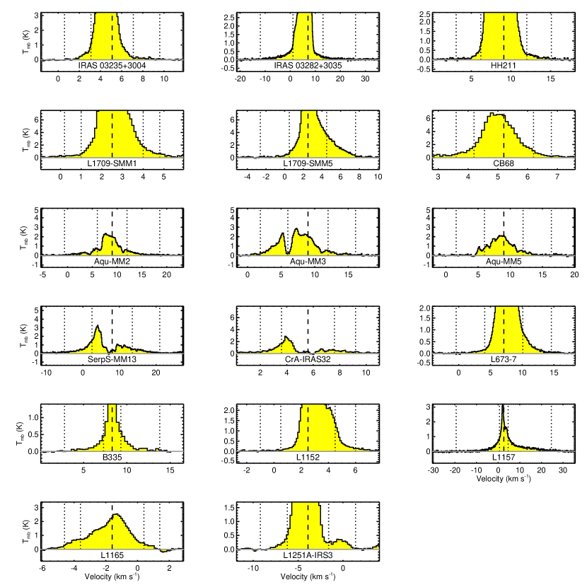
Figure 14.— Average spectra for each of the outflows mapped in ¹²CO (2–1), averaged over all spatial pixels encompassed by the outflow lobes. The dashed vertical line in each panel marks the ambient cloud velocity. The dotted vertical lines in each panel mark $v_{\rm min}$ and $v_{\rm max}$, which are chosen to be symmetrical about the cloud velocity (see §3.2 for details).

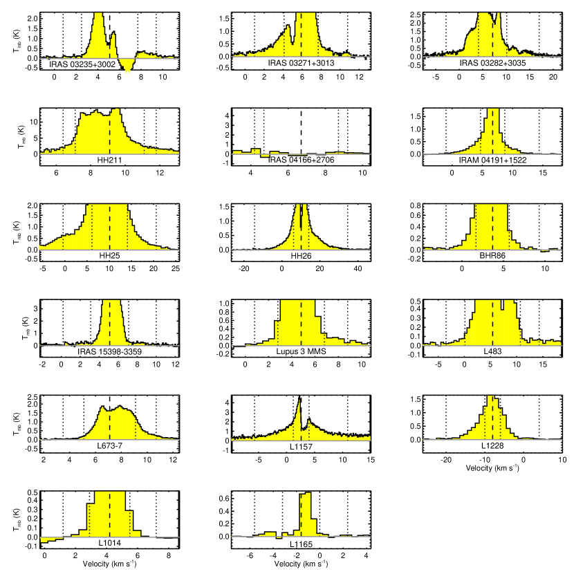
Figure 15.— Same as Figure 15, except for the outflows mapped in ¹²CO (3–2).

Appendix C C.  Optically Thin Emission from ¹²CO in LTE

C.1. C.1  Calculating Column Densities

To derive the total column density from ¹²CO observations, we first start with the definition of integrated intensity in main-beam temperature units, $\int T_{\rm mb}\,d\nu$, where $T_{\rm mb}$ is the brightness temperature of the emission:

$$\int T_{\rm mb}\,d\nu=\int\frac{c^{2}}{2\,k\,\nu^{2}}\,B_{\nu}(T)\,(1-e^{-\tau_{\nu}})\,d\nu\approx\int\frac{h\,\nu}{k}\,\frac{1}{e^{\frac{h\nu}{kT}}-1}\,\tau_{\nu}\,d\nu\,$$ (C1)

where $B_{\nu}(T)$ is the Planck function at temperature $T$, $\tau_{\nu}$ is the optical depth of the transition, and the right-most expression assumes that the emission is optically thin ($\tau_{\nu}<<1$). The optical depth of a transition from lower state J to upper state J+1 can be expressed in terms of the Einstein B coefficients for absorption ($B_{\rm J,J+1}$) and stimulated emission ($B_{\rm J+1,J}$),

$$\tau_{\rm J,J+1}=\frac{h\,\nu}{4\,\pi}\,(N_{\rm J}(\nu)\,B_{\rm J,J+1}-N_{\rm J+1}(\nu)\,B_{\rm J+1,J})\,,$$ (C2)

where $N_{\rm J}(\nu)$ and $N_{\rm J+1}(\nu)$ are the column densities in the lower and upper states, respectively. Defining $g_{\rm J}$ and $g_{\rm J+1}$ as the degeneracies of the lower and upper states, respectively, and using the relation between the Einstein B coefficients,

$$g_{\rm J+1}\,B_{\rm J+1,J}=g_{\rm J}\,B_{\rm J,J+1}\,,$$ (C3)

and the Boltzmann equation to relate $N_{\rm J}(\nu)$ and $N_{\rm J+1}(\nu)$ in LTE,

$$\frac{N_{\rm J+1}(\nu)}{N_{\rm J}(\nu)}=\frac{g_{\rm J+1}}{g_{\rm J}}\,e^{-\frac{h\,\nu}{k\,T}}\,,$$ (C4)

Equation C2 can be expressed as

$$\tau_{\rm J,J+1}=\frac{h\,\nu}{4\,\pi}\,N_{\rm J}(\nu)\,B_{\rm J,J+1}\,(1-e^{-\frac{h\,\nu}{k\,T}})\,.$$ (C5)

By using the following LTE relation between column density in a state J, $N_{\rm J}$, and total column density, $N$, where $Q(T)$ is the partition function ($Q(T)=\sum_{J=0}^{\infty}\,g_{J}\,e^{-E_{J}/kT}$),

$$N_{\rm J}(\nu)=\frac{g_{\rm J}}{Q(T)}\,e^{-\frac{E_{\rm J}}{k\,T}}\,N(\nu)\,,$$ (C6)

the optical depth of the transtion can be expressed in terms of the total column density of the molecule:

$$\tau_{\rm J,J+1}=\frac{h\,\nu}{4\,\pi}\,B_{\rm J,J+1}\,(1-e^{-\frac{h\,\nu}{k\,T}})\,\frac{g_{\rm J}}{Q(T)}\,e^{-\frac{E_{\rm J}}{k\,T}}\,N(\nu)\,.$$ (C7)

If we assume that the interval of integration in Equation C1 is much smaller than the frequency ($d\,\nu<<\nu$), such that quantities that depend on $\nu$ can be treated as constants of integration, and use the fact that the energy released by a transition from state J+1 to state J is $E_{\rm J+1,J}=h\nu=E_{\rm J+1}-E_{\rm J}$, Equation C7 can be substituted into Equation C1 to yield the expression

$$\int T_{\rm mb}\,d\nu=\frac{B_{\rm J,J+1}\,h^{2}\,\nu^{2}}{4\,\pi\,k}\,\frac{g_{\rm J}}{Q(T)}\,e^{-\frac{E_{\rm J+1}}{k\,T}}\,\int N(\nu)\,d\nu\,.$$ (C8)

Finally, recognizing that $\int N(\nu)\,d\nu$ is the total column density of the molecule, $N$, defining $X_{\rm CO}$ as the abundance of ¹²CO relative to H₂, changing the variable of integration from frequency to velocity, and using the relationship for $B_{\rm J,J+1}$ in terms of the dipole moment of the molecule $\mu$, $B_{\rm J,J+1}=\frac{32\,\pi^{4}}{3\,h^{2}\,c}\,\mu^{2}\,\frac{({\rm J}+1)}{(2{\rm J}+1)}$, the total column density of H₂ can be calculated as

$$N_{\rm H_{2}}=X_{\rm CO}\frac{3\,k}{8\,\pi^{3}\,\nu\,\mu^{2}}\frac{(2{\rm J}+1)}{({\rm J}+1)}\frac{Q(T)}{g_{\rm J}}\,e^{\frac{E_{\rm J+1}}{kT}}\int T_{\rm mb}\,dV\,.$$ (C9)

In the rest of this Appendix we will express this as $N_{\rm H_{2}}=f({\rm J},T,X_{\rm CO})\,I$, where $I$ is the integrated intensity ($I=\int T_{\rm mb}\,dV$) measured in K cm s^-1, and

$$f({\rm J},T,X_{\rm CO})=X_{\rm CO}\frac{3\,k}{8\,\pi^{3}\,\nu\,\mu^{2}}\frac{(2{\rm J}+1)}{({\rm J}+1)}\frac{Q(T)}{g_{\rm J}}\,e^{\frac{E_{\rm J+1}}{kT}}\,.$$ (C10)

C.2. C.2  Line Intensity, Column Density, and Mass Ratios For Different Excitation Temperatures

The ratio of integrated intensities in two different transitions into lower states ${\rm J_{1}}$ and ${\rm J_{2}}$, $I_{\rm J_{1}}/I_{\rm J_{2}}$, can be expressed as $f({\rm J_{2}},T,X_{\rm CO})/f({\rm J_{1}},T,X_{\rm CO})$. The correction factor to total outflow mass as a function of temperature, compared to the values obtained assuming $T=50$ K, is calculated as the ratio of column densities calculated assuming a temperature $T$ to those calculated assuming a temperature of 50 K, $N_{T}/N_{50K}=f({\rm J},T,X_{\rm CO})/f({\rm J},50K,X_{\rm CO})$. The factor by which the ratio of outflow mass calculated from two different transitions into lower states ${\rm J_{1}}$ and ${\rm J_{2}}$ will change assuming temperatures other than 50 K is then simply the ratio of the above expression calculated for both ${\rm J_{1}}$ and ${\rm J_{2}}$.

Finally, we consider the case where we have a mixture of gas at two temperatures, $T_{1}$ and $T_{2}$, with a ratio of mass (or column density) at the two temperatures $A=M_{T1}/M_{T2}=N_{T1}/N_{T2}$. Assuming the emission is optically thin and there is no self-absorption, the total measured integrated intensity is the sum of the intensity of gas at each temperature,

$$I_{\rm total}=I_{T_{1}}+I_{T_{2}}=I_{T_{1}}\,\left(1+\frac{f({\rm J},T_{1},X_{\rm CO})}{A\,f({\rm J},T_{2},X_{\rm CO})}\right)\,.$$ (C11)

The ratio of total measured integrated intensity in two different transitions with lower states ${\rm J_{1}}$ and ${\rm J_{2}}$ is then simply the ratio of Equation C11,

$$I_{\rm total,{\rm J_{1}}}/I_{\rm total,{\rm J_{2}}}=\frac{I_{T_{1},{\rm J_{1}}}}{I_{T_{1},{\rm J_{2}}}}\,\frac{\left(1+\frac{f({\rm J_{1}},T_{1},X_{\rm CO})}{A\,f({\rm J_{1}},T_{2},X_{\rm CO})}\right)}{\left(1+\frac{f({\rm J_{2}},T_{1},X_{\rm CO})}{A\,f({\rm J_{2}},T_{2},X_{\rm CO})}\right)}=\frac{f({\rm J_{2}},T_{1},X_{\rm CO})}{f({\rm J_{1}},T_{1},X_{\rm CO})}\,\frac{\left(1+\frac{f({\rm J_{1}},T_{1},X_{\rm CO})}{A\,f({\rm J_{1}},T_{2},X_{\rm CO})}\right)}{\left(1+\frac{f({\rm J_{2}},T_{1},X_{\rm CO})}{A\,f({\rm J_{2}},T_{2},X_{\rm CO})}\right)}\,.$$ (C12)

This ratio can then be used to calculate the temperature of isothermal gas in LTE that would give rise to the same line ratio, using the above expression for the ratio of integrated intensities in two different transitions.

References

- Andre et al. (1990) Andre, P., Martin-Pintado, J., Despois, D., & Montmerle, T. 1990, A&A, 236, 180
- André et al. (1999) André, P., Motte, F., & Bacmann, A. 1999, ApJ, 513, L57
- Anglada et al. (1997) Anglada, G., Sepulveda, I., & Gomez, J. F. 1997, A&AS, 121, 255
- Antoniucci et al. (2008) Antoniucci, S., Nisini, B., Giannini, T., & Lorenzetti, D. 2008, A&A, 479, 503
- Arce et al. (2010) Arce, H. G., Borkin, M. A., Goodman, A. A., Pineda, J. E., & Halle, M. W. 2010, ApJ, 715, 1170
- Arce & Goodman (2001) Arce, H. G., & Goodman, A. A. 2001, ApJ, 554, 132
- Arce et al. (2013) Arce, H. G., Mardones, D., Corder, S. A., et al. 2013, ApJ, 774, 39
- Arce et al. (2008) Arce, H. G., Santiago-García, J., Jørgensen, J. K., Tafalla, M., & Bachiller, R. 2008, ApJ, 681, L21
- Arce & Sargent (2004) Arce, H. G., & Sargent, A. I. 2004, ApJ, 612, 342
- Arce & Sargent (2006) —. 2006, ApJ, 646, 1070
- Arce et al. (2007) Arce, H. G., Shepherd, D., Gueth, F., et al. 2007, Protostars and Planets V, 245
- Bachiller (1996) Bachiller, R. 1996, ARA&A, 34, 111
- Bachiller et al. (1987) Bachiller, R., Guilloteau, S., & Kahane, C. 1987, A&A, 173, 324
- Bachiller et al. (1995) Bachiller, R., Liechti, S., Walmsley, C. M., & Colomer, F. 1995, A&A, 295, L51
- Bachiller et al. (1993) Bachiller, R., Martin-Pintado, J., & Fuente, A. 1993, ApJ, 417, L45
- Bachiller et al. (1991) Bachiller, R., Martin-Pintado, J., & Planesas, P. 1991, A&A, 251, 639
- Bachiller & Perez Gutierrez (1997) Bachiller, R., & Perez Gutierrez, M. 1997, ApJ, 487, L93
- Bachiller et al. (2001) Bachiller, R., Pérez Gutiérrez, M., Kumar, M. S. N., & Tafalla, M. 2001, A&A, 372, 899
- Bachiller et al. (1994) Bachiller, R., Terebey, S., Jarrett, T., et al. 1994, ApJ, 437, 296
- Bally et al. (1995) Bally, J., Devine, D., Fesen, R. A., & Lane, A. P. 1995, ApJ, 454, 345
- Bally et al. (1993) Bally, J., Devine, D., Hereld, M., & Rauscher, B. J. 1993, ApJ, 418, L75
- Bally & Lada (1983) Bally, J., & Lada, C. J. 1983, ApJ, 265, 824
- Bally et al. (1999) Bally, J., Reipurth, B., Lada, C. J., & Billawala, Y. 1999, AJ, 117, 410
- Banerjee et al. (2007) Banerjee, R., Klessen, R. S., & Fendt, C. 2007, ApJ, 668, 1028
- Baraffe et al. (2009) Baraffe, I., Chabrier, G., & Gallardo, J. 2009, ApJ, 702, L27
- Baraffe et al. (2012) Baraffe, I., Vorobyov, E., & Chabrier, G. 2012, ApJ, 756, 118
- Barnard et al. (1927) Barnard, E. E., Frost, E. B., & Calvert, M. R. 1927, A photographic atlas of selected regions of the Milky way
- Barranco & Goodman (1998) Barranco, J. A., & Goodman, A. A. 1998, ApJ, 504, 207
- Barsony et al. (1998) Barsony, M., Ward-Thompson, D., André, P., & O’Linger, J. 1998, ApJ, 509, 733
- Beichman et al. (1986) Beichman, C. A., Myers, P. C., Emerson, J. P., et al. 1986, ApJ, 307, 337
- Belitsky et al. (2006) Belitsky, V., Lapkin, I., Monje, R., et al. 2006, in Society of Photo-Optical Instrumentation Engineers (SPIE) Conference Series, Vol. 6275, Society of Photo-Optical Instrumentation Engineers (SPIE) Conference Series
- Belloche & André (2004) Belloche, A., & André, P. 2004, A&A, 419, L35
- Belloche et al. (2002) Belloche, A., André, P., Despois, D., & Blinder, S. 2002, A&A, 393, 927
- Benson et al. (1998) Benson, P. J., Caselli, P., & Myers, P. C. 1998, ApJ, 506, 743
- Benson & Myers (1989) Benson, P. J., & Myers, P. C. 1989, ApJS, 71, 89
- Bok & Reilly (1947) Bok, B. J., & Reilly, E. F. 1947, ApJ, 105, 255
- Bontemps et al. (1996) Bontemps, S., Andre, P., Terebey, S., & Cabrit, S. 1996, A&A, 311, 858
- Bourke et al. (2005) Bourke, T. L., Crapsi, A., Myers, P. C., et al. 2005, ApJ, 633, L129
- Bourke et al. (1995a) Bourke, T. L., Hyland, A. R., & Robinson, G. 1995a, MNRAS, 276, 1052
- Bourke et al. (1995b) Bourke, T. L., Hyland, A. R., Robinson, G., James, S. D., & Wright, C. M. 1995b, MNRAS, 276, 1067
- Buckle et al. (2009) Buckle, J. V., Hills, R. E., Smith, H., et al. 2009, MNRAS, 399, 1026
- Cabrit & Bertout (1990) Cabrit, S., & Bertout, C. 1990, ApJ, 348, 530
- Cabrit & Bertout (1992) —. 1992, A&A, 261, 274
- Caratti o Garatti et al. (2006) Caratti o Garatti, A., Giannini, T., Nisini, B., & Lorenzetti, D. 2006, A&A, 449, 1077
- Chandler & Richer (2001) Chandler, C. J., & Richer, J. S. 2001, ApJ, 555, 139
- Chapman & Mundy (2009) Chapman, N. L., & Mundy, L. G. 2009, ApJ, 699, 1866
- Chapman et al. (2007) Chapman, N. L., Lai, S.-P., Mundy, L. G., et al. 2007, ApJ, 667, 288
- Chen et al. (1997) Chen, H., Grenfell, T. G., Myers, P. C., & Hughes, J. D. 1997, ApJ, 478, 295
- Chen et al. (1995) Chen, H., Myers, P. C., Ladd, E. F., & Wood, D. O. S. 1995, ApJ, 445, 377
- Chen et al. (2012) Chen, X., Arce, H. G., Dunham, M. M., & Zhang, Q. 2012, ApJ, 747, L43
- Chen et al. (2007) Chen, X., Launhardt, R., & Henning, T. 2007, ApJ, 669, 1058
- Chen et al. (2013) Chen, X., Arce, H. G., Zhang, Q., et al. 2013, ApJ, 768, 110
- Chini et al. (2003) Chini, R., Kämpgen, K., Reipurth, B., et al. 2003, A&A, 409, 235
- Choi et al. (1995) Choi, M., Evans, II, N. J., Gregersen, E. M., & Wang, Y. 1995, ApJ, 448, 742
- Choi et al. (1993) Choi, M., Evans, II, N. J., & Jaffe, D. T. 1993, ApJ, 417, 624
- Chrysostomou et al. (2002) Chrysostomou, A., Davis, C., & Smith, M. 2002, in Revista Mexicana de Astronomia y Astrofisica Conference Series, Vol. 13, Revista Mexicana de Astronomia y Astrofisica Conference Series, ed. W. J. Henney, W. Steffen, L. Binette, & A. Raga, 16–20
- Clemens & Barvainis (1988) Clemens, D. P., & Barvainis, R. 1988, ApJS, 68, 257
- Codella & Muders (1997) Codella, C., & Muders, D. 1997, MNRAS, 291, 337
- Codella et al. (2010) Codella, C., Lefloch, B., Ceccarelli, C., et al. 2010, A&A, 518, L112
- Comerón (2008) Comerón, F. 2008, The Lupus Clouds, ed. B. Reipurth, 295
- Connelley et al. (2009) Connelley, M. S., Hodapp, K. W., & Fuller, G. A. 2009, AJ, 137, 3494
- Connelley et al. (2007) Connelley, M. S., Reipurth, B., & Tokunaga, A. T. 2007, AJ, 133, 1528
- Connelley et al. (2008) —. 2008, AJ, 135, 2496
- Crapsi et al. (2005) Crapsi, A., Caselli, P., Walmsley, C. M., et al. 2005, ApJ, 619, 379
- Cunningham et al. (2009) Cunningham, A. J., Frank, A., Carroll, J., Blackman, E. G., & Quillen, A. C. 2009, ApJ, 692, 816
- Curtis & Richer (2011) Curtis, E. I., & Richer, J. S. 2011, MNRAS, 410, 75
- Curtis et al. (2010a) Curtis, E. I., Richer, J. S., & Buckle, J. V. 2010a, MNRAS, 401, 455
- Curtis et al. (2010b) Curtis, E. I., Richer, J. S., Swift, J. J., & Williams, J. P. 2010b, MNRAS, 408, 1516
- Davis et al. (1997) Davis, C. J., Ray, T. P., Eisloeffel, J., & Corcoran, D. 1997, A&A, 324, 263
- de Geus et al. (1989) de Geus, E. J., de Zeeuw, P. T., & Lub, J. 1989, A&A, 216, 44
- Dent et al. (2000) Dent, W., Duncan, W., Ellis, M., et al. 2000, in Astronomical Society of the Pacific Conference Series, Vol. 217, Imaging at Radio through Submillimeter Wavelengths, ed. J. G. Mangum & S. J. E. Radford, 33
- Devine et al. (2009) Devine, D., Bally, J., Chiriboga, D., & Smart, K. 2009, AJ, 137, 3993
- di Francesco et al. (2007) di Francesco, J., Evans, II, N. J., Caselli, P., et al. 2007, Protostars and Planets V, 17
- Dieter (1973) Dieter, N. H. 1973, ApJ, 183, 449
- Dobashi et al. (1994) Dobashi, K., Nozawa, S., Hayashi, Y., Sato, F., & Fukui, Y. 1994, AJ, 107, 2148
- Downes & Cabrit (2007) Downes, T. P., & Cabrit, S. 2007, A&A, 471, 873
- Dunham et al. (2008) Dunham, M. M., Crapsi, A., Evans, II, N. J., et al. 2008, ApJS, 179, 249
- Dunham et al. (2010) Dunham, M. M., Evans, N. J., Bourke, T. L., et al. 2010, ApJ, 721, 995
- Dunham et al. (2006) Dunham, M. M., Evans, II, N. J., Bourke, T. L., et al. 2006, ApJ, 651, 945
- Dunham et al. (2013) Dunham, M. M., Arce, H. G., Allen, L. E., et al. 2013, AJ, 145, 94
- Eisloffel & Mundt (1997) Eisloffel, J., & Mundt, R. 1997, AJ, 114, 280
- Emprechtinger et al. (2009) Emprechtinger, M., Caselli, P., Volgenau, N. H., Stutzki, J., & Wiedner, M. C. 2009, A&A, 493, 89
- Enoch et al. (2009) Enoch, M. L., Evans, II, N. J., Sargent, A. I., & Glenn, J. 2009, ApJ, 692, 973
- Enoch et al. (2006) Enoch, M. L., Young, K. E., Glenn, J., et al. 2006, ApJ, 638, 293
- Evans et al. (2005) Evans, II, N. J., Lee, J.-E., Rawlings, J. M. C., & Choi, M. 2005, ApJ, 626, 919
- Evans et al. (2003) Evans, II, N. J., Allen, L. E., Blake, G. A., et al. 2003, PASP, 115, 965
- Evans et al. (2009) Evans, II, N. J., Dunham, M. M., Jørgensen, J. K., et al. 2009, ApJS, 181, 321
- Ezawa et al. (2004) Ezawa, H., Kawabe, R., Kohno, K., & Yamamoto, S. 2004, in Society of Photo-Optical Instrumentation Engineers (SPIE) Conference Series, Vol. 5489, Society of Photo-Optical Instrumentation Engineers (SPIE) Conference Series, ed. J. M. Oschmann, Jr., 763–772
- Frerking & Langer (1982) Frerking, M. A., & Langer, W. D. 1982, ApJ, 256, 523
- Frerking et al. (1982) Frerking, M. A., Langer, W. D., & Wilson, R. W. 1982, ApJ, 262, 590
- Froebrich et al. (2003) Froebrich, D., Smith, M. D., Hodapp, K.-W., & Eislöffel, J. 2003, MNRAS, 346, 163
- Fuller et al. (1995) Fuller, G. A., Lada, E. A., Masson, C. R., & Myers, P. C. 1995, ApJ, 453, 754
- Fuller & Myers (1993) Fuller, G. A., & Myers, P. C. 1993, ApJ, 418, 273
- Gibb & Heaton (1993) Gibb, A. G., & Heaton, B. D. 1993, A&A, 276, 511
- Gibb et al. (1995) Gibb, A. G., Little, L. T., Heaton, B. D., & Lehtinen, K. K. 1995, MNRAS, 277, 341
- Ginsburg et al. (2011) Ginsburg, A., Bally, J., & Williams, J. P. 2011, MNRAS, 418, 2121
- Goldsmith et al. (1984) Goldsmith, P. F., Snell, R. L., Hemeon-Heyer, M., & Langer, W. D. 1984, ApJ, 286, 599
- Green et al. (2013) Green, J. D., Evans, II, N. J., Jørgensen, J. K., et al. 2013, ApJ, 770, 123
- Gregersen et al. (2000) Gregersen, E. M., Evans, II, N. J., Mardones, D., & Myers, P. C. 2000, ApJ, 533, 440
- Gregersen et al. (1997) Gregersen, E. M., Evans, II, N. J., Zhou, S., & Choi, M. 1997, ApJ, 484, 256
- Gregorio Hetem et al. (1988) Gregorio Hetem, J. C., Sanzovo, G. C., & Lepine, J. R. D. 1988, A&AS, 76, 347
- Gueth & Guilloteau (1999) Gueth, F., & Guilloteau, S. 1999, A&A, 343, 571
- Gueth et al. (1997) Gueth, F., Guilloteau, S., Dutrey, A., & Bachiller, R. 1997, A&A, 323, 943
- Güsten et al. (2006) Güsten, R., Nyman, L. Å., Schilke, P., et al. 2006, A&A, 454, L13
- Gutermuth et al. (2008) Gutermuth, R. A., Bourke, T. L., Allen, L. E., et al. 2008, ApJ, 673, L151
- Gyul’Budagyan (1982) Gyul’Budagyan, A. L. 1982, Pisma v Astronomicheskii Zhurnal, 8, 232
- Haas et al. (2008) Haas, M., Heymann, F., Domke, I., et al. 2008, A&A, 488, 987
- Haikala & Laureijs (1989) Haikala, L. K., & Laureijs, R. J. 1989, A&A, 223, 287
- Hartley et al. (1986) Hartley, M., Tritton, S. B., Manchester, R. N., Smith, R. M., & Goss, W. M. 1986, A&AS, 63, 27
- Hatchell (2003) Hatchell, J. 2003, A&A, 403, L25
- Hatchell & Dunham (2009) Hatchell, J., & Dunham, M. M. 2009, A&A, 502, 139
- Hatchell et al. (2007a) Hatchell, J., Fuller, G. A., & Richer, J. S. 2007a, A&A, 472, 187
- Hatchell et al. (2007b) Hatchell, J., Fuller, G. A., Richer, J. S., Harries, T. J., & Ladd, E. F. 2007b, A&A, 468, 1009
- Hatchell et al. (2005) Hatchell, J., Richer, J. S., Fuller, G. A., et al. 2005, A&A, 440, 151
- Hatchell et al. (2012) Hatchell, J., Terebey, S., Huard, T., et al. 2012, ApJ, 754, 104
- Henning & Launhardt (1998) Henning, T., & Launhardt, R. 1998, A&A, 338, 223
- Henning et al. (1993) Henning, T., Pfau, W., Zinnecker, H., & Prusti, T. 1993, A&A, 276, 129
- Herbig (1974) Herbig, G. H. 1974, Lick Observatory Bulletin, 658, 1
- Herbig & Jones (1983) Herbig, G. H., & Jones, B. F. 1983, AJ, 88, 1040
- Heyer & Graham (1989) Heyer, M. H., & Graham, J. A. 1989, PASP, 101, 816
- Hilton & Lahulla (1995) Hilton, J., & Lahulla, J. F. 1995, A&AS, 113, 325
- Hirota et al. (1998) Hirota, T., Yamamoto, S., Mikami, H., & Ohishi, M. 1998, ApJ, 503, 717
- Hirota et al. (2008) Hirota, T., Bushimata, T., Choi, Y. K., et al. 2008, PASJ, 60, 37
- Ho et al. (2004) Ho, P. T. P., Moran, J. M., & Lo, K. Y. 2004, ApJ, 616, L1
- Hosokawa et al. (2011) Hosokawa, T., Offner, S. S. R., & Krumholz, M. R. 2011, ApJ, 738, 140
- Huard et al. (1999) Huard, T. L., Sandell, G., & Weintraub, D. A. 1999, ApJ, 526, 833
- Huard et al. (2006) Huard, T. L., Myers, P. C., Murphy, D. C., et al. 2006, ApJ, 640, 391
- Johnstone et al. (2001) Johnstone, D., Fich, M., Mitchell, G. F., & Moriarty-Schieven, G. 2001, ApJ, 559, 307
- Jørgensen et al. (2008) Jørgensen, J. K., Johnstone, D., Kirk, H., et al. 2008, ApJ, 683, 822
- Jørgensen et al. (2002) Jørgensen, J. K., Schöier, F. L., & van Dishoeck, E. F. 2002, A&A, 389, 908
- Jørgensen et al. (2009) Jørgensen, J. K., van Dishoeck, E. F., Visser, R., et al. 2009, A&A, 507, 861
- Jørgensen et al. (2006) Jørgensen, J. K., Harvey, P. M., Evans, II, N. J., et al. 2006, ApJ, 645, 1246
- Kauffmann et al. (2008) Kauffmann, J., Bertoldi, F., Bourke, T. L., Evans, II, N. J., & Lee, C. W. 2008, A&A, 487, 993
- Keene et al. (1983) Keene, J., Davidson, J. A., Harper, D. A., et al. 1983, ApJ, 274, L43
- Kenyon et al. (1994) Kenyon, S. J., Dobrzycka, D., & Hartmann, L. 1994, AJ, 108, 1872
- Kirk et al. (2006) Kirk, H., Johnstone, D., & Di Francesco, J. 2006, ApJ, 646, 1009
- Kirk et al. (2007) Kirk, H., Johnstone, D., & Tafalla, M. 2007, ApJ, 668, 1042
- Kirk et al. (2013) Kirk, H., Myers, P. C., Bourke, T. L., et al. 2013, ApJ, 766, 115
- Kirk et al. (2009) Kirk, J. M., Ward-Thompson, D., Di Francesco, J., et al. 2009, ApJS, 185, 198
- Kun (1998) Kun, M. 1998, ApJS, 115, 59
- Kun & Prusti (1993) Kun, M., & Prusti, T. 1993, A&A, 272, 235
- Lacy et al. (1994) Lacy, J. H., Knacke, R., Geballe, T. R., & Tokunaga, A. T. 1994, ApJ, 428, L69
- Lada (1985) Lada, C. J. 1985, ARA&A, 23, 267
- Ladd et al. (1993) Ladd, E. F., Lada, E. A., & Myers, P. C. 1993, ApJ, 410, 168
- Ladd et al. (1994) Ladd, E. F., Myers, P. C., & Goodman, A. A. 1994, ApJ, 433, 117
- Langer & Penzias (1993) Langer, W. D., & Penzias, A. A. 1993, ApJ, 408, 539
- Larionov et al. (1999) Larionov, G. M., Val’tts, I. E., Winnberg, A., et al. 1999, A&AS, 139, 257
- Launhardt et al. (1998) Launhardt, R., Evans, II, N. J., Wang, Y., et al. 1998, ApJS, 119, 59
- Launhardt & Henning (1997) Launhardt, R., & Henning, T. 1997, A&A, 326, 329
- Launhardt et al. (2010) Launhardt, R., Nutter, D., Ward-Thompson, D., et al. 2010, ApJS, 188, 139
- Lee et al. (2009) Lee, C.-F., Hirano, N., Palau, A., et al. 2009, ApJ, 699, 1584
- Lee et al. (2007) Lee, C.-F., Ho, P. T. P., Palau, A., et al. 2007, ApJ, 670, 1188
- Lee et al. (2005) Lee, C.-F., Ho, P. T. P., & White, S. M. 2005, ApJ, 619, 948
- Lee et al. (2002) Lee, C.-F., Mundy, L. G., Stone, J. M., & Ostriker, E. C. 2002, ApJ, 576, 294
- Lee & Myers (1999) Lee, C. W., & Myers, P. C. 1999, ApJS, 123, 233
- Lee et al. (2004) Lee, C. W., Myers, P. C., & Plume, R. 2004, ApJS, 153, 523
- Lee et al. (1999) Lee, C. W., Myers, P. C., & Tafalla, M. 1999, ApJ, 526, 788
- Lee et al. (2010) Lee, J.-E., Lee, H.-G., Shinn, J.-H., et al. 2010, ApJ, 709, L74
- Lehtinen (1997) Lehtinen, K. 1997, A&A, 317, L5
- Lehtinen & Higdon (2003) Lehtinen, K., & Higdon, J. L. 2003, A&A, 398, 583
- Lehtinen et al. (2005) Lehtinen, K., Mattila, K., & Lemke, D. 2005, A&A, 437, 159
- Lis et al. (1999) Lis, D. C., Menten, K. M., & Zylka, R. 1999, ApJ, 527, 856
- Löhr et al. (2007) Löhr, A., Bourke, T. L., Lane, A. P., et al. 2007, ApJS, 171, 478
- Lynds (1962) Lynds, B. T. 1962, ApJS, 7, 1
- Maheswar et al. (2011) Maheswar, G., Lee, C. W., & Dib, S. 2011, A&A, 536, A99
- Mardones et al. (1997) Mardones, D., Myers, P. C., Tafalla, M., et al. 1997, ApJ, 489, 719
- Margulis & Lada (1985) Margulis, M., & Lada, C. J. 1985, ApJ, 299, 925
- Masson & Chernin (1992) Masson, C. R., & Chernin, L. M. 1992, ApJ, 387, L47
- Masson & Chernin (1993) —. 1993, ApJ, 414, 230
- Matthews & Little (1983) Matthews, N., & Little, L. T. 1983, MNRAS, 205, 123
- Maury et al. (2009) Maury, A. J., André, P., & Li, Z.-Y. 2009, A&A, 499, 175
- Maury et al. (2011) Maury, A. J., André, P., Men’shchikov, A., Könyves, V., & Bontemps, S. 2011, A&A, 535, A77
- McCaughrean et al. (1994) McCaughrean, M. J., Rayner, J. T., & Zinnecker, H. 1994, ApJ, 436, L189
- Merín et al. (2008) Merín, B., Jørgensen, J., Spezzi, L., et al. 2008, ApJS, 177, 551
- Mikami et al. (1992) Mikami, H., Umemoto, T., Yamamoto, S., & Saito, S. 1992, ApJ, 392, L87
- Mitchell et al. (2001) Mitchell, G. F., Johnstone, D., Moriarty-Schieven, G., Fich, M., & Tothill, N. F. H. 2001, ApJ, 556, 215
- Miura et al. (2012) Miura, R. E., Kohno, K., Tosaki, T., et al. 2012, ApJ, 761, 37
- Morita et al. (2006) Morita, A., Watanabe, M., Sugitani, K., et al. 2006, PASJ, 58, L41
- Motte & André (2001) Motte, F., & André, P. 2001, A&A, 365, 440
- Myers et al. (1995) Myers, P. C., Bachiller, R., Caselli, P., et al. 1995, ApJ, 449, L65
- Nakamura & Li (2007) Nakamura, F., & Li, Z.-Y. 2007, ApJ, 662, 395
- Nakamura et al. (2011) Nakamura, F., Sugitani, K., Shimajiri, Y., et al. 2011, ApJ, 737, 56
- Neuhäuser & Forbrich (2008) Neuhäuser, R., & Forbrich, J. 2008, The Corona Australis Star Forming Region, ed. B. Reipurth, 735
- Nisini et al. (2002) Nisini, B., Codella, C., Giannini, T., & Richer, J. S. 2002, A&A, 395, L25
- Nutter et al. (2005) Nutter, D. J., Ward-Thompson, D., & André, P. 2005, MNRAS, 357, 975
- O’Connell et al. (2005) O’Connell, B., Smith, M. D., Froebrich, D., Davis, C. J., & Eislöffel, J. 2005, A&A, 431, 223
- Offner et al. (2011) Offner, S. S. R., Lee, E. J., Goodman, A. A., & Arce, H. 2011, ApJ, 743, 91
- Olofsson et al. (1999) Olofsson, G., Huldtgren, M., Kaas, A. A., et al. 1999, A&A, 350, 883
- Olofsson & Olofsson (2009) Olofsson, S., & Olofsson, G. 2009, A&A, 498, 455
- Palau et al. (2006) Palau, A., Ho, P. T. P., Zhang, Q., et al. 2006, ApJ, 636, L137
- Park et al. (2004) Park, Y.-S., Lee, C. W., & Myers, P. C. 2004, ApJS, 152, 81
- Park et al. (2000) Park, Y.-S., Panis, J.-F., Ohashi, N., Choi, M., & Minh, Y. C. 2000, ApJ, 542, 344
- Parker (1988) Parker, N. D. 1988, MNRAS, 235, 139
- Parker et al. (1991) Parker, N. D., Padman, R., & Scott, P. F. 1991, MNRAS, 252, 442
- Peterson et al. (2011) Peterson, D. E., Caratti o Garatti, A., Bourke, T. L., et al. 2011, ApJS, 194, 43
- Phan-Bao et al. (2011) Phan-Bao, N., Lee, C.-F., Ho, P. T. P., & Tang, Y.-W. 2011, ApJ, 735, 14
- Phan-Bao et al. (2008) Phan-Bao, N., Riaz, B., Lee, C.-F., et al. 2008, ApJ, 689, L141
- Plunkett et al. (2013) Plunkett, A. L., Arce, H. G., Corder, S. A., et al. 2013, ApJ, 774, 22
- Rebull et al. (2007) Rebull, L. M., Stapelfeldt, K. R., Evans, II, N. J., et al. 2007, ApJS, 171, 447
- Reipurth & Aspin (1997) Reipurth, B., & Aspin, C. 1997, AJ, 114, 2700
- Reipurth et al. (1997) Reipurth, B., Bally, J., & Devine, D. 1997, AJ, 114, 2708
- Reipurth et al. (1993) Reipurth, B., Chini, R., Krugel, E., Kreysa, E., & Sievers, A. 1993, A&A, 273, 221
- Risacher et al. (2006) Risacher, C., Monje, R., Vassilev, V., Pavolotsky, A., & Belitsky, V. 2006, in Society of Photo-Optical Instrumentation Engineers (SPIE) Conference Series, Vol. 6275, Society of Photo-Optical Instrumentation Engineers (SPIE) Conference Series
- Roberts et al. (2002) Roberts, H., Fuller, G. A., Millar, T. J., Hatchell, J., & Buckle, J. V. 2002, A&A, 381, 1026
- Roberts & Millar (2007) Roberts, H., & Millar, T. J. 2007, A&A, 471, 849
- Rosolowsky et al. (2008) Rosolowsky, E. W., Pineda, J. E., Foster, J. B., et al. 2008, ApJS, 175, 509
- Sandqvist (1977) Sandqvist, A. 1977, A&A, 57, 467
- Santangelo et al. (2013) Santangelo, G., Nisini, B., Antoniucci, S., et al. 2013, A&A, 557, A22
- Santiago-García et al. (2009) Santiago-García, J., Tafalla, M., Johnstone, D., & Bachiller, R. 2009, A&A, 495, 169
- Sato et al. (1994) Sato, F., Mizuno, A., Nagahama, T., et al. 1994, ApJ, 435, 279
- Schwartz et al. (1997) Schwartz, R. D., Burton, M. G., & Herrmann, J. 1997, AJ, 114, 272
- Seale & Looney (2008) Seale, J. P., & Looney, L. W. 2008, ApJ, 675, 427
- Sepúlveda et al. (2011) Sepúlveda, I., Anglada, G., Estalella, R., et al. 2011, A&A, 527, A41
- Shirley et al. (2002) Shirley, Y. L., Evans, II, N. J., & Rawlings, J. M. C. 2002, ApJ, 575, 337
- Shirley et al. (2000) Shirley, Y. L., Evans, II, N. J., Rawlings, J. M. C., & Gregersen, E. M. 2000, ApJS, 131, 249
- Shu (1977) Shu, F. H. 1977, ApJ, 214, 488
- Snell & Edwards (1982) Snell, R. L., & Edwards, S. 1982, ApJ, 259, 668
- Snell et al. (1980) Snell, R. L., Loren, R. B., & Plambeck, R. L. 1980, ApJ, 239, L17
- Sohn et al. (2007) Sohn, J., Lee, C. W., Park, Y.-S., et al. 2007, ApJ, 664, 928
- Stutz et al. (2008) Stutz, A. M., Rubin, M., Werner, M. W., et al. 2008, ApJ, 687, 389
- Tachihara et al. (1996) Tachihara, K., Dobashi, K., Mizuno, A., Ogawa, H., & Fukui, Y. 1996, PASJ, 48, 489
- Tachihara et al. (2007) Tachihara, K., Rengel, M., Nakajima, Y., et al. 2007, ApJ, 659, 1382
- Tafalla & Bachiller (1995) Tafalla, M., & Bachiller, R. 1995, ApJ, 443, L37
- Tafalla & Myers (1997) Tafalla, M., & Myers, P. C. 1997, ApJ, 491, 653
- Tafalla et al. (2000) Tafalla, M., Myers, P. C., Mardones, D., & Bachiller, R. 2000, A&A, 359, 967
- Tafalla et al. (2004) Tafalla, M., Santiago, J., Johnstone, D., & Bachiller, R. 2004, A&A, 423, L21
- Tanner & Arce (2011) Tanner, J. D., & Arce, H. G. 2011, ApJ, 726, 40
- Tobin et al. (2010) Tobin, J. J., Hartmann, L., Looney, L. W., & Chiang, H.-F. 2010, ApJ, 712, 1010
- Tobin et al. (2011) Tobin, J. J., Hartmann, L., Chiang, H.-F., et al. 2011, ApJ, 740, 45
- Tobin et al. (2013) Tobin, J. J., Chandler, C. J., Wilner, D. J., et al. 2013, ArXiv e-prints, arXiv:1310.5154
- Tomita et al. (1979) Tomita, Y., Saito, T., & Ohtani, H. 1979, PASJ, 31, 407
- Umemoto et al. (1992) Umemoto, T., Iwata, T., Fukui, Y., et al. 1992, ApJ, 392, L83
- Vallée et al. (2000) Vallée, J. P., Bastien, P., & Greaves, J. S. 2000, ApJ, 542, 352
- van der Marel et al. (2013) van der Marel, N., Kristensen, L. E., Visser, R., et al. 2013, A&A, 556, A76
- van der Tak et al. (2007) van der Tak, F. F. S., Black, J. H., Schöier, F. L., Jansen, D. J., & van Dishoeck, E. F. 2007, A&A, 468, 627
- van Kempen et al. (2009a) van Kempen, T. A., van Dishoeck, E. F., Hogerheijde, M. R., & Güsten, R. 2009a, A&A, 508, 259
- van Kempen et al. (2009b) van Kempen, T. A., van Dishoeck, E. F., Salter, D. M., et al. 2009b, A&A, 498, 167
- van Kempen et al. (2009c) van Kempen, T. A., van Dishoeck, E. F., Güsten, R., et al. 2009c, A&A, 501, 633
- van Kempen et al. (2009d) —. 2009d, A&A, 507, 1425
- Vassilev et al. (2008) Vassilev, V., Meledin, D., Lapkin, I., et al. 2008, A&A, 490, 1157
- Visser et al. (2001) Visser, A. E., Richer, J. S., & Chandler, C. J. 2001, MNRAS, 323, 257
- Visser et al. (2002) —. 2002, AJ, 124, 2756
- Wang et al. (1995) Wang, Y., Evans, II, N. J., Zhou, S., & Clemens, D. P. 1995, ApJ, 454, 217
- Watanabe et al. (2012) Watanabe, Y., Sakai, N., Lindberg, J. E., et al. 2012, ApJ, 745, 126
- Werner et al. (2004) Werner, M. W., Roellig, T. L., Low, F. J., et al. 2004, ApJS, 154, 1
- Whittet et al. (1997) Whittet, D. C. B., Prusti, T., Franco, G. A. P., et al. 1997, A&A, 327, 1194
- Wilking et al. (1992) Wilking, B. A., Greene, T. P., Lada, C. J., Meyer, M. R., & Young, E. T. 1992, ApJ, 397, 520
- Wilson et al. (2009) Wilson, T. L., Rohlfs, K., & Hüttemeister, S. 2009, Tools of Radio Astronomy (Springer-Verlag), doi:10.1007/978-3-540-85122-6
- Winnewisser (1988) Winnewisser, G. 1988, Astrophysical Letters and Communications, 26, 227
- Wu et al. (2002) Wu, J.-W., Wu, Y.-F., Wang, J.-Z., & Cai, K. 2002, Chinese J. Astron. Astrophys., 2, 33
- Wu et al. (2004) Wu, Y., Wei, Y., Zhao, M., et al. 2004, A&A, 426, 503
- Xiang & Turner (1992) Xiang, D.-L., & Turner, B. E. 1992, Chinese Astron. Astrophys., 16, 307
- Yamaguchi et al. (2012) Yamaguchi, T., Takano, S., Watanabe, Y., et al. 2012, PASJ, 64, 105
- Yıldız et al. (2013) Yıldız, U. A., Kristensen, L. E., van Dishoeck, E. F., et al. 2013, A&A, 556, A89
- Young et al. (2006) Young, C. H., Bourke, T. L., Young, K. E., et al. 2006, AJ, 132, 1998
- Young et al. (2003) Young, C. H., Shirley, Y. L., Evans, II, N. J., & Rawlings, J. M. C. 2003, ApJS, 145, 111
- Young et al. (2004) Young, C. H., Jørgensen, J. K., Shirley, Y. L., et al. 2004, ApJS, 154, 396
- Zhang et al. (1995) Zhang, Q., Ho, P. T. P., Wright, M. C. H., & Wilner, D. J. 1995, ApJ, 451, L71
- Zhou et al. (1993) Zhou, S., Evans, II, N. J., Koempe, C., & Walmsley, C. M. 1993, ApJ, 404, 232