Algebraic degrees of stretch factors in mapping class groups

Abstract

We explicitly construct pseudo-Anosov maps on the closed surface of genus $g$ with orientable foliations whose stretch factor $\lambda$ is a Salem number with algebraic degree $2g$. Using this result, we show that there is a pseudo-Anosov map whose stretch factor has algebraic degree $d$, for each positive even integer $d$ such that $d\leq g$.

1 Introduction

Let $S_{g}$ be a closed surface of genus $g\geq 2$. The mapping class group of $S_{g}$, denoted $\operatorname{Mod}(S_{g})$, is the group of isotopy classes of orientation preserving homeomorphisms of $S_{g}$. An element $f\in\operatorname{Mod}(S_{g})$ is called a pseudo-Anosov mapping class if there are transverse measured foliations $(\mathcal{F}^{u},\mu_{u})$ and $(\mathcal{F}^{s},\mu_{s})$, a number $\lambda(f)>1$, and a representative homeomorphism $\phi$ such that

$$\phi(\mathcal{F}^{u},\mu_{u})=(\mathcal{F}^{u},\lambda(f)\mu_{u})\ \ \textrm{and}\ \ \phi(\mathcal{F}^{s},\mu_{s})=(\mathcal{F}^{s},\lambda(f)^{-1}\mu_{s}).$$

In other words, $\phi$ stretches along one foliation by $\lambda(f)$ and the other by $\lambda(f)^{-1}$. The number $\lambda(f)$ is called the stretch factor (or dilatation) of $f$.

A pseudo-Anosov mapping class is said to be orientable if its invariant foliations are orientable. Let $\lambda_{H}(f)$ be the spectral radius of the action of $f$ on $H_{1}(S_{g};\R)$. Then

$$\lambda_{H}(f)\leq\lambda(f),$$

and the equality holds if and only if the invariant foliations for $f$ are orientable (see [5]). The number $\lambda_{H}(f)$ is called the homological stretch factor of $f$.

Question.

Which real numbers can be stretch factors?

It is a long-standing open question. Fried [4] conjectured that $\lambda>1$ is a stretch factor if and only if all conjugate roots of $\lambda$ and $1/\lambda$ are strictly greater than $1/\lambda$ and strictly less than $\lambda$ in magnitude.

Thurston [12] showed that a stretch factor $\lambda$ is an algebraic integer whose algebraic degree has an upper bound $6g-6$. More specifically, $\lambda$ is the largest root in absolute value of a monic palindromic polynomial. Thurston gave a construction of mapping classes of $\operatorname{Mod}(S_{g})$ generated by two multitwists and he mentioned that his construction can make a pseudo-Anosov mapping class whose stretch factor has algebraic degree $6g-6$. However, he did not give specific examples.

What happens if we fix the genus $g$? To simplify the question, we may ask which algebraic degrees are possible on $S_{g}$.

Question.

What degrees of stretch factors can occur on $S_{g}$?

Very little is known about this question. Using Thurston’s construction, it is easy to find quadratic integers as stretch factors. Neuwirth and Patterson [10] found non-quadratic examples, which are algebraic integers of degree 4 and 6 on surfaces of genus 4 and 6, respectively. Using interval exchange maps, Arnoux and Yoccoz [1] gave the first generic construction of pseudo-Anosov maps whose stretch factor has algebraic degree $g$ on $S_{g}$ for each $g\geq 2$.

Main Theorems

In this paper, we give a generic construction of pseudo-Anosov mapping classes with stretch factor of algebraic degree $2g$.

Let $c_{i}$ and $d_{j}$ be simple closed curves on $S_{g}$ as in Figure 1. For $k\geq 3$, let us define

$$f_{g,k}=T_{A_{g,k}}T_{B_{g}},$$

where $T_{A_{g,k}}=\left(T_{c_{1}}T_{c_{2}}\cdots T_{c_{g-1}}\right)\left(T_{c_{g}}\right)^{k}$ and $T_{B_{g}}=T_{d_{1}}\cdots T_{d_{g}}$. Here, $T_{\alpha}$ is the Dehn twist about $\alpha$. We will show that $f_{g,k}$ is a pseudo-Anosov mapping class and its stretch factor $\lambda(f_{g,k})$ is a special algebraic integer, called Salem number. A Salem number is an algebraic integer $\alpha>1$ whose Galois conjugates other than $\alpha$ have absolute value less than or equal to 1 and at least one conjugate lies on the unit circle.

Theorem A.

For each $g\geq 2$ and $k\geq 3$, $f_{g,k}$ is a pseudo-Anosov mapping class and satisfies the following properties:

1. $\lambda(f_{g,k})=\lambda_{H}(f_{g,k})$,

2. $\lambda(f_{g,k})$ is a Salem number, and

3. $\lim\limits_{g\rightarrow\infty}\lambda(f_{g,k})=k-1$.

2pt $S_{g}$ at 20 150 $d_{1}$ at 362 102 $c_{1}$ at 325 97 $d_{2}$ at 286 102 $c_{2}$ at 250 97 $d_{g}$ at 61 102 $c_{g}$ at 21 97

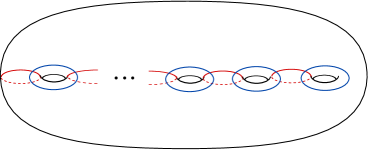
Figure 1: Simple closed curves on $S_{g}$

In particular, we will prove that for $k=4$, the algebraic degree of stretch factor is $2g$. It is known that the degree of the stretch factor of a pseudo-Anosov mapping class $f\in\operatorname{Mod}(S_{g})$ with orientable foliations is bounded above by $2g$ (see [12]). Therefore our examples give the maximum degrees of stretch factors for orientable foliations in $\operatorname{Mod}(S_{g})$ for each $g\geq 2$.

Theorem B.

Let $f_{g}\in\operatorname{Mod}(S_{g})$ be the mapping class given by

$$f_{g}=f_{g,4}=T_{A_{g,4}}T_{B_{g}}.$$

Then the minimal polynomial of the stretch factor $\lambda(f_{g})$ is

$$p_{g}(x)=x^{2g}-2\left(\sum_{j=1}^{2g-1}x^{j}\right)+1.$$

This implies

$$\deg\lambda(f_{g})=2g.$$

The hard part is to show the irreducibility of $p_{g}(x)$, which is proved in section 7.

In general, for each $k\geq 3$, the Salem stretch factor of $f_{g,k}$ is the root of the polynomial

$$p_{g,k}(x)=x^{2g}-(k-2)\left(\sum_{j=1}^{2g-1}x^{j}\right)+1.$$

It can be shown that $p_{g,k}(x)$ is irreducible for each $k\geq 4$, but since the main purpose of this paper is degree realization, we will prove only for $k=4$ case that the algebraic degree of the stretch factor is $2g$.

Using a branched cover construction, we use Theorem B to deduce the following partial answer to our question about algebraic degrees.

Corollary 5.

For each positive integer $h\leq g/2$, there is a pseudo-Anosov mapping class $\widetilde{f_{h}}\in\operatorname{Mod}(S_{g})$ such that $\deg(\lambda(\widetilde{f_{h}}))=2h$ and $\lambda(\widetilde{f_{h}})$ is a Salem number.

Obstructions.

There are three known obstructions for the existence of algebraic degrees. For any pseudo-Anosov $f\in\operatorname{Mod}(S_{g})$, we have:

1. $\deg\lambda(f)\geq 2$,

2. $\deg\lambda(f)\leq 6g-6$, and

3. if $\deg\lambda(f)>3g-3$, then $\deg\lambda(f)$ is even.

The third obstruction is due to Long [8] and we have another proof in section 5. It turns out these are the only obstructions for $g=2$. However it is not known whether there are other obstructions of algebraic degrees for $g\geq 3$. By computer search, odd degree stretch factors are rare compared to even degrees. We conjecture that every even degree $d\leq 6g-6$ can be realized as the algebraic degree of stretch factors.

Conjecture.

On $S_{g}$, there exists a pseudo-Anosov mapping class with a stretch factor of algebraic degree $d$ for each positive even integer $d\leq 6g-6$.

In section 6, we show that the conjecture is true for $g=2,3,4,$ and $5$.

Outline

In section 2 we will give the basic definitions and results about Thurston’s consturction. We will prove Theorem A in section 3 by the theory of Coxeter graphs. In section 4, we construct pseudo-Anosov mapping classes via branched covers. In section 5, we explain some properties of odd degree stretch factors. Section 6 contains examples of even degree stretch factors for $g=2,3,4$ and 5. Section 7 is where we prove Theorem B, that is, we prove that the minimal polynomial of $\lambda(f_{g})$ has degree $2g$.

Acknowledgments

I am very grateful to my advisor Dan Margalit for numerous help and discussions. I would also like to thank Joan Birman, Benson Farb, Daniel Groves, Chris Judge, and Balázs Strenner for helpful suggestions and comments. I wish to thank an anonymous referee for very helpful comments. Lastly, I would like to thank the School of Mathematics of Georgia Institute of Technology for their hospitality during the time in which the major part of this paper was made.

2 Background

Thurston’s construction

We recall Thurston’s construction of mapping classes [12]. For more details on this material, see [3] or [6].

Suppose $A=\{a_{1},\ldots,a_{n}\}$ is a set of pairwise disjoint simple closed curves, called a multicurve. We denote the product of Dehn twists $\prod_{i=1}^{n}T_{a_{i}}$ by $T_{A}$. This product is called a multitwist.

Suppose $A=\{a_{1},\ldots,a_{n}\}$ and $B=\{b_{1},\ldots,b_{m}\}$ are multicurves in a surface $S$ so that $A\cup B$ fills $S$, that is, the complement of $A\cup B$ is a disjoint union of disks and once-punctured disks. Let $N$ be the $n\times m$ matrix whose $(j,k)$-entry is the geometric intersection number $i(a_{j},b_{k})$ of $a_{j}$ and $b_{k}$. Let $\nu=\nu(A\cup B)$ be the largest eigenvalue in magnitude of the matrix $NN^{t}$. If $A\cup B$ is connected, then $NN^{t}$ is primitive and by the Perron–Frobenius theorem $\nu$ is a positive real number greater than 1 (see [3, p. 392 - 395] for more detail).

Thurston constructed a singular Euclidean structure on $S$ with respect to which $\langle T_{A},T_{B}\rangle$ acts by affine transformations given by the representation $\rho:\langle T_{A},T_{B}\rangle\rightarrow\operatorname{PSL}(2,\R)$

$$\rho(T_{A})=\left(\begin{array}[]{cc}1&-\nu^{1/2}\\ 0&1\end{array}\right)\quad\textrm{and}\quad\rho(T_{B})=\left(\begin{array}[]{cc}1&0\\ \nu^{1/2}&1\end{array}\right).$$

In particular, an element $f\in\langle T_{A},T_{B}\rangle$ is pseudo-Anosov if and only if $\rho(f)$ is a hyperbolic element in $\operatorname{PSL}(2,\R)$ and then the stretch factor $\lambda(f)$ is equal to the bigger eigenvalue of $\rho(f)$. For instance, for a mapping class $f=T_{A}T_{B}$,

$$\rho(T_{A}T_{B})=\left(\begin{array}[]{cc}1&-\nu^{1/2}\\ 0&1\end{array}\right)\left(\begin{array}[]{cc}1&0\\ \nu^{1/2}&1\end{array}\right)=\left(\begin{array}[]{cc}1-\nu&-\nu^{1/2}\\ \nu^{1/2}&1\end{array}\right),$$

and the stretch factor $\lambda(T_{A}T_{B})$ is the bigger root of the characteristic polynomial

$$\lambda^{2}-\lambda(\nu-2)+1,$$

provided that $\nu-2>2$.

3 Proof by the theory of Coxeter graphs

We will prove Theorem A in this section.

For the set $C$ of simple closed curves on the surface $S_{g}$, the configuration graph for $C$, denoted $\mathcal{G}(C)$, is the graph with a vertex for each simple closed curve and an edge for every point of intersection between simple closed curves.

Let $f_{g,k}$ be a mapping class on $S_{g}$ defined by

$$f_{g,k}=T_{A_{g,k}}T_{B_{g}},\ k\geq 3,$$

as in Theorem A. By regarding the multiple power of $T_{c_{g}}$ as the product of Dehn twists about parallel (isotopic) simple closed curves $c_{g_{1}},\ldots,c_{g_{k}}$, let us define the multicurves

$$A_{g,k}=\{c_{1},\ldots,c_{g-1},c_{g_{1}},\ldots,c_{g_{k}}\}\ \ \textrm{and}\ \ B_{g}=\{d_{1},\ldots,d_{g}\}.$$

Then the configuration graph $\mathcal{G}(A_{g,k}\cup B_{g})$ is a tree as in Figure 2,

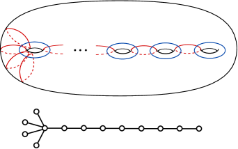
Figure 2: Multicurves and configuration graph $\mathcal{G}(A_{g,k}\cup B_{g})$

3.1 Coxeter graphs and mapping class groups

We say that a finite graph $\mathcal{G}$ is a Coxeter graph if there are no self-loops or multiple edges. For given multicurves $A$ and $B$ such that $A\cup B$ fills the surface $S$, suppose that the configuration graph $\mathcal{G}=\mathcal{G}(A\cup B)$ is a Coxeter graph. Leininger proved the following theorem.

Theorem 1 ([6] Theorem 8.1 and Theorem 8.4).

Let $\mathcal{G}(A\cup B)$ be a non-critical dominant Coxeter graph. Then $T_{A}T_{B}$ is a pseudo-Anosov mapping class with stretch factor $\lambda$ such that

$$\lambda^{2}+\lambda(2-\mu^{2})+1=0,$$

where $\mu$ is the spectral radius of the graph $\mathcal{G}$.

For the definitions and pictures of critical and dominant graphs, see [6, Section 1]

For the multicurves $A_{g,k}$ and $B_{g}$ in Theorem A, $\mathcal{G}(A_{g,k}\cup B_{g})$ is a non-critical dominant Coxeter graph for each $k\geq 3$. Therefore by Theorem 1 the mapping class $f_{g,k}=T_{A}T_{B}$ is pseudo-Anosov for each $k\geq 3$.

3.2 Orientability

Suppose that $\mathcal{G}$ is a connected Coxeter graph with the set $\Sigma$ of vertices. There is an associated quadratic form $\Pi_{\mathcal{G}}$ on $R^{\Sigma}$ and a faithful representation

$$\Theta:\mathscr{C}(\mathcal{G})\operatorname{\rightarrow}\textrm{O}(\Pi_{\mathcal{G}}),$$

where $\mathscr{C}(\mathcal{G})$ is a Coxeter group with generating set $\Sigma$, $\textrm{O}(\Pi_{\mathcal{G}})$ is the orthogonal group of the quadratic form $\Pi_{\mathcal{G}}$, and each generator $s_{i}\in\Sigma$ is represented by a reflection. Leininger also proved the following theorem.

Theorem 2 ([6] Theorem 8.2 ).

Let $\mathcal{G}(A\cup B)$ be a Coxeter graph and suppose that $A$ and $B$ can be oriented so that all intersections of $A$ with $B$ are positive. Then there exists a homomorphism

$$\eta:\R^{\Sigma}\operatorname{\rightarrow}H_{1}(S;\R)$$

such that

$$(T_{A}T_{B})_{\ast}\circ\eta=-\eta\circ\Theta(\sigma_{A}\sigma_{B}),$$

where $\sigma_{A}\sigma_{B}$ is an element in $\mathscr{C}(\mathcal{G})$ corresponding to $T_{A}T_{B}$.
Moreover, $\Theta(\sigma_{A}\sigma_{B})|_{\textrm{ker}(\eta)}=-I$ and $\eta$ preserves spectral radii.

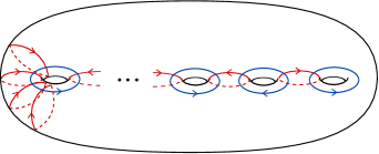
Figure 3: Orientation of positive intersections

Theorem 2 implies that if $A$ and $B$ can be oriented as in the theorem, then the stretch factor of a pseudo-Anosov mapping class is equal to the spectral radius of the action on homology. For multicurves $A_{g,k}$ and $B_{g}$ in Theorem A, they can be oriented so that all intersections are positive as in Figure 3. Therefore we have

$$\lambda(f_{g,k})=\lambda_{H}(f_{g,k})$$

and the invariant foliations for $f_{g,k}$ are orientable.

It is also possible to directly compute the action on the first homology. Consider the mapping class $f_{g}=T_{A_{g,4}}T_{B_{g}}$ as in Theorem B. Let us choose a basis $\{a_{1},b_{1},\dots,a_{g},b_{g}\}$ for $H_{1}(S_{g})$ as in Figure 4.

2pt $S_{g}$ at 20 150 $a_{1}$ at 362 100 $b_{1}$ at 325 100 $a_{2}$ at 286 100 $b_{2}$ at 250 100 $a_{3}$ at 210 100 $a_{g}$ at 61 100 $b_{g}$ at 21 100

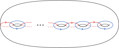
Figure 4: A basis for $H_{1}(S_{g})$.

By computing images of each basis element under $f_{g}$, we can get the action on $H_{1}(S_{g})$

$$\left(\begin{array}[]{rrrrcr}1&-1&0&~{}0&\cdots&0\\ 1&0&-1&0&\cdots&0\\ \vdots&\vdots&\vdots&\vdots&\ddots&\vdots\\ 1&0&0&0&\cdots&-1\\ 4&0&0&0&\cdots&-3\end{array}\right).$$

By induction, the characteristic polynomial $h_{g}(x)$ of the homological action is

$$h_{g}(x)=x^{2g}+2\left(\sum_{j=1}^{2g-1}(-1)^{j}x^{j}\right)+1.$$

Since the largest root of $h_{g}(x)$ in magnitude is a negative real number, we can deduce that the stretch factor $\lambda(f_{g})$ is the root of $h_{g}(-x)$. Specifically, $\lambda(f_{g})$ is the root of

$$p_{g}(x)=x^{2g}-2\left(\sum_{j=1}^{2g-1}x^{j}\right)+1.$$

In a similar way, one can get the polynomial for $\lambda(f_{g,k})$, which is

$$p_{g,k}(x)=x^{2g}-(k-2)\left(\sum_{j=1}^{2g-1}x^{j}\right)+1.$$

3.3 Salem numbers and spectral properties of starlike trees

The configuration graph $\mathcal{G}(A_{g,k}\cup B_{g})$ for $f_{g,k}$ is a special type of graphs, called a starlike tree, and its relation to Salem numbers is studied in [9]. A starlike tree is a tree with at most one vertex of degree $>2$. Let $T=T(n_{1},n_{2},\ldots,n_{k})$ be the starlike tree with $k$ arms of $n_{1},n_{2},\ldots,n_{k}$ edges.

Theorem 3 ([9] Corollary 9).

Let $T=T(n_{1},n_{2},\ldots,n_{k})$ be a starlike tree and let $\mu$ be the spectral radius of $T$. Suppose that $\mu$ is not an integer and $T$ is a non-critical dominant graph. Then $\lambda>1$, defined by $\sqrt{\lambda}+1/\sqrt{\lambda}=\mu$, is a Salem number.

The configuration graph $\mathcal{G}(A_{g,k}\cup B_{g})$ in Theorem A is a non-critical dominant starlike tree

$$T(2g-2,\underbrace{1,1,\ldots,1}_{k\textrm{-times}}),\ k\geq 3$$

and we will denote it by $T(2g-2,k\cdot 1$). The fact that the spectral radius of $T(2g-2,k\cdot 1)$ is not an integer follows from the following theorem.

Theorem 4 ([11]).

If $\mu$ is the spectral radius of the starlike tree $T(n,k\cdot 1)$, then

$$\sqrt{k+1}<\mu<\frac{k}{\sqrt{k-1}}$$

for $n\geq 1$ and $k\geq 3$.

Thus for the starlike tree $T(n,k\cdot 1)$, the spectral radius satisfies

$$k+1<\mu^{2}<\frac{k^{2}}{k-1}=k+1+\frac{1}{k-1}.$$

Therefore $\mu$ is not an integer and by Theorem 3 $\lambda(f_{g,k})$ is a Salem number.

Moreover, the proof of Corollary 2.1 of Lepović–Gutman [7] implies that

$$\lim\limits_{g\rightarrow\infty}\lambda(f_{g,k})=k-1.$$

For completeness, we reprove this here.

Recall that $\lambda(f_{g,k})$ is the largest root of

$$p_{g,k}(x)=x^{2g}-(k-2)\left(\sum_{j=1}^{2g-1}x^{j}\right)+1.$$

By multiplying $p_{g,k}(x)$ by $x-1$, the stretch factor $\lambda(f_{g,k})$ is the largest root in magnitude of

$$q_{g,k}(x)=x^{2g+1}-(k-1)x^{2g}+(k-1)x-1.$$

We have $q_{g,k}(k-1)=(k-1)^{2}-1>0$, and for any fixed positive integer $m$,

$$q_{g,k}\left(k-1-\frac{1}{10^{m}}\right) = \left(k-1-\frac{1}{10^{m}}\right)^{2g}\left(-\frac{1}{10^{m}}\right)+(k-1)\left(k-1-\frac{1}{10^{m}}\right)-1$$

Hence $q_{g,k}\left(k-1-10^{-m}\right)<0$ for sufficiently large values of $g$ and therefore $p_{g,k}(x)$ has a root on the interval $(k-1-10^{-m},k-1)$. This implies

$$\lim\limits_{g\rightarrow\infty}\lambda(f_{g,k})=k-1.$$

This completes the proof of Theorem A.

Remark.

A positive integer cannot be a stretch factor (which is an algebraic integer of degree 1). However, Theorem A implies that for sufficiently large genus $g$ there is a stretch factor which is a Salem number arbitrarily close to a given integer $k-1$ for each $k\geq 3$.

4 Branched Covers

Lifting a pseudo-Anosov mapping class via a covering map is one way to construct another pseudo-Anosov mapping class. If there is a branched cover $\widetilde{S}\rightarrow S$ and a pseudo-Anosov mapping class $f\in\operatorname{Mod}(S)$, then there is some $k\in\mathbb{N}$ such that $\operatorname{Mod}(\widetilde{S})$ has a pseudo-Anosov element $\widetilde{f}$ which is a lift of $f^{k}$ and hence $\lambda(\widetilde{f})=\lambda(f)^{k}$.

Corollary 5.

Let $g\geq 2$. For each positive integer $h\leq g/2$, there is a pseudo-Anosov mapping class $\widetilde{f_{h}}\in\operatorname{Mod}(S_{g})$ such that $\deg(\lambda(\widetilde{f_{h}}))=2h$ and $\lambda(\widetilde{f_{h}})$ is a Salem number.

Proof.

Let

$$h=\left\{\begin{array}[]{ll}\frac{g-2m}{2},&\textrm{if $g$ is even, $m=0,1,\ldots,(g-2)/2$,}\\ &\\ \frac{g-1-2m}{2},&\textrm{if $g$ is odd, $m=0,1,\ldots,(g-3)/2$.}\end{array}\right.$$

Then $h$ is an integer such that $1\leq h\leq g/2$.

2pt $S_{g}$ [l] at 22 350 $S_{g}$ [l] at 298 350 $S_{h}$ [l] at 40 126 $S_{h}$ [l] at 318 126 $g$ even at 114 10 $g$ odd at 393 13

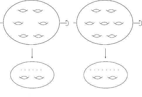
Figure 5: A branched cover

Construct a branched cover $S_{g}\rightarrow S_{h}$ as in Figure 5. For $h\geq 2$, $S_{h}$ has a pseudo-Anosov mapping class $f_{h}\in\operatorname{Mod}(S_{h})$ as in the Theorem B whose stretch factor has $\deg(\lambda(f_{h}))=2h$. For some $k$, ${f_{h}}^{k}$ lifts to $S_{g}$ and the lift has stretch factor $\lambda(f_{h})^{k}$. We claim that $\deg\left(\lambda(f_{h})^{k}\right)=2h$. To see this, let $\lambda_{i}$, $1\leq i\leq 2h$, be the roots of the minimal polynomial of $\lambda(f_{h})$ and let us define a polynomial

$$p(x)=\prod_{i=1}^{2h}\left(x-\lambda_{i}^{k}\right).$$

Then $p(x)$ is an integral polynomial because the following elementary symmetric polynomials in $\lambda_{1},\ldots,\lambda_{2h}$

$$\sum\lambda_{i},\ \sum_{i<j}\lambda_{i}\lambda_{j},\ \sum_{i<j<l}\lambda_{i}\lambda_{j}\lambda_{l},\ \cdots,\ \lambda_{1}\lambda_{2}\cdots\lambda_{2h}$$

are all integers and hence each coefficient of $p(x)$

$$\sum\lambda_{i}^{k},\ \sum_{i<j}\lambda_{i}^{k}\lambda_{j}^{k},\ \sum_{i<j<l}\lambda_{i}^{k}\lambda_{j}^{k}\lambda_{l}^{k},\ \cdots,\ \lambda_{1}^{k}\lambda_{2}^{k}\cdots\lambda_{2h}^{k}$$

are integers as well. Therefore $p(x)$ is divided by the minimal polynomial of $\lambda(f_{h})^{k}$. Due to the proof of Theorem B in section 7, $\lambda(f_{h})^{k}$ is also a Salem number and $p(x)$ does not have a cyclotomic factor. This implies that $p(x)$ is irreducible and $\deg\left(\lambda(f_{h})^{k}\right)=2h$.

If $h=1$, $S_{h}$ is a torus and it admits a Anosov mapping class $f$ whose stretch factor $\lambda(f)$ has algebraic degree $2$. Then similar arguments as above tells us that there is a lift of some power of $f$ to $S_{g}$ whose stretch factor has $\deg(\lambda(f^{k}))=2$.

Therefore there is a pseudo-Anosov map $\widetilde{f_{h}}\in\operatorname{Mod}(S_{g})$ with $\deg(\lambda(\widetilde{f_{h}}))=2h$ for each $h\leq g/2$. In other words, every positive even degree $d\leq g$ is realized as the algebraic degree of a stretch factor on $S_{g}$. ∎

5 Stretch factors of odd degrees

Long proved the following degree obstruction and McMullen communicated to us the following proof. First we will give a definition of the reciprocal polynomial. Given a polynomial $p(x)$ of degree $d$, we define the reciprocal polynomial $p^{*}(x)$ of $p(x)$ by $p^{*}(x)=x^{d}p(1/x)$. It is a well-known property that $p^{*}(x)$ is irreducible if and only if $p(x)$ is irreducible.

Theorem 6 ([8]).

Let $f\in\operatorname{Mod}(S_{g})$ be a pseudo-Anosov mapping class having stretch factor $\lambda(f)$. If $\deg(\lambda(f))>3g-3$, then $\deg(\lambda(f))$ is even.

Proof.

Since $f$ acts by a piecewise integral projective transformation on the $6g-6$ dimensional space $\operatorname{\mathcal{PMF}}$ of projective measured foliations on $S_{g}$, and since $\lambda(f)$ is an eigenvalue of this action, $\lambda(f)$ is an algebraic integer with $\deg(\lambda(f))\leq 6g-6$. Also, since $f$ preserves the symplectic structure on $\operatorname{\mathcal{PMF}}$, it follows that $\lambda(f)$ is the root of palindromic polynomial $p(x)$ whose degree is bounded above by $6g-6$.

Let $q(x)$ be the minimal polynomial of $\lambda(f)$ and let $q^{*}(x)$ be the reciprocal polynomial of $q(x)$. Then either $q(x)=q^{*}(x)$ or they have no common roots, because if there is at least one common root $\zeta$ of $q(x)$ and $q^{*}(x)$, then both $q(x)$ and $q^{*}(x)$ are the minimal polynomial of $\zeta$ and hence $q(x)=q^{*}(x)$. Suppose $\deg(q(x))>3g-3$. If $q(x)$ and $q^{*}(x)$ have no common roots, then their product $q(x)\,q^{*}(x)$ is a factor of $p(x)$ since $q^{*}(x)$ is the minimal polynomial of $1/\lambda(f)$. This is a contradiction because $\deg(p(x))\leq 6g-6$ but $\deg\big{(}q(x)\,q^{*}(x)\big{)}>6g-6$. Therefore we must have $q(x)=q^{*}(x)$ and this implies that $q(x)$ is an irreducible palindromic polynomial. Hence $\deg(q(x))$ is even since roots of $q(x)$ come in pairs, $\lambda_{i}$ and $1/\lambda_{i}$. ∎

It follows from the previous proof that if the minimal polynomial $p(x)$ of $\lambda$ has odd degree, then $p(x)$ is not palindromic and in fact the minimal palindromic polynomial containing $\lambda$ as a root is $p(x)p^{*}(x)$.

We will now show that the stretch factors of degree 3 have an additional special property. A Pisot number, also called a Pisot–Vijayaraghavan number or a PV number, is an algebraic integer greater than 1 such that all its Galois conjugates are strictly less than 1 in absolute value.

Proposition 7.

Let $f\in\operatorname{Mod}(S_{g})$. If $\deg(\lambda(f))=3$, then $\lambda(f)$ is a Pisot number.

Proof.

Let $\lambda_{1}>1$ be the stretch factor of a pseudo-Anosov mapping class with algebraic degree 3, and let $p(x)$ be the minimal polynomial of $\lambda_{1}$. Let $\lambda_{1},\lambda_{2},$ and $\lambda_{3}$ be the roots of $p(x)$. Then the degree of $p(x)p^{*}(x)$ is 6 and it has pairs of roots $(\lambda_{1},1/\lambda_{1}),(\lambda_{2},1/\lambda_{2}),(\lambda_{3},1/\lambda_{3})$, where $\lambda_{1}$ is the largest root in absolute value. We claim that the absolute values of $\lambda_{2}$ and $\lambda_{3}$ are strictly less than 1.

Suppose one of them has absolute value greater than or equal to 1, say $|\lambda_{2}|\geq 1$. The constant term $\lambda_{1}\lambda_{2}\lambda_{3}$ of $p(x)$ is $\pm 1$ since it is the factor of a palindromic polynomial with constant term 1. Hence $|\lambda_{1}\lambda_{2}\lambda_{3}|=1$ and we have

$$\frac{1}{|\lambda_{3}|}=|\lambda_{1}\lambda_{2}|\geq|\lambda_{1}|,$$

which is a contradiction to the fact that the stretch factor $\lambda_{1}$ is strictly greater than all other roots of the palindromic polynomial $p(x)p^{*}(x)$. This proves the claim and hence the stretch factor of degree 3 is a Pisot number. ∎

We now explain two constructions of mapping classes $f\in\operatorname{Mod}(S_{g})$ whose degree of $\lambda(f)$ is odd.

1. As we mentioned, Arnoux–Yoccoz [1] gave examples of a pseudo-Anosov mapping class on $S_{g}$ whose stretch factor has algebraic degree $g$. In particular for odd $g$, this gives examples of mapping classes with odd degree stretch factors. They proved that these stretch factors are all Pisot numbers.

2. For genus $2$, there is a pseudo-Anosov mapping class $f$ whose stretch factor has algebraic degree 3 (see section 6). This is the only possible odd degree on $S_{2}$ by Long’s obstruction. It is also true that $\deg(\lambda(f)^{k})=3$ for each $k$ because the stretch factor is a Pisot number (Proposition 7). There is a cover $S_{g}\rightarrow S_{2}$ for each $g$, so the lift of some power of $f$ has a stretch factor with algebraic degree 3 on $S_{g}$.

Proposition 8.

For each genus $g$, the stretch factor with algebraic degree 3 can occur on $S_{g}$.

Question.

Are there stretch factors with odd algebraic degree that are not Pisot numbers?

6 Examples of even degrees

Tables 1 through 4 give explicit examples of pseudo-Anosov mapping classes whose stretch factors realize various degrees. We will follow the notation of the software Xtrain by Brinkmann. More specifically, $a_{i},b_{i},c_{i},$ and $d_{i}$ are Dehn twists along standard curves and $A_{i},B_{i},C_{i},$ and $D_{i}$ are the inverse twists as in [2]. The only missing degree on $S_{3}$ is degree 5. We do not know if there is a degree 5 example or there is another degree obstruction.

deg	$\hskip 5.40005ptf\in\operatorname{Mod}(S_{2})$	Minimal polynomial	$\lambda(f)$
2	$a_{0}a_{0}d_{0}C_{0}D_{1}C_{0}$	$x^{2}-3x+1$	$\lambda=2.618$
3	$a_{0}d_{0}d_{0}C_{0}C_{0}D_{1}$	$x^{3}-3x^{2}-x-1$	$\lambda=3.383$
4	$a_{0}d_{0}d_{0}d_{1}c_{0}d_{0}$	$x^{4}-x^{3}-x^{2}-x+1$	$\lambda=1.722$
6	$a_{0}a_{0}d_{0}A_{0}C_{0}D_{1}$	$x^{6}-x^{5}-4x^{3}-x+1$	$\lambda=2.015$

Table 1: Examples of genus 2

deg	$\hskip 9.00002ptf\in\operatorname{Mod}(S_{3})$	Minimal polynomial	$\lambda(f)$
2	$a_{1}c_{0}d_{0}c_{0}d_{2}C_{1}D_{1}$	$x^{2}-4x+1$	$3.732$
3	$a_{0}c_{0}d_{0}C_{1}D_{1}D_{2}$	$x^{3}-2x^{2}+x-1$	$1.755$
4	$a_{1}c_{0}d_{0}a_{1}c_{1}d_{1}d_{2}$	$x^{4}-x^{3}-2x^{2}-x+1$	$1.722$
6	$a_{0}c_{0}d_{0}d_{2}C_{1}D_{1}$	$x^{6}-3x^{5}+3x^{4}-7x^{3}+3x^{2}-3x+1$	$2.739$
8	$a_{0}c_{0}d_{0}d_{1}C_{1}D_{2}$	$x^{8}-x^{7}-2x^{5}-2x^{3}-x+1$	$1.809$
10	$a_{1}c_{0}d_{0}d_{1}C_{1}A_{2}D_{2}$	$x^{10}-x^{9}-2x^{8}+2x^{7}-2x^{5}+2x^{3}-2x^{2}-x+1$	$1.697$
12	$a_{1}c_{1}c_{0}d_{1}d_{2}A_{0}D_{0}$	$x^{12}-x^{11}-x^{9}-x^{8}+x^{7}+x^{5}-x^{4}-x^{3}-x+1$	$1.533$

Table 2: Examples of genus 3

deg	$\hskip 14.40007ptf\in\operatorname{Mod}(S_{4})$	deg	$\hskip 14.40007ptf\in\operatorname{Mod}(S_{4})$
4	$a_{0}a_{0}a_{1}c_{0}d_{0}c_{1}d_{1}c_{2}d_{2}c_{3}d_{3}$	12	$a_{0}B_{1}d_{0}c_{0}d_{1}c_{1}d_{2}c_{2}d_{3}c_{3}$
6	$a_{0}B_{2}A_{3}d_{0}c_{0}d_{1}c_{1}d_{2}c_{2}d_{3}c_{3}$	14	$a_{0}d_{0}B_{0}d_{0}c_{0}d_{1}c_{1}d_{2}c_{2}d_{3}c_{3}$
8	$a_{0}A_{1}d_{0}c_{0}d_{1}c_{1}d_{2}c_{2}d_{3}c_{3}$	16	$A_{0}d_{0}c_{0}d_{1}c_{1}d_{2}c_{2}d_{3}c_{3}$
10	$a_{0}b_{1}A_{2}d_{0}c_{0}d_{1}c_{1}d_{2}c_{2}d_{3}c_{3}$	18	$a_{0}B_{1}A_{2}d_{0}c_{0}d_{1}c_{1}d_{2}c_{2}d_{3}c_{3}$

Table 3: Examples of genus 4

deg	$\hskip 18.00003ptf\in\operatorname{Mod}(S_{5})$	deg	$\hskip 18.00003ptf\in\operatorname{Mod}(S_{5})$
6	$b_{3}d_{0}c_{0}d_{1}c_{1}d_{2}c_{2}d_{3}c_{3}d_{4}c_{4}$	16	$a_{1}B_{2}d_{0}c_{0}d_{1}c_{1}d_{2}c_{2}d_{3}c_{3}d_{4}c_{4}$
8	$a_{0}a_{1}d_{0}c_{0}d_{1}c_{1}d_{2}c_{2}d_{3}c_{3}d_{4}c_{4}$	18	$a_{1}B_{0}d_{0}c_{0}d_{1}c_{1}d_{2}c_{2}d_{3}c_{3}d_{4}c_{4}$
10	$a_{1}A_{4}d_{0}c_{0}d_{1}c_{1}d_{2}c_{2}d_{3}c_{3}d_{4}c_{4}$	20	$a_{1}A_{0}d_{0}c_{0}d_{1}c_{1}d_{2}c_{2}d_{3}c_{3}d_{4}c_{4}$
12	$b_{2}C_{2}d_{0}c_{0}d_{1}c_{1}d_{2}c_{2}d_{3}c_{3}d_{4}c_{4}$	22	$a_{2}A_{1}d_{0}c_{0}d_{1}c_{1}d_{2}c_{2}d_{3}c_{3}d_{4}c_{4}$
14	$a_{1}B_{1}d_{0}c_{0}d_{1}c_{1}d_{2}c_{2}d_{3}c_{3}d_{4}c_{4}$	24	$c_{2}A_{2}d_{0}c_{0}d_{1}c_{1}d_{2}c_{2}d_{3}c_{3}d_{4}c_{4}$

Table 4: Examples of genus 5

7 Irreducibility of Polynomials

In this section, we will prove Theorem B. It is enough to show that the polynomial

$$p_{n}(x)=x^{2n}-2\left(\sum_{j=1}^{2n-1}x^{j}\right)+1.$$

is irreiducible for $n\geq 2$. We will show that $p_{n}(x)$ does not have a cyclotomic polynomial factor. It then follows from Kronecker’s theorem that $p_{n}(x)$ is irreducible.

Suppose $p_{n}(x)$ has the $m$th cyclotomic polynomial factor for some $m\in\mathbb{N}$. Then $e^{2\pi i/m}$ is a root of $p_{n}(x)$. Multiplying $p_{n}(x)$ by $x-1$ yields

$$x^{2n+1}-3x^{2n}+3x-1$$

and hence we have

(1) $$\ e^{2(2n+1)\pi i/m}-3e^{4n\pi i/m}+3e^{2\pi i/m}-1=0.$$

Consider the real part and the complex part of (1). Then we have the system of equations

$$\left\{\begin{array}[]{l}\cos\big{(}\frac{2(2n+1)\pi}{m}\big{)}-3\cos\big{(}\frac{4n\pi}{m}\big{)}+3\cos\big{(}\frac{2\pi}{m}\big{)}-1=0\\ \sin\big{(}\frac{2(2n+1)\pi}{m}\big{)}-3\sin\big{(}\frac{4n\pi}{m}\big{)}+3\sin\big{(}\frac{2\pi}{m}\big{)}=0\\ \end{array}\right.$$

Using double-angle formula for the first cosine and sum-to-product formula for the last two cosines, the first equation gives

$$2\sin\Big{(}\frac{(2n+1)\pi}{m}\Big{)}\Big{[}3\sin\Big{(}\frac{(2n-1)\pi}{m}\Big{)}-\sin\Big{(}\frac{(2n+1)\pi}{m}\Big{)}\Big{]}=0.$$

Similarly the second equation gives

$$2\cos\Big{(}\frac{(2n+1)\pi}{m}\Big{)}\Big{[}\sin\Big{(}\frac{(2n+1)\pi}{m}\Big{)}-3\sin\Big{(}\frac{(2n-1)\pi}{m}\Big{)}\Big{]}=0.$$

Since sine and cosine have no common zeros, we must have

$$\sin\Big{(}\frac{(2n+1)\pi}{m}\Big{)}-3\sin\Big{(}\frac{(2n-1)\pi}{m}\Big{)}=0.$$

For $m\leq 5$, by direct calculation we can see that $p_{n}(e^{2\pi i/m})\neq 0$. So we may assume that $m\geq 6$. Let $\varphi=(2n-1)\pi/m$ and then we can write the above equation as

(2) $$\sin\Big{(}\varphi+\frac{2\pi}{m}\Big{)}-3\sin(\varphi)=0.$$

Since $\sin\big{(}\varphi+2\pi/m\big{)}$ is a real number between $-1$ and $1$, we have

(3) $$-\frac{1}{3}\leq\sin(\varphi)\leq\frac{1}{3}.$$

Let $\psi=\sin^{-1}(1/3)$. Then note that $\psi<\pi/6$. Equation (3) gives the restriction on $\varphi$, which is

$$-\psi\leq\varphi\leq\psi\ \ \textrm{or}\ \ \pi-\psi\leq\varphi\leq\pi+\psi.$$

Another observation from (2) is that both $\sin\big{(}\varphi+2\pi/m\big{)}$ and $\sin(\varphi)$ must have the same sign.

We claim that $\varphi$ has to be on the either first or third quadrant. Suppose $\varphi$ is on the second quadrant, that is, $\pi-\psi<\varphi<\pi$. Note that $m\geq 6$ implies $2\pi/m\leq\pi/3$. Since $\varphi$ is above the $x$-axis, $\varphi+2\pi/m$ also has to be above the $x$-axis due to (2) and hence the only possibility is that $\varphi+2\pi/m$ is between $\varphi$ and $\pi$. Then

$$0<\sin\Big{(}\varphi+\frac{2\pi}{m}\Big{)}<\sin(\varphi)\ \implies\ \sin\Big{(}\varphi+\frac{2\pi}{m}\Big{)}<3\sin(\varphi),$$

which is a contradiction to (2). Similar arguments hold if $\varphi$ is on the fourth quadrant. Therefore the possible range for $\varphi$ is

$$0<\varphi\leq\psi\ \ \textrm{or}\ \ \pi<\varphi\leq\pi+\psi.$$

Suppose $\varphi$ is on the first quadrant. Then so is $\varphi+2\pi/m$ because

$$0<\varphi+\frac{2\pi}{m}\leq\psi+\frac{\pi}{3}<\frac{\pi}{2}.$$

We can write

$$\varphi=\frac{(2n-1)\pi}{m}\equiv\ \frac{j\pi}{m}\pmod{2\pi}$$

for some positive integer $j$, i.e., $0<j\pi/m<\pi/2$.

If $j\geq 2$, Using the subadditivity of $\sin(x)$ on the first quadrant

$$\sin(x+y)\leq\sin(x)+\sin(y),$$

we have

$$\sin\Big{(}\varphi+\frac{2\pi}{m}\Big{)}-3\sin(\varphi) \leq \left(\sin(\varphi)+\sin\Big{(}\frac{2\pi}{m}\Big{)}\right)-3\sin(\varphi)$$

$$= \sin\Big{(}\frac{2\pi}{m}\Big{)}-2\sin(\varphi)$$

$$= \sin\Big{(}\frac{2\pi}{m}\Big{)}-2\sin\Big{(}\frac{j\pi}{m}\Big{)}<0,$$

which contradicts (2).

If $j=1$, using triple-angle formula

$$\sin\Big{(}\varphi+\frac{2\pi}{m}\Big{)}-3\sin(\varphi) = \sin\Big{(}\frac{3\pi}{m}\Big{)}-3\sin\Big{(}\frac{\pi}{m}\Big{)}$$

$$= \left(3\sin\Big{(}\frac{\pi}{m}\Big{)}-4\sin^{3}\Big{(}\frac{\pi}{m}\Big{)}\right)-3\sin\Big{(}\frac{\pi}{m}\Big{)}$$

$$= -4\sin^{3}\Big{(}\frac{\pi}{m}\Big{)}<0,$$

which contradicts (2) again. Therefore there is no possible $\varphi$ on the first quadrant. By using the same arguments, the fact that $\varphi$ is on the third quadrant gives a contradiction. Therefore we can conclude that $p(x)$ does not have a cyclotomic factor.

We now show that $p_{n}(x)$ is irreducible over $\Z$. Suppose $p_{n}(x)$ is reducible and write $p_{n}(x)=g(x)h(x)$ with non-constant functions $g(x)$ and $h(x)$. There is only one root of $p_{n}(x)$ whose absolute value is strictly greater than 1. Therefore one of $g(x)$ or $h(x)$ has all roots inside the unit disk. By Kronecker’s theorem, this polynomial has to be a product of cyclotomic polynomials, which is a contradiction because $p_{n}(x)$ does not have a cyclotomic polynomial factor. Therefore $p_{n}(x)$ is irreducible.

References

- [1] Pierre Arnoux and Jean-Christophe Yoccoz. Construction de difféomorphismes pseudo-Anosov. C. R. Acad. Sci. Paris Sér. I Math., 292(1):75–78, 1981.
- [2] Peter Brinkmann. An implementation of the Bestvina-Handel algorithm for surface homeomorphisms. Experiment. Math., 9(2):235–240, 2000.
- [3] Benson Farb and Dan Margalit. A primer on mapping class groups, volume 49 of Princeton Mathematical Series. Princeton University Press, Princeton, NJ, 2012.
- [4] David Fried. Growth rate of surface homeomorphisms and flow equivalence. Ergodic Theory Dynam. Systems, 5(4):539–563, 1985.
- [5] Erwan Lanneau and Jean-Luc Thiffeault. On the minimum dilatation of pseudo-Anosov homeromorphisms on surfaces of small genus. Ann. Inst. Fourier (Grenoble), 61(1):105–144, 2011.
- [6] Christopher J. Leininger. On groups generated by two positive multi-twists: Teichmüller curves and Lehmer’s number. Geom. Topol., 8:1301–1359 (electronic), 2004.
- [7] M. Lepović and I. Gutman. Some spectral properties of starlike trees. Bull. Cl. Sci. Math. Nat. Sci. Math., (26):107–113, 2001. The 100th anniversary of the birthday of Academician Jovan Karamata.
- [8] D. D. Long. Constructing pseudo-Anosov maps. In Knot theory and manifolds (Vancouver, B.C., 1983), volume 1144 of Lecture Notes in Math., pages 108–114. Springer, Berlin, 1985.
- [9] J. F. McKee, P. Rowlinson, and C. J. Smyth. Salem numbers and Pisot numbers from stars. In Number theory in progress, Vol. 1 (Zakopane-Kościelisko, 1997), pages 309–319. de Gruyter, Berlin, 1999.
- [10] L. Neuwirth and N. Patterson. A sequence of pseudo-Anosov diffeomorphisms. In Combinatorial group theory and topology (Alta, Utah, 1984), volume 111 of Ann. of Math. Stud., pages 443–449. Princeton Univ. Press, Princeton, NJ, 1987.
- [11] Hyunshik Shin. Spectral radius of starlike trees with one long arm. Preprint.
- [12] William P. Thurston. On the geometry and dynamics of diffeomorphisms of surfaces. Bull. Amer. Math. Soc. (N.S.), 19(2):417–431, 1988.