Lower Bounds and Approximations for the Information Rate of the ISI Channel

Abstract

We consider the discrete-time intersymbol interference (ISI) channel model, with additive Gaussian noise and fixed i.i.d. inputs. In this setting, we investigate the expression put forth by Shamai and Laroia as a conjectured lower bound for the input-output mutual information after application of a MMSE-DFE receiver. A low-SNR expansion is used to prove that the conjectured bound does not hold under general conditions, and to characterize inputs for which it is particularly ill-suited. One such input is used to construct a counterexample, indicating that the Shamai-Laroia expression does not always bound even the achievable rate of the channel, thus excluding a natural relaxation of the original conjectured bound. However, this relaxed bound is then shown to hold for any finite entropy input and ISI channel, when the SNR is sufficiently high. Finally, new simple bounds for the achievable rate are proven, and compared to other known bounds. Information-Estimation relations and estimation-theoretic bounds play a key role in establishing our results.

I Introduction and preliminaries

The discrete-time inter-symbol interference (ISI) communication channel model is given by,

$$y_{k}=\sum_{i=0}^{L-1}h_{i}x_{k-i}+n_{k}$$ (1)

where $x_{-\infty}^{\infty}$, is an independent identically distributed (i.i.d.) channel input sequence with average power $P_{x}=E{x_{0}^{2}}$ and $y_{-\infty}^{\infty}$ is the channel output sequence. The noise sequence $n_{-\infty}^{\infty}$ is assumed to be an i.i.d. zero-mean Gaussian sequence independent of the inputs, with average power $N_{0}=E{n_{0}^{2}}$, and $h_{0}^{L-1}$ are the ISI channel coefficients. We let $H\left(\theta\right)=\sum_{k=0}^{L-1}h_{k}e^{-jk\theta}$ denote the channel transfer function. For simplicity we assume that the input, ISI coefficients and noise are real, but all the results reported in this paper extend straightforwardly to a complex setting.

ISI is common in a wide variety of digital communication applications, and thus holds much interest from both practical and theoretical perspectives. In particular, evaluation of the maximum achievable rate of reliable communication sheds light on the fundamental loss caused by ISI, and aids in the design of coded communication systems. Since this model is ergodic, the rate of reliable communication is given by [1],

$${\mathcal{I}}=\lim_{N\rightarrow\infty}\frac{1}{2N+1}I\left(x_{-N}^{N}\,;\,y_{-N}^{N}\right)$$ (2)

When the input distribution is Gaussian, a closed form expression for ${\mathcal{I}}$ is readily derived by transforming the problem into parallel channels (cf. [2]), and is given by

$${\mathcal{I}}_{g}=\frac{1}{2\pi}\int_{-\pi}^{\pi}\log\left(1+\frac{P_{x}}{N_{0}}|H(\theta)|^{2}\right)d\theta$$ (3)

This rate is also the maximum information rate attainable by any i.i.d. input process — i.e. the i.i.d. channel capacity. However, in practical communication systems the channel inputs must take values from a finite alphabet, commonly referred to as a signal constellation. In this case no closed form expression for ${\mathcal{I}}$ is known. In lieu of such expression, ${\mathcal{I}}$ can be approximated or bounded numerically, mainly by using simulation-based techniques [3, 4, 5, 6, 7, 8].

Simple closed form bounds on ${\mathcal{I}}$ present an alternative to numerical approximation. It is straightforward to show that (see [9]),

$${\mathcal{I}}\geq I\left(x_{0}\,;\,\sum_{k}{a_{k}y_{-k}}\,|\,x_{-\infty}^{-1}\right)$$ (4)

where $a_{-\infty}^{\infty}$ is an arbitrary set of coefficients. Substituting for $y_{k}$ according to the channel model (1), this bound can be simplified to

$${\mathcal{I}}\geq I\left(x_{0}\,;\,x_{0}+\sum_{k\geq 1}{\alpha_{k}x_{k}}+m\right)$$ (5)

with the coefficients $\alpha_{k}={\sum_{l}{a_{l}h_{-l-k}}}/{c}$, $c=\sum_{l}{a_{l}h_{-l}}$ and $m$ a Gaussian RV, independent of $x_{0}^{\infty}$ with zero mean and variance $Em^{2}={N_{0}\sum_{l}{a_{l}^{2}}}/{c^{2}}$. Different choices of coefficients $a_{-\infty}^{\infty}$ provide different bounds for ${\mathcal{I}}$. One appealing choice is the taps of the sample whitened matched filter (SWMF), for which $\alpha_{k}=0$ for every $k\geq 1$ [10]. This choice yields the Shamai-Ozarow-Wyner bound [11]:

$${\mathcal{I}}\geq{I_{\textrm{SOW}}}\triangleq I_{x}({\mathsf{SNR}_{\textrm{ZF-DFE}}})$$ (6)

where

$$I_{x}(\gamma)\triangleq I\left(x_{0}\,;\,\sqrt{\gamma N_{0}/P_{x}}x_{0}+n_{0}\right)$$ (7)

is the input-output mutual information in a scalar additive Gaussian noise channel at SNR $\gamma$ and input distributed as a single ISI channel input. ${\mathsf{SNR}_{\textrm{ZF-DFE}}}$ stands for the output SNR of the unbiased zero-forcing decision feedback equalizer (ZF-DFE), which uses the SWMF as its front-end filter [12], and is given by

$${\mathsf{SNR}_{\textrm{ZF-DFE}}}=\frac{P_{x}}{N_{0}}\exp\left\{\frac{1}{2\pi}\int_{-\pi}^{\pi}\log\left(\left|H(\theta)\right|^{2}\right)d\theta\right\}$$ (8)

Since evaluation of $I_{x}(\cdot)$ and ${\mathsf{SNR}_{\textrm{ZF-DFE}}}$ amounts to simple one-dimensional integration, the Shamai-Ozarow-Wyner bound can be easily computed and analyzed. However, it is known to be quite loose in medium and low SNR’s.

Another choice of coefficients are the taps of the mean-squared whitened matched filter (MS-WMF), for which the variance of the noise term $\sum_{k\geq 1}{\alpha_{k}x_{k}}+m$ is minimized. The MS-WMF is used as the front-end filter of the MMSE-DFE [12]. Denoting the minimizing coefficients by $\left\{\hat{\alpha}\right\}$ and their corresponding Gaussian noise term by $\hat{m}$, the SNR at the output of the unbiased MMSE-DFE is given by,

$${\mathsf{SNR}_{\textrm{DFE-U}}}=\frac{Ex_{0}^{2}}{E\left(\sum_{k\geq 1}{\hat{\alpha}_{k}x_{k}}+\hat{m}\right)^{2}}=\exp\left\{\frac{1}{2\pi}\int_{-\pi}^{\pi}\log\left(1+\frac{P_{x}}{N_{0}}\left|H(\theta)\right|^{2}\right)d\theta\right\}-1$$ (9)

and we denote the resulting bound by

$${\mathcal{I}}\geq{I_{\mathrm{MMSE}}}\triangleq I\left(x_{0}\,;\,x_{0}+\sum_{k\geq 1}{\hat{\alpha}_{k}x_{k}}+\hat{m}\right)$$ (10)

The bound ${I_{\mathrm{MMSE}}}$ is still difficult to handle numerically or analytically because of the high complexity of the variable $\sum_{k\geq 1}{\hat{\alpha}_{k}x_{k}}$. Several techniques for further bounding ${I_{\mathrm{MMSE}}}$ were proposed, such as those in [9] and more recently in [13]. However, none of those methods provide bounds that are both simple and tight.

In [9] Shamai and Laroia conjectured that ${I_{\mathrm{MMSE}}}$ can be lower bounded by replacing the interfering inputs $x_{1}^{k}$ with i.i.d. Gaussian variables of the same variance, i.e

$${I_{\mathrm{MMSE}}}\geq I\left(x_{0}\,;\,x_{0}+\sum_{k\geq 1}{\hat{\alpha}_{k}g_{k}}+\hat{m}\right)=I_{x}({\mathsf{SNR}_{\textrm{DFE-U}}})\triangleq{I_{\textrm{SL}}}$$ (11)

where $g_{k}$ are i.i.d. Gaussian variables with variance $P_{x}$ and independent of $x_{0}$ and $\hat{m}$. The inequality (11) is known as the Shamai-Laroia conjecture (SLC). The expression ${I_{\textrm{SL}}}$ was empirically shown to be a very tight approximation for ${\mathcal{I}}$ in a large variety of SNR’s and ISI coefficients. Since it is also elegant and easy to compute, the conjectured bound has seen much use despite remaining unproven — cf. [13, 8, 7, 14].

In a recent paper [15], Abbe and Zheng disproved a stronger version of the SLC, by applying a geometrical tool using Hermite polynomials. This so-called “strong SLC” claims that (11) holds true for any choice of coefficients $\alpha_{1}^{\infty}$, and not just the MMSE coefficients ${\hat{\alpha}}_{1}^{\infty}$. The disproof in [15] is achieved by constructing a counterexample in which the interference is composed of a single tap (i.e. $\sum_{k\geq 1}{\alpha_{k}x_{k}}=\alpha x_{1}$) and the input distribution is a carefully designed small perturbation of a Gaussian law. In this setting, it is shown that there exist SNR’s and values of $\alpha$ in which the strong SLC fails. In order to apply this counterexample to the original SLC, one has to construct appropriate ISI coefficients and their matching MMSE-DFE, which is not trivial. Moreover, such a counterexample would use a continuous input distribution, leaving room to hypothesize that the SLC holds for practical finite-alphabet inputs.

The aim of this paper is to provide new insights into the validity of the SLC, as well as to provide new simple lower bounds for ${I_{\mathrm{MMSE}}}$. Information-Estimation relations [16] and related results [17] are instrumental in all of our analytic results, as they enable the derivation of novel bounds and asymptotic expressions for mutual information.

We begin by disproving the original (“weak”) SLC, showing analytically that is does not hold when the SNR is sufficiently low, under very general settings. Our proof relies on the power series expansion of the input-output mutual information in the additive Gaussian channel [17]. This result allows us to construct specific counterexamples in which computations clearly demonstrate that the SLC does not hold. Furthermore, it provides insight on what makes the Shamai Laroia expression such a good approximation, to the point where it was never before observed not to hold in low SNR’s.

With the SLC ${I_{\mathrm{MMSE}}}\geq{I_{\textrm{SL}}}$ disproven, we are led to consider the weakened but still highly meaningful conjecture, that ${I_{\textrm{SL}}}$ lower bounds the achievable rate itself, i.e. ${\mathcal{I}}\geq{I_{\textrm{SL}}}$. We provide numerical results indicating that for sufficiently skewed binary inputs ${\mathcal{I}}<{I_{\textrm{SL}}}$ for some SNR, disproving the weakened bound in its most general form. Nonetheless, we prove that for any finite entropy input distribution and any ISI channel, the bound ${\mathcal{I}}\geq{I_{\textrm{SL}}}$ holds for sufficiently high SNR. This proof is carried out by showing that ${\mathcal{I}}$ converges to the input entropy at a higher exponential rate than ${I_{\textrm{SL}}}$.

Finally, new bounds for ${I_{\mathrm{MMSE}}}$ are proven using Information-Estimation techniques and bounds on MMSE estimation of scaled sums of i.i.d. variables contaminated by additive Gaussian noise. A simple parametric bound is developed, which parameters can either be straightforwardly optimized numerically or set to constant values in order to produce an even simpler, if sometimes less tight, expression. Numerical results are reported, showing the bounds to be useful in low to medium SNRs, and of comparable tightness to that of the bounds reported in [13].

The rest of this paper is organized as follows. Section II contains the disproof of the original SLC via low-SNR asymptotic analysis. Section III presents counterexamples for the original SLC as well as the weakened bound ${\mathcal{I}}\geq{I_{\textrm{SL}}}$. Section IV details the proof of the bound ${\mathcal{I}}\geq{I_{\textrm{SL}}}$ in the high-SNR regime, and section V established novel Infromation-Estimation based bounds on ${I_{\mathrm{MMSE}}}$. Section VI concludes this paper.

II Low SNR analysis of the Shamai-Laroia approximation

In this section we prove that the conjectured bound (11) does not hold in the low SNR limit in essentially every scenario. Given a zero-mean RV $x$, let $s_{x}=Ex^{3}/(Ex^{2})^{3/2}$ and $\kappa_{x}=Ex^{4}/(Ex^{2})^{2}-3$ stand for its skewness and excess kurtosis, respectively. Note that $s_{x}=\kappa_{x}=0$ for a Gaussian RV. Our result is formally stated as,

Theorem 1.

For every real ISI channel and any input with $s_{x}=0$ and $\kappa_{x}\neq 0$, ${I_{\mathrm{MMSE}}}<{I_{\textrm{SL}}}$ when $P_{x}/N_{0}$ is sufficiently small. When $s_{x}\neq 0$ there exist real ISI channels for which ${I_{\mathrm{MMSE}}}<{I_{\textrm{SL}}}$ when $P_{x}/N_{0}$ is sufficiently small.

Proof:

The proof comprises of rewriting ${I_{\mathrm{MMSE}}}-{I_{\textrm{SL}}}$ as a combination of mutual informations in additive Gaussian channels, applying a fourth order Taylor-series expansion to each element, and showing that the resulting combination is always negative in the leading order.

First, let us state the Taylor expansion of the mutual information in a useful form. Suppose $\xi$ is a zero-mean random variable and let $\nu\sim\mathcal{N}(0,\sigma_{\nu}^{2})$ be independent of $\xi$. It follows from equation (61) of [17] that,

$$I\left(\xi\>;\>\xi+\nu\right)=\frac{\rho}{2}-\frac{\rho^{2}}{4}+\frac{\rho^{3}}{6}\left[1-\frac{s_{\xi}^{2}}{2}\right]-\frac{\rho^{4}}{48}\left[\kappa_{\xi}^{2}-12s_{\xi}^{2}+6\right]+O\left(\rho^{5}\right)$$ (12)

Where $\rho=E\xi^{2}/E\nu^{2}$. Let $\hat{\alpha}_{k}$ and $\hat{m}$ be the ISI coefficients and Gaussian noise term resulting from the application of the unbiased MMSE-DFE filter on the channel output, as defined in (10). In our proof we will make use of the following definitions for $i=0,1$,

$$\mu_{i}\triangleq\sum_{k\geq i}\hat{\alpha}_{k}x_{k}$$ (13)

$$\tilde{\mu}_{1}\sim\mathcal{N}(0,E\mu_{1}^{2})\;,\ \tilde{\mu}_{1}\perp x_{0},\hat{m}$$ (14)

$$\tilde{\mu}_{0}\triangleq x_{0}+\tilde{\mu}_{1}$$ (15)

$$\beta_{i}^{2}\triangleq\sum_{k\geq i}{\hat{\alpha}_{k}}^{2}\;,\;\gamma_{i}^{3}\triangleq\sum_{k\geq i}{\hat{\alpha}_{k}}^{3}\;,\;\delta_{i}^{4}\triangleq\sum_{k\geq i}{\hat{\alpha}_{k}}^{4}$$ (16)

$$\epsilon_{i}=\frac{E\mu_{i}^{2}}{E{\hat{m}}^{2}}=\frac{E\tilde{\mu}_{i}^{2}}{E{\hat{m}}^{2}}=\frac{\beta_{i}^{2}P_{x}}{E{\hat{m}}^{2}}$$ (17)

$${I_{\mathrm{MMSE}}}^{(i)}\triangleq I\left(\mu_{i}\>;\>\mu_{i}+\hat{m}\right)$$ (18)

$${I_{\textrm{SL}}}^{(i)}\triangleq I\left(\tilde{\mu}_{i}\>;\>\tilde{\mu}_{i}+\hat{m}\right)$$ (19)

where $\hat{\alpha}_{0}\equiv 1$. It is seen that

$${I_{\mathrm{MMSE}}}^{(0)} =I\left(x_{0}+\mu_{1}\>;\>x_{0}+\mu_{1}+\hat{m}\right)=I\left(x_{0},x_{0}+\mu_{1}\>;\>x_{0}+\mu_{1}+\hat{m}\right)$$

$$=I\left(x_{0}\>;\>x_{0}+\mu_{1}+\hat{m}\right)+I\left(x_{0}+\mu_{1}\>;\>x_{0}+\mu_{1}+\hat{m}\>|\>x_{0}\right)$$

$$={I_{\mathrm{MMSE}}}+{I_{\mathrm{MMSE}}}^{(1)}$$

and so ${I_{\mathrm{MMSE}}}={I_{\mathrm{MMSE}}}^{(0)}-{I_{\mathrm{MMSE}}}^{(1)}$. Similarly, ${I_{\textrm{SL}}}={I_{\textrm{SL}}}^{(0)}-{I_{\textrm{SL}}}^{(1)}$. Let $\Delta_{i}\triangleq{I_{\mathrm{MMSE}}}^{(i)}-{I_{\textrm{SL}}}^{(i)}$, it follows that,

$${I_{\mathrm{MMSE}}}-{I_{\textrm{SL}}}=\Delta_{0}-\Delta_{1}$$ (20)

Notice that ${I_{\mathrm{MMSE}}}^{(0)},{I_{\mathrm{MMSE}}}^{(1)},{I_{\textrm{SL}}}^{(0)},{I_{\textrm{SL}}}^{(1)}$ are each the mutual information between the input and output of an additive Gaussian channel, and can therefore readily be expanded according to (12), yielding

$$\Delta_{0}=-\left(\frac{\epsilon_{0}^{3}}{12}-\frac{\epsilon_{0}^{4}}{4}\right)\left[s_{\mu_{0}}^{2}-s_{\tilde{\mu}_{0}}^{2}\right]-\frac{\epsilon_{0}^{4}}{48}\left[\kappa_{\mu_{0}}^{2}-\kappa_{\tilde{\mu}_{0}}^{2}\right]+O\left(\epsilon_{0}^{5}\right)$$ (21)

$$\Delta_{1}=-\left(\frac{\epsilon_{1}^{3}}{12}-\frac{\epsilon_{1}^{4}}{4}\right)s_{\mu_{1}}^{2}-\frac{\epsilon_{1}^{4}}{48}\kappa_{\mu_{1}}^{2}+O\left(\epsilon_{1}^{5}\right)$$ (22)

Where $s_{\tilde{\mu}_{1}}=\kappa_{\tilde{\mu}_{1}}=0$ since $\tilde{\mu}_{1}$ is Gaussian, and

$$s_{\mu_{i}} =\frac{E\left(\sum_{k\geq i}\hat{\alpha}_{k}x_{k}\right)^{3}}{\beta_{i}^{3}P_{x}^{3/2}}=\frac{\gamma_{i}^{3}}{\beta_{i}^{3}}s_{x}$$ (23)

$$s_{\tilde{\mu}_{0}} =\frac{E\left(x_{0}+\tilde{\mu}_{1}\right)^{3}}{\beta_{0}^{3}P_{x}^{3/2}}=\frac{s_{x}}{\beta_{0}^{3}}$$ (24)

$$\kappa_{\mu_{i}} =\frac{E\left(\sum_{k\geq i}\hat{\alpha}_{k}x_{k}\right)^{4}}{\beta_{i}^{4}P_{x}^{2}}-3=\frac{\delta_{i}^{4}}{\beta_{i}^{4}}\kappa_{x}$$ (25)

$$\kappa_{\tilde{\mu}_{0}} =\frac{E\left(x_{0}+\tilde{\mu}_{1}\right)^{4}}{\left(P_{x}+\beta_{1}^{2}P_{x}\right)^{2}}-3=\frac{\kappa_{x}}{\beta_{0}^{4}}$$ (26)

Putting everything together, we get:

$${I_{\mathrm{MMSE}}}-{I_{\textrm{SL}}}=-\frac{\gamma_{1}^{3}s_{x}^{2}}{6\beta_{0}^{6}}\epsilon_{0}^{3}-\left(\frac{\delta_{1}^{4}\kappa_{x}^{2}}{24\beta_{0}^{8}}-\frac{\left(2\beta_{0}^{2}+\gamma_{1}^{3}\right)\gamma_{1}^{3}s_{x}^{2}}{4\beta_{0}^{8}}\right)\epsilon_{0}^{4}+O\left(\epsilon_{0}^{5}\right)$$ (27)

For the case $s_{x}=0$,(27) simplifies to,

$${I_{\mathrm{MMSE}}}-{I_{\textrm{SL}}}=-\frac{\delta_{1}^{4}\kappa_{x}^{2}}{24\beta_{0}^{8}}\epsilon_{0}^{4}+O\left(\epsilon_{0}^{5}\right)$$ (28)

=and clearly when $\epsilon_{0}\rightarrow 0$ we must have ${I_{\mathrm{MMSE}}}<{I_{\textrm{SL}}}$ from some point.

We now show that $\epsilon_{0}\rightarrow 0$ when $P_{x}/N_{0}\rightarrow 0$. In Appendix A we find that,

$$\epsilon_{0}={\mathsf{SNR}_{\textrm{LE}}}\frac{{\mathsf{SNR}_{\textrm{DFE}}}-1}{{\mathsf{SNR}_{\textrm{LE}}}-1}-1$$ (29)

where ${\mathsf{SNR}_{\textrm{LE}}}$, ${\mathsf{SNR}_{\textrm{DFE}}}$ stand for the output SNR’s of the MMSE (biased) linear and decision-feedback equalizers, respectively (see (91) and (92)). When $P_{x}/N_{0}$ is small, we have

$${\mathsf{SNR}_{\textrm{DFE}}}={\mathsf{SNR}_{\textrm{LE}}}=1+\left[\frac{1}{2\pi}{\displaystyle\intop_{-\pi}^{\pi}\left|H(\theta)\right|^{2}d\theta}\right]\frac{P_{x}}{N_{0}}+O\left(\left(\frac{P_{x}}{N_{0}}\right)^{2}\right)$$ (30)

and therefore,

$$\epsilon_{0}=\left[\frac{1}{2\pi}{\displaystyle\intop_{-\pi}^{\pi}\left|H(\theta)\right|^{2}d\theta}\right]\frac{P_{x}}{N_{0}}+O\left(\left(\frac{P_{x}}{N_{0}}\right)^{2}\right)$$ (31)

and goes to zero when $P_{x}/N_{0}\rightarrow 0$. This proves our statement in the case $s_{x}=0$, since by (28) and (31), the leading term in the expansion of ${I_{\mathrm{MMSE}}}-{I_{\textrm{SL}}}$ with respect to $P_{x}/N_{0}$ is guaranteed to be negative.

When $s_{x}\neq 0$, we will demonstrate that there exist ISI channels for which $\gamma_{1}>0$ at low SNRs. Let us consider the two tap channel $h\left(D\right)=\sqrt{1-q^{2}}+qD^{-1}$ for some $0<q<1$. Carrying out the calculation according to [12] reveals that the residual ISI satisfies,

$$\alpha_{i}^{*}=\frac{\left(-1\right)^{i+1}\left[a-\sqrt{a^{2}-1}\right]^{i}}{\frac{1}{2}\left[1+\sqrt{1-1/a^{2}}\right]\left(1+\frac{P_{x}}{N_{0}}\right)-1}$$ (32)

where

$$a=\frac{1+N_{0}/P_{x}}{2q\sqrt{1-q^{2}}}\geq 1$$ (33)

Thus, for small $P_{x}/N_{0}$ one finds that

$$\gamma_{1}^{3}=q^{3}\left(1-q^{2}\right)^{3/2}+O\left(\frac{P_{x}}{N_{0}}\right)$$ (34)

Plugging (34) into (27) and (31), we conclude that for channels of the form $h\left(D\right)=\sqrt{1-q^{2}}+qD^{-1}$ with $0<q<1$,

$${I_{\mathrm{MMSE}}}-{I_{\textrm{SL}}}=-\frac{1}{6}q^{3}\left(1-q^{2}\right)^{3/2}s_{x}^{2}\left(\frac{P_{x}}{N_{0}}\right)^{3}+O\left(\left(\frac{P_{x}}{N_{0}}\right)^{4}\right)$$ (35)

proving our statement for the case of non-zero skewness. ∎

III Counterexamples

In this section we use insights from Section II in order to construct specific counterexamples for the SLC in both its original= form (${I_{\mathrm{MMSE}}}\geq{I_{\textrm{SL}}}$) and its weakened version (${\mathcal{I}}\geq{I_{\textrm{SL}}}$). The section is composed of two parts. In the first part we compare ${I_{\mathrm{MMSE}}}$ and ${I_{\textrm{SL}}}$ in the low-SNR regime for specific input distributions and ISI channel, demonstrating Theorem 1 and verifying the series expansion derived in its proof. In the second part we compare ${\mathcal{I}}$ and ${I_{\textrm{SL}}}$, with the former estimated by means of Monte-Carlo simulation, in the medium-SNR regime and with the ISI channel and input distributions that were used in the first part of this section. Our results indicate that for highly skewed binary inputs, ${\mathcal{I}}<{I_{\textrm{SL}}}$ for some SNRs.

III-A Low-SNR regime — ${I_{\mathrm{MMSE}}}<{I_{\textrm{SL}}}$

Figure 1 demonstrates Theorem 1 and its inner workings, for a particular choice of ISI coefficients and two input distributions. The first distribution represents a symmetric source with input alphabet $\left\{-1,0,1\right\}$ and $\Pr\left(x=1\right)=0.01$, that has zero skewness and excess kurtosis $\kappa_{x}=47$. The second distribution represents a zero-mean skewed binary source with $\Pr\left(X>0\right)=0.002$, that has $s_{x}\approx-22.3$ and $\kappa_{x}\approx 495$. The ISI is formed by a three taps impulse response with $h_{0}=h_{2}=0.408$ and $h_{1}=0.817$ (“Channel B” from [18] chapter 10). Examining Figure 1 it is seen that in the low SNR regimem ${I_{\mathrm{MMSE}}}-{I_{\textrm{SL}}}$ is indeed negative and well approximated by the expansion (27) — in agreement with Theorem 1 and in contradiction to the Shamai-Laroia conjecture.

In order to estimate ${I_{\mathrm{MMSE}}}$ as defined in (10), the infinite sequence of residual ISI taps ${\hat{\alpha}}_{1}^{\infty}$ is truncated to ${\hat{\alpha}}_{1}^{N}$ with the minimal $N$ for which $\sum_{k>N}{\hat{\alpha}_{k}}^{2}<10^{-10}\sum_{k\geq 1}{\hat{\alpha}_{k}}^{2}$ . For the ISI channel used in our counterexample, $N$ moves from 8 at SNR -26 dB to 36 at SNR 10 dB. Experimentation indicates that the accuracy of the computation of ${I_{\mathrm{MMSE}}}$ and ${I_{\textrm{SL}}}$ is of the order of $10^{-9}$ bit.

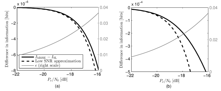
Figure 1: ${I_{\mathrm{MMSE}}}-{I_{\textrm{SL}}}$ and $\epsilon_{0}$ for (a) trinary input with high kurtosis and (b) highly skewed binary input, in the low SNR regime and under moderate ISI.

To clearly observe the behavior predicted by Theorem 1, it is crucial to use an input distribution with high skewness or high kurtosis. Using the notation of (27), we observe that the difference ${I_{\mathrm{MMSE}}}-{I_{\textrm{SL}}}$ is of the order of $s_{x}^{2}\epsilon_{0}^{3}\gamma_{1}^{3}/\beta_{0}^{6}+\kappa_{x}^{2}\epsilon_{0}^{4}\delta_{1}^{4}/\beta_{0}^{8}$. Computations reveal that for channels with moderate to high ISI, $\left|\gamma_{1}^{3}\right|/\beta_{0}^{6}$ and $\delta_{1}^{4}/\beta_{0}^{8}$ are both of the order of $0.05$ at low SNRs, and that the series approximation is valid up to $\epsilon_{0}$ values of around $0.02$. Hence, the difference term is roughly $10^{-8}s_{x}^{2}+10^{-10}\kappa_{x}^{2}$. Therefore, we must have $s_{x}^{2}$ of the order of $10$ and/or $\kappa_{x}^{2}$ of the order of $10^{3}$ for the predicted low-SNR behavior to be distinguishable from numeric errors.

We emphasize that Theorem 1 guarantees that the SLC does not hold for any input distribution with nonzero skewness or excess kurtosis, including for example BPSK input that has $s_{x}=0$ and $\kappa_{x}=-2$. However, the above analysis shows that the universal low SNR behavior (27) is masked by numerical errors when common input distributions are used, due to the facts that by symmetry they have zero skewness, and that their excess kurtosis values are of order unity. This serves to explain why similar low SNR counterexamples to the SLC were not previously reported.

III-B Medium-SNR regime — ${\mathcal{I}}<{I_{\textrm{SL}}}$

Figure 2 displays ${I_{\mathrm{MMSE}}}$, ${I_{\textrm{SL}}}$ and ${\mathcal{I}}$ computed for the input distributions and ISI channel described above. The value of ${\mathcal{I}}$ is computed by Monte-Carlo simulations as described in [7]. For each SNR, 20 simulations with input length $5\cdot 10^{8}$ were preformed. The dots on the red curve indicate the averaged result of these simulations (which is equivalent to a single simulation with input length $10^{10}$), and the error bars indicate the minimum and maximum results among the 20 simulations.

For both input distributions, ${I_{\textrm{SL}}}$ clearly exceeds ${I_{\mathrm{MMSE}}}$. In fact, further simulations indicate that in both cases ${I_{\textrm{SL}}}>{I_{\mathrm{MMSE}}}$ for the entire SNR range, leaving little room to hope that the Shamai-Laroia conjecture is valid in the high-SNR regime. For the symmetric trinary source, it is seen that ${\mathcal{I}}>{I_{\textrm{SL}}}$ for all SNRs tested. However, for the skewed binary sources, it is fairly certain that ${\mathcal{I}}<{I_{\textrm{SL}}}$ at some SNRs. This leads to the conclusion that even the modified conjecture ${\mathcal{I}}\geq{I_{\textrm{SL}}}$ does not hold in general.

The relation ${\mathcal{I}}\geq{I_{\textrm{SL}}}$ might still be true for all SNRs and ISI channels for some input distributions, such as BPSK, and might even hold for large families of input distributions, such as symmetric sources. Our simulations indicate that ${I_{\textrm{SL}}}$ is always a tight approximation for ${\mathcal{I}}$, and that it is much tighter than ${I_{\mathrm{MMSE}}}$ for sources with high skewness or excess kurtosis. Moreover, in the following section we establish that in the high-SNR regime, the inequality ${\mathcal{I}}\geq{I_{\textrm{SL}}}$ holds for any input distribution and any ISI channel.

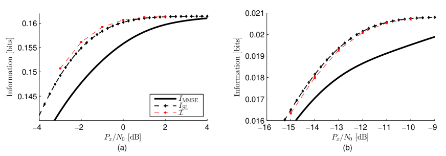
Figure 2: ${I_{\mathrm{MMSE}}}$, ${I_{\textrm{SL}}}$ and ${\mathcal{I}}$ for (a) trinary input with high kurtosis and (b) highly skewed binary input, in the medium SNR regime and under moderate ISI.

IV High SNR analysis of the Shamai-Laroia approximation

In this section we prove that the weakened Shamai-Laroia bound ${\mathcal{I}}\geq{I_{\textrm{SL}}}$ is valid for any input distribution and ISI channel, for sufficiently high SNR. The proof is carried out by bounding the exponential rates at which ${\mathcal{I}}$ and ${I_{\textrm{SL}}}$ converge to the input entropy as the input SNR grows, and showing that the former rate is strictly higher than the latter for every non-trivial ISI channel. The rate of convergence of ${\mathcal{I}}$ is lower bounded using Fano’s inequality and Forney’s analysis of the probability of error of the Maximum Likelihood sequence detector of the input to the ISI channel given its output. The rate of convergence of ${I_{\textrm{SL}}}$ is upper bounded using the I-MMSE relationship and genie-based bounds on the MMSE estimation of a single channel input from an observation contaminated by additive Gaussian noise.

For convenience, the results of this section assume the normalization $\sum_{k=0}^{L-1}h_{k}^{2}=\frac{1}{2\pi}\int_{-\pi}^{\pi}\left|H\left(\theta\right)\right|^{2}d\theta=1$. Let

$$g_{\textrm{ZF-DFE}}=\exp\left\{\frac{1}{2\pi}\int_{-\pi}^{\pi}\log\left(\left|H\left(\theta\right)\right|^{2}\right)d\theta\right\}$$ (36)

denote the gain factor of the zero-forcing DFE — It is seen that ${\mathsf{SNR}_{\textrm{DFE}}}$ behaves as $\frac{P_{x}}{N_{0}}g_{\textrm{ZF-DFE}}$ when $P_{x}/N_{0}\rightarrow\infty$. For every possible channel input $x\in\mathcal{X}$, let $p\left(x\right)$ denote its probability of occurrence and let $H\left(x_{0}\right)=-\sum_{x\in\mathcal{X}}p\left(x\right)\log p\left(x\right)$ be the input entropy. Finally, let $d_{\min}=\min_{x,x^{\prime}\in\mathcal{X}}\left|x-x^{\prime}\right|$ denote the minimal distance between different input values.

Our asymptotic bound for the achievable rate ${\mathcal{I}}$ is formally stated as follows,

Lemma 1.

For any finite entropy input distribution and any finite length ISI channel there exists a function $F\left(x\right)>0$ polynomial in $x$ and a constant $\delta_{\min}^{2}$such that,

$$H\left(x_{0}\right)-{\mathcal{I}}\leq F\left(\frac{P_{x}}{N_{0}}\right)\exp\left(-\frac{P_{x}}{2N_{0}}\left(\frac{d_{\min}}{2}\right)^{2}\delta_{\min}^{2}\right)$$ (37)

and $\delta_{\min}^{2}\geq g_{\textrm{ZF-DFE}}$, with strict inequality whenever $\left|H\left(\theta\right)\right|$ is not constant (i.e. there is non-zero ISI).

Proof:

Since $x_{-\infty}^{\infty}$ is i.i.d., $H\left(x_{0}|x_{-\infty}^{-1}\right)=H\left(x_{0}\right)$ and hence

$$H\left(x_{0}\right)-{\mathcal{I}}=H\left(x_{0}|y_{-\infty}^{\infty},x_{-\infty}^{-1}\right)\leq H\left(x_{0}|y_{-\infty}^{\infty}\right)=H\left(x_{0}|\hat{x}_{0}^{ML},y_{-\infty}^{\infty}\right)\leq H\left(x_{0}|\hat{x}_{0}^{ML}\right)$$ (38)

where $\left\{\hat{x}_{i}^{ML}\right\}_{i=-\infty}^{\infty}$ is the maximum likelihood sequence estimate of $x_{-\infty}^{\infty}$ given $y_{-\infty}^{\infty}$. By Fano’s inequality,

$$H\left(x_{0}|\hat{x}_{0}^{ML}\right) \leq H\left(x_{0},1_{\left\{x_{0}=\hat{x}_{0}^{ML}\right\}}|\hat{x}_{0}^{ML}\right)\leq H\left(1_{\left\{x_{0}=\hat{x}_{0}^{ML}\right\}}\right)+H\left(x_{0}|1_{\left\{x_{0}=\hat{x}_{0}^{ML}\right\}},\hat{x}_{0}^{ML}\right)$$ (39)

$$\leq h_{2}\left(\Pr\left(x_{0}\neq\hat{x}_{0}^{ML}\right)\right)+\Pr\left(x_{0}\neq\hat{x}_{0}^{ML}\right)\log\left|\mathcal{X}\right|$$ (40)

$$H\left(x_{0}|\hat{x}_{0}^{ML}\right)\leq h_{2}\left(\Pr\left(x_{0}\neq\hat{x}_{0}^{ML}\right)\right)+\Pr\left(x_{0}\neq\hat{x}_{0}^{ML}\right)\log\left|\mathcal{X}\right|$$ (41)

where $h_{2}\left(x\right)=-x\log x-\left(1-x\right)\log\left(1-x\right)$ is the binary entropy function and $\mathcal{X}$ is the set of possible values of $x_{0}$. By the analysis of the probability of error in maximum likelihood sequence estimation first preformed by Forney [19] and then refined in [20, 21, 22], we know that

$$\Pr\left(x_{0}\neq\hat{x}_{0}^{ML}\right)\leq K^{\prime}Q\left(\sqrt{\frac{P_{x}}{N_{0}}\left(\frac{d_{\min}}{2}\right)^{2}\delta_{\min}^{2}}\right)$$ (42)

with $K^{\prime}>0$ and $\delta_{\min}^{2}$ the minimum weighted and normalized distance between any two input sequences that first diverge at time $0$ and last diverge at some finite time $N$,

$$\delta_{\min}^{2}=\inf_{N\geq 1}\min_{\begin{array}[]{c}x_{0}^{N-1},\tilde{x}_{0}^{N-1}\mbox{ s.t. }\\ x_{0}\neq\tilde{x}_{0},x_{N-1}\neq\tilde{x}_{N-1}\end{array}}\delta^{2}\left(x_{0}^{N-1},\tilde{x}_{0}^{N-1}\right)$$ (43)

where

$$\delta^{2}\left(x_{0}^{N-1},\tilde{x}_{0}^{N-1}\right)=\sum_{k=0}^{L+N-2}\left|\sum_{l=0}^{N-1}\left(\frac{x_{l}-\tilde{x}_{l}}{d_{\min}}\right)h_{k-l}\right|^{2}$$ (44)

Substituting (42) into (40) and taking (38) into account, along with the fact that $Q\left(x\right)\leq\frac{1}{\sqrt{2\pi}}e^{-x^{2}/2}$, yields the bound (37). It remains to show that $\delta_{\min}^{2}$ can be lower bounded by $g_{\textrm{ZF-DFE}}$. By keeping only the first and last summands in (44), we have that when $L>1$, for any feasible pair of sequences $x_{0}^{N-1},\tilde{x}_{0}^{N-1}$,

$$\delta^{2}\left(x_{0}^{N-1},\tilde{x}_{0}^{N-1}\right)\geq\left|\left(\frac{x_{0}-\tilde{x}_{0}}{d_{\min}}\right)h_{0}\right|^{2}+\left|\left(\frac{x_{N-1}-\tilde{x}_{N-1}}{d_{\min}}\right)h_{L-1}\right|^{2}\geq\left|h_{0}\right|^{2}+\left|h_{L-1}\right|^{2}$$ (45)

since by assumption $x_{0}\neq\tilde{x}_{0}$ and $x_{N-1}\neq\tilde{x}_{N-1}$, and $x\neq\tilde{x}$ implies $\left|x-\tilde{x}\right|\geq d_{\min}$. Hence, $\delta_{\min}^{2}\geq\left|h_{0}\right|^{2}+\left|h_{L-1}\right|^{2}>\left|h_{0}\right|^{2}$ for $L>1$.

We may assume without loss of generality that $H\left(\theta\right)$ is minimum phase (i.e. has no zeros outside the unit circle), because it may always be brought to this form by means of a whitened matched filter. When $H\left(\theta\right)$ is minimum phase it follows that $g_{\textrm{ZF-DFE}}=\left|h_{0}\right|^{2}$, and thus we conclude that $\delta_{\min}^{2}>g_{\textrm{ZF-DFE}}$, except for the zero-ISI case $L=1$. For $L=1$, $\delta_{\min}^{2}=g_{\textrm{ZF-DFE}}=1$. ∎

Our asymptotic bound for the achievable rate for the Shamai-Laroia expression ${I_{\textrm{SL}}}$ is given as,

Lemma 2.

For any finite entropy input distribution and any finite length ISI channel there exists a function $G\left(x\right)>0$ polynomial in $x$ and constants $\varepsilon,\hat{K}>0$ such that,

$$H\left(x_{0}\right)-{I_{\textrm{SL}}}\geq G\left(\frac{P_{x}}{N_{0}}\right)\exp\left(-\frac{P_{x}}{2N_{0}}\left(\frac{d_{\min}}{2}\right)^{2}g_{\textrm{ZF-DFE}}-\hat{K}\cdot\left(\frac{P_{x}}{N_{0}}\right)^{1-\varepsilon}\right)$$ (46)

Proof:

We rewrite $I_{x}\left(\mathrm{snr}\right)$ as defined in (7) using the I-MMSE relation [16],

$$H\left(x_{0}\right)-I_{x}\left(\mathrm{snr}\right)=\frac{1}{2}\int_{\mathrm{snr}}^{\infty}\mathrm{mmse}_{\bar{x}}\left(\gamma\right)d\gamma$$ (47)

where $\bar{x}=x/\sqrt{P_{x}}$, and for any RV $z$,

$$\mathrm{mmse}_{z}\left(\gamma\right)\triangleq E\left(z-E\left[z\,|\,\sqrt{\gamma}z+n\right]\right)^{2}$$ (48)

with $n\sim\mathcal{N}\left(0,1\right)$ and independent of $z$. Let $v_{1}$ and $v_{2}$ be two possible values of $x$ such that $\left|v_{1}-v_{2}\right|=d_{\min}$, and denote their probabilities $p\left(v_{1}\right)$ and $p\left(v_{2}\right)$, respectively, assuming without loss of generality that $p\left(v_{1}\right)\leq p\left(v_{2}\right)$. Let $U$ be a random variable independent of $x$ and distributed on $\left\{0,1\right\}$ with $\Pr\left(U=1\right)=p\left(v_{1}\right)/p\left(v_{2}\right)$. Define the random variable $B=1_{\left\{x=v_{1}\right\}}+U\cdot 1_{\left\{x=v_{2}\right\}}$, so that given $B=1$, $x$ is distributed equiprobably on $\left\{v_{1},v_{2}\right\}$. Since conditioning can only decrease MMSE we have

$$\mathrm{mmse}_{\bar{x}}\left(\gamma\right)\geq\mathrm{mmse}_{\bar{x}|B}\left(\gamma\right)\geq\Pr\left(B=1\right)\mathrm{mmse}_{\bar{x}|B=1}\left(\gamma\right)$$ (49)

Now, $\Pr\left(B=1\right)=2p\left(v_{1}\right)$, and $\mathrm{mmse}_{\bar{x}|B=1}\left(\gamma\right)=\left(\frac{d_{\min}}{2}\right)^{2}\mathrm{mmse}_{b}\left(\left(\frac{d_{\min}}{2}\right)^{2}\gamma\right)$, where $b$ is equiprobably distributed on $\left\{-1,1\right\}$. The function $\mathrm{mmse}_{b}$ can be bounded as

$$\mathrm{mmse}_{b}\left(\gamma\right) = \frac{1}{\sqrt{2\pi}}\int_{-\infty}^{\infty}\left(1-\tanh\left(\sqrt{\gamma}y\right)\right)e^{-\frac{1}{2}\left(y-\sqrt{\gamma}\right)^{2}}dy$$ (50)

$$\geq \frac{1}{\sqrt{2\pi}}\int_{-\infty}^{\infty}e^{-\sqrt{\gamma}\left(y+\left|y\right|\right)}e^{-\frac{1}{2}\left(y-\sqrt{\gamma}\right)^{2}}=2Q\left(\sqrt{\gamma}\right)$$ (51)

where we have used $1-\tanh\left(x\right)\geq e^{-x-\left|x\right|}$. Using $Q\left(\sqrt{x}\right)<\frac{e^{-x/2}}{\sqrt{2\pi x}}$ we find that,

$$\int_{s}^{\infty}Q\left(\sqrt{\gamma}\right)d\gamma=\frac{\sqrt{s}e^{-s/2}}{\sqrt{2\pi}}+\left(1-s\right)Q\left(\sqrt{s}\right)\underset{s>1}{\geq}\frac{e^{-s/2}}{\sqrt{2\pi s}}$$ (52)

and so

$$\frac{1}{2}\int_{\mathrm{snr}}^{\infty}\mathrm{mmse}_{\bar{x}}\left(\gamma\right)d\gamma\geq p\left(v_{1}\right)\int_{\left(\frac{d_{\min}}{2}\right)^{2}\mathrm{snr}}^{\infty}\mathrm{mmse}_{b}\left(\gamma\right)d\gamma\geq\frac{2\sqrt{2}p\left(v_{1}\right)}{\sqrt{\pi d_{\min}^{2}\mathrm{snr}}}\exp\left(-\frac{1}{2}\mathrm{\left(\frac{d_{\min}}{2}\right)^{2}snr}\right)$$ (53)

We remark that a bound similar to (49) was developed in [23]. However, the lower bound of [23] does not take into account non-equiprobable inputs.

The last step is to upper bound ${\mathsf{SNR}_{\textrm{DFE}}}$ in terms of $g_{\textrm{ZF-DFE}}$ for large $P_{x}/N_{0}$. We have

$$\log\left(\frac{{\mathsf{SNR}_{\textrm{DFE}}}}{\frac{P_{x}}{N_{0}}g_{\textrm{ZF-DFE}}}\right)=\frac{1}{2\pi}\int_{-\pi}^{\pi}\log\left(1+\frac{N_{0}}{P_{x}\left|H\left(\theta\right)\right|^{2}}\right)d\theta$$ (54)

If $\left|H\left(\theta\right)\right|^{2}>0$ for every $\theta$, a simple bound is obtained using $\frac{1}{2\pi}\int_{-\pi}^{\pi}\log\left(f\left(\theta\right)\right)d\theta\leq\log\left(\frac{1}{2\pi}\int_{-\pi}^{\pi}f\left(\theta\right)d\theta\right)$:

$${\mathsf{SNR}_{\textrm{DFE}}}\leq\frac{P_{x}}{N_{0}}g_{\textrm{ZF-DFE}}+\frac{g_{\textrm{ZF-DFE}}}{g_{\textrm{ZF-LE}}}$$ (55)

with $g_{\textrm{ZF-LE}}=\left[\frac{1}{2\pi}\int_{-\pi}^{\pi}\frac{d\theta}{\left|H\left(\theta\right)\right|^{2}}\right]^{-1}$ being the SNR gain factor of the linear zero-forcing equalizer. However, if the channel has spectral nulls, $g_{\textrm{ZF-LE}}=0$ and the above bound is useless. In this case, let

$$\Omega=\left\{\theta\in\left[-\pi,\pi\right]\>|\>\left|H\left(\theta\right)\right|^{2}<\sqrt{N_{0}/P_{x}}\right\}$$ (56)

and for $N_{0}/P_{x}<1$, bound (54) as

$$\frac{1}{2\pi}\int_{-\pi}^{\pi}\log\left(1+\frac{N_{0}}{P_{x}\left|H\left(\theta\right)\right|^{2}}\right)d\theta\leq\frac{1}{2\pi}\int_{\Omega}\log\left(2\sqrt{\frac{N_{0}}{P_{x}}}\frac{1}{\left|H\left(\theta\right)\right|^{2}}\right)d\theta+\frac{\left|\Omega^{C}\right|}{2\pi}\log\left(1+\sqrt{\frac{N_{0}}{P_{x}}}\right)$$ (57)

The second term above is upper bounded simply as $\log\left(1+\sqrt{\frac{N_{0}}{P_{x}}}\right)$, while the first term is bounded using the Cauchy-Schwartz inequality assuming now $2\sqrt{N_{0}/P_{x}}<1$:

$$\frac{1}{2\pi}\int_{\Omega}\log\left(2\sqrt{\frac{N_{0}}{P_{x}}}\frac{1}{\left|H\left(\theta\right)\right|^{2}}\right)d\theta \leq\frac{1}{2\pi}\int_{-\pi}^{\pi}1_{\left\{\theta\in\Omega\right\}}\log\left(\frac{1}{\left|H\left(\theta\right)\right|^{2}}\right)d\theta$$ (58)

$$\leq \sqrt{\frac{\left|\Omega\right|}{2\pi}}\sqrt{\frac{1}{2\pi}\int_{-\pi}^{\pi}\log^{2}\left(\left|H\left(\theta\right)\right|^{2}\right)d\theta}$$ (59)

Since $\left|H\left(\theta\right)\right|^{2}=c\prod_{i=1}^{L-1}\left(1-\zeta_{i}\cos\left(\theta-\theta_{i}\right)\right)$ with $c>0$, $\left|\zeta_{i}\right|\leq 1$ and $\theta_{i}\in\left[-\pi,\pi\right]$ it can be shown that $\frac{1}{2\pi}\int_{-\pi}^{\pi}\log^{2}\left(\left|H\left(\theta\right)\right|^{2}\right)d\theta<c_{1}^{2}<\infty$ and $\left|\Omega\right|<2\pi c_{2}\left(N_{0}/P_{x}\right)^{\varepsilon^{\prime}}$ for some $c_{1},c_{2,},\varepsilon^{\prime}>0$. Therefore,

$${\mathsf{SNR}_{\textrm{DFE}}}\leq\frac{P_{x}}{N_{0}}g_{\textrm{ZF-DFE}}\left(1+\sqrt{\frac{N_{0}}{P_{x}}}\right)e^{c_{1}c_{2}\left(N_{0}/P_{x}\right)^{\varepsilon^{\prime}}}\leq\frac{P_{x}}{N_{0}}g_{\textrm{ZF-DFE}}+\hat{K}\left(\frac{P_{x}}{N_{0}}\right)^{1-\varepsilon}$$ (60)

for some $\varepsilon,\hat{K}>0$ and sufficiently large $P_{x}/N_{0}$.

Using (11), (47), (53) and (60) we conclude that

$$H\left(x_{0}\right)-{I_{\textrm{SL}}} \geq H\left(x_{0}\right)-I_{x}\left(\frac{P_{x}}{N_{0}}g_{\textrm{ZF-DFE}}+\hat{K}\cdot\left(\frac{P_{x}}{N_{0}}\right)^{1-\varepsilon}\right)$$

$$\geq G\left(\frac{P_{x}}{N_{0}}\right)\exp\left(-\frac{P_{x}}{2N_{0}}\left(\frac{d_{\min}}{2}\right)^{2}g_{\textrm{ZF-DFE}}-\hat{K}\cdot\left(\frac{P_{x}}{N_{0}}\right)^{1-\varepsilon}\right)$$ (61)

with $G\left(x\right)$ given by $2\sqrt{2}p\left(v_{1}\right)\left[\pi d_{\min}^{2}\left(g_{\textrm{ZF-DFE}}x+\hat{K}x^{1-\varepsilon}\right)\right]^{-1/2}$ . ∎

Using the above results, we are able to state our desired conclusion,

Theorem 2.

For any finite entropy input distribution and any finite length ISI channel, ${\mathcal{I}}\geq{I_{\textrm{SL}}}$ for sufficiently high SNR.

Proof:

Immediate from Lemmas 1 and 2. ∎

V Information-Estimation-based bounds for ${I_{\mathrm{MMSE}}}$

Having shown that ${I_{\textrm{SL}}}$ is not always a lower bound on ${I_{\mathrm{MMSE}}}$ and that sometimes it is not even a lower bound for ${\mathcal{I}}$, in this section we establish new lower bounds for ${I_{\mathrm{MMSE}}}$ and hence for ${\mathcal{I}}$. The bounds are based on a simple genie-based bound for the MMSE in estimating a linear combination of i.i.d. variables from their Gaussian noise corrupted version, that are related to ${I_{\mathrm{MMSE}}}$ via the Guo-Shamai-Verdú theorem. A general bound with two scalar parameters is derived. These parameters may be either easily optimized numerically, or fixed in order to yield a simpler expression, which is optimal for low SNR’s and nearly as tight in the high SNR regime. The bounds are evaluated and compared with recently proposed lower bounds for ${I_{\mathrm{MMSE}}}$ where the input is binary. They are found to be quite tight at low SNR’s, reasonable at medium SNR’s and loose for high SNR’s.

V-A A general MMSE bound

Consider the random variable

$$X=\sum_{k\in{\mathcal{K}}}a_{k}x_{k}$$ (62)

where $x_{k}$ are i.i.d. RVs with $Ex^{2}=1$, ${\mathcal{K}}\subseteq\mathbb{N}$ and the coefficients $\left\{a_{k}\right\}_{k\in{\mathcal{K}}}$ satisfy $\sum_{k\in{\mathcal{K}}}a_{k}^{2}=1$. Let $Y=\sqrt{\gamma}X+N$ with $N$ a standard Gaussian variable independent of $X$, so that by (48),

$$\textrm{mmse}_{X}(\gamma)=E\left(X-E[X\,|\,Y]\right)^{2}$$ (63)

Let $\left\{{\mathcal{P}}_{m}\right\}_{m\in{\mathcal{M}}}$ be a partition of ${\mathcal{K}}$ and define for every $m\in{\mathcal{M}}$,

$$b_{m}^{2} = \sum_{k\in{\mathcal{P}}_{m}}a_{k}^{2}$$ (64)

$$X_{m} =\frac{1}{b_{m}} \sum_{k\in{\mathcal{P}}_{m}}a_{k}x_{k}$$ (65)

and

$$Y_{m}=\sqrt{\gamma}X_{m}+N_{m}$$ (66)

where $\left\{N_{m}\right\}_{m\in{\mathcal{M}}}$ are independent with $N_{m}\sim\mathcal{N}(0,\sigma_{m}^{2})$ and satisfy $\sum_{m\in{\mathcal{M}}}b_{m}^{2}\sigma_{m}^{2}=1$.

Lemma 3.

Under the above definitions,

$$\textrm{mmse}_{X}(\gamma)\geq\sum_{m\in{\mathcal{M}}}b_{m}^{2}\textrm{mmse}_{X_{m}}(\frac{\gamma}{\sigma_{m}^{2}})$$ (67)

Proof:

Note that we may write $Y=\sum_{m\in{\mathcal{M}}}b_{m}Y_{m}$. Since conditioning decreases MMSE,

$$\textrm{mmse}_{X}(\gamma)\geq E\left(X-E\left[X|\left\{Y_{m}\right\}_{m\in{\mathcal{M}}}\right]\right)^{2}$$ (68)

For every $m\neq m^{\prime}$, $X_{m}$ is independent of $X_{m^{\prime}}$ and $Y_{m^{\prime}}$. Writing $X=\sum_{m\in{\mathcal{M}}}b_{m}X_{m}$, we find that

$$E\left(X-E\left[X|\left\{Y_{m}\right\}_{m\in{\mathcal{M}}}\right]\right)^{2}=\sum_{m\in{\mathcal{M}}}b_{m}^{2}E\left(X_{m}-E\left[X_{m}|Y_{m}\right]\right)^{2}=\sum_{m\in{\mathcal{M}}}b_{m}^{2}\textrm{mmse}_{X_{m}}(\frac{\gamma}{\sigma_{m}^{2}})$$ (69)

∎

Specializing to $\sigma_{m}^{2}=1/\sum_{k\in{\mathcal{K}}}a_{k}^{2}$ for any $m\in{\mathcal{M}}$ yields the bound,

$$\textrm{mmse}_{X}(\gamma)\geq\sum_{m=1}^{M}b_{m}^{2}\textrm{mmse}_{X_{m}}\left(\gamma\right)$$ (70)

Specializing further to ${\mathcal{P}}_{k}=\left\{k\right\}$ for any $k\in{\mathcal{K}}$ (${\mathcal{M}}={\mathcal{K}}$) yields the very simple bound

$$\textrm{mmse}_{X}(\gamma)\geq\textrm{mmse}_{x}\left(\gamma\right)$$ (71)

Another interesting choice is $\sigma_{m^{\prime}}^{2}=1/b_{m^{\prime}}^{2}$ for some $m^{\prime}$ and $\sigma_{m}^{2}=0$ for all $m\neq m^{\prime}$. In this case,

$$\textrm{mmse}_{X}(\gamma)\geq b_{m^{\prime}}^{2}\textrm{mmse}_{X_{m}}\left(b_{m^{\prime}}^{2}\gamma\right)$$ (72)

Applying (70) to $\textrm{mmse}_{X_{m}}\left(\cdot\right)$ in (72) yields the simpler bound,

$$\textrm{mmse}_{X}(\gamma)\geq b_{m^{\prime}}^{2}\textrm{mmse}_{x}\left(b_{m^{\prime}}^{2}\gamma\right)$$ (73)

Note that the smaller $b_{m^{\prime}}$ is, the tighter the bound in high SNR’s, while the opposite is true for low SNR’s.

V-B Information-Estimation application

In this subsection we will rely on the definitions of $\mu_{0},\mu_{1}$ and $\beta_{0},\beta_{1}$ as given in (13) and (16), respectively. We also define

$$S\triangleq\frac{P_{x}}{E{\hat{m}}^{2}}$$ (74)

with $P_{x}$ the input power and $\hat{m}$ the Gaussian noise component resulting from the application of the unbiased MMSE-DFE on the channel output. Explicit expressions for $S,\beta_{1}$ and $\beta_{0}$ in terms of the ISI channel transfer function $H\left(\theta\right)$ are given in Appendix A, in (94), (95) and (96), respectively. Under this notation, are bound is given in the following,

Theorem 3.

For any input distribution and any ISI channel,

$${I_{\mathrm{MMSE}}}\geq I_{\mathrm{IE}}\left(\gamma_{1},\gamma_{2}\right)\triangleq I_{x}(\beta_{0}^{2}\gamma_{1})-I_{x}\left(\gamma_{1}\right)+I_{x}\left(\gamma_{2}\right)-\frac{1}{2}\log\left(1+\beta_{1}^{2}\gamma_{2}\right)$$ (75)

For any $0\leq\gamma_{1}\leq\gamma_{2}\leq S$.

Proof:

As is the proof of Theorem 1 we rewrite ${I_{\mathrm{MMSE}}}$ as

$${I_{\mathrm{MMSE}}}=I\left(\mu_{0}\>;\>\mu_{0}+\hat{m}\right)-I\left(\mu_{1}\>;\>\mu_{1}+\hat{m}\right)$$ (76)

We use the Guo-Shamai-Vedú theorem [16] to write

$$2I\left(\mu_{0}\>;\>\mu_{0}+\hat{m}\right)=\int_{0}^{\beta_{0}^{2}\gamma_{1}}+\int_{\beta_{0}^{2}\gamma_{1}}^{\beta_{0}^{2}\gamma_{2}}+\int_{\beta_{0}^{2}\gamma_{2}}^{\beta_{0}^{2}S}\textrm{mmse}_{\bar{\mu}_{0}}\left(\gamma\right)d\gamma$$ (77)

$$2I\left(\mu_{1}\>;\>\mu_{1}+\hat{m}\right)=\int_{0}^{\beta_{1}^{2}\gamma_{2}}+\int_{\beta_{1}^{2}\gamma_{2}}^{\beta_{1}^{2}S}\textrm{mmse}_{\bar{\mu}_{1}}\left(\gamma\right)d\gamma$$ (78)

where $\bar{\mu}_{i}=\mu_{i}/\beta_{i}=\sum_{k\geq i}\alpha_{k}x_{k}/\beta_{i}$ is scaled to unit power. Since $\bar{\mu}_{0}$ is a unit power sum of scaled i.i.d. random variables, Lemma 3 and the bounds derived from it apply. For $0\leq\gamma\leq\beta_{0}^{2}\gamma_{1}$, we apply the bound (71) to obtain,

$$\int_{0}^{\beta_{0}^{2}\gamma_{1}}\textrm{mmse}_{\bar{\mu}_{0}}\left(\gamma\right)d\gamma\geq\int_{0}^{\beta_{0}^{2}\gamma_{1}}\textrm{mmse}_{\bar{x}}\left(\gamma\right)d\gamma=2I_{x}\left(\beta_{0}^{2}\gamma_{1}\right)$$ (79)

where $\bar{x}=x/\sqrt{P_{x}}$.

For $\beta_{0}^{2}\gamma_{1}\leq\gamma\leq\beta_{0}^{2}\gamma_{2}$, we apply (73) with only $x_{0}$ is the chosen subset, i.e. ${\mathcal{P}}_{m^{\prime}}=\left\{0\right\}$, yielding

$$\int_{\beta_{0}^{2}\gamma_{1}}^{\beta_{0}^{2}\gamma_{2}}\textrm{mmse}_{\bar{\mu}_{0}}\left(\gamma\right)d\gamma\geq\int_{\beta_{0}^{2}\gamma_{1}}^{\beta_{0}^{2}\gamma_{2}}\frac{1}{\beta_{0}^{2}}\textrm{mmse}_{\bar{x}}\left(\frac{1}{\beta_{0}^{2}}\gamma\right)d\gamma=2I_{x}\left(\gamma_{2}\right)-2I_{x}\left(\gamma_{1}\right)$$ (80)

since $b_{m^{\prime}}^{2}=\alpha_{0}^{2}/\beta_{0}^{2}=1/\beta_{0}^{2}$.

For $\beta_{0}^{2}\gamma_{2}\leq\gamma\leq\beta_{0}^{2}S$, we apply (72) with the chosen subsets including all indices but $0$, i.e. ${\mathcal{P}}={\mathcal{K}}\setminus\left\{0\right\}$, yielding

$$\int_{\beta_{0}^{2}\gamma_{2}}^{\beta_{0}^{2}S}\textrm{mmse}_{\bar{\mu}_{0}}\left(\gamma\right)d\gamma\geq\int_{\beta_{0}^{2}S\gamma_{2}}^{\beta_{0}^{2}S}\frac{\beta_{1}^{2}}{\beta_{0}^{2}}\textrm{mmse}_{\bar{\mu}_{1}}\left(\frac{\beta_{1}^{2}}{\beta_{0}^{2}}\gamma\right)d\gamma=\int_{\beta_{1}^{2}\gamma_{2}}^{\beta_{1}^{2}S}\textrm{mmse}_{\bar{\mu}_{1}}\left(\gamma\right)d\gamma$$ (81)

Finally, applying the Gaussian upper bound $\textrm{mmse}_{\bar{\mu}_{1}}\left(\gamma\right)\leq 1/\left(1+\gamma\right)$ we have

$$\int_{0}^{\beta_{1}^{2}\gamma_{2}}\textrm{mmse}_{\bar{\mu}_{1}}\left(\gamma\right)d\gamma\leq\log\left(1+\beta_{1}^{2}\gamma_{2}\right)$$ (82)

Substituting (79), (80) and (81) to (77), (82) to (78), and (77) and (78) into (76) yields the desired result. ∎

Choosing $\gamma_{1}=\gamma_{2}=S$ yields the following simple bound

$${I_{\mathrm{MMSE}}}\geq I_{\mathrm{IE},simple}\triangleq I_{x}\left(\beta_{0}^{2}S\right)-\frac{1}{2}\log\left(1+\beta_{1}^{2}S\right)$$ (83)

Note that $\frac{1}{2}\log\left(1+\gamma\right)=I_{g}\left(\gamma\right)$ is the Gaussian mutual information function. Also note that the bound holds with equality for Gaussian inputs, i.e. ${\mathcal{I}}_{g}=I_{g}\left(\beta_{0}^{2}S\right)-I_{g}\left(\beta_{1}^{2}S\right)$, where ${\mathcal{I}}_{g}$ is the i.i.d. channel capacity given in (3). The bound $I_{\mathrm{IE},simple}$ simple is guaranteed to be tight for sufficiently low SNR’s, since $I_{x}\left(\gamma\right)\approx I_{g}\left(\gamma\right)\approx\gamma/2$ as $\gamma$ tends to zero. It also guaranteed to be tight for sufficiently high SNR’s, since $\beta_{0}^{2}S\to\infty$ and $\beta_{1}^{2}S\to 0$ and $P_{x}/N_{0}\to\infty$, ensuring that $I_{\mathrm{IE},simple}$ converges to the input entropy.

The above discussion leads us to conjecture that

$$I_{\mathrm{IE},conj}\triangleq I_{x}\left(\beta_{0}^{2}S\right)-I_{x}\left(\beta_{1}^{2}S\right)$$ (84)

is also a lower bound for ${I_{\mathrm{MMSE}}}$. This is equivalent to conjecturing that the bound $I\left(\mu_{0}\>;\>\mu_{0}+\hat{m}\right)\geq I_{x}\left(\beta_{0}^{2}S\right)$ is always looser than the bound $I\left(\mu_{1}\>;\>\mu_{1}+\hat{m}\right)\geq I_{x}\left(\beta_{1}^{2}S\right)$ , i.e. that

$$I\left(\mu_{0}\>;\>\mu_{0}+\hat{m}\right)-I_{x}\left(\beta_{0}^{2}S\right)\geq I\left(\mu_{1}\>;\>\mu_{1}+\hat{m}\right)-I_{x}\left(\beta_{1}^{2}S\right)$$

Attempts to prove this conjectured bound were so far unsuccessful. In all simulations preformed, $I_{\mathrm{IE},conj}$ never exceeded ${I_{\mathrm{MMSE}}}$, supporting this conjecture. However, for common input distributions such as BPSK, $I_{\mathrm{IE},conj}$ was seen to offer very little improvement over $I_{\mathrm{IE},simple}$, even for channels with severe ISI. This is due to the fact that generally, $E\mu_{1}^{2}$ is of the order of $E{\hat{m}}^{2}$ or smaller, and therefore the mutual information $I\left(\mu_{1}\>;\>\mu_{1}+\hat{m}\right)$ is very well approximated by the Gaussian upper bound. In the simulations described in the following subsection, the difference between $I_{\mathrm{IE},conj}$ and $I_{\mathrm{IE},simple}$ was not noticeable and therefore only $I_{\mathrm{IE},simple}$ was plotted.

Let

$${I_{\mathrm{MMSE}}}\geq I_{\mathrm{IE},opt}\triangleq\max_{0\leq\gamma_{1}\leq\gamma_{2}\leq S}I_{\mathrm{IE}}\left(\gamma_{1},\gamma_{2}\right)$$ (85)

be the optimal lower bound, and let $\gamma_{1}^{*}$ and $\gamma_{2}^{*}$ be its optimizers. The values $\gamma_{1}^{*}$, $\gamma_{2}^{*}$ can be easily determined using the following procedure. If $\beta_{0}^{2}\textrm{mmse}_{\bar{x}}\left(\beta_{0}^{2}S\right)\geq\textrm{mmse}_{\bar{x}}\left(S\right)$, then $\gamma_{1}^{*}=\gamma_{2}^{*}=S$ and $I_{\mathrm{IE},opt}=I_{\mathrm{IE},simple}$. Otherwise, $\gamma_{1}^{*}$ satisfies

$$\beta_{0}^{2}\textrm{mmse}_{\bar{x}}\left(\beta_{0}^{2}\gamma_{1}^{*}\right)=\textrm{mmse}_{\bar{x}}\left(\gamma_{1}^{*}\right)$$ (86)

Next, if $\textrm{mmse}_{\bar{x}}\left(S\right)\geq\beta_{1}^{2}/\left(1+\beta_{1}^{2}S\right)$, then $\gamma_{2}^{*}=S$. Otherwise, $\gamma_{2}^{*}$ satisfies

$$\textrm{mmse}_{\bar{x}}\left(\gamma_{2}^{*}\right)=\frac{\beta_{1}^{2}}{1+\beta_{1}^{2}\gamma_{2}^{*}}$$ (87)

We conclude by noting that the bound (75) can be further generalized using Lemma 3 by using other partitions of the ISI taps and adding further degrees of freedom to the optimization. However, numerical experimentation indicates that such generalizations offer very little improvement in tightness.

V-C Evaluation of the bounds

Figure 3 plots ${I_{\mathrm{MMSE}}}$, ${I_{\textrm{SL}}}$, the Shamai-Ozarow-Wyner bound ${I_{\textrm{SOW}}}$ (6) and the bounds $I_{\mathrm{IE},opt}$ and $I_{\mathrm{IE},simple}$, for BPSK input the most severe example ISI channel that appeared in [13],

$$h=\left[0.19,\,0.35,\,0.46,\,0.5,\,0.46,\,0.35,\,0.19\right]$$ (88)

The lower bounds $C_{L1,0}$ and $C_{L1,3}$ proposed in [13] are also plotted. ${I_{\mathrm{MMSE}}}$ has been approximated using the procedure described in Section III.

It is seen that the proposed bounds $I_{\mathrm{IE},opt}$ and $I_{\mathrm{IE},simple}$ are identical and tight in the low SNR region. For medium to high SNR’s, $I_{\mathrm{IE},opt}$ improves on $I_{\mathrm{IE},simple}$, but both bounds are not very tight. Additionally, ${I_{\textrm{SOW}}}$ is very loose in this example, reflecting the poor performance of decision feedback zero-forcing equalization in severe ISI conditions. In comparison to the bounds from [13], $I_{\mathrm{IE},opt}$ and $I_{\mathrm{IE},simple}$ are tighter than the simple single-letter bound $C_{L1,0}$ in the low to medium SNR region, but are less tight for higher SNR’s. The tightened 3-letter bound $C_{L1,3}$ is tighter than our proposed bound for all SNR’s.

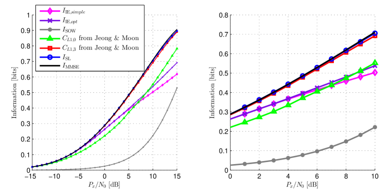
Figure 3: Comparison of bounds for ${I_{\mathrm{MMSE}}}$ for BPSK input and ISI channel (88)

As reported in [13], the bounds reported there become looser when there is no small set of dominant coefficients in the residual ISI sequence $\alpha_{1}^{\infty}$, as often happens in highly scattered multipath channels. In order to simulate such channel, the impulse response (88) was spaced by adding 3 and 5 null taps around the main tap, yielding,

$$\tilde{h}=[0.19,\,0.35,\,0.46,\,\underset{3}{\underbrace{0\cdots 0}},\,0.5,\,\underset{5}{\underbrace{0\cdots 0}},\,0.46,\,0.35,\,0.19]$$ (89)

The experiment described above was repeated with the modified ISI channel (89), and the results are shown in Figure 4. It is seen that here the bounds of [13] are considerably looser, while our proposed bounds retain their tightness. The bound in [13] may be tightened by increasing the parameter $M$ beyond 3, but at the cost of an exponentially increasing computational load and loss of analytic tractability. It is interesting to note that the spacing of the ISI channel has actually reduced the severity of the ISI — this is evident from the higher information rates attained, as well as from the improvement in tightness of the Shamai-Ozarow-Wyner bound. In fact, in this experiment ${I_{\textrm{SOW}}}$ proved to be the tightest bound in high SNR’s.

As a last point of comparison we remark that our bounds apply to any input distribution, while the bounds of [13] are developed only for symmetric binary input.

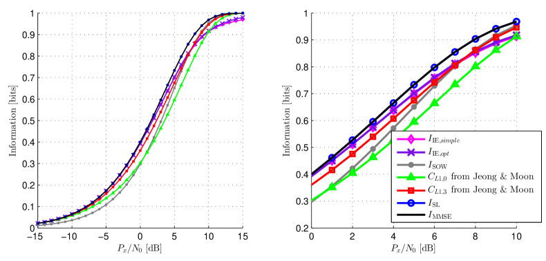
Figure 4: Comparison of bounds for ${I_{\mathrm{MMSE}}}$ for BPSK input and ISI channel (89)

VI Conclusion

This paper addressed the long-standing Shamai-Laroia conjecture from several directions. First, the original conjecture was shown analytically not to hold. Next, a natrual relaxation of the conjecture was considered, in which ${I_{\textrm{SL}}}$ is proposed as a lower bound for ${\mathcal{I}}$, the single-carrier achievable rate. It was shown by means of Monte-Carlo simulation that this weakened conjecture does not hold as well, by means of a counterexample based on a highly skewed binary input. A positive result on the relaxed conjecture ${\mathcal{I}}\geq{I_{\textrm{SL}}}$ is then presented, showing that it holds in the high SNR regime. Finally, alternative bounds for the achievable rate are proven. While not as tight as ${I_{\textrm{SL}}}$, these bounds have expressions nearly as simple.

Enabling all of our results are recently discovered properties of the mutual information in the scalar additive Gaussian channel with arbitrarily distributed inputs. Namely, the low SNR power series of [17] and the Guo-Shamai-Verdú Information-Estimation relation [16] find useful application in this work.

Both the negative and positive results in this paper are of practical relevance, as ${I_{\textrm{SL}}}$ is an often used approximation for the achievable rate in the ISI channel. On the one hand, we disprove the conjecture that ${I_{\textrm{SL}}}$ is a lower bound to the achievable rate, invoking caution when it is used as such. On the other hand, our high-SNR proof that ${\mathcal{I}}\geq{I_{\textrm{SL}}}$ helps to theoretically establish ${I_{\textrm{SL}}}$ as a good approximation.

A remaining open question is whether the inequality ${\mathcal{I}}\geq{I_{\textrm{SL}}}$ is true for all SNR’s for commonly used input distributions such as PSK or QAM. While numeric experimentation supports this refined conjecture, no theoretical proof is known. This question is of particular interest in the context of comparison between the achievable rates of OFDM and single-carrier modulation in the ISI channel, where a fixed i.i.d. input distribution is assumed. In this setting, ${I_{\textrm{SL}}}$ can be shown to essentially act as an upper bound for the OFDM achievable rate [24]. Thus, proving that ${\mathcal{I}}\geq{I_{\textrm{SL}}}$ for a given input distribution is tantamount to showing that the single-carrier achievable rate is superior to that of OFDM, regardless of the specific ISI channel, as long as that distribution is used.

Appendix A Noise and interference variance in the MMSE-DFE

In this section we derive closed form expressions for the quantities $\beta_{0},\beta_{1},\epsilon_{0}$ and $S$ defined in equations (16), (17) and (74), respectively. The expressions are given in terms of the output SNRs of the linear and decision-feedback MMSE equalizers, which in turn admit simple expressions in terms of the ISI channel transfer function $H\left(\theta\right)=\sum_{n}h_{n}e^{-jn\theta}$.

As in (10), the output of the unbiased MMSE at samples 0 given by

$$z_{0}=x_{0}+\sum_{k\geq 1}\hat{\alpha}_{k}x_{k}+\hat{m}$$

where $x_{-\infty}^{\infty}$ is the channel input sequence, ${\hat{\alpha}}_{1}^{\infty}$ are the residual ISI coefficients and $\hat{m}$ is an independent Gaussian noise component. The values of ${\hat{\alpha}}_{1}^{\infty}$ and $E{\hat{m}}^{2}$ maximize

$$\frac{P_{x}}{E\left(\sum_{k\geq 1}\hat{\alpha}_{k}x_{k}+\hat{m}\right)^{2}}={\mathsf{SNR}_{\textrm{DFE-U}}}={\mathsf{SNR}_{\textrm{DFE}}}-1$$ (90)

where

$${\mathsf{SNR}_{\textrm{LE}}}=\left[\frac{1}{2\pi}{\displaystyle\intop_{-\pi}^{\pi}\frac{d\theta}{1+\frac{P_{x}}{N_{0}}\left|H(\theta)\right|^{2}}}\right]^{-1}$$ (91)

$${\mathsf{SNR}_{\textrm{DFE}}}=\exp\left\{\frac{1}{2\pi}{\displaystyle\intop_{-\pi}^{\pi}\log\left[1+\frac{P_{x}}{N_{0}}\left|H(\theta)\right|^{2}\right]d\theta}\right\}$$ (92)

stand for SNR of the (biased) linear and decision-feedback equalizers, respectively

An explicit expression for the output of the biased MMSE-DFE is given in equation (50) of [12], from which it can be read that the PSD of the Gaussian noise component is given by

$$\left(\frac{P_{x}/N_{0}}{{\mathsf{SNR}_{\textrm{DFE}}}}\right)^{2}\frac{{\mathsf{SNR}_{\textrm{DFE}}}N_{0}\left|H\left(\theta\right)\right|^{2}}{1+\frac{P_{x}}{N_{0}}\left|H\left(\theta\right)\right|^{2}}=\left(\frac{P_{x}}{{\mathsf{SNR}_{\textrm{DFE}}}}\right)\frac{\frac{P_{x}}{N_{0}}\left|H\left(\theta\right)\right|^{2}}{1+\frac{P_{x}}{N_{0}}\left|H\left(\theta\right)\right|^{2}}$$

It is also shown in [12] that the unbiased MMSE-DFE is obtained by scaling the output of the MMSE-DFE by a factor of ${\mathsf{SNR}_{\textrm{DFE}}}/\left({\mathsf{SNR}_{\textrm{DFE}}}-1\right)$. Combining these expressions it seen that,

$$E{\hat{m}}^{2} = P_{x}\frac{{\mathsf{SNR}_{\textrm{DFE}}}}{\left({\mathsf{SNR}_{\textrm{DFE}}}-1\right)^{2}}\frac{1}{2\pi}{\displaystyle\intop_{-\pi}^{\pi}\left[1-\frac{1}{1+\frac{P_{x}}{N_{0}}\left|H\left(\theta\right)\right|^{2}}\right]}d\theta$$ (93)

$$=P_{x} \frac{{\mathsf{SNR}_{\textrm{DFE}}}}{\left({\mathsf{SNR}_{\textrm{DFE}}}-1\right)^{2}}\frac{{\mathsf{SNR}_{\textrm{LE}}}-1}{{\mathsf{SNR}_{\textrm{LE}}}}$$

and

$$S=\frac{P_{x}}{E{\hat{m}}^{2}}=\frac{\left({\mathsf{SNR}_{\textrm{DFE}}}-1\right)^{2}}{{\mathsf{SNR}_{\textrm{DFE}}}}\frac{{\mathsf{SNR}_{\textrm{LE}}}}{{\mathsf{SNR}_{\textrm{LE}}}-1}$$ (94)

Noticing that $E\left(\sum_{k\geq 1}\hat{\alpha}_{k}x_{k}+\hat{m}\right)^{2}=\beta_{1}^{2}P_{x}+E{\hat{m}}^{2}$ and plugging (93) into (90), we find that

$$\beta_{1}^{2}=\frac{1}{{\mathsf{SNR}_{\textrm{DFE}}}-1}-\frac{E{\hat{m}}^{2}}{P_{x}}=\frac{{\mathsf{SNR}_{\textrm{DFE}}}/{\mathsf{SNR}_{\textrm{LE}}}-1}{\left({\mathsf{SNR}_{\textrm{DFE}}}-1\right)^{2}}$$ (95)

and hence

$$\beta_{0}^{2}=1+\beta_{1}^{2}=\frac{{\mathsf{SNR}_{\textrm{DFE}}}}{{\mathsf{SNR}_{\textrm{DFE}}}-1}\left[1-\left({\mathsf{SNR}_{\textrm{LE}}}\right)^{-1}\frac{{\mathsf{SNR}_{\textrm{LE}}}-1}{{\mathsf{SNR}_{\textrm{DFE}}}-1}\right]$$ (96)

Combining the above results we find that

$$\epsilon_{1}=\frac{P_{x}\beta_{1}^{2}}{E{\hat{m}}^{2}}=\frac{1-{\mathsf{SNR}_{\textrm{LE}}}/{\mathsf{SNR}_{\textrm{DFE}}}}{{\mathsf{SNR}_{\textrm{LE}}}-1}$$ (97)

and

$$\epsilon_{0}=\frac{P_{x}\beta_{0}^{2}}{E{\hat{m}}^{2}}={\mathsf{SNR}_{\textrm{LE}}}\frac{{\mathsf{SNR}_{\textrm{DFE}}}-1}{{\mathsf{SNR}_{\textrm{LE}}}-1}-1$$ (98)

References

• [1] R.M. Gray. Entropy and information theory. Springer Verlag, 2010.
• [2] Thomas M Cover and Joy A Thomas. Elements of information theory. John Wiley & Sons, 2012.
• [3] H.D. Pfister, J.B. Soriaga, and P.H. Siegel. On the achievable information rates of finite state ISI channels. In Global Telecommunications Conference, 2001. GLOBECOM’01. IEEE, volume 5, pages 2992–2996. IEEE, 2001.
• [4] A. Radosevic, D. Fertonani, T.M. Duman, J.G. Proakis, and M. Stojanovic. Bounds on the information rate for sparse channels with long memory and iud inputs. Communications, IEEE Transactions on, 59(12):3343–3352, 2011.
• [5] F. Rusek and D. Fertonani. Lower bounds on the information rate of intersymbol interference channels based on the Ungerboeck observation model. In Information Theory, 2009. ISIT 2009. IEEE International Symposium on, pages 1649–1653. IEEE, 2009.
• [6] P. Sadeghi, P.O. Vontobel, and R. Shams. Optimization of information rate upper and lower bounds for channels with memory. Information Theory, IEEE Transactions on, 55(2):663–688, 2009.
• [7] Dieter M Arnold, H-A Loeliger, Pascal O Vontobel, Aleksandar Kavcic, and Wei Zeng. Simulation-based computation of information rates for channels with memory. Information Theory, IEEE Transactions on, 52(8):3498–3508, 2006.
• [8] D. Arnold and H.A. Loeliger. On the information rate of binary-input channels with memory. In Communications, 2001. ICC 2001. IEEE International Conference on, volume 9, pages 2692–2695. IEEE, 2001.
• [9] S. Shamai and R. Laroia. The intersymbol interference channel: Lower bounds on capacity and channel precoding loss. Information Theory, IEEE Transactions on, 42(5):1388–1404, 1996.
• [10] Edward A Lee, David G Messerschmitt, et al. Digital communications. Springer, 2004.
• [11] S. Shamai, L.H. Ozarow, and A.D. Wyner. Information rates for a discrete-time Gaussian channel with intersymbol interference and stationary inputs. Information Theory, IEEE Transactions on, 37(6):1527–1539, 1991.
• [12] J.M. Cioffi, G.P. Dudevoir, M. Vedat Eyuboglu, and G.D. Forney Jr. MMSE decision-feedback equalizers and coding I: Equalization results. Communications, IEEE Transactions on, 43(10):2582–2594, 1995.
• [13] S. Jeong and J. Moon. Easily computed lower bounds on the information rate of intersymbol interference channels. Information Theory, IEEE Transactions on, 58(2):864–877, 2012.
• [14] Aleksandar Kavcic, Xiao Ma, and Michael Mitzenmacher. Binary intersymbol interference channels: Gallager codes, density evolution, and code performance bounds. Information Theory, IEEE Transactions on, 49(7):1636–1652, 2003.
• [15] E. Abbe and L. Zheng. A coordinate system for Gaussian Networks. Information Theory, IEEE Transactions on, 58(2):721–733, 2012.
• [16] D. Guo, S. Shamai, and S. Verdú. Mutual information and minimum mean-square error in gaussian channels. Information Theory, IEEE Transactions on, 51(4):1261–1282, 2005.
• [17] Dongning Guo, Yihong Wu, Shlomo Shamai, and Sergio Verdú. Estimation in gaussian noise: Properties of the minimum mean-square error. Information Theory, IEEE Transactions on, 57(4):2371–2385, 2011.
• [18] J.G. Proakis. Digital communications, volume 1221. McGraw-hill, 1987.
• [19] G. Forney Jr. Maximum-likelihood sequence estimation of digital sequences in the presence of intersymbol interference. Information Theory, IEEE Transactions on, 18(3):363–378, 1972.
• [20] G. Foschini. Performance bound for maximum-likelihood reception of digital data. Information Theory, IEEE Transactions on, 21(1):47–50, 1975.
• [21] AD Wyner. Upper bound on error probability for detection with unbounded intersymbol interference. Bell System Technical Journal, 1975.
• [22] S. Verdú. Maximum likelihood sequence detection for intersymbol interference channels: A new upper bound on error probability. Information Theory, IEEE Transactions on, 33(1):62–68, 1987.
• [23] A. Lozano, A.M. Tulino, and S. Verdú. Optimum power allocation for parallel gaussian channels with arbitrary input distributions. Information Theory, IEEE Transactions on, 52(7):3033–3051, 2006.
• [24] Yair Carmon, Shlomo Shamai, and Tsachy Weissman. Comparison of the achievable rates in OFDM and single carrier modulation with i.i.d. inputs. arXiv preprint arXiv:1306.5781, 2013.