Quantum tomography meets dynamical systems and bifurcations theory

Abstract

A powerful tool for studying geometrical problems in Hilbert space is developed. In particular, we study the quantum pure state tomography problem in finite dimensions from the point of view of dynamical systems and bifurcations theory. First, we introduce a generalization of the Hellinger metric for probability distributions which allows us to find a geometrical interpretation of the quantum state tomography problem. Thereafter, we prove that every solution to the state tomography problem is an attractive fixed point of the so–called physical imposition operator. Additionally, we demonstrate that multiple states corresponding to the same experimental data are associated to bifurcations of this operator. Such a kind of bifurcations only occurs when informationally incomplete set of observables are considered. Finally, we prove that the physical imposition operator has a non–contractive Lipschitz constant 2 for the Bures metric. This value of the Lipschitz constant manifests the existence of the quantum tomography problem for pure states.

Keywords: Quantum state tomography, Dynamical systems theory, Bifurcations theory.

I Introduction

In earlier times of quantum mechanics W. Pauli posed an intriguing comment in a footnote Pauli . He mentioned that the problem to univocally determine the wave function of a particle from the knowledge of position and momentum distributions was not fully explored. This question, known as Pauli problem, is the origin of the quantum state reconstruction problem currently denominated quantum state tomography. The importance of quantum tomography increased in the last years due to its important role in the so called quantum technologies (quantum teleportation, quantum computing, quantum metrology, etc). Concerning finite dimensional Hilbert spaces some progresses have been found. For example, the statistics obtained from measuring three probability distributions associated to the spin observables $S_{x},S_{y}$ and $S_{z}$ is enough to reconstruct almost all quantum states, up to a null measure set in Hilbert space Weigert2 . Furthermore, Moroz and Perelomov have proven that the statistics collected from any three observables is not enough to reconstruct any quantum state in dimensions $d\geq 9$ Moroz . More recently, from considering compressed sensing it has been proven that rank $r$ observables can be reconstructed from $O(rd\log^{2}d)$ measurements Gross . Also, an informationally complete set of observables for pure states has been found, where the number of rank–one projective measurements is linear with the dimension Goyeneche4 . On the other hand, the Pauli problem also exists in infinite dimensional Hilbert spaces Corbett ; Stulpe ; Krahmer ; Corbett2 where it is close related to radar signals theory Jaming ; Orlowski .

In this work, we prove that dynamical systems and bifurcations theory are suitable tools to have a deep understanding of several geometrical problems existing in Hilbert spaces such as quantum state reconstruction problem, mutually unbiased bases, symmetric informationally complete POVM and real and complex Hadamard matrices. Here, our explanations and proves are mainly focused on the quantum state reconstruction problem. Despite this, the extension to any of the problems mentioned above is straightforward. In Section II we present an introduction to the quantum state reconstruction problem. The aim of this section is to present the minimum of contents required to understand this work. Expert readers may skip this section. In Section III we define some metrics which are required to prove the convergence of the sequences involved in our method. Here, we introduce the novel concept of distributional metric which is a generalization of the well known Hellinger metric. This new metric allows us to compare the distance between probability distributions contained in quantum states. Additionally, from a simple geometrical argument involving this metric we intuitively explain why the Pauli problem exists. In Section IV we define the physical imposition operator and we prove that every solution to the quantum state reconstruction problem is an attractive fixed point of this operator. In Section V we explain the connection between quantum state tomography and bifurcation theory. Finally, in Section VI we resume our results and conclude. The most important proofs of this work are given in Appendix I.

II An introduction to the quantum state reconstruction problem

As a fundamental principle, in quantum mechanics we cannot reconstruct a state from a single observation. This is a direct consequence of the collapse of the wave function, an irreversible process that destroys the information contained in the original system. Another way to explain this fact is provided by the non–cloning theorem Wootters2 , which states that a single quantum system cannot be perfectly copied. Therefore, in order to reconstruct a state we require to have an ensemble of identical quantum systems. Additionally, we are able to make a single measurement in each particle of the ensemble. In this work we restrict our attention to pure states defined in finite dimensional Hilbert spaces and we consider traditional Von Neumann observables. Generalized POVM measurements will be sporadically mentioned but not considered in our method. Consequently, the information gained in the laboratory will be provided by rank–one projective measurements that can be sorted in orthogonal bases. We use standard Hilbert space notation instead of the Dirac one frequently used in quantum mechanics.

Let us assume a $d$ dimensional Hilbert space $\mathcal{H}$, an orthonormal basis $\{\varphi_{k}\}\in\mathcal{H}$ and a physical system prepared in the state $\Phi$. The Born’s rule tells us that

$$p_{k}=|\langle\varphi_{k},\Phi\rangle|^{2},$$ (1)

where ${k=0,\dots,d-1}$ is the normalized probability distribution of the eigenvalues of the observable associated to the basis. This equation allows us to make two important processes:

1. Decode the information stored in an unknown quantum state $\Phi$.

2. Reconstruct the quantum state $\Phi$ from a set of (known) probability distributions.

The problem of choosing a suitable set of orthonormal bases in order to solve $2)$ represents an important open problem in quantum mechanics. Here, the concept of informationally complete set of observables naturally arises.

DEFINITION II.1 (Informationally completeness)

A set of $m$ observables $A^{1},\dots,A^{m}$ having eigenvectors bases $\{\varphi^{j}_{k}\}$ is informationally complete if every quantum state $\Phi$ has associated a different set of probability distributions

$$p^{j}_{k}=|\langle\varphi^{j}_{k},\Phi\rangle|^{2},$$ (2)

where $k=0,\dots,d-1$ and $j=1,\dots,m$.

From Eq.(2) we realize why the determination of a quantum state $\Phi$ from observable quantities $\{p^{j}_{k}\}$ is so difficult: the set of equation is non–linear. In order to minimize resources in the reconstruction process it is very important to solve the following problem:

PROBLEM II.1

Which are the optimal observables required to univocally determine any pure state $\Phi$?

We say optimal in the sense of minimizing the following three quantities:

1. The number of observables.

2. The redundancy of information.

3. The propagation of errors.

In the case of mixed states it is very clear that mutually unbiased bases Ivanovic ; Wootters are optimal sets of observables in the above way (at least in prime power dimensions). However, for pure states it is not clear what geometrical properties should be satisfyed. A few partial results are known in the literature regarding these sets. For example, it has been proven that any set of three orthogonal bases is not enough to solve Problem II.1 in any dimension $d\geq 9$ Moroz . This means that four bases determine a weakly informationally complete set of measurements Flammia . Also, preliminary studies indicate that a fixed set of four bases is enough to reconstruct any $d$ dimensional pure state up to a null measure set of dimension $d-2$ and that five adaptative bases are enough for any pure state in every dimension $d$ Goyeneche4 . The general solution of Problem II.1 given a fixed number of bases is still open.

Interestingly, a lower bound $\mathfrak{m}$ has been found for the minimum number of rank–one projectors required to form an informationally complete set of POVM Heinosaari :

$$\mathfrak{m}>\left\{\begin{array}[]{c l}4d-2\alpha-4&\forall d>1\\ 4d-2\alpha-3&d\mbox{ odd, and }\alpha=2\mbox{ mod }4\\ 4d-2\alpha-2&d\mbox{ odd, and }\alpha=3\mbox{ mod }4\end{array}\right.$$ (3)

where $\alpha$ denotes the number of ones in the binary expansion of $d-1$. In the above bounds it is assumed a POVM, what contains Von Neumann measurements as a particular case. Thus, these bounds are also valid for orthonormal bases. Indeed, these bounds generalize the results found by Moroz Moroz . The main objective of this work is to prove that any solution to the quantum state reconstruction problem is an attractive fixed point of a non–linear operator. This concept requires to define metrics for quantum states and probability distributions. By this reason, the next section is fully dedicated to study metrics.

III Metrics

In this section we define some useful metrics in quantum mechanics. We first introduce the Hellinger metric Hellinger , which quantify the distance between probability distributions.

DEFINITION III.1 (Hellinger metric)

Let $A$ be an observable defined on a $d$-dimensional Hilbert space $\mathcal{H}$, $\{\varphi_{k}\}$ its eigenvectors basis and $\Phi,\Psi\in\mathcal{H}$. Then, the Hellinger metric is given by

$$D_{A}(\Phi,\Psi)=\sqrt{\sum_{k=0}^{d-1}(\sqrt{p_{k}}-\sqrt{q_{k}})^{2}},$$ (4)

where

$$p_{k}=|\langle\varphi_{k},\Phi\rangle|^{2}\mbox{ and }\,q_{k}=|\langle\varphi_{k},\Psi\rangle|^{2},$$ (5)

for every $k=0,\dots,d-1$.

It is important to remark that $D_{A}(\Phi,\Psi)$ does not represent a metric for quantum states. The advantage of this notation will be appreciated in the next definition. The Hellinger metric can be also expressed as

$$D_{A}(\Phi,\Psi)=\sqrt{2-2\sum_{k=0}^{d-1}\sqrt{p_{k}}\sqrt{q_{k}}}\,.$$ (6)

The convergence criteria for the sequences of quantum states to be studied considers the distance between sets of probability distributions of several observables and Hellinger metric involves only one of them. Therefore let us introduce the notion of distributional metric as follows.

DEFINITION III.2 (Distributional metric)

Let $A^{1},\dots,A^{m}$ be a set of observables and $\Phi,\Psi\in\mathcal{H}$. Then, the distributional metric is given by

$$\mathcal{D}_{A^{1}\cdots A^{m}}(\Phi,\Psi)=\sqrt{\frac{1}{m}\sum_{j=1}^{m}D^{2}_{A^{j}}(\Phi,\Psi)}.$$ (7)

It is easy to prove that this metric is well defined. That is, the following properties are satisfied:

1. $\mathcal{D}_{A^{1}\cdots A^{m}}(\Phi,\Psi)=0$ iff $|\langle\varphi^{j}_{k},\Phi\rangle|=|\langle\varphi^{j}_{k},\Psi\rangle|$, for every $j=1,\dots,m$, $k=0,\dots,d-1$.

2. $\mathcal{D}_{A^{1}\cdots A^{m}}(\Phi,\Psi)=\mathcal{D}_{A^{1}\cdots A^{m}}(\Psi,\Phi)\hskip 5.69046pt\forall\,\Phi,\Psi\in\mathcal{H}$.

3. $\mathcal{D}_{A^{1}\cdots A^{m}}(\Phi,\Psi)\leq\mathcal{D}_{A^{1}\cdots A^{m}}(\Phi,\Xi)+\mathcal{D}_{A^{1}\cdots A^{m}}(\Xi,\Psi)\hskip 5.69046pt\forall\,\Phi,\Psi,\Xi\in\mathcal{H}$.

Moreover, this metric is proportional to the standard metric for real vectors in $\mathbb{R}^{md}$. If the observables $A^{1},\dots,A^{m}$ are non–degenerate and commute then the distributional metric is reduced to the Hellinger metric. We are also interested to define metrics for quantum states. That is, a metric for complex rays in Hilbert space, where a ray is defined by the set $\{e^{i\alpha}\Phi\}_{\alpha\in[0,2\pi)}$ for any $\Phi\in\mathcal{H}$. Thus, the space of complex rays is isomorphic to the complex projective space $\mathbf{CP}^{d-1}$. Let us now introduce a metric for quantum states.

DEFINITION III.3 (Bures metric)

Let $\Phi,\Psi\in\mathcal{H}$. The Bures metric is given by

$$d(\Phi,\Psi)=\sqrt{2-2|\langle\Phi,\Psi\rangle|}.$$ (8)

The expression of the standard metric for vectors in Hilbert space is very similar to Eq.(8) but considering the real part of $\langle\Phi,\Psi\rangle$ instead of its absolute value. The distributional and Bures metrics have a very different meaning. However, we can relate them by the following proposition:

PROPOSITION III.1

Let $A^{1},\dots,A^{m}$ be a set of $m$-observables and $\Phi,\Psi\in\mathcal{H}$. Then, the Bures metric is an upper bound for the distributional metric. That is,

$$d(\Phi,\Psi)\geq D_{A^{1}\dots A^{m}}(\Phi,\Psi),\,\forall\,\Phi,\Psi\in\mathcal{H}.$$ (9)

Proof:

Let $A^{1},\dots,A^{m}$ be a set of observables and $\{\varphi^{j}_{k}\}$ its eigenvectors base, where $k=0,\dots,d-1$. Let $\Phi,\Psi\in\mathcal{H}$ and consider the expansions

$$\Phi=\sum_{k=0}^{d-1}\sqrt{p^{j}_{k}}e^{i\alpha^{j}_{k}}\varphi^{j}_{k}\hskip 8.5359pt\mbox{ and }\hskip 8.5359pt\Psi=\sum_{k=0}^{d-1}\sqrt{q^{j}_{k}}e^{i\beta^{j}_{k}}\varphi^{j}_{k}.$$ (10)

Using the triangular inequality we find that

$$|\langle\Phi,\Psi\rangle|=\left|\sum_{k=0}^{d-1}\sqrt{p^{j}_{k}}\sqrt{q^{j}_{k}}e^{i(\beta^{j}_{k}-\alpha^{j}_{k})}\right|\leq\sum_{k=0}^{d-1}\left|\sqrt{p^{j}_{k}}\sqrt{q^{j}_{k}}e^{i(\beta^{j}_{k}-\alpha^{j}_{k})}\right|=\sum_{k=0}^{d-1}\sqrt{p^{j}_{k}}\sqrt{q^{j}_{k}}.$$ (11)

From Eq.(6) and Eq.(8) we obtain

$$d(\Phi,\Psi)\geq D_{A^{j}}(\Phi,\Psi),\,\forall\Phi,\Psi\in\mathcal{H},$$ (12)

for every $j=1,\dots,m$. Eq.(12) establishes a relationship between the Hellinger and Bures metrics. Summing the square of Eqs.(12) from $j=1$ to $j=m$ we get

$$md^{2}(\Phi,\Psi)\geq\sum_{j=1}^{m}(D_{A^{j}}(\Phi,\Psi))^{2},$$ (13)

or, equivalently

$$d(\Phi,\Psi)\geq\sqrt{\frac{1}{m}\sum_{j=1}^{m}(D_{A^{j}}(\Phi,\Psi))^{2}}.$$ (14)

Therefore,

$$d(\Phi,\Psi)\geq\mathcal{D}_{A^{1}\cdots A^{m}}(\Phi,\Psi),\ \forall\Phi,\Psi\in\mathcal{H}.$$ (15)

 

Interestingly, Proposition III.1 is a manifestation of the existence of Pauli partners, because

$$D_{A^{1}\cdots A^{m}}(\Phi,\Psi)=0\hskip 8.5359pt\mbox{does {not} imply}\hskip 8.5359ptd(\Phi,\Psi)=0,$$ (16)

in general. In other words, two different quantum states ($d(\Phi,\Psi)\neq 0$) may contain the same set of probability distributions associated to some observables ($D_{A^{1}\cdots A^{m}}(\Phi,\Psi)=0$). If we consider position and momentum observables in the above explanation we get in mathematical language the original Pauli problem Pauli . It is important to realize that Eq.(16) is not true for sets of informationally complete observables.

IV Quantum state reconstruction

The physical imposition operator Goyeneche2 is a tool for studying some geometrical problems of quantum mechanics. It has been successfully used to find Pauli partners and maximal sets of mutually unbiased bases Goyeneche2 , triplets of mutually unbiased bases in dimension six Goyeneche5 , complex Hadamard matrices in higher dimensions and SIC-POVM Goyeneche6 . However, we could not explain before why this method is able to find solutions to very different problems. The main objective of this section is to present a clear explanation of the convergence of our method from the point of view of dynamical systems theory. Our results will be mainly restricted to the quantum state reconstruction problem but we remark that this can be extended to the rest of the mentioned applications straightforwardly. Let us introduce some basic notions from dynamical systems theory Strogatz ; Arnold .

DEFINITION IV.1 (Fixed point)

Let $\phi\in\mathcal{H}$ and $T:\mathcal{H}\rightarrow\mathcal{H}$ be a map. We say that $\phi$ is a fixed point of $T$ iff $\phi$ is invariant under $T$. That is, $T\phi=\phi$.

DEFINITION IV.2 (Attractive fixed point)

Let $d(\cdot,\cdot)$ be a metric for quantum states, $T:\mathcal{H}\rightarrow\mathcal{H}$ a map and $\phi$ a fixed point of $T$. We say that $\phi$ is an attractive fixed point of $T$ if $d(T\psi,\phi)\leq d(\psi,\phi)$ for all $\psi$ contained in a neighborhood of $\phi$.

One of the most famous theorems in dynamical systems is the Banach fixed point theorem, also known as the contraction mapping theorem or contraction mapping principle:

THEOREM IV.1 (Banach fixed point theorem)

Let $(\mathcal{H},d)$ be a complete metric space and $T:\mathcal{H}\rightarrow\mathcal{H}$ be a map such that

$$d(T\Phi,T\Psi)\leq k\,d(\Phi,\Psi),$$ (17)

for every $\Phi,\Psi\in\mathcal{H}$ and $k\in(0,1)$. Then, $T$ has a unique fixed point.

This unique fixed point is always attractive and such operators are called contractions. An operator satisfying Eq.(17) for all its domain is called a Lipschitz function, with Lipschitz constant $k$.

In what follows, we study the reconstruction of a pure state $\Phi$ from a given set of probability distributions $\{p^{j}_{k}\}$. That is, we find the complete set of pure states $\Phi$ being solution of Eq.(1) when the set $\{p^{j}_{k}\}$ is known. These probability distributions are associated to an informationally incomplete set of Von Neumann observables $A^{1},\dots,A^{m}$, in general. In our study, we choose at random a state $\Phi$ (so–called the generator state) from which we calculate the probability distributions $\{p^{j}_{k}\}$. This is in order to obtain probability distributions that can be jointly coded in a pure state. After this process, we forget the generator state $\Phi$ and we try to reconstruct it (or one of its Pauli partners) from the knowledge of $\{p^{j}_{k}\}$. Let us formalize our definition of generator state:

DEFINITION IV.3 (Generator state)

Let $\Phi\in\mathcal{H}$ be a quantum state and $A^{1},\dots,A^{m}$ be a set of observables having eigenvectors bases $\{\varphi^{j}_{k}\}$. The state $\Phi$ is called a generator state of the probability distributions $\{p^{j}_{k}\}$ if

$$p^{j}_{k}=|\langle\varphi^{j}_{k},\Phi\rangle|^{2},k=1,\dots,N,j=1,\dots,m.$$ (18)

Note that a generator state is not unique if the observables are informationally incomplete. Let us define the main operator of our work:

DEFINITION IV.4 (Physical Imposition Operator)

Let $A$ be an observable having the eigenvectors basis $\{\varphi_{k}\}$ and $\Phi,\Psi_{0}\in\mathcal{H}$. Then, we define the Physical Imposition Operator as

$$T_{A\Phi}\Psi_{0}=\sum_{k=0}^{d-1}|\langle\varphi_{k},\Phi\rangle|\frac{\langle\varphi_{k},\Psi_{0}\rangle}{|\langle\varphi_{k},\Psi_{0}\rangle|}\varphi_{k}.$$ (19)

This operator is well defined for every quantum state except when $\Psi_{0}\perp\varphi_{k}$, for any $k=0,\dots,d-1$. In this case, we replace $\frac{\langle\varphi_{k},\Psi_{0}\rangle}{|\langle\varphi_{k},\Psi_{0}\rangle|}$ with the unity. Note that $T_{A\Phi}$ removes the information about $A$ contained in the amplitudes of the blank state $\Psi_{0}$ (that is, $|\langle\varphi_{k},\Psi_{0}\rangle|$). Additionally, $T_{A\Phi}$ imposes the complete information about the probability distribution

$$p_{k}=|\langle\varphi_{k},\Phi\rangle|^{2},\hskip 5.69046pt,k=0,\dots,d-1,$$ (20)

contained in the generator state $\Phi$. This operator is not linear and it has the following geometrical properties:

PROPOSITION IV.1

Let $A$ be an observable having eigenvectors basis $\{\varphi_{k}\}$, $\Phi\in\mathcal{H}$ a generator state and $d(\cdot,\cdot)$ the Bures metric. Then,

1. $d(T_{A\Phi}\Psi,\Psi)\leq d(\Psi,\Phi),\,\forall\,\Phi,\Psi\in\mathcal{H}$.

2. $d(T_{A\Phi}\Psi,\varphi_{k})=d(\Phi,\varphi_{k}),\ \forall\,k=1,\dots,.N$.

3. $d(T_{A\Phi}\Psi,\Phi)\leq 2\min_{k}d(\Phi,\varphi_{k})=2\sqrt{2}\sqrt{1-\max_{k}\sqrt{\rho_{k}}},\ \forall\,\Psi\in\mathcal{H}$.

4. $d(T_{A\Phi}\Psi,\Phi)\leq 2d(\Psi,\Phi),\ \forall\ \Phi,\Psi\in\mathcal{H}$.

5. $T_{A\Phi}\xi=\xi\Leftrightarrow d(T_{A\Phi}\Psi,\xi)\leq d(\Psi,\xi),\ \forall\ \Psi\in N_{A}(\xi)$,

where $N_{A}(\xi)$ is a neighborhood of $\xi$.

The proof of this proposition can be found in Appendix I. The Property 4 relates the distance between two elements before and after applying the physical imposition operator. Interestingly, the factor 2 appearing in this inequality is a manifestation of the existence of Pauli partners. A factor less than one would mean a contradiction to existence of Pauli partners because, in this case, the physical imposition operator would be a contraction. Thus, by Banach’s fixed point theorem it would have a unique fixed point. We know that this factor must be bigger than one but we do not understand why it is two and what is the connection between this number and the maximal number of fixed points that the physical imposition operator can have (if there exists such a relationship). In order to reconstruct a quantum state we need to consider a set of observables $\{A^{1},\dots,A^{m}\}$ having associated the set of physical imposition operators $\{T_{A^{1}\Phi},\dots,T_{A^{m}\Phi}\}$. In this case, we consider the composite physical imposition operator

$$T_{A^{1},\dots,A^{m}\Phi}=T_{A^{1}\Phi}\circ\dots\circ T_{A^{m}\Phi}.$$ (21)

The circle denoting composition will be omitted in the rest of the work. Interestingly, every state $\Psi\neq\Phi$ satisfying

$$\mathcal{D}_{A^{1},\dots,A^{m}}(\Phi,\Psi)=0,$$ (22)

is a Pauli partner of $\Phi$ and also a fixed point of $T_{A^{1},\dots,A^{m}\Phi}$. This is easy to understand because $\Psi$ already contains the probability distributions that $T_{A^{1},\dots,A^{m}\Phi}$ imposes. In particular, the generator state $\Phi$ is a fixed point of $T_{A^{1},\dots,A^{m}\Phi}$. The complete set of states $\{\Psi\}$ satisfying Eq.(22) is equivalent to the complete set of solutions of the following non–linear system of coupled equations:

$$p^{j}_{k}=|\langle\varphi^{j}_{k},\Phi\rangle|^{2}.$$ (23)

That is, the complete set of solutions of the Pauli problem. Unfortunately, the operator $T_{A^{1},\dots,A^{m}\Phi}$ has more fixed points than Pauli partners in general. Therefore, it is very important to characterize the fixed points of the physical imposition operator.

DEFINITION IV.5

Let $A$ be an observable and $\Phi$ a generator state. Then, the set of fixed points of $T_{A\Phi}$ is

$$\Gamma_{A\Phi}=\{\Psi\in\mathcal{H}/\,T_{A\Phi}\Psi=\Psi\}.$$ (24)

Here, we consider only one representant $\Psi$ of the ray $\Psi_{\alpha}=e^{i\alpha}\Psi$, because all of them represent the same quantum state. Now, we define a particular set of fixed points of the composite physical imposition operator.

DEFINITION IV.6 (Physical fixed points)

Let $A^{1},\dots,A^{m}$ be a set of observables and $\Phi\in\mathcal{H}$ be a generator state. We say that

$$\Gamma_{A^{1}\cdots A^{m}\Phi}=\Gamma_{A^{1}\Phi}\cap\cdots\cap\Gamma_{A^{m}\Phi},$$ (25)

is the set of physical fixed points of $T_{A^{1},\dots,A^{m}\Phi}$.

Non–physical fixed points will not be considered in our study because they are not solutions of the state reconstruction problem. The next four propositions have a straightforward proof and their only purpose is to clarify our recent definitions.

PROPOSITION IV.2

Let $A^{1},\dots,A^{m}$ be a set of observables and $\Phi\in\mathcal{H}$ be a generator state. Then, the cardinality of the set of solutions of Eq.(23) is given by

$$\mathcal{N}=|\Gamma_{A^{1}\cdots A^{m}\Phi}|.$$ (26)

As we mentioned before, the generator state $\Phi$ is a fixed point of $T_{A^{1},\dots,A^{m}\Phi}$. This choice lead us to $|\Gamma_{A^{1}\cdots A^{m}\Phi}|\neq 0$. In other words, the idea of generating probability distributions from a generator state guarantees that $T_{A^{1},\dots,A^{m}}$ has, at least, one physical fixed point. Interestingly, every Pauli partner known in literature has cardinality $\mathcal{N}<|\mathbb{N}|$ or $\mathcal{N}=|\mathbb{R}^{k}|$, with $k\geq 1$; but no example is known for $\mathcal{N}=|\mathbb{N}|$, as far as we know. Roughly speaking, Pauli partners in finite dimensional Hilbert spaces seem to form finite or continuous sets but not infinite discrete sets.

PROPOSITION IV.3

A set of observables $A^{1},\dots,A^{m}$ is informationally complete iff

$$|\Gamma_{A^{1}\cdots A^{m}\Phi}|=1,\,\forall\,\Phi\in\mathcal{H}.$$ (27)

In this case, every generator state $\Phi$ is Pauli unique, what means that Pauli partners do not exist.

PROPOSITION IV.4

Let $A^{1},\dots,A^{m}$ be a set of observables and $\Phi\in\mathcal{H}$ be a generator state. Then, $\Psi\in\Gamma_{A^{1}\cdots A^{m}\Phi}$ iff $\Psi$ is a Pauli partner of $\Phi$.

PROPOSITION IV.5

Let $A^{1},\dots,A^{m}$ be a set of observables and $\Phi,\Psi\in\mathcal{H}$. Then,

$$D_{A^{1},\dots,A^{m}}(\Phi,\Psi)=0\,\mbox{ iff }\,\Psi\in\Gamma_{A^{1}\cdots A^{m}\Phi}.$$ (28)

Now, we present the most important result of the work:

PROPOSITION IV.6

Every physical fixed point $\Psi\in\Gamma_{A^{1}\cdots A^{m}\Phi}$ is attractive for the physical imposition operator $T_{A^{1}\cdots A^{m}\Phi}$ under the Bures metric.

The proof of this proposition is easy but not short, and it can be found in Appendix A. From this proposition we show that the physical imposition operator can be used to find the complete set of Pauli partners for any set of observables and any generator state in every finite dimension. Proposition IV.6 together with the fact that probability distributions come from a generator state are the necessary and sufficient conditions to have convergent sequences of the form

$$\Psi_{n}=(T_{A^{1}\cdots A^{m}\Phi})^{n}\,\Psi_{0}.$$ (29)

In the case of a continuous of Pauli partners the solutions set typically has symmetries that can be guessed by analyzing a finite set of physical fixed points, allowing us to find the analytical expression of the complete set of solutions. For example, we found the complete set of Pauli partners in the case of a spin one quantum state from considering the spin observables $S_{x},S_{y},S_{z}$, for any generator state Weigert2 .

In Fig.1 we show the Bloch sphere representation of the convergence process for the physical imposition operator in the case of spin $1/2$ systems. Interestingly, the imposition operator $T_{S_{z},\Phi}$ projects the state $|\Psi_{0}\rangle$ onto the horizontal circle determined by the spherical coordinates

$$r=\langle\Phi|\sigma_{z}|\Phi\rangle,\hskip 14.22636pt\sin\varphi=r,$$ (30)

where $\varphi\in[0,\pi)$ and $\theta\in[0,2\pi)$. In Fig. 1(a) we represent the case of two non–complementary observables, for example, $S_{z}$ and $S_{\eta}$, where $\eta$ is not contained in the plane $xy$. In this figure the convergence is clearly seen. On the other hand, if the observables are complementary (e.g. $S_{x}$ and $S_{z}$) then the circles are embedded in orthogonal planes and sequences converge in only two steps (see Fig. 1(b)). Note that every intersection of the circles is a solution of the quantum state reconstruction problem. Thus, every state $\Phi$ has a Pauli partner when two observables are considered. Note that 3 observables conveniently chosen could define 3 circles such that the solution is unique. If we require uniform probability distributions for the case of two complementary observables then two maximal circles defined in orthogonal planes appear. Moreover, the two intersections of these maximal circles determine a third orthogonal basis which is mutually unbiased to the firsts two. Additionally, three maximal circles defined in three orthogonal planes do not have an intersection point. This is consistent to the existence of a maximal set of three mutually unbiased bases in dimension two. In higher dimensions, sequences generated by considering complementary observables converge much faster than those generated by non–complementary or random observables. However, convergence in a finite number of steps is not observed. This is because we cannot define an isomorphism between the surface of the Bloch hypersphere and the set of quantum pure states when $d>2$. That is, the surface of the Bloch hypersphere has dimension $d^{2}-2$ and the manifold of pure states has dimension $2(d-1)$. Note that an isomorphism between these sets can be only defined for $d=2$.

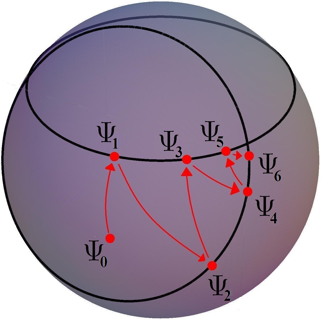
(a)     Convergence for non–complementary observables

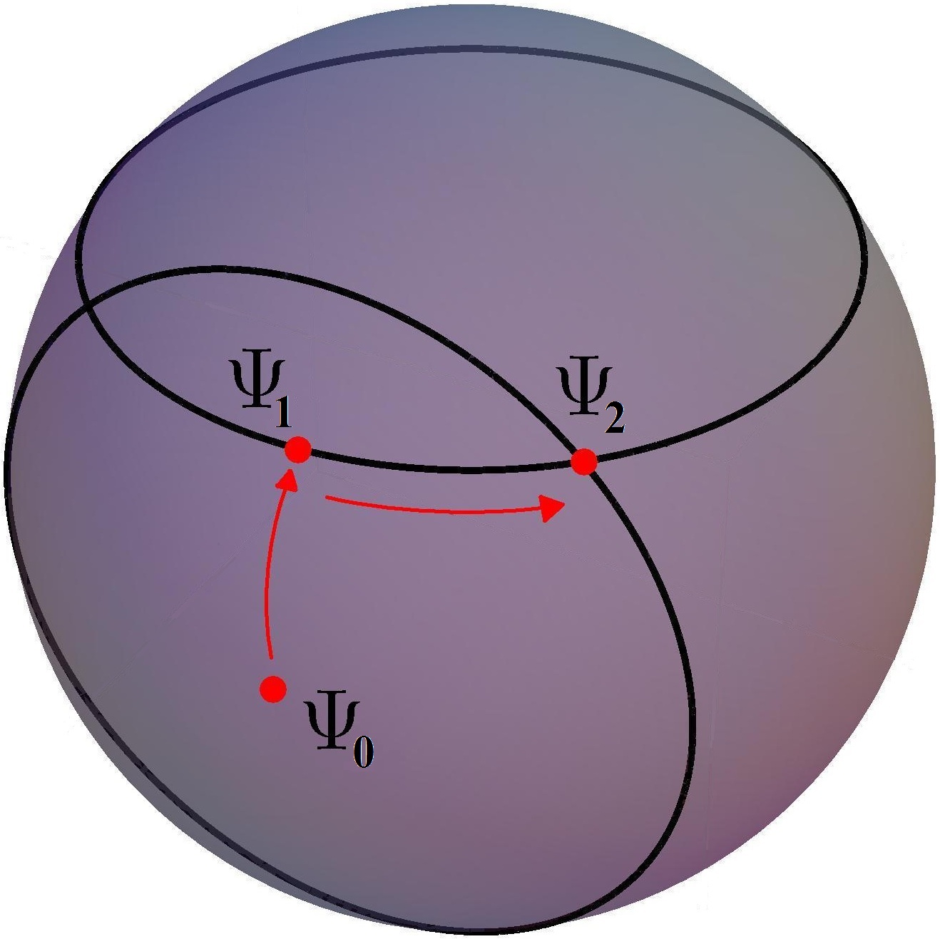
(b)    Convergence for complementary observables

Figure 1: Bloch sphere Representation of the convergence process for the physical imposition operator.

A larger introduction to the physical imposition operator and a detailed study of the convergence criteria of our method can be found in Section III of a previous work Goyeneche5 .

V Bifurcations

Let $A(\alpha)$ be a map depending on the parameters $\alpha$ and $\Gamma(A(\alpha))$ be the set of its fixed points. For some values of $\alpha$, the stability or the number of fixed points may change. In these situations, we say that the map $A$ has a bifurcation Strogatz . In the case of the physical imposition operator the parameters are contained in the generator state $\Phi$ (considering a fixed set of observables). Thus, a bifurcation in the physical fixed points must correspond to a change in the number of physical fixed points in $\Gamma_{A^{1}\cdots A^{m}\Phi}$. This is because the stability of the physical fixed points cannot change (see Prop. IV.6). In order to clarify these ideas let us present a simple example of bifurcations for one qubit state $\Phi\in\mathbb{C}^{2}$: let $S_{x}$, $S_{y}$ and $S_{z}$ be the spin $1/2$ observables. That is,

$$S_{x}=\frac{\hbar}{2}\left(\begin{array}[]{cc}0&1\\ 1&0\\ \end{array}\right),\hskip 14.22636ptS_{y}=\frac{\hbar}{2}\left(\begin{array}[]{cc}0&-i\\ i&0\\ \end{array}\right),\hskip 14.22636pt\mbox{and}\hskip 14.22636ptS_{z}=\frac{\hbar}{2}\left(\begin{array}[]{cc}1&0\\ 0&-1\\ \end{array}\right).$$ (31)

Their eigenvectors bases are given by

$$\mathcal{B}_{x}=\left\{\left(\begin{array}[]{cc}1\\ 0\end{array}\right),\left(\begin{array}[]{cc}0\\ 1\end{array}\right)\right\},\,\mathcal{B}_{y}=\left\{\frac{1}{\sqrt{2}}\left(\begin{array}[]{cc}1\\ 1\end{array}\right),\frac{1}{\sqrt{2}}\left(\begin{array}[]{cc}1\\ -1\end{array}\right)\right\},\,\mathcal{B}_{z}=\left\{\frac{1}{\sqrt{2}}\left(\begin{array}[]{cc}1\\ i\end{array}\right),\frac{1}{\sqrt{2}}\left(\begin{array}[]{cc}i\\ 1\end{array}\right)\right\},$$ (32)

respectively. These orthonormal bases determine a maximal set of three mutually unbiased bases in $\mathbb{C}^{2}$. Two orthonormal bases $\{\varphi_{k}\}$ and $\{\phi_{l}\}$ of $\mathbb{C}^{d}$ are mutually unbiased if

$$|\langle\varphi_{k},\phi_{l}\rangle|^{2}=\frac{1}{d},$$ (33)

for every $k,l=0,\dots,d-1$. Let us consider the physical imposition operator $T_{S_{x}S_{z},\Phi_{1}}$, where $\Phi_{1}\in\mathcal{B}_{x}\cup\mathcal{B}_{z}$. Then, it is easy to show that $T_{S_{x}S_{z},\Phi_{1}}$ has a unique physical fixed point, up to a global unimodular factor. For example, if $\Phi_{1}\in\mathcal{B}_{x}$ then $p^{x}_{k}=\delta_{jk}$, for some $j=0,1$. Therefore, measuring the observable $S_{x}$ it is enough to reconstruct $\Phi$. Indeed, the state of the system is the eigenvector associated to the eigenvalue $s_{j}$ of the observable $S_{x}$. Analogously for $\Phi_{1}\in\mathcal{B}_{z}$. On the other hand, for every $\Phi_{2}\in\mathcal{B}_{y}$ we have

$$p^{x}_{k}=p^{z}_{k}=\frac{1}{2},$$ (34)

for every $k=0,1$. Therefore, the operator $T_{S_{x}S_{z},\Phi_{2}}$ has two physical fixed points, given by the elements of $\mathcal{B}_{y}$. Thus, there exists $\Phi\in\mathcal{H}$ such that $T_{S_{x}S_{z},\Phi}$ has a bifurcation. Moreover, any continuous curve connecting $\Phi_{1}$ with $\Phi_{2}$ contains a generator state producing a bifurcation in $T_{S_{x}S_{z},\Phi}$. Interestingly, bifurcations are manifesting that $S_{x}$ and $S_{z}$ are not informationally complete. On the other hand, if we consider the spin observables $\{S_{x},S_{y},S_{z}\}$ then the physical fixed points of $T_{S_{x}S_{y}S_{z},\Phi}$ does not have bifurcations for any generator $\Phi$ (only for $d=2$). This is because maximal sets of mutually unbiased bases are informationally complete. In the case of $d=3$ the complete set of Pauli partners have been found Goyeneche2 . The example shown above can be generalized to any dimension for a general set of observables:

PROPOSITION V.1

A set of observables $A^{1},\dots,A^{m}$ is informationally complete for pure states iff $T_{A^{1}\cdots A^{m}\Phi}$ has no bifurcations in its physical fixed point for any generator state $\Phi\in\mathcal{H}$.

Proof: Suppose that the observables $A^{1},\dots,A^{m}$ are informationally complete. Therefore, $T_{A^{1}\cdots A^{m}\Phi}$ has always a unique attractive fixed point for any generator state $\Phi$. Moreover, this fixed point cannot change its stability by Prop. IV.6. Then, $T_{A^{1}\cdots A^{m}\Phi}$ has no physical bifurcations. Reciprocally, suppose that $T_{A^{1}\cdots A^{m}\Phi}$ has no physical bifurcations. This means that the number of Pauli partners is the same for any generator state $\Phi$. On the other hand, it is very clear that $\Phi$ is Pauli unique when it is an eigenvector of any of the operators $A^{1},\dots,A^{m}$. Thus, Pauli partners do not exist for any generator state $\Phi$ and $\{A^{1},\dots,A^{m}\}$ is an informationally complete set of observables.   From this proposition the following corollary clearly arises:

COROLLARY V.1

The bifurcations of the physical imposition operators are generated in the eigenvectors of the observables.

Therefore, we realize that bifurcations of the physical imposition operator are the responsible to have multiple solutions to the Pauli problem when an informationally incomplete set of observables is considered. In the case of informationally complete sets of observables there are not bifurcations. The sequence $\{\Psi_{n}\}$ defined in Eq.(29) depends on a seed $\Psi_{0}\in\mathbb{C}^{d}$ that we choose at random in practice. This means that we need to define $2(d-1)$ random numbers and explore a sufficiently large number of seeds $\Psi_{0}$ in order to detect the complete set of physical fixed points. The number of seeds required depends on the generator state, the number of observables, the unbiasedness between the eigenvectors bases of the observables and also depends on the dimension of the Hilbert space. The unbiasedness of a set of orthogonal bases is a measure of how far they are to a set of mutually unbiased bases Durt . Based on several numerical simulations realized in previous works we can affirm that the number of seeds $\Psi_{0}$ required to find the complete set of solutions:

1. Increases with the dimension of $\mathcal{H}$.

2. Decreases with the unbiasedness of the observables.

3. Increases with the distance between the generator $\Phi$ and the closest eigenvector of the observables.

The observables $A^{1},\dots,A^{m}$ are parameters of $T_{A^{1}\cdots A^{m},\Phi}$ that we usually consider as fixed. However, if we fix the generator state $\Phi$ and consider as parameters the observables $A^{1},\dots,A^{m}$ then an interesting result arises from bifurcations theory:

PROPOSITION V.2

If $A^{1},\dots,A^{m}$ is an informationally incomplete set of observables then a small perturbation $A^{1}+\delta A^{1},\dots,A^{m}+\delta A^{m}$ is also informationally incomplete.

Note that the same result can be extended to informationally complete sets of observables iff the physical imposition operator do not have crisis Strogatz . It is possible to make our method more efficient by reducing the number of free parameters of the seed $\Psi_{0}$. This is stated in the following proposition:

PROPOSITION V.3

Let $\Psi_{0}=\sum_{k=0}^{d-1}a_{k}\varphi_{k}$ be a seed, where $\{\varphi_{k}\}$ is the eigenvectors basis of an observable $A^{1}$. Then, the sequence

$$\Psi_{n}=(T_{A^{1}\cdots A^{m},\Phi})^{n}\Psi_{0}=(T_{A^{m},\Phi}\circ\dots\circ T_{A^{1},\Phi})^{n}\Psi_{0},$$ (35)

does not depend on the amplitudes of the seed $\{|a_{k}|\}$.

This proposition has a trivial proof, because the amplitudes $\{|a_{k}|\}$ are missed after applying $T_{A,\Phi}$. Therefore, the number of relevant parameters of the seed $\Psi_{0}$ is reduced from $2(d-1)$ to $d-1$.  

The main disadvantage of our method is that the physical imposition operator, and all its generalizations, have more attractive fixed points than physical ones. This means that some convergent sequences do not correspond to a solution of our problem. Although we are able to recognize the undesirable fixed points we cannot discard them a priory. This problem makes our method less efficient to find solutions in high dimensions, where almost all the time our numerical simulations are discarding non–physical fixed points a posteriori. However, we have successfully found maximal sets of mutually unbiased bases in dimension $d=31$ (992 vectors), genuine multipartite (maximally) entangled pure states up to 8 qubits and complex Hadamard matrices up to dimension 100. The problem to find a fixed point of a composite map $M=M_{1}\circ M_{2}$ which is also a fixed point of $M_{1}$ and $M_{2}$ is known as the split common fixed point problem Censor . It has been proven that an iteration of convex combinations of the form $\lambda M_{1}M_{2}+(1-\lambda)\mathbb{I}$ applied to a given seed successfully converges to a common (attractive) fixed point of $M_{1}$ and $M_{2}$, for some kind of maps. However, this problem is not deeply understood in the literature and it is currently an area of researching.

VI Summary and conclusions

In this work we studied the quantum state reconstruction problem for pure states from the point of view of dynamical systems and bifurcations theory. This novel approach allowed us to find many analytical results and also to develop a powerful tool for finding numerical solutions to geometrical problems in high dimensions. Interestingly, the rate of convergence of our method is much more faster than those obtained by standard methods. We defined the physical imposition operator as the process of imposing information to a blank quantum state (see Def. IV.4). We demonstrated that every solution to the quantum state reconstruction problem is an attractive fixed point of this operator (see Prop. IV.6). We realized that this operator can be adapted to find solutions to many geometrical problems in Hilbert space (mutually unbiased bases, symmetric informationally complete POVM, complex Hadamard matrices, maximally entangled states, etc.). Moreover, the transition to study these problems is straightforward from the results presented in this work. On the other hand, we evidenced the existence of the quantum state reconstruction problem in four independent ways:

• Traditional approach: Multiple solutions for a non–linear system of coupled equations does not have a unique solution (see Eq.(2)).

• Geometrical approach: The inequality between the Bures and distributional metric evidences the existence of the quantum state reconstruction problem (See Prop. III.1).

• Dynamical systems theory approach: The physical imposition operator is a Lipschitz operator having a Lipschitz constant 2 (see 4. in Prop. IV.1). This strongly suggests the existence of the quantum state reconstruction problem.

• Bifurcations theory approach: Bifurcations of the physical imposition operator are associated to multiple solutions to the quantum state reconstruction problem. Bifurcations only appear for informationally incomplete sets of observables (see Prop. V.1). Moreover, bifurcations are generated in the eigenvectors of the observables (see Corollary V.1).

In order to clarify ideas we explained the quantum state reconstruction problem and visualized the convergence of our method in the Bloch sphere (see Fig. 1). Furthermore, the meaning of the physical imposition operator and the concept of informationally completeness were also explained from the Bloch sphere. As an example of informationally complete set we considered a maximal set of three mutually unbiased bases in dimension two. Also, we analyzed the case of two mutually unbiased bases (informationally incomplete) and interpreted the meaning of the Pauli partners in the Bloch sphere. Additionally, an explicit example of bifurcations for two–levels systems has been presented which can be also visualized in the Bloch sphere (see first part in Section V). Finally, we showed that the number of free parameters of the seeds of our method ($\Psi_{0}\in\mathbb{C}^{d}$) can be reduced from $2(d-1)$ to $d-1$ without loosing of generality in every dimension $d$ (see Prop. V.3).

Appendix A

Here, we prove Proposition IV.6. First, we need to prove Proposition IV.1. That is,

PROPOSITION A.1

Let $A$ be an observable having eigenvectors basis $\{\varphi_{k}\}$, $\Phi\in\mathcal{H}$ a generator state and $d(\cdot,\cdot)$ the Bures metric. Then,

1. $d(T_{A\Phi}\Psi,\Psi)\leq d(\Psi,\Phi),\,\forall\,\Phi,\Psi\in\mathcal{H}$.

2. $d(T_{A\Phi}\Psi,\varphi_{k})=d(\Phi,\varphi_{k}),\ \forall\,k=1,\dots,.N$.

3. $d(T_{A\Phi}\Psi,\Phi)\leq 2\min_{k}d(\Phi,\varphi_{k})=2\sqrt{2}\sqrt{1-\max_{k}\sqrt{\rho_{k}}},\ \forall\,\Psi\in\mathcal{H}$.

4. $d(T_{A\Phi}\Psi,\Phi)\leq 2d(\Psi,\Phi),\ \forall\ \Phi,\Psi\in\mathcal{H}$.

5. $T_{A\Phi}\xi=\xi\Leftrightarrow d(T_{A\Phi}\Psi,\xi)\leq d(\Psi,\xi),\ \forall\ \Psi\in N_{A}(\xi)$,

where $N_{A}(\xi)$ is a neighborhood of $\xi$.

proof:

1. $$|\langle T_{A\Phi}\Psi,\Psi\rangle| = \sum_{k=1}^{{N}}|\langle\varphi_{k},\Phi\rangle\langle\varphi_{k},\Psi\rangle|$$ (36)

   $$= \sum_{k=1}^{{N}}|\langle\langle\varphi_{k},\Psi\rangle\,\varphi_{k},\Phi\rangle|$$ (37)

   $$\geq \left|\left\langle\sum_{k=0}^{{N-1}}\langle\varphi_{k},\Psi\rangle\,\varphi_{k},\Phi\right\rangle\right|$$ (38)

   $$= |\langle\Psi,\Phi\rangle|.$$ (39)

   Then,

   $$d(T_{A\Phi}\Psi,\Psi) = \sqrt{2}\sqrt{1-|\langle T_{A\Phi}\Psi,\Psi\rangle|}$$ (40)

   $$\leq \sqrt{2}\sqrt{1-|\langle\Psi,\Phi\rangle|}$$ (41)

   $$= d(\Psi,\Phi).$$ (42)

2. Remembering the definition of the physical imposition operator we can find that

   $$|\langle T_{A\Phi}\Psi,\varphi_{k}\rangle| = \left||\langle\varphi_{k},\Phi\rangle|\frac{\langle\varphi_{k},\Psi\rangle}{|\langle\varphi_{k},\Psi\rangle|}\right|$$ (43)

   $$= |\langle\Phi,\varphi_{k}\rangle|.$$ (44)

   Then,

   $$d(T_{A\Phi}\Psi,\varphi_{k}) = \sqrt{2}\sqrt{1-|\langle T_{A\Phi}\Psi,\varphi_{k}\rangle|}$$ (45)

   $$= \sqrt{2}\sqrt{1-|\langle\Phi,\varphi_{k}\rangle|}$$ (46)

   $$= d(\Phi,\varphi_{k})\ \forall\,k=1,\dots,N.$$ (47)

3. Using the triangular inequality and Eq.(47)

   $$d(T_{A\Phi}\Psi,\Phi)\leq d(T_{A\Phi}\Psi,\varphi_{k})+d(\varphi_{k},\Phi)=2d(\varphi_{k},\Phi),\ \forall\,k=1,\dots,N.$$ (48)

   The most restrictive of the above inequalities is given by

   $$d(T_{A\Phi}\Psi,\Phi)\leq 2\min_{k}d(\varphi_{k},\Phi).$$ (49)

   The equation

   $$\min_{k}d(\varphi_{k},\Phi)=\sqrt{2}\sqrt{1-\max_{k}\sqrt{\rho_{k}}},$$

   is proven immediately from the Bures metric definition.

4. From the triangular inequality and Property 1. of this proposition we have

   $$d(T_{A\Phi}\Psi,\Phi) \leq d(T_{A\Phi}\Psi,\Psi)+d(\Psi,\Phi)$$ (50)

   $$\leq 2d(\Psi,\Phi).$$ (51)

5. Taking into account Eq.(42) and considering the change of parameter $\Psi\rightarrow\xi+\delta\xi$, $\Phi\rightarrow\xi$ we have

   $$d(T_{A\Phi}(\xi+\delta\xi),\xi+\delta\xi)\leq d(\xi+\delta\xi,\xi).$$ (52)

   Note that in the last equation we considered $T_{A\Phi}$ instead of $T_{A\xi}$. This is in order to cover the most general situation. That is, when $\Phi$ is a Pauli partner of $\xi$ and it is not necessarily satisfied that $\Phi=\xi$. Taking $\xi+\delta\xi\in N_{A}(\xi)$ we have

   $$|\langle T_{A\Phi}(\xi+\delta\xi),\xi+\delta\xi\rangle| = |\langle T_{A\Phi}(\xi+\delta\xi),\xi\rangle+\langle T_{A\Phi}(\xi+\delta\xi),\delta\xi\rangle|$$

   $$\approx |\langle T_{A\Phi}(\xi+\delta\xi),\xi\rangle|,$$

   or, equivalently

   $$d(T_{A\Phi}(\xi+\delta\xi),\xi+\delta\xi)\approx d(T_{A\Phi}(\xi+\delta\xi),\xi).$$ (53)

   Thus, considering Eqs.(52) and (53) we have

   $$d(T_{A\Phi}(\xi+\delta\xi),\xi) \approx d(T_{A\Phi}(\xi+\delta\xi),\xi+\delta\xi)$$ (54)

   $$\leq d(\xi+\delta\xi,\xi).$$ (55)

 

Now, we are able to give a proof of Proposition IV.6. From considering the above proposition for the observables $A^{1}\cdots A^{m}$ we have

$$d(\Psi,\xi) \geq d(T_{A^{1}\Phi}\Psi,\xi)$$ (56)

$$\geq d(T_{A^{2}\Phi}T_{A^{1}\Phi}\Psi,\xi)$$ (57)

$$\geq d(T_{A^{3}\Phi}T_{A^{2}\Phi}T_{A^{1}\Phi}\Psi,\xi)$$ (58)

$$\vdots$$ (59)

$$\geq d(T_{A^{m}\Phi}\cdots T_{A^{1}\Phi}\Psi,\xi)$$ (60)

$$\geq d(T_{A^{1}\cdots A^{m}\Phi}\Psi,\xi),$$ (61)

where we consider that $\Psi\in N_{A^{1}\cdots A^{m}}(\xi)=N_{A^{1}}(\xi)\cap\cdots\cap N_{A^{m}}(\xi).$ Then, $\xi$ is an attractive fixed point of $T_{A^{1}\cdots A^{m}\cdots\Phi}$. Notice that the neighborhood $N_{A^{1}\cdots A^{m}}(\xi)$ cannot be a null measure set in state space, because each set $N_{\xi}$ contain an open set around $\xi$. Given that an intersection of a finite number of open sets is an open set, then $N_{ABC\cdots}(\xi)$ contain, at least, an open set. Finally, the basin of attraction of the multiple physical imposition operator contain the set $N_{ABC\cdots}(\xi)$. So, its measure is not null.

References

- (1) W. Pauli, in Quantentheorie, Handbuch der Physik Vol. 24 (Springer, Berlin, 1933), Pt. 1, p. 98.
- (2) J. Amiet, S. Weigert. Reconstructing a pure state of a spin s through three Stern–Gerlach measurements. J. Phys. A 32, 2777-2784 (1999).
- (3) B.Z. Moroz, A.M. Perelomov. On a problem posed by Pauli. Theor. Math. Phys. 101, 1200-1204 (1994).
- (4) D. Gross, Y. Liu, S. Flammia, S. Becker, J. Eisert. Quantum State Tomography via Compressed Sensing. Phys. Rev. Lett. 105, 150401 (2010)
- (5) D. Goyeneche et al. Reconstruction of pure quantum states via five orthonormal bases (Ongoing work).
- (6) J.V. Corbett, C. A. Hurst. Are wave functions uniquely determined by their position and momentum distributions? J. Austral Math. Soc. 20, 182-201 (1978)
- (7) W. Stulpe, M. Singer. Some remarks on the determination of quantum states by measurements. Found. Phys. Lett. 3, 2, 153-166 (1990).
- (8) D. Krahmer, U. Leonhardt. State reconstruction of one–dimensional wave packets. Applied Phys. B, 65, 6, 725-733 (1997)
- (9) J.V. Corbett. The pauli problem, state reconstruction and quantum–real numbers. Reports on Math. Phys. 57, 1, 53 68 (2006)
- (10) P. Jaming, Phase retrieval techniques for radar ambiguity problems, J. Fourier Anal. Appl. 5:4, 309 329 (1999)
- (11) A. Orlowski and H. Paul. Phase retrieval in quantum mechanics. Phys. Rev. A 50, R921 R924 (1994)
- (12) W. Wootters and W. Zurek, Nature 299 (1982) 802.
- (13) I. Ivanovic, J. Phys. A 14, 3241. (1981).
- (14) W. Wootters and B. Fields, Ann. Phys. 191, 363 (1989).
- (15) S. T. Flammia, A. Silberfarb, C. M. Caves, Found. Phys. 35 (2005) 1985.
- (16) T. Heinosaari, L. Mazzarella, M. Wolf. Quantum Tomography under Prior Information. Comm. Math. Phys. 318, 355-374 (2013).
- (17) E. Hellinger. Die Orthogonalinvarianten quadratischer Formen von unendlich vielen Variablen . Dissertation, Göttingen (1907).
- (18) D. M. Goyeneche, A. C. de la Torre. State determination: An iterative algorithm. Phys. Rev. A 77, 042116 (2008).
- (19) D. Goyeneche. Mutually unbiased triplets from non–affine families of complex Hadamard matrices in dimension 6. J. Phys. A: Math. Theor. 46, 105301 (2013)
- (20) D. Goyeneche (ongoing work)
- (21) S. Strogatz. Nonlinear Dynamics And Chaos. Westview Press (2001).
- (22) V. Arnold. Dynamical systems III. Encyclopaedia of Mathematical Sciences, Vol. 3. Springer-Verlag.
- (23) T. Durt, B. Englert, I. Bengtsson, K. Życzkowski. On Mutually unbiased bases. Int. Jour. of Quant. Inf. 8, 4, 535-640 (2010).
- (24) Y. Censor, A. Segal. The Split Common Fixed Point Problem for Directed Operators. J. Convex Anal. 26 055007 (2010)