Multilevel Pricing Schemes in a Deregulated Wireless Network Market

Abstract

Typically the cost of a product, a good or a service has many components. Those components come from different complex steps in the supply chain of the product from sourcing to distribution. This economic point of view also takes place in the determination of goods and services in wireless networks. Indeed, before transmitting customer data, a network operator has to lease some frequency range from a spectrum owner and also has to establish agreements with electricity suppliers. The goal of this paper is to compare two pricing schemes, namely a power-based and a flat rate, and give a possible explanation why flat rate pricing schemes are more common than power based pricing ones in a deregulated wireless market. We suggest a hierarchical game-theoretical model of a three level supply chain: the end users, the service provider and the spectrum owner. The end users intend to transmit data on a wireless network. The amount of traffic sent by the end users depends on the available frequency bandwidth as well as the price they have to pay for their transmission. A natural question arises for the service provider: how to design an efficient pricing scheme in order to maximize his profit. Moreover he has to take into account the lease charge he has to pay to the spectrum owner and how many frequency bandwidth to rent. The spectrum owner itself also looks for maximizing its profit and has to determine the lease price to the service provider. The equilibrium at each level of our supply chain model are established and several properties are investigated. In particular, in the case of a power-based pricing scheme, the service provider and the spectrum owner tend to share the gross provider profit. Whereas, considering the flat rate pricing scheme, if the end users are going to exploit the network intensively, then the tariffs of the suppliers (spectrum owner and service provider) explode.

I Introduction

Optimal pricing mechanisms have been widely studied in networking to control the usage of a sparse resource like frequency bandwidth. In the present work we investigate the following question: what is the impact of the provider pricing mechanism on the decision of each agent in a spectrum supply chain. Often the organization of wireless networks is based on the interaction among several economic entities. For instance, end users pay for a given data rate. Service providers have some costs associated with the wireless network services such as electricity cost, office renting cost, frequency license, etc.

As stated in [1], regulation has been traditionally used in several markets like infrastructure facilities and services. Often after deregulation there is increased competition that in many cases benefits consumers. In [1], the author describes the scope for competition in the major utilities like Electricity, Gas, Railways, Telecommunications, etc. The author shows that the competition is feasible and desirable specifically in telecommunication market. Moreover, in US, collusive behaviours, allowing cartel firms, through a distortion of free market forces, to achieve and share monopolistic profits, are forbidden and persecuted by (not by chance called) ”anti-trust” legislations [2]. That is why in our paper we focus on a deregulation model between the infrastructure provider and the service provider.

To understand the spectrum supply chain problem, we propose to model the system as a multilevel economic game among various agents. Specifically, we consider the following players; the end users, the service provider and the spectrum owner. The spectrum owner has the resource, the spectrum here, and is considered as the top leader in the hierarchy. The service provider rents a quantity of the resource in order to propose services to the end users. The multilevel game approach means that the decision of the spectrum owner is followed by an optimal decision of the service provider, which in turns is followed by an optimal decision of the end users.

Depending on the kind of wireless technology used by the service provider, models of interaction between end users are different. In a first approach, we consider an interference-free model where each end user has his own frequency band to transmit his data. Such kind of phenomenon appears considering Orthogonal Frequency Division Multiplexing (OFDM) technologies [3]. In an alternative approach, we consider a noncooperative power control game between the end users which are interacting together through their signal to interference and noise ratio (SNR). This second model of interaction between the end users corresponds to another wireless technology like code division multiple access (CDMA) [3].

We focus in this paper on a wireless market in which the spectrum owner, called also the infrastructure provider, sells frequency bandwidth to the service provider. This situation is typical in economic models of Cognitive Radio Networks [4]. At a lower level of the spectrum supply chain, the service provider sells services to the end users. The user has his/her utility function and pays according to the transmission rate tariff. The service provider can be seen as a Mobile Virtual Network Operator (MVNO) who obtains spectrum through long-term contracts with spectrum owners or a Mobile Network Operator (MNO). The MVNO resells the spectrum to the end users. MVNOs are mobile service offerings from organizations which typically neither own licensed mobile spectrum nor operate a physical base station network and backhaul. Of course, there are exceptions to the rule but the essential factor is that a MVNO cooperates with a MNO for network access. MNOs are traditional mobile companies such as Orange, SingTel and Vodafone [5]. As stated in [6, 7], it is more efficient for a spectrum owner to hire a MVNO to serve the end users because the MVNO can have a better understanding of local population and user’s demand.Therefore, a natural question arises for the provider: which tariff the service provider has to assign to obtain the maximal pure profit, i.e. the difference between how much he obtains from the end users and how much he has to pay for the licensed frequency bandwidth to the spectrum owner. The spectrum owner who rents part of his spectrum to a MVNO, in turn looks for the frequency bandwidth tariff which can bring to him maximal profit. We focus in our model on a deregulated spectrum market where the resource and the services are not controlled by the same provider, nor by providers which are colluding.

We would like to note that a Stackelberg game approach is very popular among researchers dealing with pricing in networks (see, for example, [8, 9, 10, 11, 12, 13, 14, 15, 16, 17]). In [7], the authors propose a four stage Stackelberg model for the study of spectrum market pricing mechanism with Cognitive MVNO who resells spectrum to secondary users. The authors show some threshold structure of the network equilibrium and fair spectrum allocations to secondary users. The first main difference between the scenario suggested in the present paper and those mentioned above is that we deal with three levels hierarchy users-provider-spectrum owner. Second, we consider different pricing mechanism for the service provider. Finally, we investigate the impact of the interference model between end users on the equilibrium. The major contributions of this paper are described in the following items.

(i)

The power-based pricing mechanism implies the same profit for the service provider and the spectrum owner.

(ii)

The flat rate pricing mechanism induces a higher profit for the service provider compared to the profit of the spectrum owner. It gives a possible explanation to why flat rate pricing schemes are more common than power based pricing ones.

(iii)

A high SINR regime is always desirable in wireless systems to provide quality of service to the end users. Then, assuming this property, we get a simpler closed-form expressions of the equilibrium. Finally, we obtain that the power-based pricing mechanism, assuming high SINR, leads to zero profit for the service provider. Whereas the flat rate pricing mechanism induces non-zero profit for the service provider.

The paper is organized as follows. We present first in section II, the multilevel economic model with the decision set of each agent at each level. In section III we give explicit formulations of the equilibrium in the general wireless context. By assuming a high SINR regime, in section IV, we obtain a closed-form equilibrium and conclude saying that the service provider has to consider the flat rate pricing mechanism instead of the power-based one, in order to maximize his profit. Finally, in Section V and Appendix discussions and sketch of proofs for several theorems are offered.

II Multilevel hierarchical pricing scheme

We introduce a multilevel hierarchical game with the following decision makers: end users, service providers and spectrum owners. The system considered in this paper is a particular multi-level hierarchical supply chain in a wireless network. In fact we consider first that at the lower level, with the longest time scale, each end user determines his transmit power in order to maximize selfishly his utility function. Second, a service provider, at the middle level and intermediate time scale, rents some frequencies from the spectrum owner in order to provide services to the users. Then the service provider determines optimally the quantity of bandwidth to rent to end users and the tariff end user should pay for their services. Third, the spectrum owner, at a longer level and shorter time scale, manages the spectrum and determines the price of a unit of bandwidth rent by the service provider. In terms of timescale, our system considers three different timescales. The shorter one is the spectrum owner one who decides the tariff per unit of frequency bandwidth the service provider has to pay for. In telecommunication market, this timescale can be like several years. A second longer timescale is the service provider’s one, which determines the quantity of bandwidth to rent and the tariff each end users have to pay for their services. This second timescale is the order of a year. Finally, the longest timescale is the end users one who choose their transmit power with a timescale of some months or days or minutes, depending on the wireless technology used. Note that this power control management should be implemented into communication protocols in end-users devices. The main objective of our model is to study this multilevel supply chain in wireless telecommunication market, not to necessary obtain any practical implementation or software, but to understand the behavior of the different decision makers in such a complex economic system.

The three-level optimization problem can be described more formally as follows from the spectrum owner (top-level) to the end users (low-level).

(i) The spectrum owner maximizes his revenue $v_{A}(W,C_{W})=C_{W}W$ depending on the tariff $C_{W}$ per unit of frequency bandwidth assigned to the service provider, i.e.

$$\max_{C_{W}}v_{A}(W,C_{W})=\max_{C_{W}}C_{W}W,$$ (1)

where $W$ is the quantity of bandwidth chosen by the servi ce provider.

(ii) In order to maximize his payoff $v_{P}(C_{P},W,C_{W})$, the service provider determines the quantity of bandwidth $W$ to license from the spectrum owner and the tariff $C_{P}$ the end users have to pay for their services i.e.

$$\max_{W,C_{P}}v_{P}(C_{P},W,C_{W})=\max_{W,C_{P}}\left\{C_{P}\sum_{i=1}^{n}\mu(T_{i})-C_{W}W\right\},$$ (2)

where the function $\mu(\cdot)$ is the pricing scheme used by the service provider, which depends on user’s $i$ transmission power $T_{i}$ and $n$ is the number of end users.

(iii) Finally, each end user $i$ determines his transmission power $T_{i}$ in order to maximize his net utility $u_{i}(\mbox{\boldmath$T$},C_{P})$ with $\mbox{\boldmath$T$}=(T_{1},\ldots,T_{n})$ which is the difference between the throughput and the price imposed by the service provider, i.e.

$$\max_{T_{i}}u_{i}(\mbox{\boldmath$T$},C_{P})=\max_{T_{i}}\left\{W\ln\left(1+\gamma_{i}(\mbox{\boldmath$T$})\right)-C_{P}\mu(T_{i})\right\},$$ (3)

where $\gamma_{i}(\mbox{\boldmath$T$})$ is the signal to noise ratio (SNR) on user’s $i$ signal. This function determines the quality of the signal received and then can used to approximate the capacity of a wireless link with bandwidth $W$ based on the Shannon formula [18, 19]. This utility function is well-known in the literature on pricing schemes in wireless systems like in [8].

In order to compute the solutions of this multilevel game, we use a step-by-step approach from the low-level optimization problem (the end users) to the high-level one (the spectrum owner). The solution of this three-level game is a hierarchical (Stackelberg) equilibrium [20].

In the first step, for a fixed usage tariff $C_{P}$ and bandwidth $W$, determined by the service provider, the $n$ users compete by trying to maximize selfishly their own payoff. We deal here with a homogeneous network, namely, we assume that all the users are in the same wireless conditions (so, they have the same restriction on power and the same fading gains). Each of them can be considered as an average user. Homogeneous network suits considering the network where average users operate and since we try to give an explanation why flat rating is more common we can restrict ourself to such network. In our future work we are going to investigate what impact on pricing schemes different types of user’s groups can produce, say, employing different applications or have different objectives [21, 22].

It is natural when studying a power control problem, to consider that a strategy of a user $i$ is the transmitted power $T_{i}\in[0,\overline{T}]$ with $\overline{T}$ is the maximal (average) power a user can apply.

In the second step of the multilevel game, the service provider, knowing that the end users will act as it was described in the fist step, chooses for the optimal tariff $C_{P}$ and how much frequency bandwidth $W$ to license from the spectrum owner. The service provider payoff $v_{P}$ is the difference between how much he earns from selling services to the users and how much he has to pay for the licensed frequency bandwidth.

In the third step of the multilevel game, the spectrum owner selects the optimal tariff $C_{W}$ it has to assign to get the maximal profit.

The aim of the paper is to study this multilevel economic model with two pricing schemes for the service provider: one flat rate and the other one power-based. A flat fee, also referred to as a flat rate or a linear rate, refers to a pricing structure that charges a single fixed fee for a service, regardless of usage. Then, the pricing function defined in equation (1) is $\mu(x)=1$. For Internet service providers, a flat rate pricing scheme determines an access to the Internet for all customers of the telco operator at a fixed tariff. Flat rate is common in broadband access to the Internet in the USA and many other countries. In the power-based pricing scheme, we consider that the profit of the service provider comes from the network usage and it is proportional to the total power used by all the end users to send their traffic. Then, our model tends to limit the power of the end users as they have to pay the provider not based on the throughput they use but the power they consume. In this case, the service provider consider uses the following function $\mu(T_{i})=T_{i}$. Note that introducing power based cost is common for CDMA [23, 24] and ALOHA networks ([25, 26]).

III General wireless model

We assume a standard wireless communication model as proposed in [3], where the signal received at the base station can be written as $y=hx+z$, where $h$ stands for the block fading process, $x$ the signal transmitted by the end user and $z$ is the additive Gaussian noise. We assume coherent communication such that the fading channel gain is constant over each block fading length. Moreover, the additive Gaussian noise $z$ at the receiver is i.i.d circularly symmetric and $z\sim\mathcal{CN}(0,\sigma^{2})$. Two wireless scenarios are considered: interference-free and interference channel.

III-A Interference-free model

We consider the situation where the end users have access to the network interference from other end users, like in an Orthogonal Frequency Division Multiplexing (OFDM) wireless technology in which each end user has his own transmission frequency. So, there is no interference between end users since the service provider supplies different bandwidth frequency for each end user. Then, the signal-to-noise ratio (SNR) of each end user $i$ is given by $\gamma_{i}=\frac{LhT_{i}}{(W/n)\sigma^{2}}$ where $T_{i}$ is user’s $i$ transmit power and $L$ is the crosstalk coefficient. We assume a symmetric system such that all end users have the same channel gain $h$. Moreover the service provider shares the leased bandwidth frequency $W$ equally between the end users. Then we assume that user $i$’s utility is given as follows:

$$u_{i}(T_{i})=(W/n)\ln\left(1+LhT_{i}/(W\sigma^{2}/n)\right)-C_{P}\mu(T_{i}).$$ (4)

For the flat-rate pricing scheme, i.e. $\mu(x)=1$, it is natural to assume that each end user is going to consume all the capacity. Indeed the utility function $u_{i}$ is strictly increasing depending on $T_{i}$. Then, each end user transmits with the maximal power $\overline{T}$. Using this transmission power, each end user gets a throughput equals to $\frac{W}{n}\ln\left(1+\frac{Lh\overline{T}}{(W/n)\sigma^{2}}\right)$ and has to pay $C_{P}$ for the service. Then, each end user accepts the provider’s service if his utility (the difference between the throughput and the charge) is non-negative. Indeed, there is no incentive to transmit if his net utility is negative as it is generally assume in economic models in telecommunication [27]. Moreover, since the service provider intends to maximize his profit, then

$$C_{P}=(W/n)\ln\left(1+Lh\overline{T}/(W\sigma^{2}/n)\right).$$ (5)

We have the first result supplying the solution of the multilevel supply chain spectrum problem for flat-rate and power based pricing schemes with interference-free model.

Theorem 1

If there is no interference between end users, the equilibrium solution of the multilevel economic problem $(C_{W},W,C_{P},\mbox{\boldmath$T$})$ and corresponding payoffs of the service provider and the spectrum owner are given in Table I.

TABLE I: The optimal solution for interference-free model

	Power based pricing	Flat rate pricing
$C_{W}$	$\frac{1}{4}$	$\approx 0.468$
$W$	$\frac{nLh\overline{T}}{\sigma^{2}}$	$\approx\frac{0.462nLh\overline{T}}{\sigma^{2}}$
$C_{P}$	$\frac{Lh}{2\sigma^{2}}$	$\approx\frac{0.532Lh\overline{T}}{\sigma^{2}}$
$T$	$(\overline{T},\ldots,\overline{T})$	$(\overline{T},\ldots,\overline{T})$
$v_{P}$	$\frac{nLh\overline{T}}{4\sigma^{2}}$	$\approx\frac{0.316nLh\overline{T}}{\sigma^{2}}$
$v_{A}$	$\frac{nLh\overline{T}}{4\sigma^{2}}$	$\approx\frac{0.216nLh\overline{T}}{\sigma^{2}}$

First, one important remark is that the optimal frequency bandwidth tariffs $C_{W}^{PB-IF}=0.25$ and $C_{W}^{FR-IF}=0.468$, for both pricing schemes, do not depend on the number $n$ of end users nor network’s parameters. Here and below, upper indexes FR-IF and PB-IF mean flat rate and power based pricing schemes for the interference-free model correspondingly. Moreover, power-based tariff is almost twice less $C_{W}^{FR-IF}/C_{W}^{PB-IF}\approx 1.87$. Considering the power-based pricing scheme the provider and the spectrum owner share profit equally $v^{PB-IF}_{A}=v^{PB-IF}_{P}=\frac{\displaystyle nhL\overline{T}}{\displaystyle 4\sigma^{2}}$ meanwhile, with the flat rate pricing scheme, the service provider’s payoff is essentially greater than the spectrum owner’s one, i.e. $v^{PB-IF}_{A}/v^{PB-IF}_{P}=1.462$. Then, using a power-based pricing scheme, the market is shared equally between the service provider and the spectrum owner, whereas a flat-rate pricing scheme makes the service provider’s payoff higher than the spectrum owner’s payoff. Moreover, the total profit $v_{P}+v_{A}$ generated for both decision makers, the service provider and the spectrum owner, is higher with the flat rate pricing scheme, i.e. $\frac{0.532nLh\overline{T}}{\sigma^{2}}$, compared to the total profit with the power-based pricing scheme, i.e. $\frac{0.5nLh\overline{T}}{\sigma^{2}}$. Finally, surprisingly, each end user chooses also to transmit using maximum power, even if a power-based pricing is used by the provider instead of a flat rate pricing scheme. Thus, we can conclude that from one hand, in the context of non-interfering end users, a power-based pricing scheme will not help the spectrum owner to control the total power consumption of the network but will permit for him to get more market share and then earn more revenue from the spectrum rent. From the other hand, the flat rate pricing scheme is preferable for the service provider since it brings him higher profit compared to using a power based pricing scheme which is moreover, more difficult to build in practice.

III-B Interference channels

In this section we consider that the access to the network is performed considering user’s interference. The signal to interference and noise ratio (SINR) $\gamma_{i}$ of end user $i$ is given by

$$\gamma_{i}(\mbox{\boldmath$T$})=LhT_{i}\bigr{/}\left(W\sigma^{2}+h\sum_{j=1,j\not=i}^{n}T_{j}\right).$$

We consider a symmetric system, then the block fading process is the average one and it is the same for all users. So, the end user’s $i$ payoff depends on the user action $T_{i}$ and also on the actions of the other end users. We denote by $T_{-i}$ the vector of the actions of all the other players $j\neq i$. The end user’s $i$ payoff becomes

$$u_{i}(\mbox{\boldmath$T$})=W\ln\left(1+\gamma_{i}(\mbox{\boldmath$T$})\right)-C_{P}\mu(T_{i}).$$

For a fixed usage tariff $C_{P}$, the vector of end user’s strategies $\mbox{\boldmath$T$}^{*}$ is a Nash equilibrium (NE) if, by definition [20],

$$\forall i\in\{1,\ldots,n\},\quad\forall T_{i}\in[0,\overline{T}],\quad u_{i}(T^{*}_{i},\mbox{\boldmath$T$}^{*}_{-i})\geq u_{i}(T_{i},\mbox{\boldmath$T$}^{*}_{-i}),$$

where $\mbox{\boldmath$T$}_{-i}$ is the vector of all the end users instead user $i$. We have the next result supplying the solution of the multilevel supply chain spectrum problem for flat-rate and power based pricing schemes with interfering end users. We take into consideration then the NE between the end users for a given decision of the service provider and the spectrum owner.

Theorem 2

If there is interference between end users, the solution of the multilevel economic problem $(C_{W},W,C_{P},\mbox{\boldmath$T$})$ and corresponding payoffs $v_{P}$ and $v_{A}$ to the provider and the spectrum owner are given in Table II.

TABLE II: The optimal solution for interference channels model

	Power based pricing	Flat rate pricing
$W$	$\frac{(n+L-1)h\overline{T}}{\sigma^{2}}$	$W(C_{W})=\arg\max_{W<\left(\frac{L}{\exp(C_{W}/n)-1}+1-n\right)\frac{h\bar{T}}{\sigma^{2}}}\left(n\ln\left(1+\frac{Lh\overline{T}}{W\sigma^{2}+h(n-1)\overline{T}}\right)-C_{W}\right)W$
$C_{W}$	$\frac{nL}{4(n+L-1)}$	$C_{W}=\arg\max_{C_{W}<n\ln(1+L/(n-1))}C_{W}W(C_{W})$
$C_{P}$	$\frac{Lh}{2\sigma^{2}}$	$W(C_{W})\ln\left(1+\frac{Lh\overline{T}}{W(C_{W})\sigma^{2}+(n-1)h\overline{T}}\right)$
T	$(\overline{T},\ldots,\overline{T})$	$(\overline{T},\ldots,\overline{T})$
$v_{P}$	$\frac{nLh\overline{T}}{4\sigma^{2}}$	$nW(C_{W})\ln\left(1+\frac{Lh\overline{T}}{W(C_{W})\sigma^{2}+(n-1)h\overline{T}}\right)-C_{W}\,W(C_{W})$
$v_{A}$	$\frac{nLh\overline{T}}{4\sigma^{2}}$	$C_{W}\,W(C_{W})$

For the power based pricing scheme in interference model the optimal frequency bandwidth tariff $C_{W}$ is increasing on number of users and the quality of network $L$. Specifically, this value tends to $L/4$ when increasing the number of end users and converges to $n/4$ when increasing the quality of network $L$. Second, we observe also that the demand $W$ at the equilibrium from the service provider in frequency bandwidth is increasing depending on the number of end users $n$ to serve. Finally, the network is over loaded such that the equilibrium user’s strategies T is to use the maximum power. Then, it looks like there is some kind of inside cooperative stimulus of all the participants of the market (they just split the common profit) who are in charge for network functionality and going to meet all the user’s demands. We conclude by observing the utility of each decision maker at the equilibrium.

• The profit of the spectrum owner and the profit of the service provider coincide at the equilibrium, namely, $v_{A}=v_{P}=\frac{\displaystyle nhL\overline{T}}{\displaystyle 4\sigma^{2}}$. Thus, the spectrum owner assigns the bandwidth frequency tariff in order to withdraw from the service provider a fixed percent (namely, fifty percent) of his gross profit.

• For each end user $i$, the optimal utility is given as follows

  $$u_{i}=\frac{\overline{T}h}{2\sigma^{2}}\left(2(n+L-1)\ln\left(2\frac{n+L-1}{2n+L-2}\right)-L\right).$$

  which corresponds the following user’s throughput

  $$R=\frac{\overline{T}h(n+L-1)}{\sigma^{2}}\ln\left(2\frac{n+L-1}{2n+L-2}\right).$$

  Thus,(since function $f(\xi)=\xi\ln(\xi/(\xi-L))$ is decreasing from infinity for $\xi\downarrow L$ to $L$ while $\xi$ tends to infinity) the utility of each end user is strictly decreasing with $n$ and converges to 0 if $n$ tends to infinity. Moreover, the throughput of each end user is decreasing with $n$ but converges to the lower bound $\overline{T}hL/(2\sigma^{2})$. Thus, whatever the number of end users is, the throughput of each end used is lower bounded, meaning that automatically a best-effort service can be provided.

• Figures 1 and  2 demonstrate that the most profitable pricing scheme for the service provider is the flat rate pricing scheme when considering end user’s interference. It allows the spectrum owner to increase bandwidth cost (and it continuously increasing up to its upper-bound $L/4$) While transmission cost even drops down by the provider a bit for the flat rate pricing scheme, or it keeps on the same level ($Lh/(2\sigma^{2})$) for power base pricing scheme. All together it leads to increasing in the provider’s and spectrum owner’s profits. Increasing consumption of the maximal power by end-users (which can be described as increasing intension of using the network by them) without increasing number of end users also allows the provider and spectrum owner to increase their profits, but they manage to get it a bit different way. The spectrum owner’does not increase the bandwidth cost for both pricing schemes and gains just due to increasing demands in bandwidth. Meanwhile the provider to cover the extra expanses to buy more bandwidth has to lift up cost in flat rate scheme. In power based pricing scheme the extra income obtained due to more intensive using the network by end users allows the provider to buy more bandwidth for higher price without increasing transmission cost.

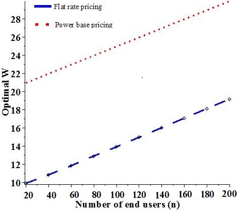
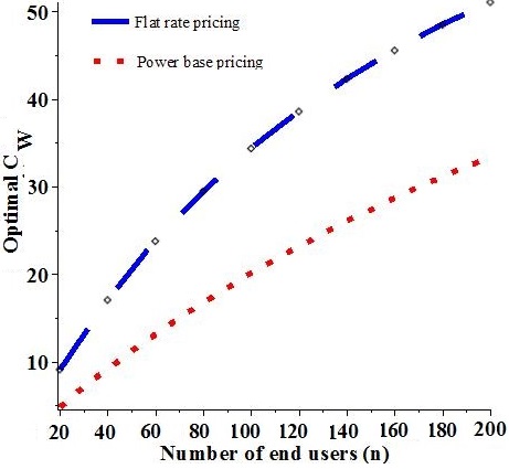
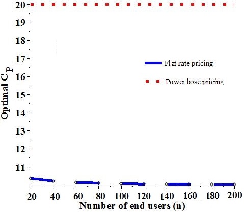
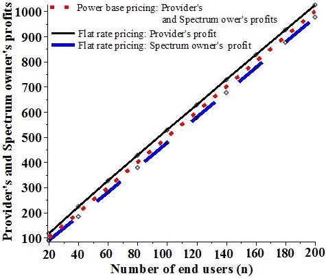
(a)	(b)	(c)	(d)

Figure 1: (a) The optimal bandwidth $W$, (b) the optimal bandwidth cost $C_{W}$, (c) the optimal transmission cost $C_{P}$ and (d) the provider’s and spectrum owner’s payoffs as functions on number of end users $n$ with $L=400$, $h=1$, $\bar{T}=0.5$ and $\sigma^{2}=10.$

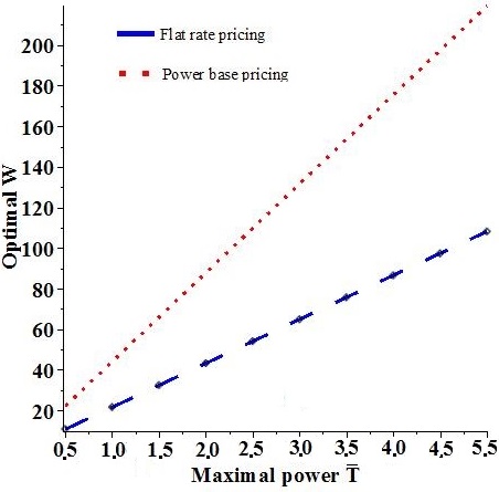
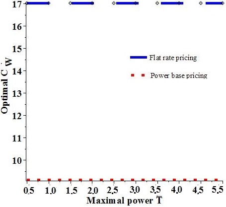
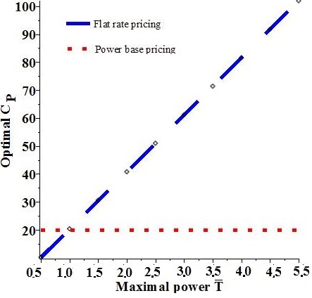
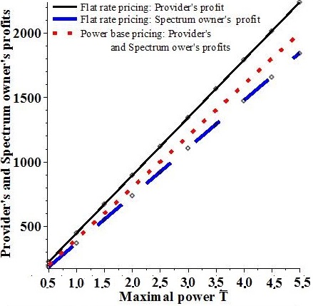
(a)	(b)	(c)	(d)

Figure 2: (a) The optimal bandwidth $W$, (b) the optimal bandwidth cost $C_{W}$, (c) the optimal transmission cost $C_{P}$ and (d) the provider’s and spectrum owner’s payoffs as functions on maximal power $\bar{T}$ with $L=400$, $h=1$, $n=40$ and $\sigma^{2}=10.$

IV Special case: high SNR regime

A particular interesting wireless context is the high SNR regime, i.e. for each end user $i$, $\gamma_{i}>>1$. This assumption is always desirable in wireless networks (see [28] for a recent paper on performance of multiplexing MIMO systems in high-SNR regime) and leads to the following relation $T_{i}>>\frac{W\sigma^{2}}{nLh}$ which gives a lower bound on user’s $i$ transmission power. Moreover, this assumption has been also proposed in [7] for the study of an optimal pricing mechanism for spectrum in a cognitive radio context. This bound is relatively small as the number of end users $n$ is large and then, this lower bound is realistic in a wireless network. Thus, assuming high SNR regime, we have that $1+\gamma_{i}$ can be approximated by $\gamma_{i}$. Then for the interference-free model, the end user’s $i$ payoff, assuming high SNR regime, is approximated by the following expression

$$u_{i}(\textbf{T})=\frac{W}{n}\ln\left(\frac{LhT_{i}}{(W/n)\sigma^{2}}\right)-C_{P}\mu_{i}(T_{i})$$

and for the interference user model it is given as follows

$$u_{i}(\textbf{T})=W\ln\left(\frac{LhT_{i}}{W\sigma^{2}+h\sum_{j=1,j\not=i}^{n}T_{j}}\right)-C_{P}\mu_{i}(T_{i}).$$

To deal with high SNR approximation considering the power-based pricing scheme, we assume that the bandwidth which the spectrum owner can sell to the service provider is upper-bounded, namely, that $W<\overline{W}$. Then we have the next result supplying the solution of the multilevel supply chain spectrum game for flat-rate and power based pricing schemes, and considering the high SNR assumption.

Theorem 3

Considering high SNR assumption, the equilibrium of the multilevel economic problem $(C_{W},W,C_{P},\textbf{T})$ and corresponding payoffs $v_{P}$ and $v_{A}$ for the service provider and the spectrum owner are given in Table III where $\epsilon$ is any enough small positive .

TABLE III: The equilibrium of the multilevel spectrum game in high SNR regime.

	Power based	Power based	Flat rate	Flat rate
	Interference-free	Interference	Interference-free	Interference
$C_{W}$	$1-\epsilon$	$n-\epsilon$	$1$	$n\mbox{LambertW}^{2}\left(\frac{n-1}{L}e^{\frac{n+C_{W}}{n}}\right)+C_{W}=n$
$W$	$\overline{W}$	$\overline{W}$	$\approx\frac{0.135nLh\overline{T}}{\sigma^{2}}$	$W=\frac{(n-1)h\overline{T}}{\sigma^{2}}\left(\frac{1}{\mbox{LambertW}\left(\frac{n-1}{L}e^{\frac{n+C_{W}}{n}}\right)}-1\right)$
$C_{P}$	$\overline{W}/(\overline{T}n)$	$\overline{W}/\overline{T}$	$\approx\frac{0.271Lh\overline{T}}{\sigma^{2}}$	$W\ln\left(\frac{Lh\overline{T}}{W\sigma^{2}+(n-1)h\overline{T}}\right)$
$v_{P}$	$\overline{W}\epsilon$	$\overline{W}\epsilon$	$\approx\frac{0.135nLh\overline{T}}{\sigma^{2}}$	$nW\ln\left(\frac{Lh\overline{T}}{W\sigma^{2}+(n-1)h\overline{T}}\right)-C_{W}W$
$v_{A}$	$\overline{W}(1-\epsilon)$	$\overline{W}(n-\epsilon)$	$\approx\frac{0.135nLh\overline{T}}{\sigma^{2}}$	$C_{W}W$

It is quite interesting that considering the power-based pricing scheme, the spectrum owner withdraws all the profit from the service provider, just leaving him a bit, i.e. $\overline{W}\epsilon$, to keep working in the business. For the flat rate pricing scheme, the spectrum owner and the service provider share the total profit. Also, it is interesting to note that for the interference-free model at high SNR regime, the spectrum tariff $C_{W}^{FR-IF-H}$ of the spectrum owner is more than twice higher than the one in general regime $C_{W}^{FR-IF}$ since

$$C_{W}^{FR-IF-H}/C_{W}^{FR-IF}=1/0.468=2.14.$$

Meanwhile, when the end users are going to exploit the network intensively, the tariff applied by the service provider

$$C_{P}^{FR-IF-H}/C_{P}^{FR-IF}=0.271/0.532=0.51$$

is reduced two times. The service provider’s payoff reduces also since

$$v_{P}^{FR-IF-H}/v_{P}^{FR-IF}=0.135/0.315=0.429.$$

We can conclude this remark by saying that if the service provider does not control the number of end users and if this number becomes large, using an OFDM technology the noise can be very low for each end user and then his SNR very high. Thus, the provider’s payoff is divided by 2.

V Conclusions

In this paper, we have studied a multilevel economic model of wireless networks with two pricing schemes: a flat-rate or a power-based. The different decision makers are the end users, a service provider and a spectrum owner. The proposed economic model can be applied in several networking contexts like cognitive radio network, where a company or an authority which has the control on the resource (the spectrum here) rents frequencies to service providers and at the end of this spectrum supply chain, end users pay for their services to the service providers. This multilevel model gives interesting results on how optimal economic relations are built between the different decision makers. In particular, for the power-based pricing scheme, the service provider and the spectrum owner split equally the total market profit. Whereas, considering a flat-rate pricing scheme it is more profitable for the service provider. Of course this conclusion should be taken with caution, and that a more complete model is needed to make stronger conclusions. In terms of quality of service, the power-based tariff at the equilibrium depends on the quality of the network and not on the number of end users. Another important result deals with the flat-rate pricing scheme. Considering this scheme, if the end users are going to exploit the network intensively then, it leads to double increasing of the bandwidth frequency tariff by the spectrum owner. It leads also to a bit less than double increasing of the flat rate tariff to the end users applied by the service provider. Also, we show that power-based pricing leads to an equal profit split between spectrum owner and provider, and that the power-based pricing can lead to the spectrum owner getting more profit than a flat-pricing scheme even though flat-pricing is better for extracting the surplus from the users. In future works, we plan to investigate that kind of multilevel model for a important new wireless market by considering Cognitive Radio Networks in which second hand wireless providers can sell spectrum holes to secondary users.

VI Appendix

VI-A Proof of Theorem 1

We consider the flat rate pricing scheme, i.e. $\mu(x)\equiv 1$. Then, the utility of each end users is strictly increasing with the transmission power $T$, and thus each end will use the maximum power $\overline{T}$. Moreover, each end-user accepts the provider’s service if and only if his utility is positive, which gives the maximum tariff an end-user is able to pay:

$$C_{P}=\frac{W}{n}\ln\left(1+\frac{Lh\overline{T}}{(W/n)\sigma^{2}}\right).$$

Given this, the provider’s payoff turns into the following function:

$$v_{P}(C_{P},W,C_{W})=W\ln\left(1+\frac{nh\overline{T}L}{W\sigma^{2}}\right)-C_{W}W.$$

Note that this function does not depend on $C_{P}$ and:

$$\frac{\partial v_{P}}{\partial W}(C_{P},W,C_{W})=\ln\left(1+\frac{Lh\overline{T}n}{W\sigma^{2}}\right)-\frac{Lh\overline{T}n}{Lh\overline{T}n+W\sigma^{2}}-C_{W}.$$

We look now for the optimal quantity of bandwidth the provider will rent from the spectrum provider depending on the tariff $C_{W}$. The optimal frequency bandwidth to lease is given as follows:

$$W=W(C_{W}):=-\frac{(Lh\overline{T}n/\sigma^{2})\mbox{LambertW}(-e^{-1-C_{W}})}{1+\mbox{LambertW}(-e^{-1-C_{W}})}.$$ (6)

Finally, the spectrum owner’s payoff can be rewritten depending only on $C_{W}$ as follows:

$$\begin{split}v_{A}(C_{W})=-\frac{(Lh\overline{T}n/\sigma^{2})\mbox{LambertW}(-e^{-1-C_{W}})}{1+\mbox{LambertW}(-e^{-1-C_{W}})}C_{W}.\end{split}$$

Note that the derivative of this function is:

$$\begin{split}\frac{dv_{A}(C_{W})}{dC_{W}}&=(Lh\overline{T}n/\sigma^{2})\mbox{LambertW}\left(-e^{-1-C_{W}}\right)\\ &\times\frac{C_{W}-\left(1+\mbox{LambertW}\left(-e^{-1-C_{W}}\right)\right)^{2}}{(1+\mbox{LambertW}(-e^{-1-C_{W}}))^{3}}.\end{split}$$

So, the optimal bandwidth frequency tariff is given as the root of the equation

$$C_{W}-\left(1+\mbox{LambertW}\left(-e^{-1-C_{W}}\right)\right)^{2}=0.$$

and then since $C_{W}\approx 0.468$ the result follows for the flat rate pricing scheme.

We consider the power based pricing scheme, i.e. $\mu(x)\equiv x$. At the first step of the multilevel game, we have to find the optimal end user strategies. To do so, we first determine the optimal transmission power of each end user $i$ by computing the derivative of his utility function:

$$\frac{du_{i}}{dT_{i}}(T_{i})=\frac{\displaystyle WLh}{\displaystyle W\sigma^{2}+LhnT_{i}}-C_{P}.$$

Thus, the optimal transmission power of user $i$ is $T_{i}=T(C_{P},W)$:

$$T(C_{P},W)=\begin{cases}\overline{T},&\displaystyle C_{P}\leq\frac{\displaystyle LWh}{\displaystyle W\sigma^{2}+Lhn\overline{T}},\\ \frac{\displaystyle W}{\displaystyle n}\left(\frac{\displaystyle 1}{\displaystyle C_{P}}-\frac{\displaystyle\sigma^{2}}{\displaystyle Lh}\right),&\frac{\displaystyle LWh}{\displaystyle W\sigma^{2}+Lhn\overline{T}}<C_{P}<\frac{\displaystyle Lh}{\displaystyle\sigma^{2}},\\ 0,&\frac{\displaystyle Lh}{\displaystyle\sigma^{2}}\leq C_{P}.\end{cases}$$ (7)

Now we consider the second step where the provider, knowing the equilibrium user’s strategies (7) have to decide which tariff $C_{P}$ to assign and how much bandwidth $W$ to lease to maximize his revenue. The provider’s payoff at the second step of the game is given by:

$$\begin{split}v_{P}&(C_{P},W)=-C_{W}W\\ &+\begin{cases}n\overline{T}C_{P},&\displaystyle C_{P}\leq\frac{\displaystyle LWh}{\displaystyle W\sigma^{2}+Lhn\overline{T}},\\ W\left(1-\frac{\displaystyle\sigma^{2}C_{P}}{\displaystyle Lh}\right),&\frac{\displaystyle LWh}{\displaystyle W\sigma^{2}+Lhn\overline{T}}<C_{P}<\frac{\displaystyle Lh}{\displaystyle\sigma^{2}},\\ 0,&\frac{\displaystyle Lh}{\displaystyle\sigma^{2}}\leq C_{P}.\end{cases}\end{split}$$ (8)

Then, the provider’s revenue achieves its maximum value when the tariff for the users $C_{P}$ is such that

$$C_{P}=C_{P}(W):=\frac{\displaystyle LWh}{\displaystyle W\sigma^{2}+Lhn\overline{T}}.$$ (9)

Substituting (9) into (8) leads to the following expression of the provider’s revenue depending only on the quantity of bandwidth $W$ to lease:

$$\begin{split}v_{P}(C_{P},W)=v_{P}(W):=\frac{\displaystyle n\overline{T}LWh}{\displaystyle W\sigma^{2}+Lhn\overline{T}}-C_{W}W.\end{split}$$ (10)

The derivative of this expression depending on $W$ is:

$$\begin{split}\frac{dv_{P}}{dW}(W)&=\frac{(Lnh\overline{T})^{2}(1-C_{W})-2Lnh\overline{T}C_{W}W-C_{W}\sigma^{4}W^{2}}{\left(W\sigma^{2}+Lnh\overline{T}\right)^{2}}.\end{split}$$

Then,

(a) if $C_{W}\geq 1$ then $v_{P}(W)$ is decreasing for positive $W$,

(b) if $C_{W}<1$ then $v_{P}(W)$ is increasing on the interval $\left(0,(1-\sqrt{C_{W}})\overline{T}hnL/(\sqrt{C_{W}}\sigma^{2})\right)$ and it is decreasing on the interval $\left((1-\sqrt{C_{W}})\overline{T}hnL/(\sqrt{C_{W}}\sigma^{2}),\infty\right)$.

Thus, the optimal bandwidth $W=W(C_{W})$ which maximizes the provider’s revenue is given as follows:

$$W(C_{W})=\begin{cases}0,&C_{W}\geq 1,\\ \frac{\displaystyle(1-\sqrt{C_{W}})\overline{T}hnL}{\displaystyle\sqrt{C_{W}}\sigma^{2}},&C_{W}<1.\end{cases}$$ (11)

Then, at the third and last step of the game, taking into account (11) the spectrum owner’s payoff is given by

$$\begin{split}v_{A}(C_{W})=\begin{cases}0,&C_{W}\geq 1,\\ \frac{\displaystyle\sqrt{C_{W}}(1-\sqrt{C_{W}})\overline{T}hnL}{\displaystyle\sigma^{2}},&C_{W}<1.\end{cases}\end{split}$$

Then, the optimal spectrum owner’s strategy maximizing $v_{A}(C_{W})$ is to assign the frequency bandwidth tariff $C_{W}=1/4$, and the result follows.  

VI-B Proof of Theorem 2

We consider the flat rate pricing scheme, i.e. $\mu(x)\equiv 1$. It is clear that the end users optimal behaviour is $\textbf{T}=(\overline{T},\ldots,\overline{T})$. Then, for the provider, the tariff in order to maximize his payoff is:

$$C_{P}=C_{P}(W):=W\ln\left(1+\frac{Lh\overline{T}}{W\sigma^{2}+h(n-1)\overline{T}}\right).$$

Thus, the provider’s payoff at the NE of the end users becomes:

$$\begin{split}v_{P}(C_{P},W,C_{W})&=v_{P}(C_{P}(W),W,C_{W})=nC_{P}-WC_{W}\\ &=\left(n\ln\left(1+\frac{Lh\overline{T}}{W\sigma^{2}+h(n-1)\overline{T}}\right)-C_{W}\right)W.\end{split}$$

Then,

$$\ \arg\limits_{W}\max v_{P}(C_{P}(W),W,C_{W})\begin{cases}=0,&C_{W}\geq n\ln\left(1+\frac{\displaystyle L}{\displaystyle n-1}\right),\\ >0,&C_{W}<n\ln\left(1+\frac{\displaystyle L}{\displaystyle n-1}\right),\end{cases}$$

and the result follows.

We consider the power based pricing scheme, i.e. $\mu(x)\equiv x$. As usual in hierarchical optimization problems, in order to compute a solution, we consider the optimization problem starting from the bottom optimization level (the end users equilibrium) to the top level optimization problem (the spectrum owner).

At the first step we have to find the Nash equilibrium of the non-cooperative power control game between the end users. The utility function of end user $i$ is given by:

$$u_{i}(\textbf{T})=W\ln\left(1+\frac{LhT_{i}}{W\sigma^{2}+h\sum_{j=1,j\not=i}^{n}T_{j}}\right)-C_{P}T_{i}.$$

In order to obtain the Nash equilibrium, we determine the best-response strategy of each end user by computing the following partial derivative:

$$\frac{\partial u_{i}}{\partial T_{i}}(\textbf{T})=\frac{\displaystyle WLh}{\displaystyle W\sigma^{2}+LhT_{i}+h\sum_{j=1,j\not=i}^{n}T_{j}}-C_{P}.$$

Thus, as the game is symmetric, the equilibrium strategy $T_{i}=T(C_{P},W)$ for each user $i$ is

$$T(C_{P},W)=\begin{cases}\overline{T},&\displaystyle C_{P}\leq\frac{\displaystyle LWh}{\displaystyle W\sigma^{2}+(n-1+L)h\overline{T}},\\ \frac{\displaystyle\left(\frac{\displaystyle Lh}{\displaystyle C_{P}}-\sigma^{2}\right)W}{\displaystyle h(n-1+L)},&\frac{\displaystyle LWh}{\displaystyle W\sigma^{2}+(n-1+L)h\overline{T}}<C_{P}\\ &\mbox{and }C_{P}<\frac{\displaystyle Lh}{\displaystyle\sigma^{2}},\\ 0,&\frac{\displaystyle Lh}{\displaystyle\sigma^{2}}\leq C_{P}.\end{cases}$$ (12)

At the second step, the provider, knowing the equilibrium user’s strategies (12), has to determine which tariff $C_{P}$ to assign and how much bandwidth $W$ to lease in order to maximize his revenue. The provider’s payoff at the second step of the game is given by:

$$\begin{split}&v_{P}(C_{P},W)=-C_{W}W\\ &+\begin{cases}n\overline{T}C_{P},&\displaystyle C_{P}\leq\frac{\displaystyle LWh}{\displaystyle W\sigma^{2}+(n-1+L)h\overline{T}},\\ \frac{\displaystyle\left(Lh-\sigma^{2}C_{P}\right)nW}{\displaystyle h(n-1+L)},&\frac{\displaystyle LWh}{\displaystyle W\sigma^{2}+(n-1+L)h\overline{T}}<C_{P}\\ &\mbox{and }C_{P}<\frac{\displaystyle Lh}{\displaystyle\sigma^{2}},\\ 0,&\frac{\displaystyle Lh}{\displaystyle\sigma^{2}}\leq C_{P}.\end{cases}\end{split}$$ (13)

Then, the provider revenue $v_{P}(C_{P},W)$ is continuous and piece-monotonous on $C_{P}$ such way that

(a) $v_{P}(C_{P},W)$ is increasing for $C_{P}\leq\frac{LWh}{W\sigma^{2}+(n-1+L)h\overline{T}},$

(b) $v_{P}(C_{P},W)$ is decreasing for $\frac{LWh}{W\sigma^{2}+(n-1+L)h\overline{T}}<C_{P}<\frac{Lh}{\sigma^{2}}$,

(c) $v_{P}(C_{P},W)$ is constant for $\frac{Lh}{\sigma^{2}}\leq C_{P}$.

Then, the provider revenue achieves its optimum value when the tariff for the users $C_{P}$ is such that

$$C_{P}=C_{P}(W):=LWh/\left(W\sigma^{2}+(n-1+L)h\overline{T}\right).$$ (14)

Substituting (14) into (13) leads to the following expression of the provider’s revenue depending only on the quantity of bandwidth $W$ to lease:

$$\begin{split}v_{P}(W):=v_{P}(C_{P}(W),W)=\frac{\displaystyle nLWh\overline{T}}{\displaystyle W\sigma^{2}+(n-1+L)h\overline{T}}-C_{W}W.\end{split}$$ (15)

Note that the derivative depending on $W$ of the provider’s revenue is:

$$\begin{split}\frac{dv_{P}}{dW}(W)=\frac{A_{2}W^{2}+A_{1}W+A_{0}}{(W\sigma^{2}+h(n+L-1)\overline{T})^{2}},\end{split}$$

with

$$\begin{split}A_{0}&:=h^{2}\overline{T}^{2}(n+L-1)(nL-C_{W}(n+L-1)),\\ A_{1}&:=-2C_{W}\sigma^{2}h\overline{T}(n+L-1),\\ A_{2}&:=-C_{W}\sigma^{2}.\end{split}$$

The following equation $A_{2}W^{2}+A_{1}W+A_{0}=0$ has the two roots:

$$W_{\pm}=(-C_{W}(n+L-1)\pm\sqrt{C_{W}nL(n+L-1)})\frac{\overline{T}h}{C_{W}\sigma^{2}}.$$

Then we have the following cases:

(a)

if $C_{W}\geq\frac{nL}{L+n-1}$ then $v_{P}(W)$ is decreasing for positive $W$,

(b)

if $C_{W}<\frac{nL}{L+n-1}$ then $v_{P}(W)$ is increasing for $W<W_{+}$ and decreasing for $W>W_{+}$.

Thus, the optimal bandwidth $W=W(C_{W})$ which maximizes the provider’s revenue is given as follows:

$$W(C_{W})=\begin{cases}0,&C_{W}\geq\frac{\displaystyle nL}{\displaystyle L+n-1},\\ (\sqrt{nL}-\sqrt{C_{W}nL(n+L-1)})\\ \times\frac{\displaystyle\sqrt{(n+L-1)}\overline{T}h}{\displaystyle\sqrt{C_{W}}\sigma^{2}},&\mbox{otherwise}.\end{cases}$$ (16)

Finally, at the third and last step of the game, taking into account (16), the spectrum owner’s payoff is given by:

$$\begin{split}v_{A}(C_{W})=\begin{cases}0,&C_{W}\geq\frac{\displaystyle nL}{\displaystyle L+n-1},\\ \frac{\displaystyle\sqrt{C_{W}(n+L-1)}\overline{T}h}{\displaystyle\sigma^{2}}\\ \times(\sqrt{nL}-\sqrt{C_{W}nL(n+L-1)}),&\mbox{otherwise}.\end{cases}\end{split}$$

If $C_{W}<\frac{\displaystyle nL}{\displaystyle L+n-1}$ we have that

$$\frac{dv_{A}}{dC_{W}}(C_{W})=\frac{\overline{T}h\sqrt{n+L-1}}{2\sigma^{2}\sqrt{C_{W}}}(\sqrt{nL}-2\sqrt{C_{W}(n+L-1)}).$$

Then, the optimal spectrum owner’s strategy is to assign the frequency bandwidth tariff $C_{W}$ as follows: $C_{W}=\frac{nL}{4(n+L-1)}$ and the result follows.  

VI-C Proof of Theorem 3

We consider the flat rate pricing scheme, i.e. $\mu(x)=1$ in user-free model. Considering the high SNR regime, we can make the following approximation $\log(1+\gamma_{i})=\log(\gamma_{i})$. Then the provider’s payoff becomes:

$$v_{P}(C_{P},W,C_{W})=W\ln\left(\frac{Lnh\overline{T}}{W\sigma^{2}}\right)-WC_{W}.$$

Note that the derivative of the provider’s payoff is:

$$\begin{split}\frac{\partial v_{P}}{\partial W}(C_{P},W,C_{W})=\ln\left(\frac{Lhn\overline{T}}{W\sigma^{2}}\right)-1-C_{W}.\end{split}$$

Thus, the optimal frequency bandwidth $W=W(C_{W})$ to lease is

$$W(C_{W}):=\frac{Lhn\overline{T}}{\sigma^{2}e^{1+C_{W}}}.$$

The spectrum owner’s payoff turns into the following expression:

$$\begin{split}v_{A}(C_{W})&=C_{W}W(C_{W})=\frac{Lhn\overline{T}C_{W}}{\sigma^{2}e^{1+C_{W}}}.\end{split}$$

Note that the derivative of this function is:

$$\begin{split}\frac{dv_{A}}{dC_{W}}(C_{W})=\frac{Lhn\overline{T}(1-C_{W})}{\sigma^{2}e^{1+C_{W}}}.\end{split}$$

Then, the optimal bandwidth frequency tariff is $C_{W}=1$ and the optimal quantity of bandwidth rent by the provider is:

$$W=\frac{Lhn\overline{T}}{\sigma^{2}e^{2}}$$

and the result follows:

We consider the flat rate pricing scheme, i.e. $\mu(x)=1$ in interference model. Given the approximation of the SINR of each end users, the provider’s revenue is given by:

$$v_{P}(C_{P},W,C_{W})=nW\ln\left(\frac{Lh\overline{T}}{W\sigma^{2}+h(n-1)\overline{T}}\right)-WC_{W}.$$

Note that the derivative of this expression depending on the quantity of bandwidth $W$ is:

$$\begin{split}\frac{\partial v_{P}}{\partial W}(C_{P},W,C_{W})&=n\ln\left(\frac{Lh\overline{T}}{W\sigma^{2}+(n-1)h\overline{T}}\right)\\ &-\frac{W\sigma^{2}n}{W\sigma^{2}+(n-1)h\overline{T}}-C_{W}.\end{split}$$

Thus, the optimal frequency bandwidth to lease is $W=W(C_{W})$ with

$$W(C_{W}):=\frac{(n-1)h\overline{T}}{\sigma^{2}}\left(\frac{\displaystyle 1}{\displaystyle\mbox{LambertW}\left(\frac{\displaystyle n-1}{\displaystyle L}e^{\frac{\displaystyle n+C_{W}}{\displaystyle n}}\right)}-1\right).$$

Given the optimal reaction of the provider, the spectrum owner’s payoff can be rewritten by:

$$\begin{split}v_{A}(C_{W})=\frac{(n-1)h\overline{T}}{\sigma^{2}}\left(\frac{\displaystyle 1}{\displaystyle\mbox{LambertW}\left(\frac{\displaystyle n-1}{\displaystyle L}e^{\frac{\displaystyle n+C_{W}}{\displaystyle n}}\right)}-1\right)C_{W}.\end{split}$$

We compute the derivative of this function:

$$\begin{split}\frac{dv_{A}(C_{W})}{dC_{W}}&=\frac{1-\mbox{LambertW}^{2}\left(\frac{\displaystyle n-1}{\displaystyle L}e^{\frac{\displaystyle n+C_{W}}{\displaystyle n}}\right)-C_{W}}{\mbox{LambertW}\left(\frac{\displaystyle n-1}{\displaystyle L}e^{\frac{\displaystyle n+C_{W}}{\displaystyle n}}\right)}\\ &\times\frac{\displaystyle(n-1)h\overline{T}/\sigma^{2}}{1+\mbox{LambertW}\left(\frac{\displaystyle n-1}{\displaystyle L}e^{\frac{\displaystyle n+C_{W}}{\displaystyle n}}\right)}.\end{split}$$

So, the optimal bandwidth frequency tariff is given as the root of the equation

$$\mbox{LambertW}^{2}\left(\frac{\displaystyle n-1}{\displaystyle L}e^{\frac{\displaystyle n+C_{W}}{\displaystyle n}}\right)=1-C_{W}.$$

and the result follows.

We consider the power based pricing scheme, i.e. $\mu(x)=x$ in interference model. First we have to find the Nash equilibrium of the non-cooperative power control game between the end users. The utility function of end user $i$ is given by:

$$u_{i}(\mbox{\boldmath$T$})=W\ln\left(\frac{LhT_{i}}{W\sigma^{2}+h\sum_{j=1,j\not=i}^{n}T_{j}}\right)-C_{P}T_{i}.$$

In order to obtain the Nash equilibrium, we determine the best-response strategy of each end user by computing the following partial derivative:

$$\frac{\partial u_{i}}{\partial T_{i}}(\textbf{T})=\frac{\displaystyle W}{\displaystyle T_{i}}-C_{P}.$$

Thus, the user’s Nash equilibrium is $(\overline{T},\ldots,\overline{T})$ and the optimal tariff is $C_{P}=C_{P}(W)=W/\overline{T}$. Thus, the payoffs to the provider and spectrum owner turn into $v_{P}(W,C_{W})=(n-C_{W})W$, $v_{A}(W,C_{W})=C_{W}W$, and the result follows.

We consider the power based pricing scheme, i.e. $\mu(x)=x$ in user-free model. First we have to find the Nash equilibrium of the non-cooperative power control game between the end users. The utility function of end user $i$ is given by:

$$u_{i}(\textbf{T})=\frac{W}{n}\ln\left(\frac{nLhT_{i}}{W\sigma^{2}}\right)-C_{P}T_{i}.$$

In order to obtain the Nash equilibrium, we determine the best-response strategy of each end user by computing the following partial derivative:

$$\frac{\partial u_{i}}{\partial T_{i}}(\textbf{T})=\frac{\displaystyle W}{\displaystyle nT_{i}}-C_{P}.$$

Thus, the user’s Nash equilibrium is $(\overline{T},\ldots,\overline{T})$ and the optimal tariff is $C_{P}=C_{P}(W)=W/\overline{T}$. Thus, the payoffs to the provider and spectrum owner turn into $v_{P}(W,C_{W})=(1-C_{W})W$, $v_{A}(W,C_{W})=C_{W}W$, and the result follows.

References

- [1] The Economic Regulation of Transport Infrastructure Facilities and Services. United Nations, 2001.
- [2] D. Sama, Competition Law, Cartel Enforcement and Leniency Program. LUISS Guido Carli University of Rome, 2008.
- [3] V. Garg, Wireless Communications and Networking. Morgan Kaufmann Publishers, 2010.
- [4] E. Hossain, D. Niyato, and Z. Han, Dynamic Spectrum Access and Management in Cogntive Radio Networks. Cambridge University Press, 2009.
- [5] The MVNO Directory 2011. 2011.
- [6] R. Dewenter and J. Haucap, “Incentives to licence virtual mobile network operators (MVNOs),” in Proceedings of the 34th Res. Conf. Comm., 2006.
- [7] L. Duan, J. Huang, and B. Shou, “Investment and pricing with spectrum uncertainty: A cognitive operator’s perspective,” IEEE Transactions on Mobile Computing, vol. 10, no. 11, pp. 1590–1604, 2011.
- [8] A. A. Daoud, T. Alpcan, S. Agarwal, and M. Alanyali, “A stackelberg game for pricing uplink power in wide-band cognitive radio networks,” in Proceedings of IEEE CDC 2008, pp. 1422–1427, 2008.
- [9] T. Basar and R. Shrikant, “Revenue-maximizimg pricing and capacity expansion in a many-users regime,” in Proceedings of IEEE Infocom 2002, vol. 1, pp. 294–301, 2002.
- [10] F. Bernstein and A. Federgruen, “A general equilibrium model for industries with price and service competition,” Operations Research, vol. 52, no. 6, pp. 868–886, 2004.
- [11] L. Duan, J. Huang, and B. Shou, “Cognitive mobile virtual network operator: Investment and pricing with supply uncertainty,” in Proceedings of IEEE Infocom 2010, pp. 1–9, 2010.
- [12] A. Garnaev, Y. Hayel, K. Avrachenkov, and E. Altman, “Throughput and QoS pricing in wireless communication,” in Proceedings of the 5th International ICST Conference on Performance Evaluation Methodologies and Tools ( ValueTools ’11), pp. 362–371, 2011.
- [13] A. Garnaev, Y. Hayel, K. Avrachenkov, and E. Altman, “Optimal hierarchical pricing schemes for wireless network usage and resource allocation,” in Proceedings of the 4th Workshop on Network Control and Optimization (NET-COOP 2010), pp. 60–65, 2010.
- [14] P. Maille, B. Tuffin, and J. Vigne, “Economics of technological games among telecommunication service providers,” Journal of Communications and Networks, vol. 21, pp. 65–82, 2011.
- [15] J. Musacchio, G. Schwartz, and J. Walrand, “A two-sided market analysis of provider investment incentives with an application to the net-neutrality issue,” Review of Network Economics, vol. 8, 2009.
- [16] D. Niyato and E. Hossain, “Optimal price competition for spectrum sharing in cognitive radio: A dynamic game-theoretic approach,” in Proceedings of IEEE Globecom 2007, pp. 4625–4629, 2007.
- [17] A. Galegov and A. Garnaev, “How hierarchical structures impact on competition,” AUCO Czech Economic Review, vol. 2, no. 3, pp. 227–236, 2008.
- [18] C. Shannon, “A mathematical theory of communication,” Bell Syst. Techn. J., vol. 27, pp. 379–423, 1948.
- [19] B. Rengarajan, A. Stolyar, and H. Viswanathan, A Semi-autonomous Algorithm for Self-organizing Dynamic Fractional Frequency Reuse on the Uplink of OFDMA Systems. Bell Labs Technical Memo, 2009.
- [20] D. Fudenberg and J. Tirole, Game Theory. MIT Press, 1991.
- [21] A. Garnaev, W. Trappe, and C.-T. Kung, “Dependence of optimal monitoring strategy on the application to be protected,” in Proceedings of IEEE Globecom 2012, pp. 1054–1059, 2012.
- [22] A. Garnaev, W. Trappe, and C.-T. Kung, “Optimizing scanning strategies: Selecting scanning bandwidth in adversarial RF environments,” in Proceedings of 8th International Conference on Cognitive Radio Oriented Wireless Networks (CROWNCOM 2013), pp. 148–153, 2013.
- [23] Q. Zhu, W. Saad, Z. Han, H. Poor, and T. Basar, “Eavesdropping and jamming in next-generation wireless networks: a game-theoretic approach,” in Proceedings of Military Communications Conference (MILCOM 2011), pp. 119–124, 2011.
- [24] E. Altman, K. Avrachenkov, and A. Garnaev, “Taxation for green communication,” in Proceedings of the 8th International Symposium on Modeling and Optimization in Mobile, Ad Hoc and Wireless Networks (WiOpt 2010), pp. 108–112, 2010.
- [25] Y. Sagduyu and A. Ephremides, “A game-theoretic analysis of denial of service attacks in wireless random access,” Journal of Wireless Networks, vol. 15, pp. 651–666, 2009.
- [26] A. Garnaev, Y. Hayel, E. Altman, and K. Avrachenkov, “Jamming game in a dynamic slotted ALOHA network,” in Game Theory for Networks (R. Jain and R. Kannan, eds.), vol. 75 of LNICST, pp. 429–443, Springer, 2012.
- [27] O. Korcak, T. Alpcan, and G. Iosifidis, “Collusion of operators in wireless spectrum markets,” in Proceedings of WiOpt 2012, pp. 33–40, 2012.
- [28] L. Ordonez, D. Palomar, A. Pages-Zamora, and J. Fonollosa, “High-SNR analytical performance of spatial multiplexing MIMO systems with CSI,” IEEE Transactions on Signal Processing, vol. 55, pp. 5447–5463, 2007.