Rotational Behaviors and Magnetic Field Evolution of Radio Pulsars

Abstract

The observed long-term spin-down evolution of isolated radio pulsars cannot be explained by the standard magnetic dipole radiation with a constant braking torque. However how and why the torque varies still remains controversial, which is an outstanding problem in our understanding of neutron stars. We have constructed a phenomenological model of the evolution of surface magnetic fields of pulsars, which contains a long-term decay modulated by short-term oscillations; a pulsar’s spin is thus modified by its magnetic field evolution. The predictions of this model agree with the precisely measured spin evolutions of several individual pulsars; the derived parameters suggest that the Hall drift and Hall waves in the NS crusts are probably responsible for the long-term change and short-term quasi-periodical oscillations, respectively. Many statistical properties of the timing noise of pulsars can be well re-produced with this model, including correlations and the distributions of the observed braking indices of the pulsars, which span over a range of more than 100 millions. We have also presented a phenomenological model for the recovery processes of classical and slow glitches, which can successfully model the observed slow and classical glitch events without biases.

1 Introduction

A radio pulsar is a rotating neutron star (NS) with strong surface magnetic fields, which emits a beam of electromagnetic radiation along the axis of the fields. Much resembling the way of a lighthouse, the radiation can only be seen when the light is pointed to the direction of an observer. Since a NS is a very stable rotator, it produces a series of pulses with a very precise interval that ranges from milliseconds to seconds in the radio band.

The arrival times of the pulses can be recorded with very high precision. Indeed, thanks to the high precision, a surprising amount can be learned from them (see Lyne & Graham-Smith 2012). As early as the first pulsar was discovered (on November 28, 1967), Hewish and his collaborators noticed that they provide the information that not only the radio source might be a rotating NS, but also about its position and motion, as well as the dispersion effect during the pulses’ propagation through the interstellar medium (Hewish el al. 1968).

The time-of-arrival (TOA) measurements now give the precise information on various modes of the spin evolution of individual NSs, and on the orbits and rotational slowdown of binary pulsars, and thus made possible some fundamental tests of general relativity and gravitational radiation. Some millisecond pulsars with rather stable pulsations (even challenging the best atomic clocks), are used as a system of Galactic clocks for ephemeris time or gravitational wave detection.

The variations of spin frequency $\nu$ and its first derivative $\dot{\nu}$ of pulsars are obtained from polynomial fit results of arriving time epochs (i.e. phase sequences) of pulses. Since the rotational period is nearly constant, these observable quantities, $\nu$, $\dot{\nu}$ and $\ddot{\nu}$ can be obtained by fitting the phases to the third order of its Taylor expansion over a time span $t_{\rm s}$,

$$\Phi_{i}={\Phi}+\nu(t_{i}-t)+\frac{1}{2}\dot{\nu}(t_{i}-t)^{2}+\frac{1}{6}\ddot{\nu}(t_{i}-t)^{3}.$$ (1)

One can thus get the values of $\nu$, $\dot{\nu}$ and $\ddot{\nu}$ at $t$ from fitting to Equation (1) for independent $N$ data blocks around $t$, i.e. $i=1,...,N$.

The most obvious feature of a pulsar spin evolution is that it is observed to slow down gradually, i.e. $\dot{\nu}<0$. According to classical electrodynamics, a inclined magnetic dipole in vacuum lose its rotational energy via emitting low-frequency electromagnetic radiation. Assuming the pure magnetic dipole radiation as the braking mechanism (e.g. Lorimer 2004), we have

$$\dot{\nu}=-AB_{0}^{2}\nu^{3},$$ (2)

in which $A=8\pi^{2}R^{6}\sin\theta^{2}/3c^{3}I$ is a constant, $B_{0}$ is the strength of the dipole magnetic fields at the surface of the NS, $R~{}(\simeq 10^{6}~{}{\rm cm})$, $I~{}(\simeq 10^{45}~{}{\rm g~{}cm^{2}})$, and $\theta~{}(\simeq\pi/2)$ are the radius, moment of inertia, and angle of magnetic inclination from the rotation axis, respectively. Though the energy flow from a pulsar may be a combination of this dipole radiation and an outflow of particles, Equation (4) is still valid, since the magnetic energy dominate the total energy of the outer magnetosphere (Lyne & Graham-Smith 2012).

Figure 1: Observed correlation between $\ddot{\nu}$ and $3\dot{\nu}^{2}/\nu$. The prediction of the standard magnetic dipole radiation model, i.e., $\ddot{\nu}=3\dot{\nu}^{2}/\nu$ is shown as the dashed line, which under-predicts significantly the magnitudes of $\ddot{\nu}$ for most pulsars and also cannot explain $\ddot{\nu}<0$ for nearly half of the pulsars. All the data are taken from Hobbs et al. (2010), and the figure is taken from Paper I.

Following Equation (4) and assuming $\dot{B}_{0}=0$, the frequency’s second derivative can be simply expressed as

$$\ddot{\nu}=3\dot{\nu}^{2}/\nu.$$ (3)

The model predicts $\ddot{\nu}>0$ and $|\ddot{\nu}|$ should be very small. However, as shown in Figure 1 (Zhang & Xie 2012a; hereafter Paper I), the observed $\ddot{\nu}$ is often significantly different from the model predictions, so that the braking mechanism may be oversimplified. However how and why the torque varies still remains controversial, which is an outstanding problem in our understanding of neutron stars.

In this paper, we give a brief review for the phenomenological model we constructed recently, and its applications on the spin behaviors of pulsars, which include the statistical properties of $\ddot{\nu}$ and $n_{\rm b}$, and the dipole magnetic field evolution of some individual pulsars, as well as their physical implications on NS interiors. A phenomenological model for glitch recoveries of individual pulsars are also briefly discussed.

2 The phenomenological model

To model the discrepancy between the observed $\ddot{\nu}$ and the predicted $\ddot{\nu}$ by Equation (3), the braking law of a pulsar is generally assumed as

$$\dot{\nu}=-K\nu^{n_{\rm b}},$$ (4)

where $n_{\rm b}$ is called its braking index. Manchester & Taylor (1977) gave that

$$n_{\rm b}=\ddot{\nu}\nu/\dot{\nu}^{2},$$ (5)

if $\dot{K}=0$. For the standard magnetic dipole radiation model with constant magnetic field ($\dot{K}=0$), Equation (3) applies and yields $n_{\rm b}=3$. Therefore $n_{\rm b}\neq 3$ indicates some deviation from the standard magnetic dipole radiation model with constant magnetic fields.

Blandford & Romani (1988) re-formulated the braking law of a pulsar as,

$$\dot{\nu}=-K(t)\nu^{3}.$$ (6)

This means that the standard magnetic dipole radiation is responsible for the instantaneous spin-down of a pulsar, but the braking torque determined by $K(t)$ may be variable. In this formulation, $n_{\rm b}\neq 3$ does not indicate deviation from the standard magnetic dipole radiation model, but means only that $K(t)$ is time dependent. Assuming that magnetic field evolution is responsible for the variation of $K(t)$, we have $K=AB(t)^{2}$, in which $B(t)$ is the time variable dipole magnetic field strength of a pulsar. The above equation then suggests that $n_{\rm b}<3$ indicates magnetic field growth of a pulsar, and vice versa, since $\dot{\nu}<0$ and $K>0$. This can be seen more clearly from (Paper I and Zhang & Xie 2012b (Paper II)),

$$\dot{K}=\frac{\dot{\nu}^{2}}{\nu^{4}}(3-n_{\rm b}).$$ (7)

Equation (6) cab be re-written as

$$\dot{\nu}\nu^{-3}=-AB(t)^{2},$$ (8)

and the time scale of the magnetic field long-term evolution of each pulsar (see Equation (6) in Paper I) is given by

$$\tau_{B}\equiv\frac{B}{\dot{B}}=\frac{2\dot{\nu}_{0}\nu_{0}}{\ddot{\nu}_{\rm L}\nu_{0}-3\dot{\nu}_{0}^{2}}.$$ (9)

$\tau_{B}<0$ indicates magnetic field decrease and vice versa.

In Paper I and II, we constructed a phenomenological model for the dipole magnetic field evolution of pulsars with a long-term decay modulated by short-term oscillations,

$$B(t)=B_{\rm d}(t)(1+\sum k_{i}\sin(\phi_{i}+2\pi\frac{t}{T_{i}})),$$ (10)

where $t$ is the pulsar’s age, and $k_{i}$, $\phi_{i}$, $T_{i}$ are the amplitude, phase and period of the $i$-th oscillating component, respectively. $B_{\rm d}(t)=B_{0}(t/t_{0})^{-\alpha}$, in which $B_{0}$ is the field strength at the age $t_{0}$, and $\alpha$ is the power law index.

By substituting Equation (10) into Equation (8) and taking only the dominating oscillating component, we obtained the analytic approximation for $\dot{\nu}$ (Xie & Zhang 2013c, hereafter Paper V):

$$\dot{\nu}\simeq\dot{\nu}_{0}(1+2k(\sin(\phi+2\pi\frac{t}{T})-\sin\phi))+\ddot{\nu}_{\rm L}(t-t_{0}),$$ (11)

where $\dot{\nu}_{0}=\dot{\nu}(t_{0})$, $\ddot{\nu}_{\rm L}=-2\alpha\dot{\nu}_{0}/t_{0}$ describes the long-term monotonic variation of $\dot{\nu}(t)$. Therefore Equation (11) can be tested with the long-term monitoring observations of individual pulsars. If the long-term observed average of $\ddot{\nu}$ is approximately given by the expression for $\ddot{\nu}_{\rm L}$ above (i.e. $\langle\ddot{\nu}\rangle\simeq\ddot{\nu}_{\rm L}$), then we can use the previously reported $\ddot{\nu}$ obtained from the timing solution fits of the whole data span as an estimate of $\ddot{\nu}_{\rm L}$.

Similarly we also find (Paper I)

$$\ddot{\nu}\simeq-2\dot{\nu}(\alpha/t_{\rm age}+fC(t)),$$ (12)

where $t_{\rm age}$ is the real age of the pulsar, $f\equiv 2\pi k/T$ for the dominating oscillating component, and $C(t)=\cos(\phi+2\pi\frac{t}{T})$. For relatively young pulsars with $t_{\rm age}<3\times 10^{5}$ yr, the first term in Equation (12) dominates and we should have $\ddot{\nu}>0$ if $\alpha>0$. Considering that the characteristic ages ($\tau_{\rm c}$) of young pulsars are normally several times larger than $t_{\rm age}$, Equation (12) thus explains naturally the observed $\ddot{\nu}>0$ for most young pulsars with $\tau_{\rm c}<10^{6}$ yr.

Without other information about $t$, we replace it with the magnetic age of a pulsar $t=t_{0}(B_{0}/B)^{(1/\alpha)}$ in Equation (12); we then have,

$$\ddot{\nu}\simeq\eta(-\dot{\nu})^{1+\beta}/\nu^{3\beta}+2\dot{\nu}fC(t),$$ (13)

where $\beta=1/2\alpha$, $\eta=(3.3\times 10^{19}/B_{0})^{2\beta}/\beta t_{0}$ and $B=3.3\times 10^{19}\sqrt{P\dot{P}}$ G is assumed. Thus the model predicts a correlation between $\ddot{\nu}$ and $(-\dot{\nu})^{1+\beta}/\nu^{3\beta}$ for young pulsars with $\tau_{\rm c}<10^{6}$ yr. Similarly for much older pulsars, the second term in Equation (12) dominates, in agreement with the observational fact that the numbers of negative and positive $\ddot{\nu}$ are almost equal for the old pulsars.

From Equation (8), we can also obtain,

$$n_{\rm b}=3+\frac{\tau_{\rm c}}{t}(2-4ftC(t)).$$ (14)

As we have shown in Paper I, the oscillatory term can be ignored in determining $\ddot{\nu}$, so young pulsars with $\tau_{\rm c}\leq 10^{5}$ should have $n_{\rm b}>0$, consistent with observations.

3 Dipole magnetic field evolution of individual pulsars

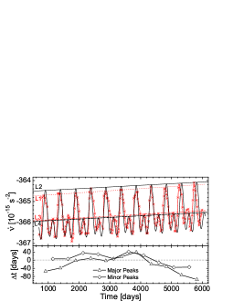
Figure 2: Upper Panel: $\dot{\nu}(t)$ for PSR B1828$-$11 during the past 20 years. The reported data are represented by red stars; and the solid black line is calculated from Equation (11). Lower Panel: Time differences between the peak positions of reported data and analytical calculation. The figure is taken from Paper V.

In Equation (11), we found that $\dot{\nu}$ evolution contains a long-term change modulated by short-term oscillations. It is very interesting to check whether the long-term changes can be unveiled from the observational data of some individual pulsars. The sample of Lyne et al. (2010) provides the precise histories of $\dot{\nu}$ for seventeen pulsars and thus may be applied to test Equation (11). In the sample, the $\dot{\nu}$ evolutions for most of the pulsars exhibit complex patterns. A subset of pulsars with small $\tau_{\rm c}$ and $\tau_{\rm B}$ are thus selected to reveal clearly their long-term magnetic field changes.

Figure 3 (taken from Paper V) shows the comparison between the reported and analytically calculated $\dot{\nu}(t)$ for B1828-11. The one major difference is caused by the decrease of the oscillation periods of the reported data after $\sim 4000$ days. Nevertheless, our model describes the general trend of the reported data quite well. From the results, we found $\ddot{\nu}_{\rm L}>0$ for the pulsar, which means that $\alpha>0$, i.e., magnetic field decay is directly observed for them, as predicted by our phenomenological model. The decay time scale is $|\tau_{B}|=3.3\times 10^{4}~{}{\rm yr}$. The alternative possibility that it is caused by the magnetic inclination change is ruled out with the data of the position angle and pulse width changes (Paper V). Theoretically, there are three avenues for magnetic field decay in isolated NSs, ohmic decay, ambipolar diffusion, and Hall drift (Goldreich & Reisenegger 1992). We found that the Hall drift at outer crust of the NS is responsible for the field decay, which gives a time scale $|\tau_{\rm Hall}|=1.1\times 10^{4}~{}{\rm yr}$ that agrees with $\tau_{\rm B}$ of the pulsar (see Paper V for the details). The time scales for the other avenues are too long and thus not important. The consistency between the two time scales also implies that the majority of dipolar magnetic field lines are restricted to the outer crusts (above the neutron drip point), rather than penetrating the cores of the NSs.

The diffusive motion of the magnetic fields perturbs the background dipole magnetic fields at the base of the NS crust. Such perturbations propagate as circularly polarized “Hall waves” along the dipole field lines upward into the lower density regions in the crusts. The Hall waves can strain the crust, and the elastic response of the crust to the Hall wave can induce an angular displacement (Cumming et al. 2004)

$$\theta_{\rm s}=3\times 10^{-7}B_{12}^{2}n^{13/9}\frac{\delta B_{\rm b}}{B},$$ (15)

in which $B_{12}$ is the strength of the dipole magnetic fields with unit of $10^{12}$ G, $n$ is the wave number over the crust, and $\delta B_{\rm b}$ is the amplitude of the mode at the base of the crust. We found that the short-term oscillations in $\dot{\nu}$ and pulse width can be explained dramatically well with moderate values of the parameters, $n=1200$ and $\delta B/B=0.2$ (Paper V).

Therefore, we concluded that the Hall drift and Hall waves in NS crusts are responsible for the observed long-term evolution of the spin-down rates and their quasi-periodic modulations, respectively.

4 Statistical properties of pulsar timing noise

4.1 Reproducing the observed distribution of $\ddot{\nu}$ and $n_{\rm b}$

Hobbs et al. (2010; hereafter H2010) carried out a very extensive study on observed $\ddot{\nu}$ for 366 pulsars. Some of their main results are: (1) All young pulsars have $\ddot{\nu}>0$; (2) Approximately half of the older pulsars have $\ddot{\nu}>0$ and the other half have $\ddot{\nu}<0$; and (3) The value of $\ddot{\nu}$ measured depends upon the data span and the exact choice of data processed. In Figure 1 (which is taken from Paper I), we plotted the comparison between the observed $\ddot{\nu}$ and that predicted by Equation (3). This model predicts $\ddot{\nu}>0$, against the fact that many pulsars show $\ddot{\nu}<0$. This is a major failure of this model. It is also clear that this model under-predicts the amplitudes of $\ddot{\nu}$ by several orders of magnitudes for most pulsars.

In Figure 3(a, b) (Paper I), we show the comparison between the predicted correlation between $\ddot{\nu}$ and $(-\dot{\nu})^{1+\beta}/\nu^{3\beta}$ for young pulsars with $\tau_{\rm c}<10^{6}$ yr by Equation (13) and data with $\alpha=0.5$ and $\alpha=1.0$, respectively. In both cases the model can describe the data reasonably well. We thus conclude that a simple power-law decay model is favored by data.

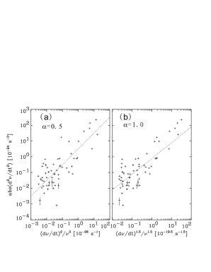
Figure 3: Correlations between $\ddot{\nu}$ and $(-\dot{\nu})^{1+\beta}/\nu^{3\beta}$ with $\alpha=0.5$ (panel (a)) and $\alpha=1.0$ (panel (b)) for young pulsars with $\tau_{\rm c}\leq 2\times 10^{6}$ yr and $\ddot{\nu}>0$. The dotted lines are the best-fit of $\ddot{\nu}=\eta(-\dot{\nu})^{1+\beta}/\nu^{3\beta}$. This figure is taken from Paper I.

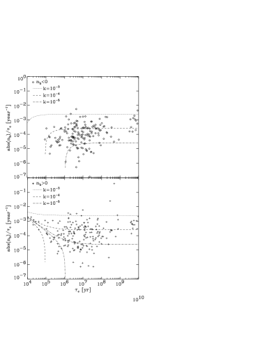
Figure 4: Correlation between $n_{\rm b}/\tau_{\rm c}$ and $\tau_{\rm c}$. The different curves show the analytically calculated model predictions using Equation (14) for different values of $k$. The figure is taken from Paper II.

In Figure 4 (taken from Paper II), we show the observed correlation between $n_{\rm b}/\tau_{\rm c}$ and $\tau_{\rm c}$, overplotted with the analytical results of Equation (14) with $C(t)=\pm 1$, $T=10$ yr and $k=10^{-3},\ 10^{-4}$ and $10^{-5}$, respectively. Once again, the analytical results agree with the data quite well.

We also performed Monte Carlo simulations for the distributions of reported data (H2010) in $\ddot{\nu}$-$\tau_{\rm c}$ and $n$-$\tau_{c}$ diagrams, as shown in Figure 5 (taken from Paper IV), respectively. The two dimensional K-S tests show that the distributions of two samples in each panel are remarkably consistent.

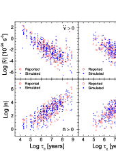
Figure 5: $\ddot{\nu}$-$\tau_{\rm c}$ and $n$-$\tau_{c}$ diagrams. The simulated data and reported data are represented with solid circles and open circles, respectively. The figure is taken from Paper IV.

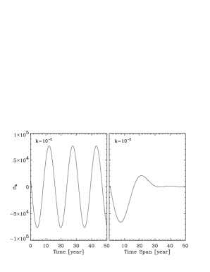
Figure 6: Left: “instantaneous” braking index $n_{\rm b}$ as a function of time. Right: “averaged” braking index $n_{\rm b}$ as a function of the time span of the fitting. $T=15$ yr is used in both cases. The figure is taken from Paper II.

4.2 The instantaneous and averaged values of $n_{\rm b}$

Equation (14) gives $n_{\rm b}$ as a function of $t$, i.e., the calculated $n_{\rm b}$ is in fact a function of time for a given pulsar, as shown in the left panel of Figure 6, in which the horizontal axis “Time” is the calendar time. We call $n_{\rm b}$ calculated this way the “instantaneous” braking index. However, in analyzing the observed timing data of a pulsar, one usually fits the data on TOAs over a certain time span to Equation (1), where $\Phi(t)$ is the phase of TOA of the observed pulses, and $\Phi_{0}$, $\nu_{0}$, $\dot{\nu}_{0}$ and $\ddot{\nu}_{0}$ are the values of these parameters at $t_{0}$, to be determined from the fitting. $n_{\rm b}$ calculated from $\nu_{0}$, $\dot{\nu}_{0}$ and $\ddot{\nu}_{0}$ is thus not exactly the same as the “instantaneous” braking index. We call $n_{\rm b}$ calculated this way over a certain time span the “averaged” braking index.

In the right panel of Figure 6, we show the simulated result for the “averaged” braking index as a function of time span. It can be seen that the “averaged” $n_{\rm b}$ is close to the “instantaneous” one when the time span is shorter than $T$, which is the oscillation period of the magnetic fields. The close match between our model predicted “instantaneous” $n_{\rm b}$ and the “averaged” $n_{\rm b}$, as shown in Figure 4, suggests that the time spans used in the H2010 sample are usually smaller than $T$.

For some pulsars the observation history may be longer than $T$ and one can thus test the prediction of Figure 6 with the existing data. In doing so, we can also obtain both $f$ and $T$ for a pulsar, thus allowing a direct test of our model for a single pulsar. We can in principle then include the model of magnetic field evolution for each pulsar in modeling its long term timing data, in order to remove the red noise in its timing residuals, which may potentially be the limiting factor to the sensitivity in detecting gravitational waves with pulsars.

5 A phenomenological model for glitches

In this section, we describe the phenomenological spin-down model for the glitch and slow glitch recoveries (see Xie & Zhang 2013; hereafter Paper III). We found that Equation (8) can be modified slightly to describe a glitch event,

$$\dot{\nu}\nu^{-3}=-H_{0}G(t),$$ (16)

where $H_{0}=\frac{8\pi^{2}(BR^{3}\sin\chi)^{2}}{3c^{3}I}=1/2\tau_{\rm c}\nu_{0}^{2}$, $\tau_{\rm c}=-\nu/2\dot{\nu}$ is the characteristic age of a pulsar, and $G(t)$ represents very small changes in the effective strength of dipole magnetic field $B\sin\chi$ during a glitch recovery. In the following we assume $G(t)=1+\kappa e^{-\Delta t/\tau}$.

Integrating and solving Equation (16), we have

$$\nu(t)\approx\nu_{0}+\Delta\nu_{\rm d}e^{-\Delta t/\tau}.$$ (17)

The derivative of $\nu$ is

$$\dot{\nu}(t)\approx\dot{\nu}_{0}-\Delta\dot{\nu}_{\rm d}e^{-\Delta t/\tau}.$$ (18)

We know $\Delta t\sim\tau\sim 100~{}{\rm days}$ and $\kappa\ll 1$.

In Figure 7 (taken from Paper III), we show the simulations for the reported three slow glitches of B1822-09 over the 1995-2004 interval. We confirmed that the slow glitch behavior can be explained by our phenomenological model with $\kappa<0$. It is also clear that the instantaneous values of $\Delta\dot{\nu}$, which are obtained directly with the model with the parameters are given by the simulation, are much larger than the reported results in literature.

Yuan et al. (2010) reported a very large glitch occurred between 2005 August 26 and September 8 (MJDs 53608 and 53621), the largest known glitch ever observed, with a fractional frequency increase of $\Delta\nu/\nu\sim 20.5\times 10^{-6}$. In the left panels of Figure 8, we show the fits with one exponential term $G(t)=(1+\kappa\exp{(-\Delta t/\tau)})$ for a comparison with the “realistic” simulation of two terms below. We show the modeled glitch recovery with $G(t)=(1+\kappa_{1}\exp{(-\Delta t/\tau_{1})}+\kappa_{2}\exp{(-\Delta t/\tau_{2})})$ in the right panels of Figure 8. Clearly the simulated profiles of the two term fit matches the reported ones better than that of the one term fit. One can see that $|\Delta\dot{\nu}_{\rm I}|$ are also slightly larger than the reported $|\Delta\dot{\nu}_{\rm O}|$ for both the one-term fit and two-term fit.

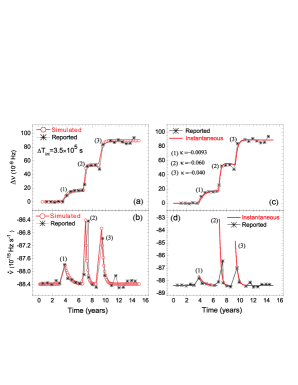
Figure 7: Slow glitches of Pulsar B1822–09. Observational results are taken from Shabanova (2005). Upper panels: variations of $\Delta\nu$ relative to the pre-glitch solution. Bottom panels: variations of $\dot{\nu}$. Left panels: comparison between the reported and simulated (both are also time-averaged) $\Delta\nu$ and $\dot{\nu}$. Right panels: comparison between the reported and restored (i.e. model-predicted) instantaneous $\Delta\nu$ and $\dot{\nu}$. The figure is taken for Paper III.

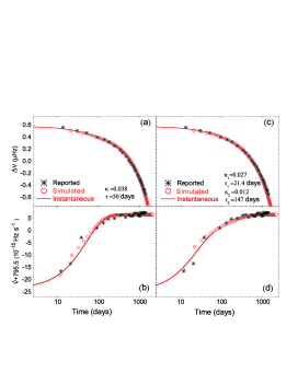
Figure 8: The giant glitch of Pulsar B2334+61. Observational results are taken from Yuan et al. 2010. Upper panels: variations of $\Delta\nu$. Bottom panels: variations of $\dot{\nu}$. The left and right panels represent for models with one and two decay components, respectively. The figure is taken for Paper III.

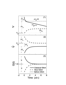
Figure 9: Schematic depictions of $\nu$, $\dot{\nu}$ and $G(t)$ for the slow and classical glitch recoveries. The pre-glitch tracks are represented by dotted line. The classical glitch recoveries are represented by solid lines. The slow glitches are represented by dashed lines.

We thus concluded that the classical and slow glitch recoveries can be well modeled by a simple function, $G(t)=1+\kappa\exp{(-\Delta t/\tau)}$, with positive or negative $\kappa$, respectively. Based on the results, we generalize the variations of $\nu$ and $\dot{\nu}$ for slow and classical glitch recoveries, as shown in Figure 9. The pre-glitch tracks are represented by dotted line. After the jump, the classical glitch recoveries (represented by solid line) generally have $\nu$ variation that tends to restore its initial values, and usually the restoration is composed by a exponential decay and a permanent linear decrease with slope $\Delta\dot{\nu}_{\rm p}$; however, for slow glitches (represented by dashed line), $\nu$ monotonically increases, as shown in panel (1). In panel (2), $\dot{\nu}$ of classical glitch recoveries that tends to restore its initial values, but cannot completely recover for $\Delta\dot{\nu}_{\rm p}\neq 0$; $\dot{\nu}$ of slow glitch recoveries almost completely recover to its initial value, corresponding to the increase of $\nu$.

The function, $G(t)=1+\kappa\exp{(-\Delta t/\tau)}$, with positive or negative $\kappa$, are shown in panel (3), respectively. However, it is should be noticed that the model only have two parameters, $\kappa$ and $\tau$, from which we can obtain $\Delta\nu_{\rm d}$ and $\Delta\dot{\nu}_{\rm d}$, but not $\Delta\nu_{\rm p}$ and $\Delta\dot{\nu}_{\rm p}$, which are not modelled. The expression of $\Delta\nu_{\rm p}$ and $\Delta\dot{\nu}_{\rm p}$ that relate to the initial jumps of $\nu_{0}$ and $\dot{\nu}_{0}$, are not given by the model, since the glitch relaxation processes are only considered here. It has been suggested that these non-recoverable jumps are the consequence of permanent dipole magnetic field increase during the glitch event (Lin and Zhang 2004). Nevertheless, we conclude that the major difference between slow glitch and classical glitch recoveries are that they show opposite trends with opposite signs of $\kappa$, in our phenomenological model.

Also as shown above, all the reported results of all pulsar glitches are systematically biased, and thus cannot be compared directly with theoretical models. In Paper III, we carried extensive simulations in examining all possible sources of biases due to imperfections both in observations, analysis methods, and the ways in reporting results in literature. We suggested some fitting procedures that can significantly reduce the biases for fitting the observed glitch recoveries and comparison with theoretical models.

6 Summary

We tested models of magnetic field evolution of NSs with the observed spin evolutions of individual pulsars and the statistical properties of their timing noise. In all models, the magnetic dipole radiation is assumed to dominate the instantaneous spin-down of pulsars; therefore, different models of their magnetic field evolution lead to different properties of their spin-down. We constructed a phenomenological model of the evolution of the magnetic fields of NSs, which is made of a long-term decay modulated by short-term oscillations. By comparising our model predictions with the precisely observed spin-down evolutions of some individual pulsars, we found that the Hall drift and Hall waves in the NS crusts are responsible for the long-term change and short-term quasi-periodical oscillations, respectively. We showed that the observed braking indices of the pulsars in the sample of H2010, which span over a range of more than 100 millions, can be completely reproduced with the model. We find that the “instantaneous” braking index of a pulsar may be different from the “averaged” braking index obtained from data. We also presented a phenomenological model for the recovery processes of classical and slow glitches, which is used to successfully model the observed slow and classical glitch events from pulsars B1822-09 and B2334+61, respectively. Significant biases are found for fitting glitch recovery, in the widely used fitting procedures and reported results in literature.

- [1] Blandford, R.D., & Romani, R.W.: 1988, MNRAS 234, 57P
- [2] Cumming, A., Arras, P., & Zweibel, E.,: ApJ 609, 999
- [3] Goldreich, P. & Reisenegger, A.: 1992, ApJ 395, 250
- [4] Lin, J. R., & Zhang, S. N. 2004, ApJL, 615, L133
- [5] Lorimer, D. R., & Kramer, M.: 2004, Handbook of Pulsar Astronomy (Cambridge University Press, Cambridge)
- [6] Lyne, A., Graham-Smith, F.: 2012, Pulsar Astronomy (Cambridge University Press, Cambridge)
- [7] Lyne, A., et al.: 2010, Science 329, 408
- [8] Hewish, A., et al.: 1968, Nature 217, 709
- [9] Hobbs, G., Lyne, A.G., & Kramer, M.: 2010, MNRAS 402, 1027 (H2010)
- [10] Manchester, R.N., & Taylor, J.H.: 1977, in Pulsars, ed. R. N. Manchester & J. H. Taylor (San Francisco, CA: W. H. Freeman), 281
- [11] Shabanova, T.V.: 2005, MNRAS 356, 1435
- [12] Xie, Y., & Zhang, S.-N.,: 2013, ApJ 778, 31 (Paper III)
- [13] Xie, Y., & Zhang, S.-N.,: arXiv:1307.6413 (Paper IV)
- [14] Xie, Y., & Zhang, S.-N.,: arXiv:1312.3049 (Paper V)
- [15] Yuan, J.P., et al.: 2010, ApJ 719, L111
- [16] Zhang, S.-N., & Xie, Y.: 2012, ApJ 757, 153 (Paper I)
- [17] Zhang, S.-N., & Xie, Y.: 2012, ApJ 761, 102 (Paper II)