Entropy production and fluctuation theorems for Langevin processes under continuous non-Markovian feedback control

Abstract

Continuous feedback control of Langevin processes may be non-Markovian due to a time lag between the measurement and the control action. We show that this requires to modify the basic relation between dissipation and time-reversal and to include a contribution arising from the non-causal character of the reverse process. We then propose a new definition of the quantity measuring the irreversibility of a path in a nonequilibrium stationary state, which can be also regarded as the trajectory-dependent total entropy production. This leads to an extension of the second law which takes a simple form in the long-time limit. As an illustration, we apply the general approach to linear systems which are both analytically tractable and experimentally relevant.

Introduction.– As famously illustrated by Maxwell’s demon thought experimentMNV2009 , entropy production (EP) in small thermodynamic systems can be reduced by the intervention of an external agent who possesses some information about the microstates. Recent years have seen a renewed interest for this idea due to the advances in the manipulation of mesoscopic objects and to a better understanding of the intimate relationship between EP and time asymmetry at the microscopic levelC1999 . The ultimate goal of these investigations is to develop a ‘thermodynamics of feedback’, relating information and dissipationCF2009 ; SU2012 .

With this goal in mind, we focus in this Letter on classical stochastic systems described by a Langevin dynamics and submitted to a continuous, non-Markovian feedback control. The non-Markovian character results from a time lag between the signal detection and the control action, which is an ubiquitous feature in biological systemsBR2000 and also plays an important role in many experimental setups (e.g. laser networksSGMF2013 ). Because of memory effects, the conventional approach of stochastic thermodynamicsJ2011 is not applicable to such systems, and even the basic identity (the so-called local detailed balance condition) which is at the heart of fluctuation relationsC1999 needs to be modified. Indeed, in order to relate the heat dissipated along an individual trajectory to the statistical weights of the trajectory and its time-reversal, causality must be artificially broken in the backward process, giving rise to a specific “Jacobian” contribution. Such effect went unnoticed in previous theoretical studies which mainly focused on discrete feedback protocols in which the controller acts at predetermined times. In this case, the reverse process is physically realizableTSUMS2010 , which is not possible when the feedback is applied continuously. This prompts us to propose a new definition of the fluctuating entropy production in a nonequilibrium stationary state (NESS), which in turn leads to a generalization of the second law. We illustrate this general approach by a detailed analytical and numerical study of linear systems. Note that the present study is restricted to the case of a deterministic (i.e. error-free) feedback control. Noise and measurement errors are known to reduce the achievable entropy reductionCF2009 .

Dissipation and time-reversal.– Without loss of generality, we consider the one-dimensional motion of a Brownian particle (or “system”) in contact with a heat bath in equilibrium at inverse temperature $\beta$ (Boltzmann constant is set to $1$ hereafter). The dynamics is described by a second-order Langevin equation with additive noise

$$m\ddot{x}+\gamma\dot{x}-F(x)-F_{fb}(t)=\xi(t)$$ (1)

where $m$ is a mass, $\gamma$ is a friction coefficient, $F(x)=-dU(x)/dx$ is a conservative force, and $\xi(t)$ is a delta-correlated white noise with variance $2\beta^{-1}\gamma$ (for simplicity, a memory-less friction is assumed, but the formalism can be generalized to a non-Markovian bath, as considered in previous studiesZBCK2005 ; OO2007 ; ABC2010 ). $F_{fb}(t)$ is the feedback control force determined by the measurement outcomes and which generally depends on the microscopic trajectory of the system in phase space up to time $t$. It may be for instance proportional to the position $x$ at time $t-\tau$, where $\tau$ is the delay (see Eq. (19) below), or to the velocity $\dot{x}$, as illustrated by Eq. (21) where $\tau$ is the relaxation time of the feedback mechanismMR2013 . This latter case is a non-Markovian generalization of the model studied in KQ2004 ; MR2012 which describes feedback cooling (or cold damping) experimental setupsPZ2012 .

In the normal operating regime of a continuous feedback control, the system settles into a NESS in which heat is permanently exchanged with the thermal environment (the stability of the NESS depends on the various parameters that specify the dynamics, e.g. the delay $\tau$). Within the framework of stochastic energeticsSeki1997 , the heat dissipated along an individual path ${\bf{\bf X}}\equiv\{x_{t},\dot{x}_{t}\}$ during the time interval $[-T,T]$ is then defined as

$$q[{\bf X},{\bf X}_{-}]\equiv\int_{-T}^{T}dt\>[\gamma\dot{x}_{t}-\sqrt{2\gamma\beta^{-1}}\xi_{t}]\>\dot{x}_{t}$$

$$=-\int_{-T}^{T}dt\>\Big{[}m\ddot{x}_{t}-F(x_{t})-F_{fb}[{\bf X},{\bf X_{-}}]\Big{]}\>\dot{x}_{t}\ ,$$ (2)

where ${\bf X_{-}}$ denotes the path for $t\leq-T$ (we now make explicit the fact that $F_{fb}(t)$ depends on both ${\bf X}$ and ${\bf X_{-}}$).

As in the case of Markov processes, we seek to relate $q[{\bf X},{\bf X}_{-}]$ to the time reversibility of the trajectories, so we consider the probability of observing ${\bf X}$ for a given initial state ${\bf x}_{i}\equiv(x_{-T},\dot{x}_{-T})$ and a given past trajectory ${\bf X_{-}}$note1 ; MRT2014 . This probability is determined by the noise history in the time interval $[-T,T]$ and given by

$${\cal P}[{\bf X}|{\bf x}_{i},{\bf X_{-}}]\propto\big{|}{\cal J}\big{|}\>e^{-\beta\int_{-T}^{T}dt\>{\cal S}[{\bf X},{\bf X_{-}}]}\ ,$$ (3)

where ${\cal S}[{\bf X},{\bf X_{-}}]$ is a generalized Onsager-Machlup action functionalOM1953 ,

$${\cal S}[{\bf X},{\bf X_{-}}] =\frac{1}{4\gamma}\Big{[}m\ddot{x}_{t}+\gamma\dot{x}_{t}-F(x_{t})-F_{fb}[{\bf X},{\bf X_{-}}]\Big{]}^{2}\ ,$$ (4)

and ${\cal J}$ is the Jacobian of the transformation $\xi(t)\rightarrow x(t)$ for $t\in[-T,T]$. Eq. (3) can be made rigorous by discretizing the Langevin dynamics, as done for instance in ABC2010 (in particular, there is no need to specify the interpretation of the stochastic calculus as long as $m\neq 0$). Due to causality, the Jacobian matrix is lower triangular, so that ${\cal J}$ is a path-independent positive quantity that can be included in the prefactornote2 .

We now replace the whole trajectory, including ${\bf X_{-}}$, by its time-reversed image $\{x^{\dagger}(t),\dot{x}^{\dagger}(t)\}=\{x(-t),-\dot{x}(-t)\}$ and consider the probability ${\cal P}[{\bf X^{\dagger}}|{\bf x}_{i}^{\dagger},{\bf X_{-}^{\dagger}}]$ of observing the reversed path ${\bf X^{\dagger}}$, given the path ${\bf X_{-}^{\dagger}}$ for $t\geq T$ and the initial state ${\bf x}_{i}^{\dagger}=(x_{T},-\dot{x}_{T})$. It is readily seen that in order to relate $q[{\bf X},{\bf X}_{-}]$ to the probabilities of ${\bf X}$ and ${\bf X}^{\dagger}$, one must define a new feedback force $\tilde{F}_{fb}$ such that $\tilde{F}_{fb}[{\bf X^{\dagger}},{\bf X_{-}^{\dagger}}]_{t\rightarrow-t}=F_{fb}[{\bf X},{\bf X_{-}}]$. (In the same vein, the driving protocol must be reversed in the case of a discrete feedback.) Consider for instance a time-delayed feedback $F_{fb}\propto x(t-\tau)$. Then $\tau$ must be changed into $-\tau$ in order to recover the original force. Similarly, in the case of an exponential memory kernel, $F_{fb}\propto\frac{1}{\tau}\int_{t_{0}}^{t}ds\>e^{-\frac{t-s}{\tau}}x(s)$, one must change $\tau$ into $-\tau$ and $t_{0}$ into $-t_{0}$. For a velocity-dependent feedback like in Eq. (21), one must also change $\gamma^{\prime}$ into $-\gamma^{\prime}$. More generally, such changes define a “conjugate” dynamics, hereafter denoted by the tilde symbol $(\sim)$. This dynamics is non-causal and does not correspond to any physical process, but the conditional probability

$$\tilde{\cal P}[{\bf X^{\dagger}}|{\bf x}_{i}^{\dagger},{\bf X_{-}^{\dagger}}]\propto\big{|}\tilde{\cal J}[{\bf X}]\big{|}\>e^{-\beta\int_{-T}^{T}dt\>\tilde{\cal S}[{\bf X^{\dagger}},{\bf X_{-}^{\dagger}}]}$$ (5)

with

$$\tilde{\cal S}[{\bf X^{\dagger}},{\bf X_{-}^{\dagger}}]=\frac{1}{4\gamma}\Big{[}m\ddot{x}_{t}-\gamma\dot{x}_{t}-F(x_{t})-\tilde{F}_{fb}[{\bf X^{\dagger}},{\bf X_{-}^{\dagger}}]_{t\rightarrow-t}\Big{]}^{2}$$ (6)

is a well-defined mathematical object. On the other hand, non-causality makes the Jacobian matrix no longer lower triangular and $\tilde{\cal J}[{\bf X}]$ is in general a nontrivial (positive) functional of the path (see Eq. (Entropy production and fluctuation theorems for Langevin processes under continuous non-Markovian feedback control) below). Taking the ratio of ${\cal P}[{\bf X}|{\bf x}_{i},{\bf X_{-}}]$ and $\tilde{\cal P}[{\bf X^{\dagger}}|{\bf x}_{i}^{\dagger},{\bf X_{-}^{\dagger}}]$ then leads to our first main result

$$\frac{{\cal P}[{\bf X}|{\bf x}_{i},{\bf X_{-}}]}{\tilde{\cal P}[{\bf X}^{\dagger}|{\bf x}_{i}^{\dagger},{\bf X}_{-}^{\dagger}]}=\frac{{\cal J}}{\tilde{\cal J}[{\bf X}]}\exp\big{\{}\beta\>q[{\bf X},{\bf X_{-}}]\big{\}}\ ,$$ (7)

which generalizes the familiar identity relating dissipation to time reversalC1999 . The two signatures of non-Markovianity are (i) the functional dependence on the past trajectory, and (ii) the presence of the ratio ${\cal J}/\tilde{\cal J}[{\bf X}]$ due to the non-causal character of the dynamics $\sim$.

Entropy production (EP).– As in the Markovian case, the left-hand side of Eq. (7) may be combined with normalized distributions ${\cal P}_{st}[{\bf x}_{i},{\bf X_{-}}]$ and ${\cal P}_{st}[{\bf x}_{i}^{\dagger},{\bf X}_{-}^{\dagger}]$ in order to define unconditional path weights. We thus introduce the quantity $R[{\bf X},{\bf X_{-}}]\equiv\Delta s_{m}[{\bf X},{\bf X_{-}}]-\ln\tilde{\cal J}[{\bf X}]/{\cal J}+\ln{\cal P}_{st}[{\bf x}_{i},{\bf X_{-}}]/{\cal P}_{st}[{\bf x}_{i}^{\dagger},{\bf X}_{-}^{\dagger}]$, where $\Delta s_{m}[{\bf X},{\bf X_{-}}]\equiv\beta q[{\bf X},{\bf X_{-}}]$ is the change in the entropy of the medium. By construction, $R[{\bf X},{\bf X_{-}}]$ satisfies the integral fluctuation theorem (IFT)

$$\langle e^{-R[{\bf X},{\bf X_{-}}]}\rangle_{st}=1$$ (8)

where $\langle...\rangle_{st}$ denotes an average over all paths ${\bf X}$ and ${\bf X_{-}}$ weighted by the stationary probability ${\cal P}_{st}[{\bf X},{\bf X_{-}}]$. It is worth noting that $R[{\bf X},{\bf X_{-}}]$ can also be expressed as

$$R[{\bf X},{\bf X_{-}}] =\Delta s_{tot}[{\bf X},{\bf X_{-}}]-\ln\tilde{\cal J}[{\bf X}]/{\cal J}$$

$$-\Delta{\cal I}[{\bf X}_{-},{\bf x}_{i},{\bf x}_{i}^{\dagger}]+\ln{\cal P}_{st}[{\bf X_{-}}]/{\cal P}_{st}[{\bf X}_{-}^{\dagger}]$$ (9)

where $\Delta s_{tot}[{\bf X},{\bf X_{-}}]\equiv\Delta s_{m}[{\bf X},{\bf X_{-}}]+\ln p_{st}({\bf x}_{i})/p_{st}({\bf x}_{i}^{\dagger})$ is a “Markovian-like” contributionJ2011 and $\Delta{\cal I}={\cal I}[{\bf x}_{i}^{\dagger}:{\bf X}_{-}^{\dagger}]-{\cal I}[{\bf x}_{i}:{\bf X}_{-}]=\ln{\cal P}_{st}[{\bf x}_{i}^{\dagger}|{\bf X_{-}}^{\dagger}]/p_{st}({\bf x}_{i}^{\dagger})-\ln{\cal P}_{st}[{\bf x}_{i}|{\bf X_{-}}]/p_{st}({\bf x}_{i})$ describes memory effects not contained in $\Delta s_{tot}[{\bf X},{\bf X_{-}}]$ (here, ${\cal I}$ is a fluctuating mutual information). A drawback, however, is that $R[{\bf X},{\bf X_{-}}]$ do not vanish when the feedback control is switched off and the system goes back to equilibrium (whereas $\Delta s_{tot}=0$). This problem is cured by considering the coarse-grained functional $R_{cg}[{\bf X}]=-\ln\int{\cal D}{\bf X}_{-}{\cal P}[{\bf X}_{-}|{\bf X}]\>e^{-R[{\bf X},{\bf X_{-}}]}$ which, from the definition of $R[{\bf X},{\bf X_{-}}]$, simply reads

$$R_{cg}[{\bf X}]\equiv\ln\frac{{\cal P}_{st}[{\bf X}]}{\tilde{\cal P}_{st}[{\bf X}^{\dagger}]}\ ,$$ (10)

where $\tilde{\cal P}_{st}[{\bf X}^{\dagger}]\equiv\int{\cal D}{\bf X}_{-}\tilde{\cal P}[{\bf X}^{\dagger}|{\bf x}_{i}^{\dagger},{{\bf X}}_{-}^{\dagger}]{\cal P}_{st}[{\bf x}_{i}^{\dagger},{{\bf X}}_{-}^{\dagger}]$note3 . By construction $R_{cg}[{\bf X}]$ obeys the IFT, and its average

$$\langle R_{cg}[{\bf X}]\rangle_{st}=\int{\cal D}{\bf X}\>{\cal P}_{st}[{\bf X}]\ln\frac{{\cal P}_{st}[{\bf X}]}{\tilde{\cal P}_{st}[{\bf X}^{\dagger}]}$$ (11)

is the Kullback-Leibler divergence $D({\cal P}_{st}||\tilde{\cal P}_{st})$ between the distributions ${\cal P}_{st}$ and $\tilde{\cal P}_{st}$. This quantity is always non-negative, which suggests that $R_{cg}[{\bf X}]$ properly describes the overall EP along the trajectory ${\bf X}$ as a measure of the irreversibility of the non-Markovian stationary process. In particular, $R_{cg}[{\bf X}]$ does not vanish when ${\cal P}_{st}[{\bf X}]={\cal P}_{st}[{\bf X}^{\dagger}]$, which occurs when all forces are linear (see below).

Asymptotic relations.– $R_{cg}[{\bf X}]$, however, is a complicated functional of the path (see MRT2014 for explicit calculations). On the other hand, its average has a simple expression when the observation time becomes much larger than the time constant characterizing the non-Markovian feedback (we here assume that the correlation to the past is finite or decreases rapidly with time, e.g. exponentially). The dependence on the past trajectory can then be neglected, as well as the “border” terms which are non extensive in time. This leads to the asymptotic equality

$$\langle R_{cg}[{\bf X}]\rangle_{st}\sim\langle\Delta s_{m}[{\bf X}]\rangle_{st}-\langle\ln\frac{\tilde{\cal J}[{\bf X}]}{{\cal J}}\rangle_{st}\ ,$$ (12)

which can be rewritten as $\dot{R}_{cg}=\dot{S}_{m}-\dot{S}_{{\cal J}}$ by defining the rates $\dot{R}_{cg}=\lim_{T\rightarrow\infty}\frac{1}{2T}\langle R_{cg}[{\bf X}]\rangle_{st}$, $\dot{S}_{m}=\frac{1}{2T}\langle s_{m}[{\bf X}]\rangle_{st}$ and $\dot{S}_{{\cal J}}=\lim_{T\rightarrow\infty}\frac{1}{2T}\langle\ln\tilde{\cal J}[{\bf X}]/{\cal J}\rangle_{st}$. Since $\langle R_{cg}[{\bf X}]\rangle_{st}$ is non-negative, Eq. (12) implies that

$$\dot{S}_{m}\geq\dot{S}_{{\cal J}}\ ,$$ (13)

which may be regarded as the generalized second law for the feedback controlled system. This is the central result of this Letter. The contribution $\dot{S}_{{\cal J}}$ represents the entropic cost of the feedback control and can be either negative or positive. It may be interpreted as a phase space ‘contraction’ or ‘expansion’ induced by the non-standard time-reversal transformation that leads to Eq. (7) (see also the comment below after Eq. (20)).

In addition to the inequality (13), we conjecture the following asymptotic integral fluctuation relation

$$\lim_{T\rightarrow\infty}\frac{1}{2T}\ln\langle e^{-\big{(}\Delta s_{tot}[{\bf X},{\bf X}_{-}]-\ln\frac{\tilde{\cal J}[{\bf X}]}{{\cal J}}\big{)}}\rangle_{st}=0$$ (14)

which is strongly supported by analyticalMRT2014 and numerical calculations (see Figs. 1 and 2). (Note that Eq. (14) involves $\Delta s_{tot}$ and not $\Delta s_{m}$. The latter displays strong fluctuations which are stabilized by the border term.)

Expression of the Jacobian. The Jacobian $\tilde{\cal J}[{\bf X}]$ thus plays a central role as the footprint of non-Markovianity and we devote the rest of this Letter to its calculation. The starting point is the operator representation of the conjugate, non-causal Langevin equation. Generalizing the analysis of OO2007 ; ABC2010 , one easily finds that $\tilde{\cal J}[{\bf X}]$ can be formally expressed as

$$\tilde{\cal J}[{\bf X}] ={\cal J}\exp\mbox{Tr}\ln[\delta_{t-t^{\prime}}-\tilde{M}_{tt^{\prime}}]$$

$$={\cal J}\exp-\sum_{n=1}^{\infty}\frac{1}{n}\int_{-T}^{T}dt\>\Big{\{}\underbrace{\tilde{M}\circ\tilde{M}\circ...\tilde{M}}_{n\>\mbox{times}}\Big{\}}_{tt}\$$ (15)

where the operator $\tilde{M}(t,t^{\prime})$ is defined by

$$\tilde{M}(t,t^{\prime})=\{G\circ\tilde{F}^{\prime}_{tot}\}_{tt^{\prime}}\equiv\int_{-T}^{T}dt^{\prime\prime}\>G(t-t^{\prime\prime})\tilde{F}^{\prime}_{tot}(t^{\prime\prime},t^{\prime})\ .$$ (16)

$G(t)$ is the Green function for the inertial and dissipative terms in the Langevin equation, and $\tilde{F}_{tot}^{{}^{\prime}}(t,t^{\prime})\equiv\delta\big{[}F(x(t))+\tilde{F}_{fb}[{\bf X},{\bf X}_{-}]\big{]}/\delta x(t^{\prime})$. In the white noise limit, one simply has $G(t)=\gamma^{-1}[1-e^{-\gamma t/m}]\Theta(t)$, where $\Theta(t)$ is the Heaviside step functionABC2010 .

Application to linear Langevin processes.– To be more specific, let us now consider the case of a harmonic oscillator submitted to a linear feedback control, which is relevant to many practical applications. Since we assume that the noise in Eq. (1) is white and Gaussian, all probabilities are Gaussian in the steady state and thus ${\cal P}[{\bf X}^{\dagger}]={\cal P}[{\bf X}]$. As already stressed, this implies that the quantity $\langle\ln{\cal P}[{\bf X}]/{\cal P}[{\bf X}^{\dagger}]\rangle_{st}$ which is commonly regarded as a measure of irreversibility (even for non-Markovian processesGPVdB2008 ; RP2012 ; DE2013 ) is a misleading indicator, in contrast with the quantity $R_{cg}[{\bf X}]$ introduced above.

The crucial simplification due to linearity is that the functional derivative $\tilde{F}^{\prime}_{fb}(t,t^{\prime})$ and thus $\tilde{\cal J}$ become path-independent. In what follows, we only consider the behavior for $T\rightarrow\infty$ and defer a more extensive analysis to MRT2014 . The operation $\circ$ in Eqs. (Entropy production and fluctuation theorems for Langevin processes under continuous non-Markovian feedback control)-(16) is then a convolution and $\tilde{M}(t,t^{\prime})$ becomes a function of $t-t^{\prime}$. This implies that $\ln\tilde{\cal J}/{\cal J}$ is proportional to $2T$, the duration of the trajectory, and the asymptotic rate $\dot{S}_{{\cal J}}=\lim_{T\rightarrow\infty}\frac{1}{2T}\ln\tilde{\cal J}/{\cal J}$ is obtained by Laplace transforming Eq. (Entropy production and fluctuation theorems for Langevin processes under continuous non-Markovian feedback control),

$$\dot{S}_{{\cal J}} =\frac{1}{2\pi i}\int_{c-i\infty}^{c+i\infty}ds\>\ln[1-\tilde{M}(s)]$$

$$=-\frac{1}{2\pi i}\sum_{n=1}^{\infty}\frac{1}{n}\int_{c-i\infty}^{c+i\infty}ds\>[\tilde{M}(s)]^{n}$$ (17)

where $\tilde{M}(s)\equiv\int_{-\infty}^{\infty}dt\>\tilde{M}(t)e^{-st}$ and $s=c+i\omega$. This can be also expressed as

$$\dot{S}_{{\cal J}}=\frac{1}{2\pi i}\int_{c-i\infty}^{c+i\infty}ds\>\ln\frac{G(s)}{\tilde{\chi}(s)}$$ (18)

where $\tilde{\chi}(s)=[G(s)^{-1}-\tilde{F}_{tot}^{\prime}(s)]^{-1}=[ms^{2}+\gamma s-\tilde{F}_{tot}^{\prime}(s)]^{-1}$ is the Laplace transform of the response function $\tilde{\chi}(t)$ associated with the conjugate Langevin equation. Note that we use here the bilateral Laplace transform because $\tilde{\chi}(t)$ is non-zero for $t<0$. In general, the integral in Eq. (18) must be computed numerically by properly choosing the value of $c$ (see Supplemental Material).

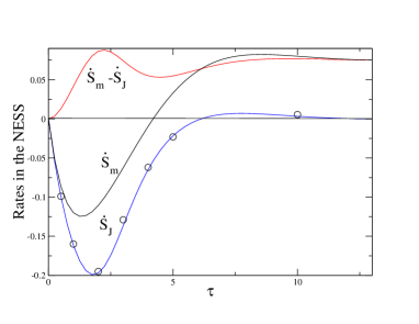
Figure 1: (Color on line) The rates $\dot{S}_{m}$, $\dot{S}_{{\cal J}}$ and $\dot{R}_{cg}=\dot{S}_{m}-\dot{S}_{{\cal J}}$ as a function of $\tau$ for the delay Langevin Eq. (19) with $m=1,\gamma=1,a=0.5$ and $b=-0.25$. The open circles are obtained from the equation $\dot{S}_{{\cal J}}\approx-\frac{1}{2T}\ln\langle e^{-\Delta s_{tot}}\rangle_{st}$ using $T=10$ and averaging over $10^{6}$ independent simulations of Eq. (19) with Heun’s method and a time step $\Delta t=10^{-3}$.

As a first application, we consider the stochastic delay equation

$$m\ddot{x}(t)+\gamma\dot{x}(t)+ax(t)+bx(t-\tau)=\xi(t)$$ (19)

which arises in a variety of mechanical or biological systems (e.g. in neural networks involved in the control of movement, posture, and visionPFFBT2006 ) and has been considered previously in the overdamped limit $m=0$MIK2009 ; JXH2011 (see the related discussion in MRT2014 ). When $m\neq 0$, the system settles into a NESS which is stable in a certain region of the parameter space and is characterized by an effective kinetic temperature $T_{k}\equiv m\langle\dot{x}^{2}\rangle_{st}$MRT2014 . Then $\dot{S}_{m}=\frac{\gamma}{m}(\beta T_{k}-1)$, which may become negative when the feedback is positive ($b<0$) and cools the system. This indicates that another entropic contribution must be taken into account in order to be consistent with the second law.

Focusing on the long-time limit, we first compute $\dot{S}_{{\cal J}}$ from expansion (Entropy production and fluctuation theorems for Langevin processes under continuous non-Markovian feedback control) which yields (see Supplemental Material)

$$\dot{S}_{{\cal J}}=\frac{b}{m}\tau-\frac{b\gamma}{2m^{2}}\tau^{2}+\frac{b(\gamma^{2}-am-4bm)}{6m^{3}}\tau^{3}+{\cal O}(\tau^{4})\ .$$ (20)

Interestingly, if one replaces $b\tau$ by $-\gamma^{\prime}$, the first-order term identifies with the so-called “entropy pumping” rate $\dot{S}_{pu}=-\gamma^{\prime}/m$ characteristic of a velocity-dependent feedback control KQ2004 ; MR2012 . One indeed recovers a force proportional to the velocity by expanding $x(t-\tau)$ at first order in $\tau$. In this sense, $\dot{S}_{{\cal J}}$ may be viewed as a generalization of $\dot{S}_{pu}$. To go beyond the small-$\tau$ expansion, Eq. (18) must be integrated numerically, using $\tilde{\chi}(s)=[ms^{2}+\gamma s+a+be^{s\tau}]^{-1}$.

As an illustration, we plot in Fig. 1 the rates $\dot{S}_{m}$, $\dot{S}_{{\cal J}}$, and $\dot{R}_{cg}=\dot{S}_{m}-\dot{S}_{{\cal J}}$ as a function of $\tau$ in the case of a positive feedback. One can see that $\dot{R}_{cg}$ is always positive, in agreement with the generalized second law, Eq. (13). The non-monotonous behavior of $\dot{S}_{m}$ is directly dictated by the behavior of $T_{k}$, which is not the case for $\dot{S}_{{\cal J}}$. Note also that $\dot{S}_{m}$ goes to a finite value for $\tau\rightarrow\infty$ whereas $\dot{S}_{{\cal J}}\rightarrow 0$. We also indicate in the figure some values of $\dot{S}_{{\cal J}}$ obtained by simulating the Langevin equation (19) and using Eq. (14) which takes the simple form $\lim_{T\rightarrow\infty}\frac{1}{2T}\ln\langle e^{-\Delta s_{tot}[{\bf X},{\bf X}_{-}]}\rangle_{st}=-\dot{S}_{{\cal J}}$ for a linear system. As can be seen, the agreement with the theoretical value is already very good with $T=10$.

As second application, we consider the equation

$$m\ddot{x}+\gamma\dot{x}+ax+\frac{\gamma^{\prime}}{\tau}\int_{-\infty}^{t}dt^{\prime}\>e^{-\frac{t-t^{\prime}}{\tau}}\dot{x}(t^{\prime})=\xi(t)$$ (21)

which may describe a feedback-cooled electromechanical oscillatorPZ2012 ; GRBC2009 . The molecular refrigerator model of KQ2004 ; MR2012 is recovered in the Markovian limit $\tau\rightarrow 0$. Since the system is linear, this also amounts to studying the coupled Markovian equationsMR2013

$$m\ddot{x}+\gamma\dot{x}+ax+\gamma^{\prime}y =\xi(t)$$

$$\dot{y}+\frac{1}{\tau}(y-\dot{x}) =\eta(t)$$ (22)

in the limit where the noise $\eta$ becomes negligible. More generally, such coupled equations are useful to investigate the role of coarse-graining and hidden degrees of freedom on fluctuation theoremsCPV2012 ; KN2013 ; IS2013 .

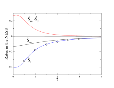
Figure 2: (Color on line) Same as Fig. 1 for the velocity-dependent feedback described by Eq. (21). The model parameters are $m=1,a=1,\gamma=0.2,\gamma^{\prime}=0.4$. Note that $\dot{S}_{{\cal J}}\rightarrow-\frac{\gamma^{\prime}}{m}$ for $\tau\rightarrow 0$.

For $\gamma^{\prime}>0$, heat permanently flows from the bath to the system in the steady state, with a rate given by Eq. (77) in MR2013 with $T^{\prime}=0$. This yields $\dot{S}_{m}=-(\gamma\gamma^{\prime})/(m\gamma_{eff})$ where $\gamma_{eff}=(\gamma+\gamma^{\prime})(1+\gamma\tau/m)+a\gamma\tau^{2}/m$. The conjugate dynamics is now defined by the changes $\tau\rightarrow-\tau$ and $\gamma^{\prime}\rightarrow-\gamma^{\prime}$, and the expansion (Entropy production and fluctuation theorems for Langevin processes under continuous non-Markovian feedback control) then yields

$$\dot{S}_{{\cal J}}=-\frac{\gamma^{\prime}}{m}+\frac{\gamma^{\prime}(\gamma-\gamma^{\prime})}{m^{2}}\tau+{\cal O}(\tau^{2})\ .$$ (23)

As it must be, the first term is just the entropy pumping contribution obtained in KQ2004 in the Markovian limit. This demonstrates that the present formalism is valid for both position- and velocity-dependent feedback control.

Some typical results for the rates as a function of $\tau$ are shown in Fig. 2. One again observes that the generalized second law (13) is obeyed and that Eq. (14) is in good agreement with the numerical simulations of the Langevin equation. In this model, both $\dot{S}_{m}$ and $\dot{S}_{{\cal J}}$ go to zero as $\tau\rightarrow\infty$.

Summary – By studying the nature of time-reversal breaking in the action functional of the path space measure, we have identified the unusual mathematical mechanism that contributes to the positivity of the entropy production in Langevin systems submitted to a continuous (position- or velocity-dependent) non-Markovian feedback control. In particular, the present formalism extends the framework of stochastic thermodynamics to the vast class of time-delayed diffusion processes. An important step further will be to include measurement noise. This will also clarify the relationship with previous approaches, in particular the abstract theoretical setup presented in SU2012 , which still remains elusive.

We are grateful to G. Tarjus for his help in the interpretation of the IFT. M.L.R. also acknowledges useful exchanges with S. Ito and T. Sagawa.

Supplemental Material: Computation of $\dot{S}_{\cal J}$ for linear systems

As indicated in the main text, the asymptotic rate $\dot{S}_{\cal J}$ is conveniently computed in linear systems by taking the bilateral Laplace transform of Eq. (15). We give here some more details about the calculation.

The starting point is Eq. (16) which defines $\tilde{M}(t)$ for $T\rightarrow\infty$ as the convolution

$$\tilde{M}(t)\equiv\int_{-\infty}^{\infty}dt^{\prime}\>G(t-t^{\prime})\tilde{F}_{tot}^{\prime}(t^{\prime}-t)\ .$$ (24)

This yields $\tilde{M}(s)\equiv\int_{-\infty}^{\infty}dt\>\tilde{M}(t)e^{-st}=G(s)\tilde{F}_{tot}^{\prime}(s)$ (with $s=c+i\omega$), and thus $\tilde{\chi}(s)\equiv G(s)[1-\tilde{M}(s)]^{-1}=[G(s)^{-1}-\tilde{F}_{tot}^{\prime}(s)]^{-1}$, where

$$G(s)=\frac{1}{\gamma}\int_{0}^{\infty}dt(1-e^{-\gamma t/m})e^{-st}=\frac{1}{ms(s+\gamma/m)}\ .$$ (25)

We first consider the model governed by the time-delayed Langevin equation (19). The conjugate dynamics is defined by the change $\tau\rightarrow-\tau$, so that $\tilde{F}^{\prime}_{tot}(t)=-a\delta(t)-b\delta(t+\tau)$. This yields

$$\tilde{M}(t) =-\frac{a}{\gamma}(1-e^{-\gamma t/m})\Theta(t)$$

$$-\frac{b}{\gamma}(1-e^{-\gamma(t+\tau)/m})\Theta(t+\tau)$$ (26)

and thus $\tilde{M}(s)=-[a+be^{s\tau}][ms(s+\gamma/m)]^{-1}$ with the region of convergence (ROC) defined by $c>0$. In order to compute the series expansion defined in the second line of Eq. (17), the integration contour is then closed to the left-hand side of the complex $s$-plane and the successive terms in the series are obtained by adding the residues at the two poles $s=0$ and $s=-\gamma/m$. After reorderingMRT2014 , this yields the series expansion in $\tau$ given by Eq. (20). On the other hand, choosing the value of $c$ for the contour integral in Eq. (18) is a more delicate issue which requires to determine the position of the poles of $\tilde{\chi}(s)=[ms^{2}+\gamma s+a+be^{s\tau}]^{-1}$. A careful analysis shows that $\tilde{\chi}(s)$ has two poles on the l.h.s. of the complex $s$-plane and an infinity of poles on the r.h.s., which is the signature of non-causality. One can showMRT2014 that the correct choice for the integration contour is $0<c<c_{1}^{+}$, where $c_{1}^{+}$ denotes the pole closest to the imaginary axis. The numerical integration of Eq. (18) is then in agreement with the series expansion (20) when the latter converges.

We next consider the model described by Eq. (21) in the main text. The conjugate dynamics is defined by the changes $\tau\rightarrow-\tau$ and $\gamma^{\prime}\rightarrow-\gamma^{\prime}$ so that $\tilde{F}^{\prime}_{tot}(t)=-[a+(\gamma^{\prime}/\tau)]\delta(t)+(\gamma^{\prime}/\tau^{2})e^{t/\tau}\Theta(-t)$ by partial integration of $\tilde{F}_{fb}(t)$. Hence

$$\tilde{M}(t) =\left[-\frac{a}{\gamma}(1-e^{-\gamma t/m})+\frac{\gamma^{\prime}/m}{1+\gamma\tau/m}e^{-\gamma t/m}\right]\Theta(t)$$

$$+\frac{\gamma^{\prime}/m}{1+\gamma\tau/m}e^{t/\tau}\Theta(-t),$$ (27)

and $\tilde{M}(s)=[a-(a\tau+\gamma^{\prime})s]/[ms(s+\gamma/m)(\tau s-1)]$ with the ROC defined by $0<c<1/\tau$. The expansion (23) is then obtained from Eq. (17) by closing the contour either to the l.h.s and adding the residues at $s=0$ and $s=-\gamma/m$ or to the r.h.s. and taking the residue at $s=1/\tau$. To perform the numerical integration in Eq. (18), one must consider the position of the poles of $\tilde{\chi}(s)=[\tau s-1][m\tau s^{3}+(\gamma\tau-m)s^{2}+(\gamma^{\prime}-\gamma+a\tau)s-a]^{-1}$. In particular, the situation depends on the sign of $\gamma^{\prime}-\gamma$, which is reminiscent of the behavior of the large deviation function for the entropy production studied in MR2012 .

References

- (1) K. Maruyama, F. Nori, and V. Vedral, Rev. Mod. Phys. 81, 1 (2009); H. Touchette and S. Lloyd, Physica A 331 140 (2004).
- (2) G. E. Crooks, J. Stat. Phys. 90, 1481 (1998); Phys. Rev. E 60, 2721 (1999); J. Kurchan, J. Phys. A 31, 3719 (1998); J. L. Lebowitz and H. Spohn, J. Stat. Phys. 95, 333 (1999); C. Maes and K. Netocný, J. Stat. Phys., 110, 269 (2003); P. Gaspard, J. Stat. Phys. 117, 599 (2004); U. Seifert, Phys. Rev. Lett. 95, 040602 (2005); A. Imparato and L. Peliti, Phys. Rev. E 74, 026106 (2006); R. Kawai, J. M. R. Parrondo, and C. Van den Broeck, Phys. Rev. Lett. 98, 080602 (2007); D. Andrieux et al., J. Stat. Mech. P01002 (2008).
- (3) F. J. Cao and M. Feito, Phys. Rev. E 79, 041118 (2009); T. Sagawa and M. Ueda, Phys. Rev. Lett. 104, 090602 (2010); J. M. Horowitz and S. Vaikuntanathan, Phys. Rev. E 82, 061120 (2010); Y. Fujitani and H. Suzuki, J. Phys. Soc. Jap. 79, 104003 (2010); M. Ponmurugan, Phys. Rev. E 82, 031129 (2010); J. M. Horowitz and J. M. R. Parrondo, Europhys. Lett. 95, 10005 (2011); D. Abreu and U. Seifert, Phys. Rev. Lett. 108, 030601 (2012); M. Esposito and G. Schaller, Euro. Phys. Lett. 99, 30003 (2012); D. Mandal and C. Jarzynski, PNAS 109, 11641 (2012).
- (4) T. Sagawa and M. Ueda, Phys. Rev. E 85, 021104 (2012).
- (5) See e.g. G. A. Bocharov and F. A. Rihan, J. Comp. and App. Math. 125, 183 (2000) and references therein.
- (6) M. C. Soriano, J. Garcia-Ojalvo, C. R. Mirasso, and I. Fischer, Rev. Mod. Phys. 85, 421 (2013).
- (7) For recent reviews and extensive references see C. Jarzynski, Annual Review of Condensed Matter Physics 2, 329 (2011), and U. Seifert, Rep. Prog. Phys. 75, 126001 (2012).
- (8) S. Toyabe et al., Nature Physics. 6, 988 (2010).
- (9) F. Zanponi, F. Bonetto, L. F. Cugliandolo, and J. Kurchan, J. Stat. Mech. P09013 (2005); T. Mai and A. Dhar, Phys. Rev. E 75, 061101 (2007); T. Speck and U. Seifert, J. Stat. Mech. L09002 (2007).
- (10) T. Ohkuma and T. Ohta, J. Stat. Mech. P10010 (2007).
- (11) C. Aron, G. Biroli, and L. F. Cugliandolo, J. Stat. Mech. P11018 (2010).
- (12) T. Munakata and M. L. Rosinberg, J. Stat. Mech. P06014 (2013).
- (13) K. H. Kim and H. Qian, Phys. Rev. Lett. 93, 120602 (2004); Phys. Rev. E 75, 022102 (2007).
- (14) T. Munakata and M. L. Rosinberg, J. Stat. Mech. P05010 (2012).
- (15) See M. Poot and H. S. J. van der Zant, Phys. Rep. 511, 273 (2012) and references therein.
- (16) K. Sekimoto, Stochastic Energetics, Lect. Notes Phys. 799 (Springer, Berlin Heidelberg 2010).
- (17) When the two trajectories and are contiguous (e.g., with ), the probability of observing is only conditioned by . However, it is technically convenient to keep the dependence on and introduce a Dirac delta function in the equations at a later stageMRT2014 .
- (18) T. Munakata, M. L. Rosinberg, and G. Tarjus, in preparation.
- (19) L. Onsager and S. Machlup, Phys. Rev. 91, 1505 (1953).
- (20) As is well known, there is an additional path-dependent contribution if one sets from the outset, see e.g. V. Y. Chernyak, M. Chertkov, and C. Jarzynski, J. Stat. Mech. P08001 (2006).
- (21) This must regarded as a shorthand notation since is not a stationary probability associated with a real process.
- (22) A. Gomez-Marin, J. M. Parrondo, and C. Van den Broeck, Phys. Rev. E. 78, 011107 (2008).
- (23) E. Roldán and J. M. R. Parrondo, Phys. Rev. E 85, 031129 (2012).
- (24) G. Diana and M. Esposito, arXiv:1307.4728 (2013) (to appear in J. Stat. Mech).
- (25) K. Patanarapeelert et al., Phys. Rev. E 73, 021901 (2006).
- (26) T. Munakata, S. Iwama, and M. Kimizuka, Phys. Rev. 79, 031104 (2009).
- (27) H. Jiang, T. Xiao, and Z. Hou, Phys. Rev. E 83, 061144 (2011).
- (28) P. De Gregorio, L. Rondoni, M. Bonaldi, and L. Conti, J. Stat. Mech. P10016 (2009).
- (29) A. Crisanti, A. Pusigli, and D. Villamaina, Phys. Rev. E 85, 061127 (2012).
- (30) K. Kawaguchi and Y. Nakayama, Phys Rev E 88, 022147 (2013).
- (31) S. Ito and T. Sagawa, Phys. Rev. Lett. 111, 180603 (2013).