Abstract

We consider a scenario where supersymmetry is broken at a high energy scale, out of reach of the LHC, but leaves a few fermionic states at the TeV scale. The particle content of the low-energy effective theory is similar to that of Split Supersymmetry. However, the gauginos and higgsinos are replaced by fermions carrying the same quantum numbers but having different couplings, which we call fake gauginos and fake higgsinos. We study the prediction for the light-Higgs mass in this Fake Split-SUSY Model (FSSM). We find that, in contrast to Split or High-Scale Supersymmetry, a 126 GeV Higgs boson is easily obtained even for arbitrarily high values of the supersymmetry scale $M_{\scriptscriptstyle S}$. For $M_{\scriptscriptstyle S}\gtrsim 10^{8}$ GeV, the Higgs mass is almost independent of the supersymmetry scale and the stop mixing parameter, while the observed value is achieved for $\tan{\beta}$ between $1.3$ and $1.8$ depending on the gluino mass.

1 Introduction

The LHC experiments have completed the discovery of all of the particles predicted by the Standard Model (SM). The uncovering of the last building block, the Higgs boson [1, 2], opens the way for a more precise experimental investigation of the electroweak sector. Of particular interest is understanding the possible role of supersymmetry.

Supersymmetry (SUSY) can find diverse motivations. From a lower-energy point of view, (i) it eases the problem of the hierarchy of the gauge-symmetry-breaking scale versus the Planck scale; (ii) it provides candidates for dark matter; (iii) it allows unification of gauge couplings and even predicts it within the Minimal Supersymmetric Standard Model (MSSM). On the other hand, supersymmetry can be motivated as an essential ingredient of the ultraviolet (UV) theory, having String Theory in mind. In the latter framework, there is no obvious reason to expect supersymmetry to be broken at a particular scale, which is usually requested to be much below the fundamental one. The original motivations of low-energy supersymmetry might then be questioned. In fact, the Split-Supersymmetry model [3, 4, 5] abandons (i) among the motivations of supersymmetry, while retaining (ii) and (iii). The idea of Split SUSY is to consider an MSSM content with a split spectrum. All scalars but the lightest Higgs are taken to be very massive, well above any energy accessible at near-future colliders, while the gauginos and the higgsinos remain light, with masses protected by an approximate $R$-symmetry.

It is important to emphasise that, even if supersymmetry is broken at an arbitrarily high scale $M_{\scriptscriptstyle S}$, its presence still has implications at low energy for the Higgs mass. Indeed, in supersymmetric models the value of the Higgs quartic coupling is fixed once the model content and superpotential couplings are given. This provides a boundary condition at $M_{\scriptscriptstyle S}$ for the renormalisation group (RG) evolution down to the weak scale to predict the value of the Higgs mass. As a result, in the Split-SUSY model the prediction for the light-Higgs mass can be in agreement with the measured value of about $126$ GeV only for values of $M_{\scriptscriptstyle S}$ not exceeding about $10^{9}$ GeV (see for example refs [6, 7]).

In this paper we consider a new scenario. In the spirit of Split SUSY, we assume that fine-tuning is responsible for the presence of a light Higgs. A first difference is that our UV model is not the MSSM but it is extended by additional states in the adjoint representation of the SM gauge group, as in ref. [8]. Such a field content has been discussed in the so-called Split Extended SUSY [9, 10] (see also [11, 12] for related work), where it was assumed that the additional gaugino-like and higgsino-like states arise as partners of the SM gauge bosons under an extended supersymmetry, and different hierarchies between the Dirac and Majorana masses have been considered in ref. [13]. Furthermore, in related work a similar scenario to ours was recently presented in [14].

A fundamental difference between our scenario and the usual Split SUSY or the closely related models mentioned above is that $R$-symmetry is strongly broken and does not protect the gauginos from obtaining masses comparable to the scalar ones [14]. In the simplest realisation presented here, in order to keep the extra states light, we endow them with charges under a new $U(1)_{\scriptscriptstyle F}$ symmetry. An $N=2$ supersymmetry origin of the new states [9, 10] raises then the difficulty of embedding $U(1)_{\scriptscriptstyle F}$ in an $R$-symmetry and will not be discussed here.

For $M_{\scriptscriptstyle S}$ lower than the MSSM GUT scale $M_{\rm{\scriptscriptstyle GUT}}\approx 2\!\times\!10^{16}$ GeV, the achievement of unification requires additional superfields which restore convergence of the three SM gauge couplings. This set of extra states can be chosen to be the ones that are required for unification of gauge couplings in Dirac gaugino unified models [15], and can safely be assumed to appear only above $M_{\scriptscriptstyle S}$, not affecting the discussion in this work: the properties of our model are fixed at $M_{\scriptscriptstyle S}$ and, as we shall establish, any corrections that we cannot determine are tiny.

Below the supersymmetry scale $M_{\scriptscriptstyle S}$, the field content of the model is the same as in the usual Split SUSY, but the gauginos are replaced by very weakly coupled fermions in the adjoint representation that we call “fake gauginos”, and the higgsinos are replaced by weakly coupled fermion doublets that we call “fake higgsinos”. At the TeV scale the model looks like Split SUSY with fake gauginos and higgsinos, hence the name of Fake Split-SUSY Model (FSSM). As we will show, a remarkable consequence of the different couplings of the fake gauginos and higgsinos to the Higgs boson, compared to the usual gauginos and higgsinos, is that a prediction for the Higgs mass compatible with the observed value can be obtained for arbitrarily high values of $M_{\scriptscriptstyle S}$.

The plan of the paper is as follows. In section 2, we describe the field content of the Fake Split-SUSY Model and a possible realisation using a broken additional $U(1)_{\scriptscriptstyle F}$ symmetry. The latter will be at the origin of the desired hierarchy between different couplings and mass parameters. We explain how the effective field theory of the FSSM compares with the usual Split SUSY. Section 3 briefly discusses the collider and cosmological constraints. Section 4 presents the predictions of the model for the Higgs mass. The assumptions, inputs and approximations used in the computation are described in section 4.1, while numerical results are presented in section 4.2. We also provide a comparison with the cases of Split SUSY and High-Scale SUSY, showing the improvement for fitting the experimental value of the Higgs mass for arbitrarily high values of the supersymmetry scale $M_{\scriptscriptstyle S}$. Our main results, and open questions requiring further investigation, are summarised in the conclusions. Finally, the two-loop renormalisation group equations (RGEs) for the mass parameters of Split SUSY are given in an appendix.

2 The Fake Split-Supersymmetry Model

2.1 The model at the SUSY scale

At the high SUSY scale $M_{\scriptscriptstyle S}$, we extend the MSSM by additional chiral superfields and a $U(1)_{\scriptscriptstyle F}$ symmetry. There are three sets of additional states: 

1. Fake gauginos (henceforth, F-gauginos) are fermions $\chi_{\Sigma}$ in the adjoint representation of each gauge group, which sit in a chiral multiplet $\mathbf{\Sigma}$ having scalar component $\Sigma$. These consist of: a singlet $\mathbf{S}=S+\sqrt{2}\theta\chi_{S}+\ldots$ ; an $SU(2)$ triplet $\mathbf{T}=\sum_{a}\mathbf{T}^{a}\,\sigma^{a}/2$, where $\mathbf{T}^{a}=T^{a}+\sqrt{2}\theta\chi_{T}^{a}+\ldots$ and $\sigma^{a}$ are the three Pauli matrices; an $SU(3)$ octet $\mathbf{O}=\sum_{a}\mathbf{O}^{a}\,\lambda^{a}/2$, where $\mathbf{O}^{a}=O^{a}+\sqrt{2}\theta\chi_{O}^{a}+\ldots$ and $\lambda^{a}$ are the eight Gell-Mann matrices.

2. Higgs-like $SU(2)_{W}$ doublets $\mathbf{H_{u}^{\prime}}$ and $\mathbf{H_{d}^{\prime}}$ (henceforth, F-Higgs doublets) with fermions appearing as fake higgsinos (henceforth, F-higgsinos).

3. Two pairs of vector-like electron superfields (i.e. two pairs of superfields with charges $\pm 1$ under $U(1)_{Y}$) with a supersymmetric mass $M_{\scriptscriptstyle S}$. For $M_{\scriptscriptstyle S}\lesssim M_{\rm{\scriptscriptstyle GUT}}$ these fields restore the possibility of gauge coupling unification, because they equalise the shifts in the one-loop beta functions at $M_{\scriptscriptstyle S}$ of all of the gauge groups relative to the MSSM [15].

In contrast to the usual Split-SUSY case – and also in contrast to the usual Dirac gaugino case – we do not preserve an $R$-symmetry. This means that the gauginos have masses at $M_{\scriptscriptstyle S}$, moreover the higgsino mass is not protected, thus a $\mu$ term of order $M_{\scriptscriptstyle S}$ will be generated for the higgsinos.

However, we introduce an approximate $U(1)_{\scriptscriptstyle F}$ symmetry under which all the adjoint superfields and the F-Higgs fields $\mathbf{H_{u}^{\prime}}$ and $\mathbf{H_{d}^{\prime}}$ have the same charge. The breaking of this symmetry is determined by a small parameter $\varepsilon$ which may correspond to the expectation value of some charged field divided by the fundamental mass scale of the theory (at which Yukawa couplings are generated); this reasoning is familiar from flavour models. We can write the superpotential of the Higgs sector of the theory schematically as

$$W = \mu_{0}\,\mathbf{H_{u}\cdot H_{d}}+Y_{u}\,\mathbf{U^{c}\,Q\cdot H_{u}}-Y_{d}\,\mathbf{D^{c}\,Q\cdot H_{d}}-Y_{e}\,\mathbf{E^{c}\,L\cdot H_{d}}$$ (2.1)

$$+ \varepsilon\,\left(\hat{\mu}^{\prime}_{d}\,\mathbf{H_{u}\cdot H_{d}^{\prime}}+\hat{\mu}^{\prime}_{u}\,\mathbf{H_{u}^{\prime}\cdot H_{d}}+\hat{Y}_{u}^{\prime}\,\mathbf{U^{c}\,Q\cdot H_{u}^{\prime}}-\hat{Y}_{d}^{\prime}\,\mathbf{D^{c}\,Q\cdot H_{d}^{\prime}}-\hat{Y}_{e}^{\prime}\,\mathbf{E^{c}\,L\cdot H_{d}^{\prime}}\right)$$

$$+ \varepsilon\,\left(\hat{\lambda}_{S}\,\mathbf{S\,H_{u}\cdot H_{d}}+2\,\hat{\lambda}_{T}\,\mathbf{H_{d}\!\cdot\!T\,H_{u}}\right)$$

$$+ \varepsilon^{2}\,\left(\hat{\lambda}_{Sd}^{\prime}\,\mathbf{S\,H_{u}\cdot H_{d}^{\prime}}+\hat{\lambda}_{Su}^{\prime}\,\mathbf{S\,H_{u}^{\prime}\cdot H_{d}}+2\,\hat{\lambda}_{Tu}^{\prime}\,\mathbf{H_{d}\!\cdot\!T\,H_{u}^{\prime}}+2\,\hat{\lambda}_{Td}^{\prime}\,\mathbf{H_{d}^{\prime}\!\cdot\!T\,H_{u}}\right)$$

$$+ \varepsilon^{2}\,\hat{\mu}^{\prime\prime}\,\mathbf{H_{u}^{\prime}\cdot H_{d}^{\prime}}~{}+~{}\varepsilon^{2}\,\left[\frac{1}{2}\,\hat{M}_{S}\,\mathbf{S}^{2}+\hat{M}_{T}\,\textrm{Tr}(\mathbf{TT})+\hat{M}_{O}\,\textrm{Tr}(\mathbf{OO})\right]~{},$$

where we have neglected irrelevantly small terms of higher order in $\varepsilon$. Even if chosen to vanish in the supersymmetric theory, some parameters in eq. (2.1), such as the bilinear $\mu$ terms, obtain contributions when supersymmetry is broken. In order to keep track of the order of suppression, we have explicitly extracted the parametric dependence on $\varepsilon$ due to the $U(1)_{F}$ charges, such that all the mass parameters are of ${\cal O}(M_{\scriptscriptstyle S})$, and all the dimensionless couplings are either of order one or suppressed by loop factors.

Note that the “fake states” can appear as partners of the MSSM gauge bosons under an extended $N=2$ supersymmetry that is explicitly broken at the UV scale to $N=1$. The imprint of $N=2$ is the extension of the states in the gauge sector into gauge vector multiplets and Higgs hyper-multiplets which give rise to the fake gauginos and higgsinos when broken down to $N=1$. The quarks and leptons of the MSSM should be identified with purely $N=1$ states. The difficulty of such a scenario resides in making only parts of the $N=2$ multiplets charged under $U(1)_{\scriptscriptstyle F}$. It is then tempting to identify the $U(1)_{\scriptscriptstyle F}$ as part of the original $R$-symmetry. We will not pursue the discussion of such possibility here.

We will now review the spectrum of states resulting from eq. (2.1). The Higgs soft terms, and thence the Higgs mass matrix, can be written as a matrix in terms of the four-vector $v_{H}\equiv(H_{u},{H_{d}}^{*},H_{u}^{\prime},H_{d}^{\prime\,*})$

$$-\frac{1}{M_{\scriptscriptstyle S}^{2}}\mathcal{L}_{soft}~{}~{}\supset~{}~{} v_{H}^{\dagger}\left(\begin{array}[]{cccc}\mathcal{O}(1)&\mathcal{O}(1)&\mathcal{O}(\varepsilon)&\mathcal{O}(\varepsilon)\\ \mathcal{O}(1)&\mathcal{O}(1)&\mathcal{O}(\varepsilon)&\mathcal{O}(\varepsilon)\\ \mathcal{O}(\varepsilon)&\mathcal{O}(\varepsilon)&\mathcal{O}(1)&\mathcal{O}(\varepsilon^{2})\\ \mathcal{O}(\varepsilon)&\mathcal{O}(\varepsilon)&\mathcal{O}(\varepsilon^{2})&\mathcal{O}(1)\end{array}\right)v_{H}.$$ (2.6)

In the spirit of the Split-SUSY scenario, the weak scale is tuned to have its correct value, and the SM-like Higgs boson is a linear combination of the original Higgs and F-Higgs doublets:

$$H_{u}~{}\approx~{}\,\sin\beta\,H\,+\ldots~{},~{}~{}~{}\qquad H_{d}~{}\approx~{}\,\cos\beta\,i\sigma^{2}\,H^{*}\,+\dots~{},$$ (2.7)

$$H_{u}^{\prime}~{}\approx~{}\varepsilon\,H\,+\ldots~{},~{}~{}~{}\qquad H_{d}^{\prime}~{}\approx\varepsilon\,i\sigma^{2}\,H^{*}\,+\ldots~{},$$ (2.8)

where $\beta$ is a mixing angle and the ellipses stand for terms of higher order in $\varepsilon$. Due to the suppression of the mixing between the eigenstates by the $U(1)_{\scriptscriptstyle F}$ symmetry, this pattern is ensured. Note that, if we wanted to simplify the model, we could impose an additional unbroken symmetry under which the F-Higgs fields transform and are vector-like – for example, lepton number. In this way we would remove the mixing between the Higgs and F-Higgs fields. This is unimportant in what follows, since we are only interested in the light fields that remain.

Eqs (2.7) and (2.8) show that the SM-like Higgs boson is, to leading order in $\varepsilon$, a linear combination of the fields $H_{u}$ and $H_{d}$. Thus, the Yukawa couplings are unaffected compared to the usual Split-SUSY scenario. The original higgsinos are rendered heavy, while the light fermionic eigenstates consist of $\tilde{H}_{u}^{\prime}$ and $\tilde{H}_{d}^{\prime}\,$, with mass $\mu$ of ${\cal O}(\varepsilon^{2}M_{\scriptscriptstyle S})$ and an ${\cal O}(\varepsilon)$ mixing with the original higgsinos.

Since we are not preserving an $R$-symmetry, the original gaugino degrees of freedom will obtain masses of ${\cal O}(M_{\scriptscriptstyle S})$, and we will also generate $A$-terms of the same order (although there may be some hierarchy between them if supersymmetry breaking is gauge-mediated). On the other hand, since the adjoint fields transform under a (broken) $U(1)_{\scriptscriptstyle F}$ symmetry, Dirac mass terms for the gauginos and also masses for the adjoint fermions are generated by supersymmetry breaking, but they are suppressed by one and two powers of $\varepsilon$, respectively. We can write the masses for the gauginos $\lambda$ and the adjoint fermions $\chi$ as

$$-\Delta\mathcal{L}_{\rm gauginos}=M_{\scriptscriptstyle S}\,\bigg{[}\frac{1}{2}\,\lambda\lambda~{}+~{}\mathcal{O}(\varepsilon)\,\lambda\chi~{}+~{}\mathcal{O}(\varepsilon^{2})\chi\chi~{}+~{}{\rm h.c.}~{}\bigg{]}~{},$$ (2.9)

giving a gaugino/F-gaugino mass matrix

$$\mathcal{M}_{1/2}~{}\sim~{}M_{\scriptscriptstyle S}\,\begin{pmatrix}1&\mathcal{O}(\varepsilon)\\ \mathcal{O}(\varepsilon)&\mathcal{O}(\varepsilon^{2})\end{pmatrix}.$$ (2.10)

This leaves a heavy eigenstate of ${\cal O}(M_{\scriptscriptstyle S})$ and a light one of ${\cal O}(\varepsilon^{2}M_{\scriptscriptstyle S})$, where the light eigenstate is to leading order $\chi+\mathcal{O}(\varepsilon)\,\lambda$.

We will assume that the Dirac masses are generated by D-terms of similar order to the $R$-symmetry-violating F-terms. This means that $B$-type mass terms for the adjoint scalars are generated of ${\cal O}(\varepsilon^{2}M_{\scriptscriptstyle S}^{2})$ too. However, the usual supersymmetry-breaking masses for the adjoint scalars $S,T,O$ will not be suppressed, and therefore will be at the scale $M_{\scriptscriptstyle S}$:

$$-\Delta\mathcal{L}_{\rm adjoint\ scalars}=M_{\scriptscriptstyle S}^{2}\,\bigg{[}|\Sigma|^{2}+\mathcal{O}(\varepsilon^{2})(\frac{1}{2}\Sigma^{2}+\frac{1}{2}\Sigma^{*\,2})\bigg{]}~{}.$$ (2.11)

This is straightforward to see in the case of gravity mediation, and in the case of gauge mediation we see that the triplet/octet adjoint scalars acquire these masses – as the sfermions do – at two loops (while in this case the singlet scalar would have a mass at an intermediate scale, but couplings to all light fields suppressed). This resolves in a very straightforward way the problem, typical of Dirac gaugino models, of having tachyonic adjoints [16, 17, 18].

2.2 Below $M_{\scriptscriptstyle S}$, the FSSM

Below the supersymmetry scale $M_{\scriptscriptstyle S}$, we can integrate out all of the heavy states and find that the particle content of the theory appears exactly the same as in Split SUSY: this is why we call the scenario Fake Split SUSY. Above the electroweak scale, we have F-Binos $\tilde{B}^{\prime}$, F-Winos $\tilde{W}^{\prime}$ and F-gluinos $\tilde{g}^{\prime}$ with (Majorana) masses $m_{\tilde{\scriptscriptstyle B}^{\prime}}$, $m_{\tilde{\scriptscriptstyle W}^{\prime}}$ and $m_{\tilde{g}^{\prime}}$, respectively, and F-higgsinos $\tilde{H}_{u,d}^{\prime}$ with a Dirac mass $\mu$.

We can also determine the effective renormalisable couplings. The F-gauginos and F-higgsinos have their usual couplings to the gauge fields. The F-gluinos have only gauge interactions, whereas there are in principle renormalisable interactions between the Higgs, F-higgsinos and F-electroweakinos. The allowed interactions take the form

$${\cal L}_{\rm eff}\supset-\frac{H^{\dagger}}{\sqrt{2}}(\tilde{g}_{2u}\,\sigma^{a}\,\tilde{W^{\prime}}^{a}+\tilde{g}_{1u}\,\tilde{B}^{\prime})\ \tilde{H}_{u}^{\prime}-\frac{H^{T}i\sigma^{2}}{\sqrt{2}}(-\tilde{g}_{2d}\,\sigma^{a}\,\tilde{W^{\prime}}^{a}+\tilde{g}_{1d}\,\tilde{B}^{\prime})\ \tilde{H}_{d}^{\prime}~{}.$$ (2.12)

Since the gauge couplings of all the particles are the same as in the usual Split-SUSY case, the allowed couplings take the same form. However, the values differ greatly. The couplings in eq. (2.12) descend from the gauge current terms, given by

$${\cal L}_{\rm gauge\ current}\supset -\frac{H^{\dagger}_{u}}{\sqrt{2}}(g\,\sigma^{a}\lambda_{2}^{a}+g^{\prime}\,\lambda_{Y})\ \tilde{H}_{u}-\frac{H_{d}^{\dagger}}{\sqrt{2}}(g\,\sigma^{a}\lambda_{2}^{a}-g^{\prime}\,\lambda_{Y})\ \tilde{H}_{d}$$

$$-\frac{H^{\prime\,\dagger}_{u}}{\sqrt{2}}(g\,\sigma^{a}\lambda_{2}^{a}+g^{\prime}\,\lambda_{Y})\ \tilde{H}^{\prime}_{u}-\frac{H_{d}^{\prime\,\dagger}}{\sqrt{2}}(g\,\sigma^{a}\lambda_{2}^{a}-g^{\prime}\,\lambda_{Y})\ \tilde{H}_{d}^{\prime}~{},$$ (2.13)

where $\lambda_{2},\lambda_{Y}$ are the gauginos of $SU(2)$ and hypercharge in the high-energy theory, but there are also terms of the same form from the superpotential terms $\varepsilon\hat{\lambda}_{S,T}$, $\varepsilon^{2}\hat{\lambda}_{Su,d}^{\prime}$, $\varepsilon^{2}\hat{\lambda}_{Tu,d}^{\prime}$ involving the fields $\chi_{S}$ and $\chi_{T}$. When we integrate out the heavy fields, we then see that in our model the couplings are doubly suppressed:

$$\tilde{g}_{1u}\sim\tilde{g}_{1d}\sim\tilde{g}_{2u}\sim\tilde{g}_{2d}\sim\varepsilon^{2}.$$ (2.14)

We recall that, in the usual Split-SUSY case, we would have instead $\tilde{g}_{2u}=g\sin\beta$, $\tilde{g}_{2d}=g\cos\beta$, $\tilde{g}_{1u}=g^{\prime}\sin\beta$ and $\tilde{g}_{1d}=g^{\prime}\cos\beta$, where $\beta$ is the angle that rotates the Higgs doublets $H_{u}$ and $H_{d}$ into one light, SM-like doublet and a heavy one.

The remaining renormalisable coupling in the theory is the Higgs quartic coupling $\lambda$, which at tree level is determined by supersymmetry to be

$$\lambda~{}=~{}\frac{1}{4}\left(g^{2}+g^{\prime\,2}\right)\,\cos^{2}2\beta~{}+~{}{\cal O}(\varepsilon^{2})~{}.$$ (2.15)

The tree-level corrections at $\mathcal{O}(\varepsilon^{2})$ come from the superpotential couplings $\hat{\lambda}_{S}$ and $\hat{\lambda}_{T}$, and from the $\mathcal{O}(\varepsilon)$ mixing between the Higgs and F-Higgs fields. Additional $\mathcal{O}(1)$ contributions to this relation could arise if the SUSY model above $M_{\scriptscriptstyle S}$ included new, substantial superpotential (or D-term) interactions involving the SM-like Higgs, but this is not the case for the model described in section 2.1. There are, however, small loop-level corrections to eq. (2.15), which we will discuss in section 4.

The $\mathcal{O}(\varepsilon^{2})$ corrections to the $\tilde{g}_{(1,2)(u,d)}$ and $\lambda$ couplings are not determined from the low-energy theory and are thus unknown. However, in this study we focus on models where the set of F-gauginos and F-higgsinos lies in the TeV mass range, which corresponds to values of $\varepsilon$ of the order of

$$\varepsilon\sim\sqrt{\frac{{\rm TeV}}{M_{\scriptscriptstyle S}}}~{},$$ (2.16)

which gives a $\varepsilon^{2}$ ranging between $10^{-13}$ to $10^{-2}$ when $M_{\scriptscriptstyle S}$ goes from the highest GUT scale of $10^{16}$ GeV down to $100$ TeV, the lowest scale considered here. With such values of $\varepsilon$, we have verified that we can safely neglect the contribution of $\tilde{g}_{(1,2)(u,d)}$ to the running of the Higgs quartic coupling, and that the shift in the Higgs mass due to the tree-level corrections to $\lambda$ is less than $2$ GeV for $M_{\scriptscriptstyle S}>100$ TeV, falling to a negligibly small amount for $M_{\scriptscriptstyle S}>1000$ TeV.

2.2.1 Gauge coupling unification

One of the main features of the MSSM that is preserved by the split limit is the unification of gauge couplings. At the one-loop level, the running of gauge couplings in our model is the same as in Split SUSY because the Yukawa couplings only enter at two-loop level. However, we have verified that gauge-coupling unification is maintained at two loops in our model.

2.2.2 Mass matrices

From the discussion above we can then read off the mass matrices after electroweak symmetry breaking. In the basis $(\tilde{B}^{\prime},\tilde{W}^{\prime\,0},\tilde{H^{\prime}_{d}}^{0},\tilde{H^{\prime}_{u}}^{0})$ the neutralino mass matrix is 

$$\mathcal{M}_{\chi^{0}}=\left(\begin{array}[]{c c c c}m_{\tilde{\scriptscriptstyle B}^{\prime}}&0&\varepsilon^{2}M_{\scriptscriptstyle Z}&\varepsilon^{2}M_{\scriptscriptstyle Z}\\ 0&m_{\tilde{\scriptscriptstyle W}^{\prime}}&\varepsilon^{2}M_{\scriptscriptstyle Z}&\varepsilon^{2}M_{\scriptscriptstyle Z}\\ \varepsilon^{2}M_{\scriptscriptstyle Z}&\varepsilon^{2}M_{\scriptscriptstyle Z}&0&-\mu\\ \varepsilon^{2}M_{\scriptscriptstyle Z}&\varepsilon^{2}M_{\scriptscriptstyle Z}&-\mu&0\\ \end{array}\right)~{}.$$ (2.17)

We see that there is a mixing suppressed by $\varepsilon^{2}=\frac{\mathrm{TeV}}{M_{\scriptscriptstyle S}}$. For example, if the F-higgsino is the lightest eigenstate, it will be approximately Dirac with a splitting of the eigenvalues of order $\varepsilon^{4}M_{\scriptscriptstyle Z}^{2}/\mu\sim\left(\frac{\mathrm{TeV}}{M_{\scriptscriptstyle S}}\right)^{2}M_{\scriptscriptstyle Z}$.

We then write the chargino mass matrix involving the $\tilde{H^{\prime}}^{+}$, $\tilde{H^{\prime}}^{-}$ and the charged F-gauginos $\tilde{W^{\prime}}^{+}$ and $\tilde{W^{\prime}}^{-}$. The mass terms for the charginos can be expressed in the form

$$-(v^{-})^{T}\mathcal{M}_{\chi^{\pm}}v^{+}~{}+~{}{\rm h.c.}~{},$$ (2.18)

where we have adopted the basis $v^{+}=(\tilde{W^{\prime}}^{+},\tilde{H^{\prime}}^{+}_{u})$, $v^{-}=(\tilde{W^{\prime}}^{-},\tilde{H^{\prime}}^{-}_{d})$. This gives

$$\mathcal{M}_{\chi^{\pm}}~{}=~{}\left(\begin{array}[]{c c}m_{\tilde{\scriptscriptstyle W}^{\prime}}&\varepsilon^{2}M_{\scriptscriptstyle W}\\ \varepsilon^{2}M_{\scriptscriptstyle W}&\mu\\ \end{array}\right).$$ (2.19)

Again we have very little mixing.

Clearly, the mixing coefficients of order $\varepsilon^{2}$ in the mass matrices are dependent on quantities in the high-energy theory that we cannot determine. However, because they are so small, they have essentially no bearing on the mass spectrum of the theory (although they will be relevant for the lifetimes).

3 Comments on cosmology and colliders

The signatures of Fake Split SUSY concern the phenomenology of the F-higgsinos and F-gauginos, and thus share many features with the usual Split-SUSY case. They differ quantitatively in that the lifetimes are parametrically enhanced: the decay of heavy neutralinos and the F-gluino to the lightest neutralino must all proceed either via $\varepsilon^{2}$-suppressed mixing terms or via sfermion interactions, and, since the F-higgsinos/gauginos only couple to sfermions via mixing, each vertex is therefore suppressed by a factor of $\varepsilon$ or $\varepsilon^{2}$. Hence the lifetimes are enhanced by a factor of $\varepsilon^{-4}$ [19, 14]; in particular the F-gluino lifetime is

$$\tau_{\tilde{g}^{\prime}}~{}\simeq~{} \frac{4\ \text{sec}}{\varepsilon^{4}}\times\left(\frac{M_{S}}{10^{9}\text{GeV}}\right)^{4}\times\left(\frac{1\ \text{TeV}}{m_{\tilde{g}^{\prime}}}\right)^{5}$$

$$~{}\sim~{} \text{sec}\times\left(\frac{M_{S}}{10^{7}\text{GeV}}\right)^{6}\times\left(\frac{1\ \text{TeV}}{m_{\tilde{g}^{\prime}}}\right)^{7}~{},$$ (3.1)

where on the second line we used $m_{\tilde{g}^{\prime}}=\varepsilon^{2}M_{\scriptscriptstyle S}$. The constraints from colliders then depend upon whether the gluino decays inside or outside the detector; the latter will occur for $M_{S}\gtrsim 1000$ TeV. In this case, bounds can still be set because the gluino hadronises and can therefore leave tracks in the detector; the subsequent R-hadron can collect electric charge that can be detected in a tracker and/or muon chamber. The bounds on the gluino mass now reach to about $1.3$ TeV [20, 21, 22, 23] with the exact bound dependent on the model of hadronisation of the gluino.

The gluino lifetime is also crucial for determining the cosmology of the model [3, 24]. In the standard Split-SUSY case, if the gluino has a lifetime above $100$ seconds then it would be excluded when assuming a standard cosmology [24] due to constraints from Big Bang Nucleosynthesis (BBN). In our case, this would limit $M_{S}\lesssim 10^{7}$ GeV. While the bound is no longer necessarily exact, because the relationship between the mass and lifetime is different in our case, it still approximately applies. If, on the other hand, the gluino decays well after the end of BBN such that it deposits very little energy at BBN times, then other constraints become relevant: it can distort the CMB spectrum and/or produce photons visible in the diffuse gamma-ray background. Finally, when the gluino becomes stable compared to the age of the universe, in our case corresponding to $M_{S}\gtrsim 10^{10}$ GeV, very strong constraints from heavy-isotope searches become important, as we shall briefly discuss below.

3.1 Gravitino LSP

One way to attempt to allow the gluino to decay is to have a gravitino LSP. In minimally coupled supergravity, the gravitino has mass $\frac{F}{\sqrt{3}M_{P}}$, where $F$ is the order parameter of supersymmetry breaking. If supersymmetry breaking is mediated at tree level to the scalars, the supersymmetry scale could be as high as $\sqrt{F}$ (we could even have some factors of $\pi$ if we allow for a strongly coupled SUSY-breaking sector, but that will not substantially affect what follows) and so we could potentially have a gravitino lighter than the gluino if

$$M_{S}\lesssim \ 5\times 10^{10}\ \mathrm{GeV}\ \times\left(\frac{m_{\tilde{g}^{\prime}}}{2\ \mathrm{TeV}}\right)^{1/2}~{}.$$ (3.2)

In this case, the F-gluino can decay to a gravitino and either a gluon or quarks, potentially avoiding the above problems. However, this relies on the couplings to the goldstino; since we have added Dirac and fake-gaugino masses, these are no longer the same as in the usual Split-SUSY case, and a detailed discussion will be given elsewhere [25]. The effective goldstino couplings are the Wilson coefficients $C_{i}^{\tilde{G}}$ of ref. [19], and in our model we find

$$C_{i}^{\tilde{G}} = -\varepsilon\frac{g_{s}}{\sqrt{2}}~{},\qquad i=1...4$$

$$C_{5}^{\tilde{G}} = -\varepsilon\frac{m_{\tilde{g}^{\prime}}}{2\sqrt{2}}~{}.$$ (3.3)

For $i=1...4$ the couplings are to quarks, while the final coupling is to gluons. We finally obtain the F-gluino width

$$\Gamma(\tilde{g}^{\prime}\rightarrow\tilde{G}+X)~{}\simeq~{}\varepsilon^{2}\,\frac{m_{\tilde{g}^{\prime}}^{5}}{2\pi F^{2}}$$ (3.4)

and hence, for $M_{\scriptscriptstyle S}\sim\sqrt{F}$ (the maximal value), $m_{\tilde{g}^{\prime}}=\varepsilon^{2}M_{\scriptscriptstyle S}$, we find the F-gluino lifetime to be

$$\tau_{\tilde{g}^{\prime}}~{}\simeq~{}600\,{\rm sec}\times\left(\frac{M_{\scriptscriptstyle S}}{10^{6}\text{GeV}}\right)^{5}\times\left(\frac{2\ \text{TeV}}{m_{\tilde{g}^{\prime}}}\right)^{6}.$$ (3.5)

Hence this cannot be useful to evade the cosmological bounds: the gravitino couplings are simply too weak.

3.2 Stable F-gluinos

For F-gluinos stable on the lifetime of the universe, in our case corresponding to $M_{\scriptscriptstyle S}\gtrsim 10^{10}$ GeV, remnant F-gluinos could form bound states with nuclei, which would be detectable as exotic forms of hydrogen. The relic density is very roughly approximated by

$$\Omega_{\tilde{g}}h^{2}~{}\sim~{}\left(\frac{m_{\tilde{g}^{\prime}}}{10\ \mathrm{TeV}}\right)^{2},$$ (3.6)

although this assumes that the annihiliations freeze out before the QCD phase transition and are thus not enhanced by non-perturbative effects; for heavy F-gluinos this seems reasonable, but in principle the relic density could be reduced by up to three orders of magnitude. However, the constraints from heavy-isotope searches are so severe as to render this moot: the ratio of heavy isotopes to normal hydrogen $X/H$ should be less than $10^{-29}$ for masses up to $1.2$ TeV [26] or less than $10^{-20}$ for masses up to $10$ TeV [27], whereas we find

$$\frac{X}{H}~{}\sim~{}10^{-4}\left(\frac{m_{\tilde{g}^{\prime}}}{\mathrm{TeV}}\right).$$ (3.7)

If the F-gluino is stable, then we must either:

1. Dilute the relic abundance of F-gluinos with a late period of reheating.

2. Imagine that the reheating temperature after inflation is low enough, or that there are several periods of reheating that dilute away unwanted relics before the final one.

In both cases, we must ensure that gluinos are not produced during the reheating process itself, which may prove difficult to arrange: even if the late-decaying particle decays only to SM fields, if it is sufficiently massive then high-energy gluons may be among the first decay products, which could subsequently produce F-gluinos which would not be able to annihilate or decay away.

The safest solution would be for a decaying scalar to have a mass near or below twice the F-gluino mass. Then we must make sure that the decays where the products include only one F-gluino – and, because of the residual R-parity, one neutralino – are sufficiently suppressed, assuming that the neutralino is somewhat lighter than the F-gluino. However, such processes are suppressed by a factor of $\varepsilon^{4}$, which should sufficiently reduce the branching fraction of decays by a factor of $10^{20}$ if $M_{\scriptscriptstyle S}\gtrsim 10^{13}$ GeV. Such a scenario would possibly still have difficulty producing sufficient dilution if the universe is thermal before the final reheating: suppose that the final reheating occurs when the universe is at a temperature $T_{\rm decay}$ and reheats the universe to a temperature $T_{R}$, then the dilution is of order $\left(\frac{T_{R}}{T_{\rm decay}}\right)^{3}$. However, if we require the universe to undergo BBN only once, then both temperatures are bounded: $T_{\rm decay}>T_{BBN}\sim$ MeV, but also $T_{R}\lesssim{m_{\tilde{g}^{\prime}}}/{50}$ to ensure that the freeze-in production of F-gluinos is not too large. Then the amount of dilution achieved is only of order $10^{14}$ for $2$ TeV F-gluinos, insufficient to evade bounds from heavy-isotope searches.

We conclude that for a high $M_{\scriptscriptstyle S}\gtrsim 10^{13}$ the most plausible cosmological scenario is option (2) above: a final reheating temperature $T_{R}\lesssim{m_{\tilde{g}^{\prime}}}/{50}$ which occurs either directly at the end of inflation or after at least one additional period of low-temperature entropy injection.

3.3 Neutralinos and dark matter

Even though the F-gluino may be stable on the lifetime of the universe, the heavy neutralinos are not (although they may decay on BBN timescales in the case of extremely high $M_{\scriptscriptstyle S}$): they can decay to the lightest neutralino and a Higgs boson via their $\varepsilon^{2}$-suppressed Yukawa couplings, so not involving any heavy mass scale. This suppression does however render the F-bino effectively inert in the early universe once the heavy neutralinos have decoupled; the F-bino would be produced essentially by freeze-in from decays and annihilations of the heavier neutralinos – which have usual weak-scale cross sections and so could potentially thermalise. Moreover, the charginos will still decay rapidly via unsuppressed weak interactions to their corresponding neutralino; the mass splitting between charginos and neutralinos is produced by loops with electroweak gauge bosons and is of the order of a few hundred MeV. If we imagine a modulus in scenario (2) above that reheats the universe having mass less than twice that of the F-gluino, but greater than $2m_{\tilde{\scriptscriptstyle W}^{\prime}}$ or $2\mu$, or where ${m_{\tilde{\scriptscriptstyle W}^{\prime}}}/{20},{\mu}/{20}<T_{R}\lesssim{m_{\tilde{g}^{\prime}}}/{50}$, we could potentially have a neutralino dark matter candidate, but the detailed investigation of this possibility is left for future work.

4 Fitting the Higgs mass

4.1 Determination of the Higgs mass in the FSSM

Our procedure for the determination of the Higgs-boson mass is based on the one described in ref. [6] for the regular Split-SUSY case. We impose boundary conditions on the ${\overline{\rm MS}}$-renormalised parameters of the FSSM, some of them at the high scale $M_{\scriptscriptstyle S}$, where we match our effective theory with the (extended) MSSM, and some others at the low scale $M_{\scriptscriptstyle Z}$, where we match the effective theory with the SM. We then use RG evolution iteratively to obtain all the effective-theory parameters at the weak scale, where we finally compute the radiatively corrected Higgs mass. However, in this analysis we improved several aspects of the earlier calculation, by including the two-loop contributions to the boundary condition for the top Yukawa coupling, the two-loop contributions to the RG equations for the Split-SUSY parameters, as well as some two- and three-loop corrections to the Higgs-boson mass.

At the high scale $M_{\scriptscriptstyle S}$, the boundary condition on the quartic coupling of the light, SM-like Higgs doublet is determined by supersymmetry:

$$\lambda(M_{\scriptscriptstyle S})~{}=~{}\frac{1}{4}\left[g_{2}^{2}(M_{\scriptscriptstyle S})+\frac{3}{5}\,g_{1}^{2}(M_{\scriptscriptstyle S})\right]\,\cos^{2}2\beta~{}+~{}{\cal O}(\varepsilon^{2})~{},$$ (4.1)

where $g_{2}$ and $g_{1}$ are the electroweak gauge couplings of the FSSM in the $SU(5)$ normalisation (i.e. $g_{2}=g$ and $g_{1}=\sqrt{5/3}\,g^{\prime}\,$), $\beta$ is the mixing angle entering eq. (2.7), and the additional terms of ${\cal O}(\varepsilon^{2})$, which we neglect, arise from suppressed superpotential couplings and from the mixing of the two MSSM-like Higgs doublets with the additional F-Higgs doublets. In contrast with the Split-SUSY case, a large $\mu_{0}$-term and $A$-terms are no longer forbidden by $R$-symmetry (as the latter is broken at the scale $M_{\scriptscriptstyle S}$), and the threshold corrections proportional to powers of $|A_{t}-\mu_{0}\cot\beta|^{2}/M_{\scriptscriptstyle S}^{2}$ can in principle alter the boundary condition in eq. (4.1). For very large values of $M_{\scriptscriptstyle S}$, the top Yukawa coupling that controls these corrections is suppressed, and their effect on the Higgs mass is negligible. For lower values of $M_{\scriptscriptstyle S}$, on the other hand, the effect becomes sizable, and it can shift the Higgs mass by up to 6 GeV when $M_{\scriptscriptstyle S}\sim 10^{5}$ GeV [7]. This allows us to obtain the desired Higgs mass for a lower value of $\tan\beta$ for fixed $M_{\scriptscriptstyle S}$, or a lower $M_{\scriptscriptstyle S}$ for a given value of $\tan\beta$. As our main purpose in this work is to study the possibility of pushing $M_{\scriptscriptstyle S}$ to its highest values, in the following we shall take the stop-mixing parameter to be vanishing, and we will neglect all of the one-loop corrections described in refs [6, 7].

As mentioned in section 2.2, the effective Higgs–higgsino–gaugino couplings $\tilde{g}_{u}$, $\tilde{g}_{d}$, $\tilde{g}^{\prime}_{u}$ and $\tilde{g}^{\prime}_{d}$ are of ${\cal O}(\varepsilon^{2})$, and we set them to zero at the matching scale $M_{\scriptscriptstyle S}$. The RG evolution down to the weak scale does not generate non-zero values for those couplings, therefore, in contrast with the case of the regular Split SUSY, the F-higgsinos and F-gauginos have negligible mixing upon electroweak symmetry breaking, and they do not participate in the one-loop corrections to the Higgs-boson mass. Indeed, the electroweak F-gauginos and the F-higgsinos affect our calculation of the Higgs mass only indirectly, through their effect on the RG evolution and on the weak-scale boundary conditions for the electroweak gauge couplings, and we find that the precise values of their masses have very little impact on the prediction for the Higgs mass. On the other hand, the choice of the F-gluino mass is more important due to its effect on the boundary conditions for the strong and top Yukawa couplings.

To fix the soft SUSY-breaking F-gaugino masses, we take as input the physical F-gluino mass $M_{\tilde{g}^{\prime}}$, and convert it to the ${\overline{\rm MS}}$ parameter $m_{\tilde{g}^{\prime}}$ evaluated at the scale $M_{\tilde{g}^{\prime}}$ according to the one-loop relation

$$m_{\tilde{g}^{\prime}}(M_{\tilde{g}^{\prime}})~{}=~{}\frac{M_{\tilde{g}^{\prime}}}{1+\frac{3\,g_{3}^{2}}{4\,\pi^{2}}}~{},$$ (4.2)

where $g_{3}$ is the strong gauge coupling of the FSSM. We then evolve $m_{\tilde{g}^{\prime}}$ up to the scale $M_{\scriptscriptstyle S}$, where, for simplicity, we impose on the other two F-gaugino masses the GUT-inspired relations

$$m_{\tilde{\scriptscriptstyle B}^{\prime}}(M_{\scriptscriptstyle S})~{}=~{}\left[\frac{g_{1}(M_{\scriptscriptstyle S})}{g_{3}(M_{\scriptscriptstyle S})}\right]^{2}\,m_{\tilde{g}^{\prime}}(M_{\scriptscriptstyle S})~{},~{}~{}~{}~{}~{}~{}~{}m_{\tilde{\scriptscriptstyle W}^{\prime}}(M_{\scriptscriptstyle S})~{}=~{}\left[\frac{g_{2}(M_{\scriptscriptstyle S})}{g_{3}(M_{\scriptscriptstyle S})}\right]^{2}\,m_{\tilde{g}^{\prime}}(M_{\scriptscriptstyle S})~{}.$$ (4.3)

We can then evolve all of the F-gaugino masses down to the weak scale. For what concerns the F-higgsino mass $\mu$, we take it directly as an ${\overline{\rm MS}}$ input parameter evaluated at the scale $M_{\scriptscriptstyle Z}$.

The gauge and third-family Yukawa couplings, as well as the vacuum expectation value $v$ of the SM-like Higgs (normalised as $v\approx 174$ GeV), are extracted from the following set of SM inputs [28, 29]: the strong gauge coupling $\alpha_{s}(M_{\scriptscriptstyle Z})=0.1184$ (in the ${\overline{\rm MS}}$ scheme with five active quarks); the electromagnetic coupling $\alpha(M_{\scriptscriptstyle Z})=1/127.944$; the $Z$-boson mass $M_{\scriptscriptstyle Z}=91.1876$ GeV; the Fermi constant $G_{F}=1.16638\times 10^{-5}$ GeV^-2; the physical top and tau masses $M_{t}=173.2\pm 0.9$ GeV and $M_{\tau}=1.777$ GeV; and the running bottom mass $m_{b}(m_{b})=4.18$ GeV. We use the one-loop formulae given in the appendix A of ref. [6] to convert all the SM inputs into ${\overline{\rm MS}}$ running parameters of the FSSM evaluated at the scale $M_{\scriptscriptstyle Z}$. However, in view of the sensitivity of $\lambda$ to the precise value of the top Yukawa coupling $g_{t}$, we include the two-loop QCD contribution to the relation between the physical top mass $M_{t}$ and its ${\overline{\rm MS}}$ counterpart $m_{t}$. In particular, we use:

$$m_{t}(M_{\scriptscriptstyle Z})~{}=~{}\frac{M_{t}}{1+\frac{g_{3}^{2}}{(4\pi)^{2}}\,C_{1}~{}+~{}\frac{g_{3}^{4}}{(4\pi)^{4}}\,\left(C_{2}^{\rm{\scriptscriptstyle SM}}+C_{2}^{{\tilde{g}^{\prime}}}\right)}~{}+~{}\Sigma_{t}(m_{t})^{\rm EW}~{},$$ (4.4)

where $g_{3}$ is computed at the scale $M_{\scriptscriptstyle Z}$ using eq. (A.1) of ref. [6], $\Sigma_{t}(m_{t})^{\rm EW}$ denotes the terms in the one-loop top self energy that do not involve the strong interaction, and

$$C_{1} = \frac{16}{3}-4\,\ln\frac{M_{t}^{2}}{M_{\scriptscriptstyle Z}^{2}}~{},$$ (4.5)

$$C_{2}^{\,{\rm{\scriptscriptstyle SM}}} = \frac{2821}{18}+\frac{16}{3}\,\zeta_{2}\,(1+\ln 4)-\frac{8}{3}\,\zeta_{3}-\frac{338}{3}\,\ln\frac{M_{t}^{2}}{M_{\scriptscriptstyle Z}^{2}}+22\,\ln^{2}\frac{M_{t}^{2}}{M_{\scriptscriptstyle Z}^{2}}~{},$$ (4.6)

$$C_{2}^{\tilde{g}^{\prime}} = \frac{89}{9}+4\,\ln\frac{m_{\tilde{g}^{\prime}}^{2}}{M_{\scriptscriptstyle Z}^{2}}\,\left(\frac{13}{3}+\ln\frac{m_{\tilde{g}^{\prime}}^{2}}{M_{\scriptscriptstyle Z}^{2}}-2\,\ln\frac{M_{t}^{2}}{M_{\scriptscriptstyle Z}^{2}}\right)~{}.$$ (4.7)

The boundary condition for the top Yukawa coupling of the FSSM is then given by $g_{t}(M_{\scriptscriptstyle Z})=m_{t}(M_{\scriptscriptstyle Z})/v(M_{\scriptscriptstyle Z})$. The two-loop SM contribution $C_{2}^{\,{\rm{\scriptscriptstyle SM}}}$ in eq. (4.6) is from ref. [30], while to obtain the two-loop F-gluino contribution $C_{2}^{\tilde{g}^{\prime}}$ in eq. (4.7) we adapted the results of ref. [31] to the case of a heavy Majorana fermion in the adjoint representation of $SU(3)$. For an F-gluino mass of a few TeV, the inclusion of $C_{2}^{\tilde{g}^{\prime}}$ in the boundary condition for $g_{t}$ becomes crucial, as it changes the prediction for the Higgs mass by several GeV. Alternatively, one could decouple the F-gluino contribution from the RG evolution of the couplings below the scale $M_{\tilde{g}^{\prime}}$, include only the SM contributions in the boundary conditions for $g_{t}$ and $g_{3}$ at the scale $M_{\scriptscriptstyle Z}$, and include the non-logarithmic part of $C_{2}^{\tilde{g}^{\prime}}$ as a threshold correction to $g_{t}$ at the scale $M_{\tilde{g}^{\prime}}$. We have checked that the predictions for the Higgs mass obtained with the two procedures are in very good agreement with each other.

To improve our determination of the quartic coupling $\lambda$ at the weak scale, we use two-loop renormalisation-group equations (RGEs) to evolve the couplings of the effective theory between the scales $M_{\scriptscriptstyle S}$ and $M_{\scriptscriptstyle Z}$. Results for the two-loop RGEs of Split SUSY have been presented earlier in refs [32, 7, 33]. Since there are discrepancies between the existing calculations, we used the public codes SARAH [34] and PyR@TE [35] to obtain independent results for the RGEs of Split SUSY in the ${\overline{\rm MS}}$ scheme. Taking into account the different conventions, we agree with the RGE for $\lambda$ presented in ref. [32], and with all the RGEs for the dimensionless couplings presented in section 3.1 of ref. [33]. However, we disagree with ref. [33] in some of the RGEs for the mass parameters (our results for the latter are collected in the appendix). Concerning the RGEs for the dimensionless couplings presented in ref. [7], we find some discrepancies  in two-loop terms proportional to $g_{2}^{4}$ and $g_{2}^{6}$.

At the end of our iterative procedure, we evolve all the parameters to a common weak scale $Q_{\scriptscriptstyle W}$, and obtain the physical squared mass for the Higgs boson as

$$M_{\scriptscriptstyle H}^{2} = \frac{\lambda(Q_{\scriptscriptstyle W})}{\sqrt{2}\,G_{F}}\,\left[1-\delta^{1\ell}(Q_{\scriptscriptstyle W})\right]$$ (4.8)

$$+ \frac{g_{t}^{4}\,v^{2}}{128\,\pi^{4}}\,\left[16\,g_{3}^{2}\,(3\,\ell_{t}^{2}+\ell_{t})-3\,g_{t}^{2}\,\left(9\,\ell_{t}^{2}-3\,\ell_{t}+2+\frac{\pi^{2}}{3}\right)\right]$$

$$+ \frac{g_{3}^{4}\,g_{t}^{4}\,v^{2}}{64\,\pi^{6}}\,\ln^{3}\frac{m_{\tilde{g}^{\prime}}^{2}}{Q_{\scriptscriptstyle W}^{2}}~{},$$

where $\ell_{t}=\ln(m_{t}^{2}/Q_{\scriptscriptstyle W}^{2})$. The one-loop correction $\delta^{1\ell}(Q_{\scriptscriptstyle W})$, which must be computed in terms of ${\overline{\rm MS}}$ parameters, is given in eqs (15a)–(15f) of ref. [36], while the two-loop corrections proportional to $g_{3}^{2}g_{t}^{4}$ and to $g_{t}^{6}$ come from ref. [37]. We have also included the leading-logarithmic correction arising from three-loop diagrams involving F-gluinos, which can become relevant for large values of $m_{\tilde{g}^{\prime}}/Q_{\scriptscriptstyle W}$. This last term must of course be omitted if the F-gluinos are decoupled from the RGE for $\lambda$ below the scale $M_{\tilde{g}^{\prime}}$. In our numerical calculations we set $Q_{\scriptscriptstyle W}=M_{t}$ to minimise the effect of the radiative corrections involving top quarks, but we have found that our results for the physical Higgs mass are remarkably stable with respect to variations of $Q_{\scriptscriptstyle W}$.

4.2 Results

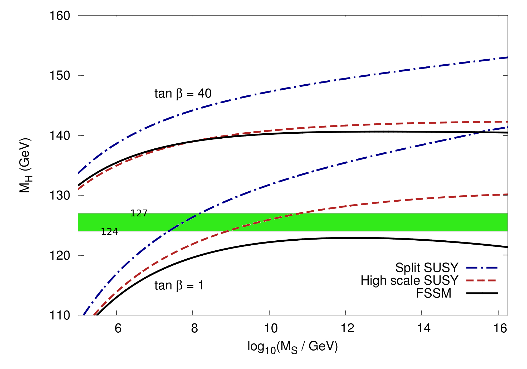
Figure 1: Higgs-mass predictions as a function of the SUSY scale $M_{\scriptscriptstyle S}$ for FSSM, High-Scale SUSY and Split SUSY. We set $M_{\tilde{g}^{\prime}}=\mu=2$ TeV and $\tan\beta=1$ or $40$. The green-shaded region indicates a Higgs mass in the range $[124,127]$ GeV.

We find that, in the FSSM, the dependence of the physical Higgs mass on the SUSY scale $M_{\scriptscriptstyle S}$ differs markedly from the cases of regular Split SUSY or High-Scale SUSY (where all superparticle masses are set to the scale $M_{\scriptscriptstyle S}$). Figure 1 illustrates this discrepancy, showing $M_{\scriptscriptstyle H}$ as a function of $M_{\scriptscriptstyle S}$ for $M_{\tilde{g}^{\prime}}=\mu=2$ TeV. The solid (black) curves represent the prediction of the FSSM, the dashed (red) ones represent the prediction of High-Scale SUSY, and the dot-dashed (blue) ones represent the prediction of regular Split SUSY (the predictions for the latter two models were obtained with appropriate modifications of the FSSM calculation described in section 4.1). For each model, the lower curves were obtained with $\tan\beta=1$, resulting in the lowest possible value of $M_{\scriptscriptstyle H}$ for a given $M_{\scriptscriptstyle S}$, while the upper curves were obtained with $\tan\beta=40$.

As was shown earlier in ref. [7], the Higgs mass grows monotonically with the SUSY scale $M_{\scriptscriptstyle S}$ in the Split-SUSY case, while it reaches a plateau in High-Scale SUSY. In both cases, the prediction for the Higgs mass falls between $124$ and $127$ GeV only for a relatively narrow range of $M_{\scriptscriptstyle S}$, well below the unification scale $M_{\rm{\scriptscriptstyle GUT}}\approx 2\!\times\!10^{16}$ GeV. In the FSSM, on the other hand, the Higgs mass reaches a maximum and then starts decreasing, remaining generally lower than in the other models. It is therefore much easier to obtain a Higgs mass close to the experimentally observed value even for large values of the SUSY scale. For example, as will be discussed later, when $\tan\beta\approx 1.5$ we find that the FSSM prediction for the Higgs mass falls between $124$ and $127$ GeV for all values of $M_{\scriptscriptstyle S}$ between $10^{8}$ GeV and $M_{\rm{\scriptscriptstyle GUT}}\,$.

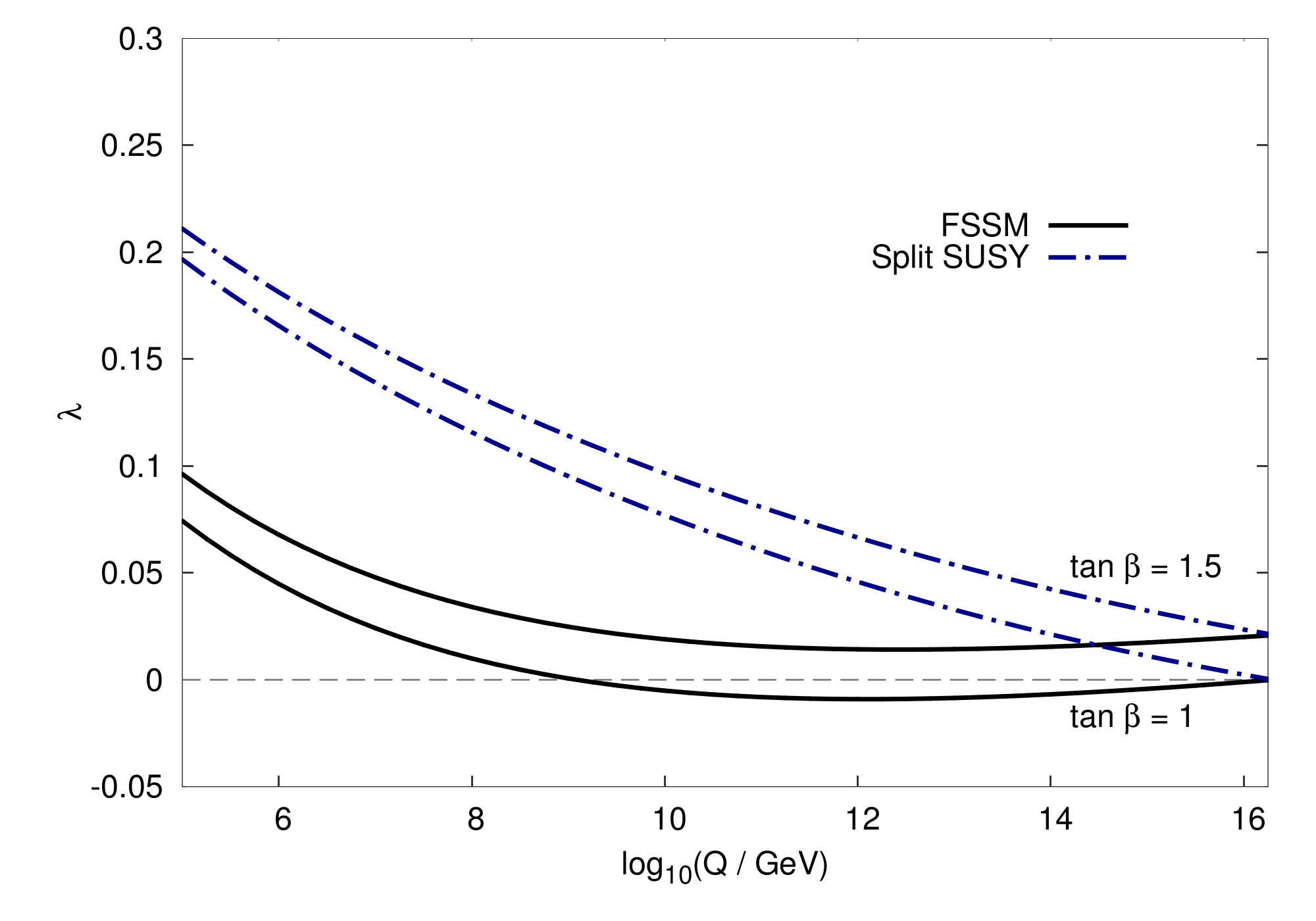
Figure 2: Running of the Higgs quartic coupling $\lambda$ in the FSSM and in the usual Split-SUSY case for $\tan\beta=1$ and $1.5$. We set $M_{\scriptscriptstyle S}=2\!\times\!10^{16}$ GeV and $M_{\tilde{g}^{\prime}}=\mu=2$ TeV.

This new behaviour originates in the RG evolution of $\lambda$ in the FSSM, which differs from the case of Split SUSY. In figure 2 we show the dependence of $\lambda$ on the renormalisation scale $Q$ in the two theories, imposing the boundary condition in eq. (4.1) at the scale $M_{\scriptscriptstyle S}=2\!\times\!10^{16}$ and setting $\tan\beta$ to either $1$ or $1.5$. Even though we impose the same boundary condition in both theories, the fact that the effective Higgs–higgsino–gaugino couplings are zero in the FSSM induces a different evolution. Indeed, in Split SUSY the contributions proportional to four powers of the Higgs–higgsino–gaugino couplings enter the one-loop part of $\beta_{\lambda}$ with negative sign, as do those proportional to four powers of the top Yukawa coupling, whereas the contributions proportional to four powers of the gauge couplings enter with positive sign. For $M_{\scriptscriptstyle S}\gtrsim 10^{12}$ GeV, the top Yukawa coupling is sufficiently suppressed at the matching scale that removing the Higgs–higgsino–gaugino couplings makes $\beta_{\lambda}$ positive. This prompts $\lambda$ to decrease with decreasing $Q$, until the negative contribution of the top Yukawa coupling takes over and $\lambda$ begins to increase.

Figure 2 also shows that, for values of $\tan\beta$ sufficiently close to 1, the quartic coupling $\lambda$ can become negative during its evolution down from the scale $M_{\scriptscriptstyle S}$, only to become positive again when $Q$ approaches the weak scale. This points to an unstable vacuum, and a situation similar to the one described in ref. [38]. However, it was already clear from figure 1 that, for $\tan\beta=1$, the FSSM prediction for the Higgs mass is too low anyway. For the values of $\tan\beta$ large enough to induce a Higgs mass in the observed range, the theory is stable. This is illustrated in figure 3, where we show the contours of equal Higgs mass on the $M_{\scriptscriptstyle S}\,$–$\,\tan\beta$ plane, setting $M_{\tilde{g}^{\prime}}=\mu=2$ TeV. The green-shaded region corresponds to a Higgs mass in the observed range between $124$ and $127$ GeV, while the yellow-shaded region is where $\lambda$ becomes negative during its evolution between $M_{\scriptscriptstyle S}$ and the weak scale, and the vacuum is unstable. It can be seen that, for $M_{\scriptscriptstyle S}\gtrsim 10^{8}$ GeV, a Higgs mass around $126$ GeV can be comfortably obtained for either $\tan\beta\approx 1.5$ or $\tan\beta\approx 0.6$. The unstable region is confined to values of $\tan\beta$ very close to $1$, and only for $M_{\scriptscriptstyle S}\gtrsim 10^{12}$ GeV. For lower values of $M_{\scriptscriptstyle S}$, the top Yukawa coupling is not sufficiently suppressed at the matching scale and $\beta_{\lambda}$ is always negative, therefore there is no region of instability.

We investigated how our results are affected by the experimental uncertainty on the top mass. An increase (or decrease) of $1$ GeV from the central value $M_{t}=173.2$ GeV used in figure 3 translates into an increase (or decrease) in our prediction for the Higgs mass of $1$–$2$ GeV, depending on $M_{\scriptscriptstyle S}$. For larger values of $M_{t}$, the observed value of $M_{\scriptscriptstyle H}$ is obtained for $\tan\beta$ closer to $1$, and the green regions in figure 3 approach the unstable region. The size of the unstable region is itself dependent on $M_{t}$ (i.e. the region shrinks for larger $M_{t}$) but the effect is much less pronounced. Consequently, raising the value of the top mass may lead to instability for large $M_{\scriptscriptstyle S}$ (e.g. for $M_{\scriptscriptstyle S}\gtrsim 10^{12}$ GeV when $M_{\tilde{g}^{\prime}}=2$ TeV). Considering an extreme case, for $M_{t}=175$ GeV we would see a substantial overlap of the experimentally acceptable regions with the unstable region around $M_{\scriptscriptstyle S}\approx M_{\rm{\scriptscriptstyle GUT}}$. On the other hand, for values of $M_{t}$ lower than $173.2$ GeV the green regions in figure 3 are shifted towards values of $\tan\beta$ further away from $1$, and the vacuum is always stable for the correct Higgs mass.

Finally, in figure 4 we show the contours of equal Higgs mass on the $M_{\tilde{g}^{\prime}}\,$–$\,\tan\beta$ plane, setting $M_{\scriptscriptstyle S}=2\!\times\!10^{16}$ GeV and $\mu=2$ TeV. The colour code is the same as in figure 3. It can be seen that the region where the FSSM prediction for the Higgs mass is between $124$ and $127$ GeV gets closer to the unstable region when the F-gluino mass increases. However, the dependence of $M_{\scriptscriptstyle H}$ on $M_{\tilde{g}^{\prime}}$ is relatively mild, and only when $M_{\tilde{g}^{\prime}}$ is in the multi-TeV region do the green and yellow regions in figure 4 overlap. We conclude that if we insist on enforcing exact stability and setting $M_{\scriptscriptstyle S}\approx 2\!\times\!10^{16}$ GeV, then obtaining a Higgs mass compatible with the observed value constrains the gluino mass to the few-TeV region.

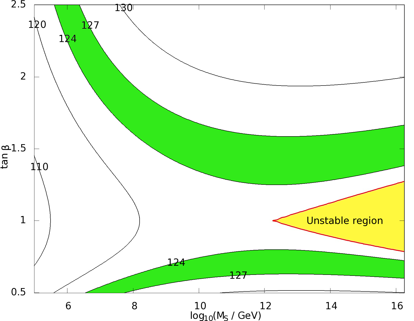
Figure 3: Contour plot of the prediction for the Higgs mass on the $M_{\scriptscriptstyle S}\,$–$\,\tan\beta$ plane, for $M_{\tilde{g}^{\prime}}=\mu=2$ TeV. The yellow-shaded region indicates where $\lambda$ becomes negative during its running between $M_{\scriptscriptstyle Z}$ and $M_{\scriptscriptstyle S}$. The green-shaded region indicates a Higgs mass in the range $[124,127]$ GeV.

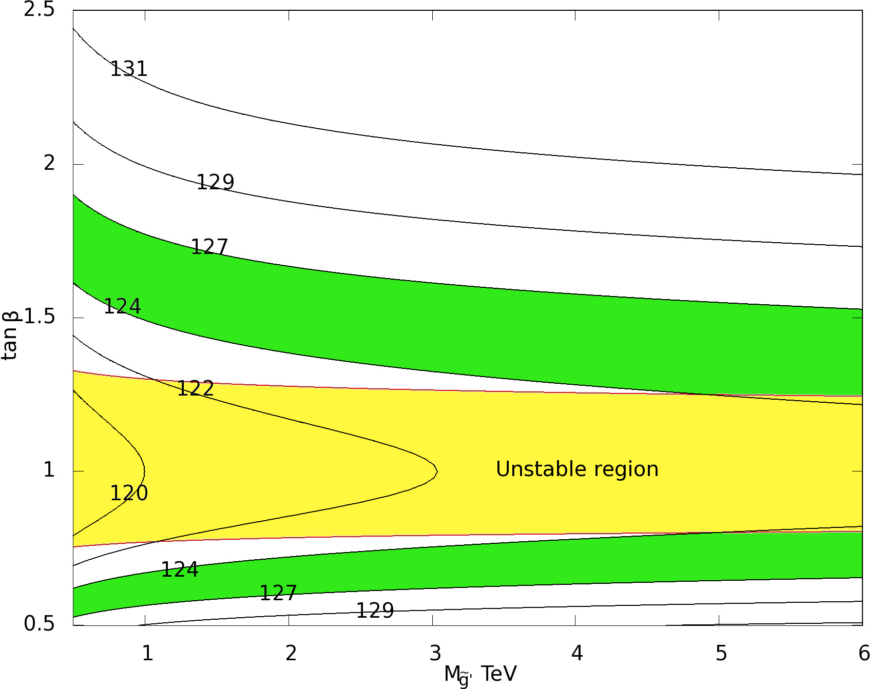
Figure 4: Same as figure 3 on the $M_{\tilde{g}^{\prime}}\,$–$\,\tan\beta$ plane, with $M_{\scriptscriptstyle S}=2\!\times\!10^{16}$ GeV and $\mu=2$ TeV.

5 Conclusions

We have defined a model – the FSSM – which has the same particle content at low energies as Split SUSY, but has a substantially different ultraviolet completion and also low-energy phenomenology:

1. We discussed in section 2.2 that the F-gaugino and F-higgsino couplings to the Higgs are suppressed by $\varepsilon^{2}$.

2. The effective operators leading to the decay of the charginos/heavier neutralinos, which are generated by integrating out the sfermions, are also suppressed, because the adjoint fermions $\chi$ do not have a gauge-current coupling to the sfermions. As discussed in section 3, the lifetimes are enhanced by a factor $\varepsilon^{-4}$. This makes the gauginos/higgsinos very long-lived; we must appeal to a non-thermal history of the universe with a low reheating temperature to avoid unwanted relics.

3. Since we no longer have an $R$-symmetry, the usual corrections to the Higgs quartic coupling at the SUSY scale proportional to powers of $|A_{t}-\mu_{0}\cot\beta|^{2}/M_{\scriptscriptstyle S}^{2}$ are in principle no longer negligible. However, as we discussed in section 4, in Split-SUSY scenarios those corrections are less important than in the MSSM, because the evolution to the large scale $M_{\scriptscriptstyle S}$ suppresses the top Yukawa coupling that multiplies them [6, 7].

4. Finally, the main result of this paper was presented in section 4, and concerns the precision determination of the Higgs mass in this model. Its value is substantially different than in either High-Scale or Split SUSY; in particular we can find $126$ GeV for any SUSY scale, with a vacuum that is always stable when the F-gluino mass is not too large.

We have found that a standard-model-like Higgs boson with a mass around $126$ GeV can be obtained for low values of $\tan\beta$. For low values of $M_{\scriptscriptstyle S}$, the exact value of $\tan\beta$ is subject to modification that we estimated when considering the presence of additional contributions to the quartic Higgs coupling from the unsuppressed $A$-terms. For larger values of $M_{\scriptscriptstyle S}$, the latter contributions are negligible.

In supersymmetric theories, the theorem of non-renormalisation of the superpotential implies that supersymmetry cannot be broken by perturbative effects. It is either broken at tree level or by non-perturbative effects. The former implies that the scale of supersymmetry breaking is of the order of the fundamental (string) scale $M_{*}$, and unless this is taken to lie at an intermediate energy scale [39], it predicts a heavy spectrum. In studies of low-energy supersymmetry, the use of non-perturbative effects attracted most interest because it allows the generation of the required large hierarchy of scales through dimensional transmutation. It is then interesting to investigate the fate of the former possibility when the supersymmetry scale is pushed to higher values. For Split and High-Scale SUSY, it is difficult to justify a very high $\mathcal{O}(M_{\rm{\scriptscriptstyle GUT}})$ SUSY scale, since in that regime they predict the Higgs mass to be too high (unless one pushes to the limits of the theoretical and experimental uncertainties, see e.g. refs[7, 40]).

Here, we have shown that the situation is different in the Fake Split SUSY Model. It is tempting to consider that while supersymmetry is broken at tree level in a secluded sector, the scale $M_{\scriptscriptstyle S}\sim M_{\rm{\scriptscriptstyle GUT}}$ could be induced through radiative effects [17] from the fundamental scale $M_{\scriptscriptstyle S}\sim\alpha M_{*}\,$, where $\alpha$ is a loop factor. We postpone the construction of explicit realisations of this possibility for a future study.

Appendix: Two-loop RGEs for Split-SUSY masses

In this appendix we list the two-loop RGEs for the fermion-mass parameters of Split SUSY in the ${\overline{\rm MS}}$ scheme. Defining

$$\frac{dm_{x}}{d\ln Q}=\frac{\beta^{(1)}_{m_{x}}}{16\pi^{2}}~{}+~{}\frac{\beta^{(2)}_{m_{x}}}{256\pi^{4}}\,,~{}~{}~{}~{}~{}~{}~{}~{}(m_{x}=m_{\tilde{g}},\,m_{\tilde{\scriptscriptstyle B}},\,m_{\tilde{\scriptscriptstyle W}},\,\mu)~{},$$ (A1)

we obtained, using the public codes SARAH [34] and PyR@TE [35],

$$\beta_{m_{\tilde{g}}}^{(1)} = -18g_{3}^{2}m_{\tilde{g}}~{},~{}~{}~{}~{}~{}~{}~{}~{}~{}~{}\beta_{m_{\tilde{g}}}^{(2)}~{}=~{}-228g_{3}^{4}m_{\tilde{g}}~{},$$ (A2)

$$\beta_{m_{\tilde{\scriptscriptstyle B}}}^{(1)} = (\tilde{g}_{1\mathrm{u}}^{2}+\tilde{g}_{1\mathrm{d}}^{2})m_{\tilde{\scriptscriptstyle B}}+4\tilde{g}_{1\mathrm{d}}\tilde{g}_{1\mathrm{u}}\mu~{},$$ (A3)

$$\beta_{m_{\tilde{\scriptscriptstyle B}}}^{(2)} = \left[\frac{1}{8}\left(\tilde{g}_{1\mathrm{u}}^{4}+\tilde{g}_{1\mathrm{d}}^{4}\right)-\frac{7}{2}\tilde{g}_{1\mathrm{d}}^{2}\tilde{g}_{1\mathrm{u}}^{2}-\frac{21}{8}\left(\tilde{g}_{1\mathrm{u}}^{2}\tilde{g}_{2\mathrm{u}}^{2}+\tilde{g}_{1\mathrm{d}}^{2}\tilde{g}_{2\mathrm{d}}^{2}\right)-\frac{9}{4}\left(\tilde{g}_{1\mathrm{u}}^{2}\tilde{g}_{2\mathrm{d}}^{2}+\tilde{g}_{1\mathrm{d}}^{2}\tilde{g}_{2\mathrm{u}}^{2}\right)\right.$$ (A4)

$$\left.\,\,\,\,+\frac{51}{8}\,\left(\tilde{g}_{1\mathrm{u}}^{2}+\tilde{g}_{1\mathrm{d}}^{2}\right)\left(\frac{1}{5}g_{1}^{2}+g_{2}^{2}\right)-\frac{3}{2}\left({\tilde{g}_{1\mathrm{u}}^{2}+\tilde{g}_{1\mathrm{d}}^{2}}\right)\left(3g_{b}^{2}+3g_{t}^{2}+g_{\tau}^{2}\right)\right]m_{\tilde{\scriptscriptstyle B}}$$

$$+ \left[3\tilde{g}_{2\mathrm{d}}^{2}\tilde{g}_{1\mathrm{d}}^{2}+3\tilde{g}_{2\mathrm{u}}^{2}\tilde{g}_{1\mathrm{u}}^{2}-6\tilde{g}_{2\mathrm{d}}\tilde{g}_{1\mathrm{d}}\tilde{g}_{2\mathrm{u}}\tilde{g}_{1\mathrm{u}}\right]m_{\tilde{\scriptscriptstyle W}}$$

$$+ \left[\frac{24}{5}g_{1}^{2}+24g_{2}^{2}-\tilde{g}_{1\mathrm{u}}^{2}-\tilde{g}_{1\mathrm{d}}^{2}-3\tilde{g}_{2\mathrm{u}}^{2}-3\tilde{g}_{2\mathrm{d}}^{2}\right]\,\tilde{g}_{1\mathrm{d}}\tilde{g}_{1\mathrm{u}}\mu~{},$$

$$\beta_{m_{\tilde{\scriptscriptstyle W}}}^{(1)} = \left(-12g_{2}^{2}+\tilde{g}_{2\mathrm{u}}^{2}+\tilde{g}_{2\mathrm{d}}^{2}\right)m_{\tilde{\scriptscriptstyle W}}+4\tilde{g}_{2\mathrm{d}}\tilde{g}_{2\mathrm{u}}\mu~{},$$ (A5)

$$\beta_{m_{\tilde{\scriptscriptstyle W}}}^{(2)} = \left[-\frac{29}{8}\left(\tilde{g}_{2\mathrm{u}}^{4}+\tilde{g}_{2\mathrm{d}}^{4}\right)-\frac{21}{2}\tilde{g}_{2\mathrm{d}}^{2}\tilde{g}_{2\mathrm{u}}^{2}-\frac{7}{8}\left(\tilde{g}_{2\mathrm{u}}^{2}\tilde{g}_{1\mathrm{u}}^{2}+\tilde{g}_{2\mathrm{d}}^{2}\tilde{g}_{1\mathrm{d}}^{2}\right)-\frac{3}{4}\left(\tilde{g}_{2\mathrm{u}}^{2}\tilde{g}_{1\mathrm{d}}^{2}+\tilde{g}_{2\mathrm{d}}^{2}\tilde{g}_{1\mathrm{u}}^{2}\right)\right.$$ (A6)

$$\left.\,\,\,\,-\frac{233}{3}g_{2}^{4}+\frac{1}{8}\left(\tilde{g}_{2\mathrm{u}}^{2}+\tilde{g}_{2\mathrm{d}}^{2}\right)\left(\frac{51}{5}g_{1}^{2}+{91}g_{2}^{2}\right)-\frac{3}{2}\left(\tilde{g}_{2\mathrm{u}}^{2}+\tilde{g}_{2\mathrm{d}}^{2}\right)\left(3g_{b}^{2}+3g_{t}^{2}+g_{\tau}^{2}\right)\right]m_{\tilde{\scriptscriptstyle W}}$$

$$+ \left[\tilde{g}_{2\mathrm{u}}^{2}\tilde{g}_{1\mathrm{u}}^{2}+\tilde{g}_{2\mathrm{d}}^{2}\tilde{g}_{1\mathrm{d}}^{2}-2\tilde{g}_{2\mathrm{u}}\tilde{g}_{1\mathrm{u}}\tilde{g}_{2\mathrm{d}}\tilde{g}_{1\mathrm{d}}\right]m_{\tilde{\scriptscriptstyle B}}$$

$$+ \left[\frac{24}{5}g_{1}^{2}+48g_{2}^{2}-\tilde{g}_{1\mathrm{u}}^{2}-\tilde{g}_{1\mathrm{d}}^{2}-3\tilde{g}_{2\mathrm{u}}^{2}-3\tilde{g}_{2\mathrm{d}}^{2}\right]\,\tilde{g}_{2\mathrm{d}}\tilde{g}_{2\mathrm{u}}\mu~{},$$

$$\beta_{\mu}^{(1)} = \left(-\frac{9}{2}g_{2}^{2}-\frac{9}{10}g_{1}^{2}+\frac{3}{4}\tilde{g}_{2\mathrm{u}}^{2}+\frac{3}{4}\tilde{g}_{2\mathrm{d}}^{2}+\frac{1}{4}\tilde{g}_{1\mathrm{u}}^{2}+\frac{1}{4}\tilde{g}_{1\mathrm{d}}^{2}\right)\mu+3\tilde{g}_{2\mathrm{u}}\tilde{g}_{2\mathrm{d}}m_{\tilde{\scriptscriptstyle W}}+\tilde{g}_{1\mathrm{u}}\tilde{g}_{1\mathrm{d}}m_{\tilde{\scriptscriptstyle B}}~{},$$

$$\beta_{\mu}^{(2)} = \left[-\frac{421}{16}g_{2}^{4}+\frac{1359}{400}g_{1}^{4}-\frac{27}{40}g_{1}^{2}g_{2}^{2}-\frac{15}{8}\tilde{g}_{2\mathrm{u}}^{4}-\frac{15}{8}\tilde{g}_{2\mathrm{d}}^{4}-\frac{1}{4}\tilde{g}_{1\mathrm{u}}^{4}-\frac{1}{4}\tilde{g}_{1\mathrm{d}}^{4}\right.$$

$$\,\,\,\,+\frac{33}{160}g_{1}^{2}\left(\tilde{g}_{1\mathrm{u}}^{2}+\tilde{g}_{1\mathrm{d}}^{2}+3\tilde{g}_{2\mathrm{u}}^{2}+3\tilde{g}_{2\mathrm{d}}^{2}\right)+\frac{33}{32}g_{2}^{2}\left(\tilde{g}_{1\mathrm{u}}^{2}+\tilde{g}_{1\mathrm{d}}^{2}+11\tilde{g}_{2\mathrm{d}}^{2}+11\tilde{g}_{2\mathrm{u}}^{2}\right)$$

$$\,\,\,\,-\frac{9}{8}\left(\tilde{g}_{2\mathrm{u}}^{2}\tilde{g}_{1\mathrm{u}}^{2}+\tilde{g}_{2\mathrm{u}}^{2}\tilde{g}_{1\mathrm{d}}^{2}+\tilde{g}_{2\mathrm{d}}^{2}\tilde{g}_{1\mathrm{u}}^{2}+\tilde{g}_{2\mathrm{d}}^{2}\tilde{g}_{1\mathrm{d}}^{2}\right)-\frac{45}{4}\tilde{g}_{2\mathrm{d}}^{2}\tilde{g}_{2\mathrm{u}}^{2}-2\tilde{g}_{1\mathrm{d}}^{2}\tilde{g}_{1\mathrm{u}}^{2}$$

$$\left.\,\,\,\,+3\tilde{g}_{2\mathrm{d}}\tilde{g}_{1\mathrm{d}}\tilde{g}_{2\mathrm{u}}\tilde{g}_{1\mathrm{u}}-\frac{3}{8}\left(\tilde{g}_{1\mathrm{u}}^{2}+\tilde{g}_{1\mathrm{d}}^{2}+3\tilde{g}_{2\mathrm{u}}^{2}+3\tilde{g}_{2\mathrm{d}}^{2}\right)\left(3g_{t}^{2}+3g_{b}^{2}+g_{\tau}^{2}\right)\right]\mu$$

$$+ \left[\frac{87}{2}g_{2}^{2}+\frac{27}{10}g_{1}^{2}-3\tilde{g}_{2\mathrm{u}}^{2}-3\tilde{g}_{2\mathrm{d}}^{2}\right]\tilde{g}_{2\mathrm{u}}\tilde{g}_{2\mathrm{d}}m_{\tilde{\scriptscriptstyle W}}+\left[\frac{9}{2}g_{2}^{2}+\frac{9}{10}g_{1}^{2}-\tilde{g}_{1\mathrm{u}}^{2}-\tilde{g}_{1\mathrm{d}}^{2}\right]\tilde{g}_{1\mathrm{u}}\tilde{g}_{1\mathrm{d}}m_{\tilde{\scriptscriptstyle B}}\,.$$

Note Added

After the appearance of our paper in preprint, the author of ref. [33] revised his calculation of the two-loop RGEs in Split SUSY. His results for the RGEs of the fermion-mass parameters are now in full agreement with ours.

References

- [1] G. Aad et al. [ATLAS Collaboration], “Observation of a new particle in the search for the Standard Model Higgs boson with the ATLAS detector at the LHC,” Phys. Lett. B 716, 1 (2012) [arXiv:1207.7214 [hep-ex]].
- [2] S. Chatrchyan et al. [CMS Collaboration], “Observation of a new boson at a mass of 125 GeV with the CMS experiment at the LHC,” Phys. Lett. B 716, 30 (2012) [arXiv:1207.7235 [hep-ex]].
- [3] N. Arkani-Hamed and S. Dimopoulos, “Supersymmetric unification without low energy supersymmetry and signatures for fine-tuning at the LHC,” JHEP 0506 (2005) 073 [hep-th/0405159].
- [4] G. F. Giudice and A. Romanino, “Split supersymmetry,” Nucl. Phys. B 699 (2004) 65 [Erratum-ibid. B 706 (2005) 65] [hep-ph/0406088].
- [5] N. Arkani-Hamed, S. Dimopoulos, G. F. Giudice and A. Romanino, “Aspects of split supersymmetry,” Nucl. Phys. B 709 (2005) 3 [hep-ph/0409232].
- [6] N. Bernal, A. Djouadi and P. Slavich, “The MSSM with heavy scalars,” JHEP 0707 (2007) 016 [arXiv:0705.1496 [hep-ph]].
- [7] G. F. Giudice and A. Strumia, “Probing High-Scale and Split Supersymmetry with Higgs Mass Measurements,” Nucl. Phys. B 858 (2012) 63 [arXiv:1108.6077 [hep-ph]].
- [8] P. Fayet, “Massive Gluinos,” Phys. Lett. B 78, 417 (1978).
- [9] I. Antoniadis, K. Benakli, A. Delgado, M. Quiros and M. Tuckmantel, “Splitting extended supersymmetry,” Phys. Lett. B 634, 302 (2006) [arXiv:hep-ph/0507192];
- [10] I. Antoniadis, K. Benakli, A. Delgado, M. Quiros and M. Tuckmantel, “Split extended supersymmetry from intersecting branes,” Nucl. Phys. B 744, 156 (2006) [arXiv:hep-th/0601003].
- [11] M. S. Carena, A. Megevand, M. Quiros and C. E. M. Wagner, “Electroweak baryogenesis and new TeV fermions,” Nucl. Phys. B 716 (2005) 319 [hep-ph/0410352].
- [12] J. Unwin, “R-symmetric High Scale Supersymmetry,” Phys. Rev. D 86 (2012) 095002 [arXiv:1210.4936 [hep-ph]].
- [13] G. Belanger, K. Benakli, M. Goodsell, C. Moura and A. Pukhov, “Dark Matter with Dirac and Majorana Gaugino Masses,” JCAP 0908 (2009) 027 [arXiv:0905.1043 [hep-ph]].
- [14] E. Dudas, M. Goodsell, L. Heurtier and P. Tziveloglou, “Flavour models with Dirac and fake gluinos,” arXiv:1312.2011 [hep-ph].
- [15] K. Benakli, M. D. Goodsell, F. Staub and W. Porod, “A constrained minimal Dirac gaugino supersymmetric standard model”, in preparation.
- [16] K. Benakli and M. D. Goodsell, “Dirac Gauginos in General Gauge Mediation,” Nucl. Phys. B 816 (2009) 185 [arXiv:0811.4409 [hep-ph]].
- [17] K. Benakli and M. D. Goodsell, “Dirac Gauginos, Gauge Mediation and Unification,” Nucl. Phys. B 840 (2010) 1 [arXiv:1003.4957 [hep-ph]].
- [18] C. Csaki, J. Goodman, R. Pavesi and Y. Shirman, “The Problem of Dirac Gauginos and its Solutions,” arXiv:1310.4504 [hep-ph].
- [19] P. Gambino, G. F. Giudice and P. Slavich, “Gluino decays in split supersymmetry,” Nucl. Phys. B 726 (2005) 35 [hep-ph/0506214].
- [20] V. Khachatryan et al. [CMS Collaboration], “Search for Heavy Stable Charged Particles in collisions at TeV,” JHEP 1103 (2011) 024 [arXiv:1101.1645 [hep-ex]].
- [21] G. Aad et al. [ATLAS Collaboration], “Search for stable hadronising squarks and gluinos with the ATLAS experiment at the LHC,” Phys. Lett. B 701 (2011) 1 [arXiv:1103.1984 [hep-ex]].
- [22] S. Chatrchyan et al. [CMS Collaboration], “Searches for long-lived charged particles in pp collisions at =7 and 8 TeV,” arXiv:1305.0491 [hep-ex].
- [23] G. Aad et al. [ATLAS Collaboration], “Search for long-lived stopped R-hadrons decaying out-of-time with pp collisions using the ATLAS detector,” Phys. Rev. D 88 (2013) 112003 [arXiv:1310.6584 [hep-ex]].
- [24] A. Arvanitaki, C. Davis, P. W. Graham, A. Pierce and J. G. Wacker, “Limits on split supersymmetry from gluino cosmology,” Phys. Rev. D 72 (2005) 075011 [hep-ph/0504210].
- [25] E. Dudas, M. Goodsell and P. Tziveloglou, “Goldstini and Dirac gaugino masses,” in preparation.
- [26] T. K. Hemmick, D. Elmore, T. Gentile, P. W. Kubik, S. L. Olsen, D. Ciampa, D. Nitz and H. Kagan et al., “A Search for Anomalously Heavy Isotopes of Low Nuclei,” Phys. Rev. D 41 (1990) 2074.
- [27] P. F. Smith, J. R. J. Bennett, G. J. Homer, J. D. Lewin, H. E. Walford and W. A. Smith, “A Search For Anomalous Hydrogen In Enriched D-2 O, Using A Time-of-flight Spectrometer,” Nucl. Phys. B 206 (1982) 333.
- [28] J. Beringer et al. [Particle Data Group Collaboration], “Review of Particle Physics (RPP),” Phys. Rev. D 86 (2012) 010001.
- [29] M. Muether [Tevatron Electroweak Working Group and CDF and D0 Collaborations], “Combination of CDF and DO results on the mass of the top quark using up to at the Tevatron,” arXiv:1305.3929 [hep-ex].
- [30] J. Fleischer, F. Jegerlehner, O. V. Tarasov and O. L. Veretin, “Two loop QCD corrections of the massive fermion propagator,” Nucl. Phys. B 539 (1999) 671 [Erratum-ibid. B 571 (2000) 511] [hep-ph/9803493].
- [31] L. V. Avdeev and M. Y. Kalmykov, “Pole masses of quarks in dimensional reduction,” Nucl. Phys. B 502 (1997) 419 [hep-ph/9701308].
- [32] M. Binger, “Higgs boson mass in split supersymmetry at two-loops,” Phys. Rev. D 73 (2006) 095001 [hep-ph/0408240].
- [33] C. Tamarit, “Decoupling heavy sparticles in hierarchical SUSY scenarios: Two-loop Renormalization Group equations,” arXiv:1204.2292 [hep-ph].
- [34] F. Staub, “SARAH 4: A tool for (not only SUSY) model builders,” arXiv:1309.7223 [hep-ph].
- [35] F. Lyonnet, I. Schienbein, F. Staub and A. Wingerter, “PyR@TE: Renormalization Group Equations for General Gauge Theories,” arXiv:1309.7030 [hep-ph].
- [36] A. Sirlin and R. Zucchini, “Dependence of the Quartic Coupling H(m) on M() and the Possible Onset of New Physics in the Higgs Sector of the Standard Model,” Nucl. Phys. B 266 (1986) 389.
- [37] G. Degrassi, S. Di Vita, J. Elias-Miro, J. R. Espinosa, G. F. Giudice, G. Isidori and A. Strumia, “Higgs mass and vacuum stability in the Standard Model at NNLO,” JHEP 1208 (2012) 098 [arXiv:1205.6497 [hep-ph]].
- [38] D. Buttazzo, G. Degrassi, P. P. Giardino, G. F. Giudice, F. Sala, A. Salvio, A. Strumia, “Investigating the near-criticality of the Higgs boson,” [arXiv:1307.3536 [hep-ph]].
- [39] K. Benakli, “Phenomenology of low quantum gravity scale models,” Phys. Rev. D 60 (1999) 104002 [hep-ph/9809582].
- [40] A. Delgado, M. Garcia and M. Quiros, “Electroweak and supersymmetry breaking from the Higgs discovery,” arXiv:1312.3235 [hep-ph].