Signatures of anisotropic sources in the trispectrum of the cosmic microwave background

Abstract

Soft limits of $N$-point correlation functions, in which one wavenumber is much smaller than the others, play a special role in constraining the physics of inflation. Anisotropic sources such as a vector field during inflation generate distinct angular dependence in all these correlators. In this paper we focus on the four-point correlator (the trispectrum $T$). We adopt a parametrization motivated by models in which the inflaton $\phi$ is coupled to a vector field through a $I^{2}\left(\phi\right)F^{2}$ interaction, namely $T_{\zeta}({\bf k}_{1},{\bf k}_{2},{\bf k}_{3},{\bf k}_{4})\equiv\sum_{n}d_{n}[P_{n}(\hat{\bf k}_{1}\cdot\hat{\bf k}_{3})+P_{n}(\hat{\bf k}_{1}\cdot\hat{\bf k}_{12})+P_{n}(\hat{\bf k}_{3}\cdot\hat{\bf k}_{12})]P_{\zeta}(k_{1})P_{\zeta}(k_{3})P_{\zeta}(k_{12})+(23~{}{\rm perm})$, where $P_{n}$ denotes the Legendre polynomials. This shape is enhanced when the wavenumbers of the diagonals of the quadrilateral are much smaller than the sides, ${\bf k}_{i}$. The coefficient of the isotropic part, $d_{0}$, is equal to $\tau_{\rm NL}/6$ discussed in the literature. A $I^{2}\left(\phi\right)F^{2}$ interaction generates $d_{2}=2d_{0}$ which is, in turn, related to the quadrupole modulation parameter of the power spectrum, $g_{*}$, as $d_{2}\approx 14|g_{*}|N^{2}$ with $N\approx 60$. We show that $d_{0}$ and $d_{2}$ can be equally well-constrained: the expected 68% CL error bars on these coefficients from a cosmic-variance-limited experiment measuring temperature anisotropy of the cosmic microwave background up to $\ell_{\rm max}=2000$ are $\delta d_{2}\approx 4\delta d_{0}=105$. Therefore, we can reach $|g_{*}|=10^{-3}$ by measuring the angle-dependent trispectrum. The current upper limit on $\tau_{\rm NL}$ from the Planck temperature maps yields $|g_{*}|<0.02$ (95% CL).

UMN-TH-3317/13

1 Introduction

Cosmic inflation [1, 2, 3, 4, 5] is thought to have occurred in nearly de Sitter spacetime. Recent convincing detection of a small deviation from the exact scale invariance of primordial curvature perturbations [6, 7] shows that time-translation invariance is slightly broken during inflation. This provides strong evidence for inflation, as the expansion rate during inflation must be time-dependent in order for inflation to end eventually, and the time dependence must be weak in order for inflation to occur. This then leads to a natural question: “Are other symmetries also broken?”

Invariance under spatial rotation remains unbroken in the usual inflation models based on scalar fields; however, it can be broken in the presence of vector fields (see ref. [8, 9, 10] for reviews). In such a case, the two-point correlation function in Fourier space (power spectrum) of primordial curvature perturbations defined by $\langle\zeta_{{\bf k}_{1}}\zeta_{{\bf k}_{2}}\rangle=(2\pi)^{3}\delta^{(3)}({\bf k}_{1}+{\bf k}_{2})P_{\zeta}({\bf k}_{1})$ generically exhibits a direction dependence as [11]

$$P_{\zeta}({\bf k})=P_{0}(k)\left[1+g_{*}(k)(\hat{\bf k}\cdot\hat{\bf E}_{\rm cl})^{2}\right],$$ (1.1)

where $\hat{\bf E}_{\rm cl}$ is a preferred direction in space and $P_{0}(k)$ is the isotropic power spectrum. The amplitude, $g_{*}(k)$, may depend on wavenumbers.

Temperature anisotropy of the cosmic microwave background (CMB) offers a stringent test of rotational invariance of correlation functions. Assuming that $g_{*}$ is independent of wavenumbers (which is a reasonable assumption for inflation models we mostly focus on in this paper, up to a logarithmic correction), ref. [12] finds $g_{*}=0.002\pm 0.016$ (68% CL) from the temperature data obtained recently by the Planck satellite [13]. The 95% CL limit is $-0.030<g_{*}<0.034$. This measurement was achieved after removing statistical anisotropy caused by elliptical beams of the Planck satellite [14] and emission from our own Galaxy [15].

The three-point function (bispectrum) offers an additional test of rotational invariance of correlation functions. As breaking of rotational invariance during inflation requires multiple fields (e.g., a scalar field driving inflation and a vector field), it also breaks the so-called single-field consistency relation of the bispectrum [16, 17]; namely, there can be a non-negligible correlation in a “soft limit” of the three-point correlation function, in which one wavenumber, say $k_{3}$, is much smaller than the other two, i.e., $k_{3}\ll k_{1}\approx k_{2}$. Breaking of rotational invariance then introduces a dependence of the soft-limit bispectrum on angles between the wavenumbers. Defining the bispectrum as $\langle\zeta_{{\bf k}_{1}}\zeta_{{\bf k}_{2}}\zeta_{{\bf k}_{3}}\rangle=(2\pi)^{3}\delta^{(3)}({\bf k}_{1}+{\bf k}_{2}+{\bf k}_{3})B_{\zeta}(k_{1},k_{2},k_{3})$, we write [18]

$$B_{\zeta}(k_{1},k_{2},k_{3})=\sum_{n}c_{n}P_{n}(\hat{\bf k}_{1}\cdot\hat{\bf k}_{2})P_{\zeta}(k_{1})P_{\zeta}(k_{2})+(\mbox{2 perm}),$$ (1.2)

where $P_{n}(x)$ denotes the Legendre polynomials. Note that this form is valid for an isotropic measurement of the bispectrum, namely for the case in which we fix a triangular shape, and we then average over all possible orientations of this shape in Fourier space (this is equivalent to taking an average over all possible directions for the preferred direction $\hat{\bf E}_{\rm cl}$). The Planck temperature data give constraints on the first three coefficients as $c_{0}=3.2\pm 7.0$, $c_{1}=11.0\pm 113$, and $c_{2}=3.8\pm 27.8$ ($68\%$ CL) [19]. Given a model of inflation, these coefficients can be related to the parameter in the power spectrum, $g_{*}$. For example, the relation is $c_{0}=2c_{2}=320|g_{*}|(N/60)$ (with $N\approx 60$ being the number of $e$-folds counted from the end of inflation) for inflation models with a scalar field driving inflation, $\phi$, coupled to a vector field in the form of $I^{2}(\phi)F^{2}$ where $F$ is a vector-field strength tensor [20, 21, 18, 22, 23]. We then obtain $|g_{*}|<0.05$ and $0.36$ (95% CL) from $c_{0}$ and $c_{2}$, respectively.

The goal of this paper is to investigate the four-point function (trispectrum) defined by $\Braket{\prod_{i=1}^{4}\zeta_{{\bf k}_{i}}}_{c}=(2\pi)^{3}T_{\zeta}({\bf k}_{1},{\bf k}_{2},{\bf k}_{3},{\bf k}_{4})\delta^{(3)}\left(\sum_{i=1}^{4}{\bf k}_{i}\right)$, where $\langle\dots\rangle_{c}$ denotes the connected part of the trispectrum. The trispectrum is fully parametrized by six independent numbers, i.e., three wavenumbers and three angles between wavevectors, e.g., $k_{1}$, $k_{3}$, $k_{12}$, $\hat{\bf k}_{1}\cdot\hat{\bf k}_{3}$, $\hat{\bf k}_{1}\cdot\hat{\bf k}_{12}$, and $\hat{\bf k}_{3}\cdot\hat{\bf k}_{12}$, where ${\bf k}_{12}\equiv{\bf k}_{1}+{\bf k}_{2}$. We then find a simple linear parametrization as

$$T_{\zeta}({\bf k}_{1},{\bf k}_{2},{\bf k}_{3},{\bf k}_{4}) = \sum_{n}\left[A_{n}P_{n}(\hat{\bf k}_{1}\cdot\hat{\bf k}_{3})+B_{n}P_{n}(\hat{\bf k}_{1}\cdot\hat{\bf k}_{12})+C_{n}P_{n}(\hat{\bf k}_{3}\cdot\hat{\bf k}_{12})\right]$$ (1.3)

$$\times P_{\zeta}(k_{1})P_{\zeta}(k_{3})P_{\zeta}(k_{12})+(23~{}{\rm perm})~{}.$$

Symmetry under permutations of ${\bf k}_{i}$ imposes $B_{n}=C_{n}$, while $A_{n}$ remains independent in general. By construction, this trispectrum has the largest values in soft limits in which diagonals of a quadrilateral, $k_{12}$, etc., are much smaller than the sides, $k_{i}$.

Instead of studying the most general form, we shall study a simpler form motivated by inflation with $I^{2}(\phi)F^{2}$ coupling, which yields $A_{n}=B_{n}=C_{n}$ [18, 22, 23]. Our parametrization is

$$T_{\zeta}({\bf k}_{1},{\bf k}_{2},{\bf k}_{3},{\bf k}_{4}) = \sum_{n}d_{n}\left[P_{n}(\hat{\bf k}_{1}\cdot\hat{\bf k}_{3})+P_{n}(\hat{\bf k}_{1}\cdot\hat{\bf k}_{12})+P_{n}(\hat{\bf k}_{3}\cdot\hat{\bf k}_{12})\right]$$ (1.4)

$$\times P_{\zeta}(k_{1})P_{\zeta}(k_{3})P_{\zeta}(k_{12})+(23~{}{\rm perm})~{}.$$

The readers who are familiar with the primordial trispectrum would find that the first coefficient, $d_{0}$, is equal to $\tau_{\rm NL}/6$ in the literature [25]. Again, this form is valid for the trispectrum averaged over all possible directions of quadrilaterals (or $\hat{\bf E}_{\rm cl}$). As we shall show later in section 4, $I^{2}(\phi)F^{2}$ inflation gives $d_{0}=d_{2}/2\approx 7|g_{*}|N^{2}$. While $d_{2}$ is yet to be constrained by the data, the current upper limit on $d_{0}=\tau_{\rm NL}/6<470$ (95% CL) from the Planck data [19] yields $|g_{*}|<0.02$ (95% CL), which is already better than the limit from the power spectrum or the bispectrum. The limits on $d_{0}$ and $d_{2}$ from the next Planck data release should improve the limit further.

This paper is organized as follows. In section 2, we calculate the trispectrum of CMB temperature anisotropy from eq. (1.4) both with the flat-sky approximation and the full-sky formalism. In section 3, we calculate the expected 68% CL error bars on $d_{0}$ and $d_{2}$ from a cosmic-variance-limited CMB experiment. In section 4, we translate the error bars on $d_{0}$ and $d_{2}$ to that on $g_{*}$. We conclude in section 5.

2 Trispectrum of CMB temperature anisotropy

Let us rewrite the trispectrum given in eq. (1.4) as

$$\Braket{\prod_{i=1}^{4}\zeta_{{\bf k}_{i}}}_{c} = (2\pi)^{3}\int d^{3}{\bf K}\delta^{(3)}\left({\bf k}_{1}+{\bf k}_{2}+{\bf K}\right)\delta^{(3)}\left({\bf k}_{3}+{\bf k}_{4}-{\bf K}\right)\sum_{n}d_{n}{t}^{{\bf k}_{1}{\bf k}_{2}}_{{\bf k}_{3}{\bf k}_{4}}({\bf K},n)$$ (2.1)

$$+(23~{}{\rm perm})~{},$$

with

$${t}_{{\bf k}_{3}{\bf k}_{4}}^{{\bf k}_{1}{\bf k}_{2}}({\bf K},n) \equiv \left[P_{n}(\hat{\bf k}_{1}\cdot\hat{\bf k}_{3})+\frac{1+(-1)^{n}}{2}P_{n}(\hat{\bf k}_{1}\cdot\hat{\bf K})+\frac{1+(-1)^{n}}{2}P_{n}(\hat{\bf k}_{3}\cdot\hat{\bf K})\right]$$ (2.2)

$$\times P_{\zeta}(k_{1})P_{\zeta}(k_{3})P_{\zeta}(K)~{}.$$

Here, a reduced curvature trispectrum, ${t}_{{\bf k}_{3}{\bf k}_{4}}^{{\bf k}_{1}{\bf k}_{2}}({\bf K},n)$, satisfies ${t}_{{\bf k}_{3}{\bf k}_{4}}^{{\bf k}_{1}{\bf k}_{2}}({\bf K},n)={t}^{{\bf k}_{3}{\bf k}_{4}}_{{\bf k}_{1}{\bf k}_{2}}({\bf K},n)$. We then write eq. (2.2) using spherical harmonics as

$${t}_{{\bf k}_{3}{\bf k}_{4}}^{{\bf k}_{1}{\bf k}_{2}}({\bf K},n) = P_{\zeta}(k_{1})P_{\zeta}(k_{3})P_{\zeta}(K)\frac{4\pi}{2n+1}\sum_{\mu}$$ (2.3)

$$\times\left[Y_{n\mu}^{*}(\hat{\bf k}_{1})Y_{n\mu}(\hat{\bf k}_{3})+\frac{1+(-1)^{n}}{2}\left(Y_{n\mu}^{*}(\hat{\bf k}_{1})+Y_{n\mu}^{*}(\hat{\bf k}_{3})\right)Y_{n\mu}(\hat{\bf K})\right]~{}.$$

2.1 Flat-sky formula

To gain analytical insights into the structure of the CMB trispectrum, we first derive the CMB trispectrum in the flat-sky approximation. The coefficients of the two-dimensional Fourier transform of temperature anisotropy in a small flat section of the sky are related to the curvature perturbation as [26]

$$a({\boldsymbol{\ell}}) = \int_{0}^{\tau_{0}}d\tau\int_{-\infty}^{\infty}\frac{dk_{z}}{2\pi}\zeta\left({\bf k}^{\parallel}=-\frac{\boldsymbol{\ell}}{D},k_{z}\right)S_{I}\left(k=\sqrt{k_{z}^{2}+(\ell/D)^{2}},\tau\right)\frac{1}{D^{2}}e^{-ik_{z}D}~{},$$ (2.4)

where $D\equiv\tau_{0}-\tau$ denotes the conformal distance between a given conformal time, $\tau$, and the present time, $\tau_{0}$; ${\bf k}=({\bf k}^{\parallel},k_{z})$ with ${\bf k}^{\parallel}=(k_{x},k_{y})$; and $S_{I}$ is the so-called source function. The flat-sky approximation is accurate for $\ell\gg 1$.

The trispectrum of $a({\boldsymbol{\ell}})$ in the limits of $\ell_{i}\gg k_{i}D$ and $L\gg k_{z}r$ is given by

$$\Braket{\prod_{i=1}^{4}a({\boldsymbol{\ell}}_{i})}_{c} = (2\pi)^{2}\int d^{2}{\bf L}\delta^{(2)}\left(\boldsymbol{\ell}_{1}+\boldsymbol{\ell}_{2}+{\bf L}\right)\delta^{(2)}\left(\boldsymbol{\ell}_{3}+\boldsymbol{\ell}_{4}-{\bf L}\right)\sum_{n}d_{n}t^{\boldsymbol{\ell}_{1}\boldsymbol{\ell}_{2}}_{\boldsymbol{\ell}_{3}\boldsymbol{\ell}_{4}}({\bf L},n)$$ (2.5)

$$+(23~{}{\rm perm})~{},$$

where $t^{\boldsymbol{\ell}_{1}\boldsymbol{\ell}_{2}}_{\boldsymbol{\ell}_{3}\boldsymbol{\ell}_{4}}({\bf L},n)$ is the so-called CMB reduced trispectrum:

$$t^{\boldsymbol{\ell}_{1}\boldsymbol{\ell}_{2}}_{\boldsymbol{\ell}_{3}\boldsymbol{\ell}_{4}}({\bf L},n) \equiv \int_{-\infty}^{\infty}r^{2}dr\left[\prod_{i=1}^{4}\int_{0}^{\tau_{0}}d\tau_{i}\int_{\ell_{i}/D_{i}}^{\infty}\frac{dk_{i}}{2\pi}{\cal G}(\ell_{i},k_{i},\tau_{i},r)\right]P_{\zeta}(k_{1})P_{\zeta}(k_{3})P_{\zeta}\left(\frac{L}{|r|}\right)$$ (2.6)

$$\times\left[P_{n}(\hat{\boldsymbol{\ell}}_{1}\cdot\hat{\boldsymbol{\ell}}_{3})+\frac{1+(-1)^{n}}{2}P_{n}(\hat{\boldsymbol{\ell}}_{1}\cdot\hat{\bf L})+\frac{1+(-1)^{n}}{2}P_{n}(\hat{\boldsymbol{\ell}}_{3}\cdot\hat{\bf L})\right],$$

with

$${\cal G}(\ell,k,\tau,r)=\left[1-\left(\frac{\ell}{kD}\right)^{2}\right]^{-1/2}S_{I}\left(k,\tau\right)\frac{2}{D^{2}}\cos\left[\sqrt{1-\left(\frac{\ell}{kD}\right)^{2}}k(r-D)\right]~{}.$$ (2.7)

The flat-sky reduced CMB trispectrum directly reflects the angular dependence of the Legendre polynomials in the reduced curvature trispectrum, ${t}_{{\bf k}_{3}{\bf k}_{4}}^{{\bf k}_{1}{\bf k}_{2}}({\bf K},n)$, given in eq. (2.2).

Figure 1: Two shapes of the trispectrum in $\ell$ space in soft limits in which the diagonal, $L$, is much smaller than the sides, $\ell_{i}$. The red lines show $\ell_{1}$ and $\ell_{2}$, while the blue solid and dashed lines show two configurations of $\ell_{3}$ and $\ell_{4}$. Specifically, the blue solid and dashed lines show configurations in which $\hat{\boldsymbol{\ell}}_{1}\cdot\hat{\boldsymbol{\ell}}_{3}\approx-1$ and $1$, respectively. The black lines show the diagonal, $L$. (Top) Collinear configurations: $\hat{\boldsymbol{\ell}}_{1}\cdot\hat{\bf L}\approx-1$, $\hat{\boldsymbol{\ell}}_{3}\cdot\hat{\bf L}\approx\mp 1$, and $\hat{\boldsymbol{\ell}}_{1}\cdot\hat{\boldsymbol{\ell}}_{3}\approx\pm 1$. (Bottom) Isosceles configurations: $\hat{\boldsymbol{\ell}}_{1}\cdot\hat{\bf L}\approx\hat{\boldsymbol{\ell}}_{3}\cdot\hat{\bf L}\approx 0$, and $\hat{\boldsymbol{\ell}}_{1}\cdot\hat{\boldsymbol{\ell}}_{3}\approx\pm 1$.

The isotropic term, $n=0$, has the largest values when the diagonal, $L$, is much smaller than the sides, $\ell_{i}$, i.e., $\ell_{1}\approx\ell_{2}\gg L$ or $\ell_{3}\approx\ell_{4}\gg L$ [27]. The amplitude of the trispectrum in this limit is modulated when $n\neq 0$. For example, in the “collinear configurations,” $\hat{\boldsymbol{\ell}}_{1}\cdot\hat{\bf L}\approx-1$, $\hat{\boldsymbol{\ell}}_{3}\cdot\hat{\bf L}\approx\mp 1$, and $\hat{\boldsymbol{\ell}}_{1}\cdot\hat{\boldsymbol{\ell}}_{3}\approx\pm 1$ (see the top panel of figure 1), we find

$$t^{\boldsymbol{\ell}_{1}\boldsymbol{\ell}_{2}}_{\boldsymbol{\ell}_{3}\boldsymbol{\ell}_{4}}({\bf L},0):t^{\boldsymbol{\ell}_{1}\boldsymbol{\ell}_{2}}_{\boldsymbol{\ell}_{3}\boldsymbol{\ell}_{4}}({\bf L},1):t^{\boldsymbol{\ell}_{1}\boldsymbol{\ell}_{2}}_{\boldsymbol{\ell}_{3}\boldsymbol{\ell}_{4}}({\bf L},2)\approx 1:\pm\frac{1}{3}:1~{}.$$ (2.8)

In the “isosceles configurations,” $\hat{\boldsymbol{\ell}}_{1}\cdot\hat{\bf L}\approx\hat{\boldsymbol{\ell}}_{3}\cdot\hat{\bf L}\approx 0$, and $\hat{\boldsymbol{\ell}}_{1}\cdot\hat{\boldsymbol{\ell}}_{3}\approx\pm 1$ (see the bottom panel of figure 1), we find that the $n=2$ trispectrum vanishes:

$$t^{\boldsymbol{\ell}_{1}\boldsymbol{\ell}_{2}}_{\boldsymbol{\ell}_{3}\boldsymbol{\ell}_{4}}({\bf L},0):t^{\boldsymbol{\ell}_{1}\boldsymbol{\ell}_{2}}_{\boldsymbol{\ell}_{3}\boldsymbol{\ell}_{4}}({\bf L},1):t^{\boldsymbol{\ell}_{1}\boldsymbol{\ell}_{2}}_{\boldsymbol{\ell}_{3}\boldsymbol{\ell}_{4}}({\bf L},2)\approx 1:\pm\frac{1}{3}:0~{}.$$ (2.9)

Note that the sign of the $n=1$ trispectrum can change, as the Legendre polynomial with $n=1$ is an odd function. These signatures will affect the expected error bars on $d_{n}$ as discussed in section 3.

2.2 Full-sky formula

We shall move onto the full-sky formalism. The spherical harmonics coefficients of temperature anisotropy are related to the curvature perturbation as

$$a_{\ell m}=4\pi(-i)^{\ell}\int\frac{k^{2}dk}{(2\pi)^{3}}{\cal T}_{\ell}(k)\zeta_{\ell m}(k),$$ (2.10)

where $\zeta_{\ell m}(k)$ is the curvature perturbation in spherical harmonics space: $\zeta_{\ell m}(k)\equiv\int d^{2}\hat{\bf k}\zeta({\bf k})Y_{\ell m}^{*}(\hat{\bf k})$, and ${\cal T}_{\ell}(k)$ is the radiation transfer function, which is related to the source function as ${\cal T}_{\ell}(k)=\int_{0}^{\tau_{0}}d\tau~{}S_{I}(k,\tau)j_{\ell}(kD)$. Using this and the computational technique developed in ref. [28], the CMB trispectrum is given by

$$\Braket{\prod_{i=1}^{4}a_{\ell_{i}m_{i}}}_{c} = \left[\prod_{i=1}^{4}4\pi(-i)^{\ell_{i}}\int\frac{k_{i}^{2}dk_{i}}{(2\pi)^{3}}{\cal T}_{\ell_{i}}(k_{i})\right]\Braket{\prod_{i=1}^{4}\zeta_{\ell_{i}m_{i}}(k_{i})}_{c}~{},$$ (2.11)

where

$$\Braket{\prod_{i=1}^{4}\zeta_{\ell_{i}m_{i}}(k_{i})}_{c} = \sum_{LM}(-1)^{M}\left(\begin{array}[]{ccc}\ell_{1}&\ell_{2}&L\\ m_{1}&m_{2}&-M\end{array}\right)\left(\begin{array}[]{ccc}\ell_{3}&\ell_{4}&L\\ m_{3}&m_{4}&M\end{array}\right)$$ (2.17)

$$\times(2\pi)^{3}\sum_{n}d_{n}{t}_{k_{3}k_{4}\ell_{3}\ell_{4}}^{k_{1}k_{2}\ell_{1}\ell_{2}}(L,n)+(23~{}{\rm perm}),$$

and

$${t}_{k_{3}k_{4}\ell_{3}\ell_{4}}^{k_{1}k_{2}\ell_{1}\ell_{2}}(L,n) = P_{\zeta}(k_{1})P_{\zeta}(k_{3})\sum_{L_{1}L_{3}L^{\prime}}8^{2}(-1)^{\frac{L_{1}+\ell_{2}+L_{3}+\ell_{4}}{2}+\ell_{1}+\ell_{2}+\ell_{3}+\ell_{4}}$$ (2.18)

$$\times\int_{0}^{\infty}r^{2}dr\int_{0}^{\infty}r^{\prime 2}dr^{\prime}j_{L_{1}}(k_{1}r)j_{\ell_{2}}(k_{2}r)j_{L_{3}}(k_{3}r^{\prime})j_{\ell_{4}}(k_{4}r^{\prime})$$

$$\times\frac{\pi}{2}\left[F_{L^{\prime}L^{\prime}}(r,r^{\prime}){\cal I}_{\ell_{3}\ell_{4}}^{\ell_{1}\ell_{2}}(L_{1},L_{3},L^{\prime};n,L)+F_{L^{\prime}L}(r,r^{\prime}){\cal J}_{\ell_{3}\ell_{4}}^{\ell_{1}\ell_{2}}(L_{1},L_{3},L^{\prime};n,L)\right.$$

$$\left.\qquad+F_{LL^{\prime}}(r,r^{\prime}){\cal J}^{\ell_{3}\ell_{4}}_{\ell_{1}\ell_{2}}(L_{3},L_{1},L^{\prime};n,L)\right]~{}.$$

The $F$ function, defined by

$$F_{LL^{\prime}}(r,r^{\prime}) \equiv \frac{2}{\pi}\int K^{2}dKP_{\zeta}(K)j_{L}(Kr)j_{L^{\prime}}(Kr^{\prime})~{},$$ (2.19)

projects the $K$ dependence onto $L$. The ${\cal I}$ and ${\cal J}$ symbols are defined by

$${\cal I}_{\ell_{3}\ell_{4}}^{\ell_{1}\ell_{2}}(L_{1},L_{3},L^{\prime};n,L) \equiv \frac{4\pi}{2n+1}(-1)^{\ell_{2}+\ell_{4}+L^{\prime}+n+L}I_{L_{1}\ell_{2}L^{\prime}}I_{L_{3}\ell_{4}L^{\prime}}I_{\ell_{1}L_{1}n}I_{\ell_{3}L_{3}n}$$ (2.24)

$$\times(2L+1)\left\{\begin{array}[]{ccc}\ell_{1}&\ell_{2}&L\\ L^{\prime}&n&L_{1}\end{array}\right\}\left\{\begin{array}[]{ccc}\ell_{3}&\ell_{4}&L\\ L^{\prime}&n&L_{3}\end{array}\right\}~{},$$

$${\cal J}_{\ell_{3}\ell_{4}}^{\ell_{1}\ell_{2}}(L_{1},L_{3},L^{\prime};n,L) \equiv \frac{4\pi}{2n+1}\frac{1+(-1)^{n}}{2}(-1)^{\ell_{2}+L+\frac{L^{\prime}+L}{2}}I_{L^{\prime}Ln}I_{L_{1}\ell_{2}L^{\prime}}I_{\ell_{3}\ell_{4}L}I_{\ell_{1}L_{1}n}$$ (2.27)

$$\times\delta_{L_{3},\ell_{3}}\left\{\begin{array}[]{ccc}\ell_{1}&\ell_{2}&L\\ L^{\prime}&n&L_{1}\end{array}\right\}~{},$$

with $I_{l_{1}l_{2}l_{3}}\equiv\sqrt{\frac{(2l_{1}+1)(2l_{2}+1)(2l_{3}+1)}{4\pi}}\left(\begin{array}[]{ccc}l_{1}&l_{2}&l_{3}\\ 0&0&0\end{array}\right)$, and they reflect characteristic $\ell$ dependence imposed by $P_{n}(\hat{\bf k}_{1}\cdot\hat{\bf k}_{3})$ and $P_{n}(\hat{\bf k}_{1,3}\cdot\hat{\bf K})$, respectively. The selection rules in these symbols restrict summation ranges of $L_{1}$, $L_{3}$ and $L^{\prime}$ to the values close to $\ell_{1}$, $\ell_{3}$ and $L$, respectively. They also guarantee parity invariance of the trispectrum; namely, $\ell_{1}+\ell_{2}+\ell_{3}+\ell_{4}={\rm even}$ although $\ell_{1}+\ell_{2}$ or $\ell_{3}+\ell_{4}$ can take on both even and odd numbers in the ${\cal I}$ function. Substituting eq. (2.18) into eq. (2.11) leads to the final expression of the CMB trispectrum:

$$\Braket{\prod_{i=1}^{4}a_{\ell_{i}m_{i}}}_{c} = \sum_{LM}(-1)^{M}\left(\begin{array}[]{ccc}\ell_{1}&\ell_{2}&L\\ m_{1}&m_{2}&-M\end{array}\right)\left(\begin{array}[]{ccc}\ell_{3}&\ell_{4}&L\\ m_{3}&m_{4}&M\end{array}\right)$$ (2.33)

$$\times\sum_{n}d_{n}t_{\ell_{3}\ell_{4}}^{\ell_{1}\ell_{2}}(L,n)+(23~{}{\rm perm})~{},$$

where the reduced form is given by

$$t_{\ell_{3}\ell_{4}}^{\ell_{1}\ell_{2}}(L,n) \equiv \sum_{L_{1}L_{3}L^{\prime}}(-1)^{\frac{L_{1}+L_{3}+\ell_{1}+\ell_{3}}{2}+\ell_{1}+\ell_{3}}$$ (2.34)

$$\times\int_{0}^{\infty}r^{2}dr\int_{0}^{\infty}r^{\prime 2}dr^{\prime}\beta_{\ell_{1}L_{1}}(r)\alpha_{\ell_{2}}(r)\beta_{\ell_{3}L_{3}}(r^{\prime})\alpha_{\ell_{4}}(r^{\prime})$$

$$\times\left[F_{L^{\prime}L^{\prime}}(r,r^{\prime}){\cal I}_{\ell_{3}\ell_{4}}^{\ell_{1}\ell_{2}}(L_{1},L_{3},L^{\prime};n,L)+F_{L^{\prime}L}(r,r^{\prime}){\cal J}_{\ell_{3}\ell_{4}}^{\ell_{1}\ell_{2}}(L_{1},L_{3},L^{\prime};n,L)\right.$$

$$\left.\quad+F_{LL^{\prime}}(r,r^{\prime}){\cal J}^{\ell_{3}\ell_{4}}_{\ell_{1}\ell_{2}}(L_{3},L_{1},L^{\prime};n,L)\right]~{},$$

with

$$\alpha_{\ell}(r) = \frac{2}{\pi}\int k^{2}dk{\cal T}_{\ell}(k)j_{\ell}(kr)~{},$$ (2.35)

$$\beta_{\ell L}(r) = \frac{2}{\pi}\int k^{2}dkP_{\zeta}(k){\cal T}_{\ell}(k)j_{L}(kr)~{}.$$ (2.36)

When $n=0$, we have

$${\cal I}_{\ell_{3}\ell_{4}}^{\ell_{1}\ell_{2}}(L_{1},L_{3},L^{\prime};0,L) = {\cal J}_{\ell_{3}\ell_{4}}^{\ell_{1}\ell_{2}}(L_{1},L_{3},L^{\prime};0,L)={\cal J}^{\ell_{3}\ell_{4}}_{\ell_{1}\ell_{2}}(L_{3},L_{1},L^{\prime};0,L)$$ (2.37)

$$= I_{\ell_{1}\ell_{2}L}I_{\ell_{3}\ell_{4}L}\delta_{\ell_{1},L_{1}}\delta_{\ell_{3},L_{3}}\delta_{L^{\prime}L}~{},$$

which agrees with the previous results [29, 27].

The $r$ and $r^{\prime}$ integrals in eq. (2.34) are dominated by contributions from $r\simeq r^{\prime}\simeq r_{*}\equiv\tau_{0}-\tau_{*}$ with $\tau_{*}$ being the recombination epoch, as $\alpha_{\ell}(r)$ and $\beta_{\ell L}(r)$ peak at $r\simeq r_{*}$. If $F_{LL^{\prime}}(r,r^{\prime})$ varies slowly for $r\simeq r^{\prime}\simeq r_{*}$, i.e., in the small-$L$ limit, the $r$ and $r^{\prime}$ integrals may become separable:

$$t_{\ell_{3}\ell_{4}}^{\ell_{1}\ell_{2}}(L,n) \approx \sum_{L_{1}L_{3}L^{\prime}}(-1)^{\frac{L_{1}+L_{3}+\ell_{1}+\ell_{3}}{2}+\ell_{1}+\ell_{3}}R(\ell_{1},L_{1},\ell_{2})R(\ell_{3},L_{3},\ell_{4})$$ (2.38)

$$\times\left[F_{L^{\prime}L^{\prime}}(r_{*},r_{*}){\cal I}_{\ell_{3}\ell_{4}}^{\ell_{1}\ell_{2}}(L_{1},L_{3},L^{\prime};n,L)+F_{L^{\prime}L}(r_{*},r_{*}){\cal J}_{\ell_{3}\ell_{4}}^{\ell_{1}\ell_{2}}(L_{1},L_{3},L^{\prime};n,L)\right.$$

$$\left.\quad+F_{LL^{\prime}}(r_{*},r_{*}){\cal J}^{\ell_{3}\ell_{4}}_{\ell_{1}\ell_{2}}(L_{3},L_{1},L^{\prime};n,L)\right]~{},$$

where

$$R(\ell_{1},L_{1},\ell_{2})\equiv\int_{0}^{\infty}r^{2}dr\beta_{\ell_{1}L_{1}}(r)\alpha_{\ell_{2}}(r)~{}.$$ (2.39)

This approximate formula enables us to calculate the trispectrum in the whole $\ell$ space within a reasonable computational time. This approximation is justified, as the signal-to-noise of the trispectrum is dominated by soft limits in which $L$ is small [27]. Using a scale-invariant curvature power spectrum, $\frac{k^{3}P_{\zeta}(k)}{2\pi^{2}}=A_{S}$, we obtain $F_{LL^{\prime}}(r_{*},r_{*})$ as

$$F_{LL^{\prime}}(r_{*},r_{*})=\frac{\pi^{2}}{2}A_{S}\frac{\Gamma(\frac{L+L^{\prime}}{2})}{\Gamma(\frac{L-L^{\prime}+3}{2})\Gamma(\frac{L^{\prime}-L+3}{2})\Gamma(\frac{L+L^{\prime}+4}{2})}~{}.$$ (2.40)

Let us also derive eq. (2.38) from eq. (2.34) using the Sachs-Wolfe approximation. In the Sachs-Wolfe limit, the transfer function is given by ${\cal T}_{\ell}(k)\to-\frac{1}{5}j_{\ell}(kr_{*})$, and hence $\alpha_{\ell}(r)\to-\frac{1}{5r_{*}^{2}}\delta(r-r_{*})$. Performing the $r$ and $r^{\prime}$ integrals, we recover eq. (2.38) with $R(\ell_{1},L_{1},\ell_{2})\to\frac{1}{25}F_{\ell_{1}L_{1}}(r_{*},r_{*})$.

3 Expected error bars on $d_{0}$ and $d_{2}$

In this section, we calculate the expected 68% CL error bars on $d_{n}$ using the full-sky formalism. Let us define a Fisher matrix element for $d_{n}$ as [30]

$$F_{nn^{\prime}}\equiv\sum_{\ell_{1}>\ell_{2}>\ell_{3}>\ell_{4}}\sum_{L}\frac{T_{\ell_{3}\ell_{4}}^{\ell_{1}\ell_{2}}(L,n)T_{\ell_{3}\ell_{4}}^{\ell_{1}\ell_{2}}(L,n^{\prime})}{(2L+1)C_{\ell_{1}}C_{\ell_{2}}C_{\ell_{3}}C_{\ell_{4}}}~{},$$ (3.1)

where $C_{\ell}$ is the temperature power spectrum. We shall consider an ideal, noise-free, cosmic-variance limited experiment measuring temperature anisotropy up to a maximum multipole of $\ell_{\rm max}$; thus, $C_{\ell}$ contains the CMB only.

The trispectrum averaged over possible orientations of quadrilaterals, $T_{\ell_{3}\ell_{4}}^{\ell_{1}\ell_{2}}(L,n)$, is given by [30]

$$T_{\ell_{3}\ell_{4}}^{\ell_{1}\ell_{2}}(L,n) = P_{\ell_{3}\ell_{4}}^{\ell_{1}\ell_{2}}(L,n)+(2L+1)\sum_{L^{\prime}}\left[(-1)^{\ell_{2}+\ell_{3}}\left\{\begin{array}[]{ccc}\ell_{1}&\ell_{2}&L\\ \ell_{4}&\ell_{3}&L^{\prime}\end{array}\right\}P_{\ell_{2}\ell_{4}}^{\ell_{1}\ell_{3}}(L^{\prime},n)\right.$$ (3.7)

$$\left.\qquad\qquad\qquad\qquad\qquad+(-1)^{L+L^{\prime}}\left\{\begin{array}[]{ccc}\ell_{1}&\ell_{2}&L\\ \ell_{3}&\ell_{4}&L^{\prime}\end{array}\right\}P_{\ell_{3}\ell_{2}}^{\ell_{1}\ell_{4}}(L^{\prime},n)\right],~{}$$

with

$$P_{\ell_{3}\ell_{4}}^{\ell_{1}\ell_{2}}(L,n) = 2t_{\ell_{3}\ell_{4}}^{\ell_{1}\ell_{2}}(L,n)+2(-1)^{\ell_{1}+\ell_{2}+L}t_{\ell_{3}\ell_{4}}^{\ell_{2}\ell_{1}}(L,n)$$ (3.8)

$$+2(-1)^{\ell_{3}+\ell_{4}+L}t_{\ell_{4}\ell_{3}}^{\ell_{1}\ell_{2}}(L,n)+2(-1)^{\ell_{1}+\ell_{2}+\ell_{3}+\ell_{4}}t_{\ell_{4}\ell_{3}}^{\ell_{2}\ell_{1}}(L,n)~{}.$$

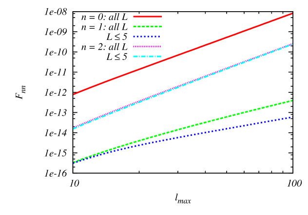
Figure 2: Diagonal elements of the Fisher matrix, $F_{00}$, $F_{11}$, and $F_{22}$, computed using the Sachs-Wolfe approximation. The lines with “all L” use all $L$ in the summation of the Fisher matrix, while the lines with “$L\leq 5$” for $n=1$ and 2 use only $L\leq 5$.

Figure 2 shows the diagonal elements of the Fisher matrix, $F_{00}$, $F_{11}$, and $F_{22}$, computed using the Sachs-Wolfe approximation. We show the results from summation over all possible diagonals, $L$, as well as those from summation over only soft limits, $L\leq 5$. We find that $F_{00}$ grows as $\ell_{\rm max}^{4}$ in agreement with the previous work [27], and $F_{22}$ also grows as $\ell_{\rm max}^{4}$; however, $F_{22}$ is smaller than $F_{00}$ by two orders magnitude. Most of information of the trispectrum with $n=2$ is contained in the soft limit, $L\leq 5$, just like that with $n=0$. On the other hand, $F_{11}$ grows more slowly as $\ell_{\rm max}^{3}$, implying that the error bar on $d_{1}$ would be too large to be useful. We thus do not consider $d_{1}$ any further in this paper. Information of the trispectrum with $n=1$ is not completely contained in the soft limit, and sizable contributions come from $L>5$.

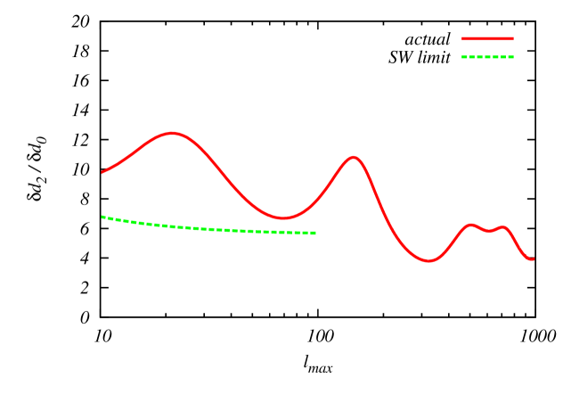
Figure 3: Ratio of the expected error bars, $\delta d_{2}/\delta d_{0}$. The solid line shows the results from eq. (2.38) with the full radiation transfer function, while the dashed line shows the Sachs-Wolfe approximation.

We now calculate the expected error bars on $d_{0}$ and $d_{2}$ when they are estimated jointly. We use

$${}^{(2)}F_{ij}=\left(\begin{array}[]{ccc}F_{00}&F_{02}\\ F_{02}&F_{22}\end{array}\right)~{},$$ (3.11)

to obtain

$$(\delta d_{0},\delta d_{2})=\left(\sqrt{{}^{(2)}F_{11}^{-1}},\sqrt{{}^{(2)}F_{22}^{-1}}\right).$$ (3.12)

In figure 3, we show the ratio of $\delta d_{2}$ to $\delta d_{0}$ as a function of $\ell_{\rm max}$. The error bar on $\delta d_{2}$ improves slightly faster than that on $\delta d_{0}$ as $\ell_{\rm max}$ increases. We find $\delta d_{2}/\delta d_{0}=4$ for $\ell_{\rm max}=1000$. We also find that these two parameters are not correlated very much: the cross-correlation coefficient, $F_{02}/\sqrt{F_{00}F_{22}}$, is as small as 0.2. For $\ell_{\rm max}=1000$, we find $(\delta d_{0},\delta d_{2})=(105,418)$. If a scaling relation $F_{00}\propto F_{22}\propto F_{02}\propto\ell_{\rm max}^{4}$ holds for $\ell_{\rm max}>1000$, the expected error bars on $d_{0}$ and $d_{2}$ would become $(\delta d_{0},\delta d_{2})=(26,105)$ for $\ell_{\rm max}=2000$. Recalling $d_{0}=\tau_{\rm NL}/6$, the error bar on $d_{0}$ we obtain here agrees with that given in ref. [27].

4 Expected error bar on $g_{*}$ from the CMB trispectrum

The parameters of the power spectrum ($g_{*}$), the bispectrum ($c_{n}$), and the trispectrum ($d_{n}$) can be related to each other once a model of inflation is specified. Such a relation is a powerful probe of the physics of inflation. In this section, we use inflation models with a particular coupling between a scalar field driving inflation and a vector field given by $I^{2}(\phi)F^{2}$ to relate the trispectrum parameters with $g_{*}$. The trispectrum averaged over all possible orientations of quadrilaterals is given by [18]

$$T_{\zeta}^{I^{2}F^{2}} \approx 24N^{2}|g_{*}|\left[(\hat{\bf k}_{1}\cdot\hat{\bf k}_{3})^{2}+(\hat{\bf k}_{1}\cdot\hat{\bf k}_{12})^{2}+(\hat{\bf k}_{3}\cdot\hat{\bf k}_{12})^{2}-(\hat{\bf k}_{1}\cdot\hat{\bf k}_{3})(\hat{\bf k}_{1}\cdot\hat{\bf k}_{12})(\hat{\bf k}_{3}\cdot\hat{\bf k}_{12})\right]$$ (4.1)

$$\times P_{\zeta}(k_{1})P_{\zeta}(k_{3})P_{\zeta}(k_{12})+(23{~{}\rm perm})~{},$$

where $N\approx 60$ is the number of $e$-folds counted from the end of inflation. The shape of this trispectrum is 99% correlated with the trispectrum without $(\hat{\bf k}_{1}\cdot\hat{\bf k}_{3})(\hat{\bf k}_{1}\cdot\hat{\bf k}_{12})(\hat{\bf k}_{3}\cdot\hat{\bf k}_{12})$. Adjusting the amplitude, we find that the following trispectrum is an excellent approximation to eq. (4.1):

$$T_{\zeta}^{I^{2}F^{2}} \approx 0.89\times 24N^{2}|g_{*}|\left[(\hat{\bf k}_{1}\cdot\hat{\bf k}_{3})^{2}+(\hat{\bf k}_{1}\cdot\hat{\bf k}_{12})^{2}+(\hat{\bf k}_{3}\cdot\hat{\bf k}_{12})^{2}\right]$$ (4.2)

$$\times P_{\zeta}(k_{1})P_{\zeta}(k_{3})P_{\zeta}(k_{12})+(23{~{}\rm perm})~{}.$$

The 99% correlation means that eqs. (4.1) and (4.2) have nearly identical shapes. The pre-factor 0.89 in eq. (4.2) is the ratio of the overall averages of trispectra computed numerically. One can understand this ratio by angular-averaging the trispectra in soft limits, using [23]: $(\hat{\bf k}_{1}\cdot\hat{\bf k}_{3})^{2}|_{\rm av}=1/3$, $(\hat{\bf k}_{1}\cdot\hat{\bf k}_{12})^{2}|_{\rm av}=(\hat{\bf k}_{3}\cdot\hat{\bf k}_{12})^{2}|_{\rm av}=1/2$, and $(\hat{\bf k}_{1}\cdot\hat{\bf k}_{3})(\hat{\bf k}_{1}\cdot\hat{\bf k}_{12})(\hat{\bf k}_{3}\cdot\hat{\bf k}_{12})|_{\rm av}=1/6$. This gives a very similar value of 0.875.

Comparing the above expression with eq. (1.4) yields the relationship between $d_{0}$, $d_{2}$ and $g_{*}$ as

$$d_{0}=\frac{1}{2}d_{2}\approx 0.89\times 2880\frac{|g_{*}|}{0.1}\left(\frac{N}{60}\right)^{2}~{}.$$ (4.3)

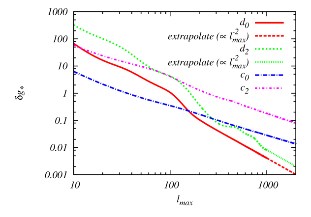
Figure 4: Expected 68% CL error bars on $g_{*}$ from the bispectrum parameters ($c_{0}$ and $c_{2}$ in eq. (1.4)) and the trispectrum parameters ($d_{0}$ and $d_{2}$), for $N=60$. The lines for the trispectrum in $\ell_{\rm max}>1000$ are extrapolation.

In figure 4, we show the expected error bars on $g_{*}$ computed from those on $d_{0}$ and $d_{2}$ using eq. (4.3). We show the results of the direct calculation of $\delta d_{0}$ and $\delta d_{2}$ up to $\ell_{\rm max}=1000$, and use the extrapolation for $1000<\ell_{\rm max}\leq 2000$. For comparison, we also show the error bars on $g_{*}$ from the bispectrum parameters using [18]

$$c_{0}=2c_{2}=32\frac{|g_{*}|}{0.1}\frac{N}{60}~{}.$$ (4.4)

Figure 5: Diagrams for the 2- (left), 3- (middle), and 4-point (right) functions of $\zeta\propto\delta\phi$ in the $I^{2}\left(\phi\right)F^{2}$ model. The external dashed lines are $\delta\phi$ lines, while the internal propagators are $\delta{\bf E}$ lines. The labels denote the momentum of the external lines, which is taken to flow inside the diagram. In the power spectrum, ${\bf k}_{1}+{\bf k}_{2}=0$, while in the other two diagrams we are interested in the soft-limit configurations ${\bf k}_{1}+{\bf k}_{2}\rightarrow 0$. A bullet denotes a mass insertion, namely a quadratic $\delta{\bf E}\;\delta\phi$ coupling proportional to the vector vacuum expectation value ${\bf E}_{\rm cl}$.

The trispectrum parameters are proportional to $|g_{*}|N^{2}$, whereas the bispectrum parameters are proportional to $|g_{*}|N$. More generally, we have

$$\langle\zeta^{n}\rangle\propto|g_{*}|N^{n-2}\;,$$ (4.5)

where $\zeta\propto-\frac{H}{\dot{\phi}}\,\delta\phi$ in uniform density gauge. To understand this scaling, consider the diagrams shown in figure 5, which represent the dominant contributions to $\langle\zeta^{2,3,4}\rangle$ arising from this interaction. By Taylor-expanding the $I^{2}\left(\phi\right)F^{2}$ coupling in the inflaton perturbations $\delta\phi\propto\zeta$, and by retaining only the linear terms,  we have the two interactions $H_{1}\propto\int d^{3}xa^{4}{\bf E}_{\rm cl}\cdot\delta{\bf E}\,\zeta$ and $H_{2}\propto\int d^{3}xa^{4}\delta{\bf E}\cdot\delta{\bf E}\,\zeta$. In this expression $H_{i}$ denotes a contribution to the interaction Hamiltonian, and $a$ is the scale factor ($a^{4}=\sqrt{-g}$ in conformal time $\tau$). For each value of $n$, the diagram shown in the figure corresponds to the following terms in the in-in formalism computation

$$\langle\zeta^{n}\left(\tau\right)\rangle\propto\left[\prod_{i=1}^{n-1}\int d\tau_{i}\right]\left\langle\left[\left[\dots\left[\zeta_{0}^{n}\left(\tau\right),H\left(\tau_{1}\right)\right],\dots\right],H\left(\tau_{n-1}\right)\right]\right\rangle\;,$$ (4.6)

where $\zeta_{0}$ denotes the (“unperturbed”) curvature perturbation in the absence of the $I^{2}\left(\phi\right)F^{2}$ term. We are interested in the correlators $\langle\zeta^{n}\rangle$ in the super-horizon regime. The integrals in eq. (4.6) are dominated by the regions in which also the fields arising from the vertices are in the super-horizon regime [21]. Each interaction contains one $\zeta_{0}\left(\tau_{i}\right)\propto\delta\phi\left(\tau_{i}\right)$ field which, once commuted with one of the external fields, gives $\left[\zeta_{0}\left(\tau\right),\zeta_{0}\left(\tau_{i}\right)\right]\propto\tau^{3}-\tau_{i}^{3}$ [21]. These commutators, and the measure $a^{4}\left(\tau_{i}\right)\propto\frac{1}{\tau_{i}^{4}}$ in each vertex, are the only time-dependent contributions to the integrand in eq. (4.6), leading to [21]

$$\langle\zeta^{n}\left(\tau\right)\rangle\propto\prod_{i}^{n-1}\int^{\tau}\frac{d\tau_{i}}{\tau_{i}}\left(\tau^{3}-\tau_{i}^{3}\right)\propto N^{n-1}~{}.$$ (4.7)

We thus see that the contribution to $\langle\zeta^{n}\rangle$ from the corresponding diagram in figure 5 is $\propto E_{\rm cl}^{2}\,N^{n-1}$. The diagram shown for the power spectrum ($n=2$ in this expression) adds up with the vacuum one, and provides the subdominant quadrupole modulation $\propto|g_{*}|\propto E_{\rm cl}^{2}\,N$. Therefore, $\langle\zeta^{n}\rangle\propto E_{\rm cl}^{2}\,N^{n-1}\propto|g_{*}|N^{n-2}$, as indicated in eq. (4.5). It is also worth noting that each internal line in the diagram produces in the final expression for $\langle\zeta^{n}\rangle$ a power spectrum which is function of the momentum carried on that line. For each given $n$, the diagram shown in the figure needs to be summed over with the diagrams obtained by permuting the position of the external lines. The diagrams shown in the figure factor out a $P_{\zeta}\left(k_{12}\right)$, and are enhanced in the soft limit $k_{12}\rightarrow 0$.

As a result of the scaling (4.5), if the error bars on $c_{n}$ and $d_{n}$ are equal, the trispectrum is more sensitive to $g_{*}$ than the bispectrum by a factor of $N\approx 60$. In addition, we find that the error bars on $g_{*}$ from the trispectrum decrease as $\delta g_{*}\propto\ell_{\rm max}^{-2}$, while those from the bispectrum decrease more slowly as $\delta g_{*}\propto\ell_{\rm max}^{-1}$. In reality, the error bars on the trispectrum parameters are much larger than those on the bispectrum parameters for smaller $\ell_{\rm max}$; thus, we find that the trispectrum yields smaller error bars on $g_{*}$ than the bispectrum for $\ell_{\rm max}\gtrsim 200$.

For $\ell_{\rm max}=2000$, we find $\delta g_{*}=1.0\times 10^{-3}$ and $2.0\times 10^{-3}$ from the $d_{0}$ and $d_{2}$ measurements, respectively. These error bars are an order of magnitude better than those expected from the bispectrum measurements, and are comparable to that expected from the power spectrum measurement for the same $\ell_{\rm max}$ (in the absence of systematic errors such as ellipticity of beams) [31].

5 Conclusion

Inflation models with anisotropic sources can create the perturbations with a preferred direction, and yield distinct angular dependence not only in the power spectrum and bispectrum, but also in the trispectrum of the CMB. Motivated by inflation models with $I^{2}(\phi)F^{2}$ coupling, we have studied the observational consequence of the parametrized form of the trispectrum given by eq. (1.4). The expected 68% CL error bars on the trispectrum parameters are $\delta d_{0}=26$ and $\delta d_{2}=105$ for a cosmic-variance-limited experiment measuring temperature anisotropy up to $\ell_{\rm max}=2000$. The error bar on $d_{1}$ is too large to be useful.

Using the prediction of inflation models with $I^{2}(\phi)F^{2}$ coupling, we derive the relationship between the trispectrum parameters and the power spectrum parameter, $g_{*}$. We then find that the trispectrum measurements can give competitive limit on $g_{*}$ reaching $\delta g_{*}=10^{-3}$ for $\ell_{\rm max}=2000$, which is an order of magnitude better than the expected limit from the bispectrum for the same $\ell_{\rm max}$. This is owing to two effects: the trispectrum parameters are proportional to $|g_{*}|N^{2}$ whereas the bispectrum parameters are proportional to $|g_{*}|N$; and the error bar on $g_{*}$ from the trispectrum decreases as $\ell_{\rm max}^{-2}$ whereas that from the bispectrum decreases as $\ell_{\rm max}^{-1}$.

The signatures of broken rotational invariance in the power spectrum [12] and the bispectrum [19] have been constrained by the temperature data of the Planck satellite. They have yielded the limit on $g_{*}$ of order $10^{-2}$. This limit can be improved further by using the trispectrum. The current limit on $d_{0}$ from the Planck data, $d_{0}=\tau_{\rm NL}/6<470$ (95% CL) [19], implies $|g_{*}|<0.02$ (95% CL), which is indeed competitive. The other parameter, $d_{2}$, has not been constrained by the data yet. Measurements of $d_{0}$ and $d_{2}$ from the full data of Planck should yield the best limit on $g_{*}$ within the context of inflation with $I^{2}(\phi)F^{2}$ coupling.

References

- [1] A. A. Starobinsky, A New Type of Isotropic Cosmological Models Without Singularity, Phys.Lett. B91 (1980) 99–102.
- [2] K. Sato, First Order Phase Transition of a Vacuum and Expansion of the Universe, Mon.Not.Roy.Astron.Soc. 195 (1981) 467–479.
- [3] A. H. Guth, The Inflationary Universe: A Possible Solution to the Horizon and Flatness Problems, Phys.Rev. D23 (1981) 347–356.
- [4] A. D. Linde, A New Inflationary Universe Scenario: A Possible Solution of the Horizon, Flatness, Homogeneity, Isotropy and Primordial Monopole Problems, Phys.Lett. B108 (1982) 389–393.
- [5] A. Albrecht and P. J. Steinhardt, Cosmology for Grand Unified Theories with Radiatively Induced Symmetry Breaking, Phys.Rev.Lett. 48 (1982) 1220–1223.
- [6] WMAP Collaboration, G. Hinshaw et. al., Nine-Year Wilkinson Microwave Anisotropy Probe (WMAP) Observations: Cosmological Parameter Results, Astrophys.J.Suppl. 208 (2013) 19, [arXiv:1212.5226].
- [7] Planck Collaboration Collaboration, P. Ade et. al., Planck 2013 results. XVI. Cosmological parameters, arXiv:1303.5076.
- [8] E. Dimastrogiovanni, N. Bartolo, S. Matarrese, and A. Riotto, Non-Gaussianity and statistical anisotropy from vector field populated inflationary models, Adv.Astron. 2010 (2010) 752670, [arXiv:1001.4049]. * Temporary entry *.
- [9] A. Maleknejad, M. Sheikh-Jabbari, and J. Soda, Gauge Fields and Inflation, Phys.Rept. 528 (2013) 161–261, [arXiv:1212.2921].
- [10] J. Soda, Statistical Anisotropy from Anisotropic Inflation, Class.Quant.Grav. 29 (2012) 083001, [arXiv:1201.6434].
- [11] L. Ackerman, S. M. Carroll, and M. B. Wise, Imprints of a Primordial Preferred Direction on the Microwave Background, Phys. Rev. D75 (2007) 083502, [astro-ph/0701357].
- [12] J. Kim and E. Komatsu, Limits on anisotropic inflation from the Planck data, Phys.Rev. D88 (2013) 101301, [arXiv:1310.1605].
- [13] Planck Collaboration Collaboration, P. Ade et. al., Planck 2013 results. I. Overview of products and scientific results, arXiv:1303.5062.
- [14] Planck Collaboration Collaboration, P. Ade et. al., Planck 2013 results. VII. HFI time response and beams, arXiv:1303.5068.
- [15] Planck Collaboration Collaboration, P. Ade et. al., Planck 2013 results. XII. Component separation, arXiv:1303.5072.
- [16] J. M. Maldacena, Non-Gaussian features of primordial fluctuations in single field inflationary models, JHEP 0305 (2003) 013, [astro-ph/0210603].
- [17] P. Creminelli and M. Zaldarriaga, Single field consistency relation for the 3-point function, JCAP 0410 (2004) 006, [astro-ph/0407059].
- [18] M. Shiraishi, E. Komatsu, M. Peloso, and N. Barnaby, Signatures of anisotropic sources in the squeezed-limit bispectrum of the cosmic microwave background, JCAP 1305 (2013) 002, [arXiv:1302.3056].
- [19] Planck Collaboration Collaboration, P. Ade et. al., Planck 2013 Results. XXIV. Constraints on primordial non-Gaussianity, arXiv:1303.5084.
- [20] N. Barnaby, R. Namba, and M. Peloso, Observable non-gaussianity from gauge field production in slow roll inflation, and a challenging connection with magnetogenesis, Phys.Rev. D85 (2012) 123523, [arXiv:1202.1469].
- [21] N. Bartolo, S. Matarrese, M. Peloso, and A. Ricciardone, The anisotropic power spectrum and bispectrum in the mechanism, Phys.Rev. D87 (2013) 023504, [arXiv:1210.3257].
- [22] A. A. Abolhasani, R. Emami, J. T. Firouzjaee, and H. Firouzjahi, formalism in anisotropic inflation and large anisotropic bispectrum and trispectrum, JCAP 1308 (2013) 016, [arXiv:1302.6986].
- [23] T. Fujita and S. Yokoyama, Higher order statistics of curvature perturbations in IFF model and its Planck constraints, JCAP 1309 (2013) 009, [arXiv:1306.2992].
- [24] S. Endlich, A. Nicolis, and J. Wang, Solid Inflation, JCAP 1310 (2013) 011, [arXiv:1210.0569].
- [25] L. Boubekeur and D. Lyth, Detecting a small perturbation through its non-Gaussianity, Phys.Rev. D73 (2006) 021301, [astro-ph/0504046].
- [26] M. Shiraishi, S. Yokoyama, D. Nitta, K. Ichiki, and K. Takahashi, Analytic formulae of the CMB bispectra generated from non-Gaussianity in the tensor and vector perturbations, Phys.Rev. D82 (2010) 103505, [arXiv:1003.2096].
- [27] N. Kogo and E. Komatsu, Angular trispectrum of cmb temperature anisotropy from primordial non-gaussianity with the full radiation transfer function, Phys.Rev. D73 (2006) 083007, [astro-ph/0602099].
- [28] M. Shiraishi, D. Nitta, S. Yokoyama, K. Ichiki, and K. Takahashi, CMB Bispectrum from Primordial Scalar, Vector and Tensor non-Gaussianities, Prog. Theor. Phys. 125 (2011) 795–813, [arXiv:1012.1079].
- [29] T. Okamoto and W. Hu, The Angular Trispectra of CMB Temperature and Polarization, Phys. Rev. D66 (2002) 063008, [astro-ph/0206155].
- [30] W. Hu, Angular trispectrum of the cosmic microwave background, Phys. Rev. D64 (2001) 083005, [astro-ph/0105117].
- [31] A. R. Pullen and M. Kamionkowski, Cosmic Microwave Background Statistics for a Direction-Dependent Primordial Power Spectrum, Phys.Rev. D76 (2007) 103529, [arXiv:0709.1144].