Equivariant singularity analysis of the 2:2 resonance

Abstract

We present a general analysis of the bifurcation sequences of 2:2 resonant reversible Hamiltonian systems invariant under spatial $\mathbb{Z}_{2}\times\mathbb{Z}_{2}$ symmetry. The rich structure of these systems is investigated by a singularity theory approach based on the construction of a universal deformation of the detuned Birkhoff normal form. The thresholds for the bifurcations are computed as asymptotic series also in terms of physical quantities for the original system.

1 Introduction

We consider the problem of determining the phase-space structure of a Hamiltonian describing a “2:2 resonance”. With this we mean a Hamiltonian dynamical system close to an equilibrium with almost equal unperturbed positive frequencies and which is invariant with respect to reflection symmetries in both symplectic variables in addition to the time reversion symmetry. We aim at a general understanding of the bifurcation sequences of periodic orbits in general position from/to normal modes, parametrized by an internal parameter (the “energy”) and by the physical parameters: the independent coefficients characterising the non-linear perturbation and a “detuning” parameter associated to the quadratic unperturbed Hamiltonian.

Among low-order resonances (see e.g. [39]) the symmetric 1:1 resonance plays a prominent role. The general treatment is attributed to Cotter [14] in his PhD thesis, but several other works explored its generic features [7, 37, 38, 42]. Particular emphasis has been given to the symmetric subclass which is the subject of the present paper. In particular, we recall the works of Kummer [31], Deprit and coworkers [18, 19, 33] and Cushman & Rod [17]. The connection of equivariant singularity theory and bifurcation of periodic orbits was made for the first time in [23] for $\mathbb{Z}_{2}$-equivariance and in [40] for $\mathbb{S}^{1}$-equivariance. Broer and coworkers [7] exploit equivariant singularity theory with distinguished parameters to study resonant Hamiltonian systems. We proceed on the same ground to detail the application of an equivariant singularity analysis to the generic unfolding of a detuned 1:1 resonance invariant under $\mathbb{Z}_{2}\times\mathbb{Z}_{2}$ mirror symmetries in space and reversion symmetry in time.

Among several areas of application in physics, chemistry and engineering, great relevance plays the application of resonance crossing to galactic dynamics [44, 2]; recent treatments have been given in [34, 35]. We consider systems in two degrees of freedom, therefore, in order to classify the dynamics with singularity theory, we need to perform a preliminary transformation by constructing a normal form of the physical source problem [10, 22].

After the normalization procedure, the system acquires an additional (formal) $\mathbb{S}^{1}$ symmetry. Using regular reduction [15], we divide out the $\mathbb{S}^{1}$ symmetry of the normal form obtaining a planar system: this allows us to apply singularity theory to get a universal unfolding [7, 8].

Actually we have to respect the symmetries and reversibility of the original system, implying the invariance of the planar system with respect to the $\mathbb{Z}_{2}\times\mathbb{Z}_{2}$ action on $\mathbb{R}^{2}$ and thus we are lead in the framework of $\mathbb{Z}_{2}\times\mathbb{Z}_{2}$-equivariant singularity theory. The momentum corresponding to the $\mathbb{S}^{1}$ symmetry serves as the internal “distinguished” parameter [9, 6]. The planar system can be further simplified into a versal deformation of the germ of the singularity [20]. The basic classification proceeds by examining the inequivalent cases corresponding to the two sign combinations of the quartic terms in the germ [26, 27]. In [25, 41] it is shown that after $\mathbb{S}^{1}$-reduction one actually obtains $\mathbb{Z}_{2}$-invariant bifurcation equations. In the discussion in section 5 below we see the form taken by these equations in the present context.

The simplifying transformations inducing the planar system from its universal deformation are explicitly computed, so that we are able to obtain the bifurcation sequences of the detuned 2:2 normal form. Deformation parameters are determined by the coefficients of the quartic terms: they fix the qualitative picture whereas the inclusion of higher-order terms gives only small quantitative effects which do not change the qualitative overall results. This allows us to pull back the bifurcation curves to the original parameter-energy space [31, 19, 33]. In particular, we find out the physical energy threshold values (depending on the coefficients of the original system and on the detuning parameter) which determine the pitchfork bifurcation of periodic orbits in general position (namely loop and inclined orbits in the present case) from/to the normal modes of the original system.

The plan of the paper is the following: in section 2 we introduce the model problems and their Birkhoff normal forms; in section 3 we perform the reduction to the planar system and derive its central singularity; in section 4 we introduce the versal deformation and describe the algorithm to induce the models from it; in section 5 we classify possible dynamics by identifying the bifurcation sequences; in section 6 we discuss the implications of these results for the original physical models; in the Appendix we provide the normal forms and list the explicit values of coefficients appearing in the transformation series.

2 The model and its normal form

Let us consider a two-degrees of freedom system whose Hamiltonian is an analytic function in a neighborhood of an elliptic equilibrium and symmetric under reflection with respect to both symplectic variables. Its series expansion about the equilibrium point can be written as

$$\mathcal{H}(\mathbf{p},\mathbf{x})=\sum_{j=0}^{\infty}\mathcal{H}_{2j}(\mathbf{p},\mathbf{x})$$ (1)

where each term is a homogeneous polynomial of degree $2(j+1)$ exhibiting two $\mathbb{Z}_{2}$ symmetries, denoted $S_{1}$ and $S_{2}$:

$$S_{1} : (x_{1},x_{2},p_{1},p_{2})\rightarrow(-x_{1},x_{2},-p_{1},p_{2})$$ (2)

$$S_{2} : (x_{1},x_{2},p_{1},p_{2})\rightarrow(x_{1},-x_{2},p_{1},-p_{2})$$ (3)

and the time reversion symmetry

$$T:(x_{1},x_{2},p_{1},p_{2})\rightarrow(x_{1},x_{2},-p_{1},-p_{2})$$ (4)

To take into account the presence of reflection symmetries, we will speak of a 2:2 resonance. We remark that the Hamiltonian function (1) could also be invariant under other transformations, such as reflections acting on the $\mathbf{x}$ and not on the $\mathbf{p}$ and viceversa. Our choice to consider reflection symmetries (2) and (3) lies in the Lagrangian description of a reversible system, giving up using all possibilities of the Hamiltonian description [5].

We assume the zero-order term ${\mathcal{H}}_{0}$ to be in the positive definite form

$${\mathcal{H}}_{0}(\mathbf{p},\mathbf{x})=\frac{1}{2}\omega_{1}(p_{1}^{2}+x_{1}^{2})+\frac{1}{2}\omega_{2}(p_{2}^{2}+x_{2}^{2}).$$ (5)

where the two harmonic frequencies $\omega_{1}$ and $\omega_{2}$ are generically not commensurable. In unperturbed harmonic oscillators frequency ratios are fixed. However, the non-linear coupling between the degrees of freedom induced by the perturbation causes the frequency ratio to change. Therefore, even if the unperturbed system is non-resonant, the system passes through resonances of order given by the integer ratios closest to the ratio of the unperturbed frequencies. This phenomenon is responsible for the birth of new orbit families bifurcating from the normal modes or from lower-order resonances [3, 11, 13, 43]. Therefore, to catch the main features of the orbital structure, it is convenient to assume the frequency ratio not far from $1$ and then approximate it by introducing a small “detuning” $\delta$ [43], so that

$$\omega_{1}=(1+\delta)\omega_{2}.$$ (6)

Hence, after a scaling of time

$$t\longrightarrow\omega_{2}t,$$ (7)

so that

$$\frac{1}{\omega_{2}}{\mathcal{H}}\doteq H=\sum_{j=0}^{\infty}H_{2j},$$ (8)

the unperturbed term turns into

$$H_{0}(\mathbf{p},\mathbf{x})=\frac{1}{2}(p_{1}^{2}+p_{2}^{2}+x_{1}^{2}+x_{2}^{2})$$ (9)

and we can construct a $2:2$ detuned normal form by proceeding as if the unperturbed harmonic part would be in exact $1$:$1$ resonance and including the remaining part, which we assume of second order, inside the perturbation.

In practice, working with formal power series the expansions are truncated at some $j_{\rm max}\doteq N$. If we truncate the normalization procedure to the minimal order required, i.e. $N=1$ [12], the system turns out to be already reduced to the universal unfolding. At order $N>1$ this is not true anymore and we need the algorithms described in sections 3–4. In the following we truncate at order $N=2$ (i.e. including terms up to the sixth degree), but the procedure can be iterated to arbitrary higher orders.

For sake of clarity we consider the natural case, so that the higher-order terms in the Hamiltonian $H$ read

$$H_{2j}=\sum_{k=0}^{j+1}v_{2k,2(j+1-k)}\,x_{1}^{2k}x_{2}^{2(j+1-k)},$$ (10)

where $v_{2k,2(j+1-k)}$, with $j\in\mathbb{N},0\leq k\leq j+1$, are physical coefficients which may depend on the detuning [16] and in this respect we keep terms of this kind resulting from rescaling. The general (not natural) case can be treated in an analogous way.

Proceeding with a Birkhoff normalization procedure [4, 10, 22] up to order $N$, we obtain the “normal form”

$$K(J_{1},J_{2},2\phi_{1}-2\phi_{2})=\sum_{j=0}^{N}K_{2j},$$ (11)

where we have introduced the action-angle(–like) variables with the transformation:

$$x_{\ell}=\sqrt{2J_{\ell}}\cos\phi_{\ell},\;\;\;\;\;p_{\ell}=\sqrt{2J_{\ell}}\sin\phi_{\ell},\quad\ell=1,2.$$ (12)

This Hamiltonian is in normal form with respect to the quadratic unperturbed part $H_{0}$ that in these coordinates reads

$$H_{0}^{AA}=K_{0}=J_{1}+J_{2}\doteq\mathcal{E}.$$ (13)

We remark that for the computation of (11) and results thereof, the use of algebraic manipulators like mathematica® is practically indispensable: in Appendix A we report the terms up to second order of this and the transformed normalized functions. After the normalization, the system has acquired an additional $\mathbb{S}^{1}$ symmetry. The corresponding conserved quantity is given by $H_{0}=\mathcal{E}$. This enables us to formally reduce (11) to a planar system. It is well known [43, 44, 34] that, in addition to the normal modes, periodic orbits “in general position” may appear. They exist only above a given threshold when the normal modes suffer stability/instability changes. This phenomenon can be seen as a bifurcation of the new family from the normal mode when it enters in 1:1 resonance with a normal perturbation (or as a disappearance of the family in the normal mode). The phase between the two oscillations also plays a role. These additional periodic orbits are respectively given by the conditions $\phi_{1}-\phi_{2}=0,\pi$ (inclined orbits) and $\phi_{1}-\phi_{2}=\pm\pi/2$ (loop orbits): therefore both families give two orbits. We are going to investigate the general occurrence of these bifurcations as they are determined by the internal and external parameters. In practice we analyze the nature of critical points of an integrable approximation of the iso-energetic Poincaré map provided by the phase-flow of a planar system obtained through reduction and further simplification of the normal form.

3 Reduction to the central singularity of the planar system

We perform the following canonical transformation [7]

$$\left\{\begin{array}[]{l}J_{1}=J\\ J_{2}=\mathcal{E}-J\\ \psi=\phi_{1}-\phi_{2}\\ \chi=\phi_{2}\end{array}\right.$$ (14)

and, since $\chi$ is cyclic and its conjugate action $\mathcal{E}$ is the additional integral of motion, we may introduce the effective Hamiltonian

$$\widetilde{\mathcal{K}}(J,\psi;\mathcal{E},\delta)=\mathcal{E}+\sum_{j=1}^{N}\left(\mathcal{A}_{j}(J;\mathcal{E},\delta)+\mathcal{B}_{j}(J;\mathcal{E},\delta)\cos 2\psi\right)$$ (15)

where $\mathcal{A}_{j},\mathcal{B}_{j}$ are homogeneous polynomials listed in Appendix A.2 for $N=2$. We get a one degree of freedom system: in the following we refer to it as the $1$DOF system.

We now perform a further reduction into a planar system, viewing $\mathcal{E}$ as a distinguished parameter [8].

Remark 1.

The adjective distinguished refers to the fact that $\mathcal{E}$ stems from the phase space of $\widetilde{\mathcal{K}}$ and is a parameter only for the $1$DOF system, not for the original one.

The planar reduction is obtained via the canonical coordinate transformation [31]

$$\left\{\begin{array}[]{l}x=\sqrt{2J}\cos\psi,\\ y=\sqrt{2J}\sin\psi,\end{array}\right.$$ (16)

so that the Hamiltonian function $\widetilde{\mathcal{K}}$ is converted into the planar Hamiltonian

$$\mathcal{K}(x,y;\mathcal{E},\delta)=\sum_{i=0}^{3}\sum_{j=0}^{3-i}c_{2i,2j}x^{2i}y^{2j}+h.o.t.$$ (17)

where $c_{2i,2j}=c_{2i,2j}(\mathcal{E},\delta)$. The actions (2) and (3) reduce to $(x,y)\rightarrow$ $(-x,-y)$ and the time reversion symmetry reduces to $(x,y)\rightarrow$ $(x,-y)$. Therefore, the planar Hamiltonian turns out to be invariant under a $\mathbb{Z}_{2}\times\mathbb{Z}_{2}$ action on $\mathbb{R}^{2}$.

Remark 2 (Singular circle).

The coordinate transformation (12) is singular at the coordinate axes $J_{1}=0$ and $J_{2}=0$. After the transformation (14), these axes respectively become $J=0$ and $J=\mathcal{E}$. The first singularity is removed by introducing the Cartesian coordinates (16) in the plane. The second singularity is called “singular circle” and is given by

$$x^{2}+y^{2}=2\mathcal{E}.$$ (18)

On this circle $J_{2}=0$ so that the coordinate $\phi_{2}$ is ill defined and therefore $\psi$ is. In particular, this implies that $\widetilde{\mathcal{K}}$ is constant on this circle.

Since the system is planar now, we may use general ($\mathbb{Z}_{2}\times\mathbb{Z}_{2}$-equivariant) planar transformations for further reductions, as opposed to just the canonical ones [7]. The resulting system is not conjugate but equivalent to the original one. At this point the system depends on a distinguished parameter $\mathcal{E}$, a detuning parameter $\delta$ and several ordinary coefficients. The parameters are supposed to be small. We look at the degenerate Hamiltonian that results when $\delta=0$ (resonance) and $\mathcal{E}=0$ (the diameter of the singular circle vanishes). This is called the central singularity, also known as the organizing center.

At the singular values of the parameters we have that $\mathcal{K}$ reduces to

$${\mathcal{K}}_{s}(x,y)\doteq\mathcal{K}|_{\delta=0,\mathcal{E}=0}(x,y)=s_{4,0}x^{4}+s_{2,2}x^{2}y^{2}+s_{0,4}y^{4}+h.o.t.,$$ (19)

where $s_{i,j}=c_{i,j}(0,0)$. In particular

$$s_{4,0}=A-3C,\;\;\;s_{2,2}=2(A-2C),\;\;\;s_{0,4}=A-C$$ (20)

where

$$A=\frac{3}{8}(v_{4,0}+v_{0,4}),\;\;\;C=\frac{1}{8}v_{2,2}.$$ (21)

The constant term $c_{0,0}$ can be neglected and, by a simple scaling transformation, ${\mathcal{K}}_{s}$ can be turned into

$${\mathcal{K}}^{\prime}_{s}(x,y)=\epsilon_{1}x^{4}+\mu x^{2}y^{2}+\epsilon_{2}y^{4}+h.o.t.,\;\;\;\;\epsilon_{1},\epsilon_{2}\in\{-1,1\}$$ (22)

where

$$\mu=\frac{2(A-2C)}{\sqrt{|(A-3C)(A-C)|}},\;\;\epsilon_{1}=\frac{A-3C}{|A-3C|},\;\;\epsilon_{2}=\frac{A-C}{|A-C|}.$$ (23)

Remark 3 (Non-degeneracy conditions).

This is possible provided that the coefficients of $x^{4}$ and $y^{4}$ in ${\mathcal{K}}^{\prime}_{s}$ are not zero. This translates into the non-degeneracy conditions

$$A-3C\neq 0\;\;\;\;\hbox{ and }\;\;\;\;A-C\neq 0.$$ (24)

The sign of $\epsilon_{1}$ and $\epsilon_{2}$ is determined by the sign of $A-3C$ and $A-C$ respectively. In the following, we will look for a transformation which brings the system at the central singularity into the standard form (25). If conditions (24) are not satisfied this is not possible: a reduction of (19) may still be possible, however we may have to retain sixth degree (or even higher) order terms in the central singularity.

We now start the procedure of simplifying the reduced normal form by following the so called BCKV-restricted reparametrization method [6]. As first step in the process of obtaining the versal deformation, we look for a near identity planar morphism $\Phi(x,y)$ which brings the system at the central singularity into the polynomial form

$$f(x,y)\doteq\epsilon_{1}x^{4}+\mu x^{2}y^{2}+\epsilon_{2}y^{4}.$$ (25)

This morphism has to respect the $\mathbb{Z}_{2}\times\mathbb{Z}_{2}$ symmetry $(x,y)\rightarrow(\pm x,\pm y)$. The following proposition [7] assures the existence of the transformation we are looking for:

Proposition 1.

The germ $g(x,y)=\epsilon_{1}x^{4}+\mu x^{2}y^{2}+\epsilon_{2}y^{4}+$ h.o.t., with $\epsilon_{i}=\pm 1$, is $\mathbb{Z}_{2}\times\mathbb{Z}_{2}$ isomorphic to $f(x,y)=\epsilon_{1}x^{4}+\mu x^{2}y^{2}+\epsilon_{2}y^{4}$, provided that $\mu^{2}\neq 4\epsilon_{1}\epsilon_{2}$.

For our system the condition

$$\mu^{2}\neq 4\epsilon_{1}\epsilon_{2}$$ (26)

is equivalent to require that $C\neq 0$. Making this assumption, we are able to compute $\Phi$ using the iterative procedure described in [8] here adapted to our symmetric context. We set $\Phi^{(1)}_{1}(x,y)=x$, $\Phi^{(2)}_{1}(x,y)=y$ and assume that for some $k$

$${\mathcal{K}}^{\prime}_{s}\circ\Phi_{k}=\epsilon_{1}x^{4}+\mu x^{2}y^{2}+\epsilon_{2}y^{4}+O(|x,y|^{2(k+2)}).$$

Then we set

$$\Phi^{(1)}_{k+1} = \Phi^{(1)}_{k}+\sum_{i}\alpha^{(1)}_{i}P^{(k+1)}_{i}$$ (27)

$$\Phi^{(2)}_{k+1} = \Phi^{(2)}_{k}+\sum_{i}\alpha^{(2)}_{i}Q^{(k+1)}_{i}$$ (28)

where $\{P^{(k+1)}_{i}\}$, $\{Q^{(k+1)}_{i}\}$ respectively span the space of two variables monomials of degree $k+1$, invariant under the $\mathbb{Z}_{2}$ actions $(x,y)\rightarrow(x,\pm y)$ and $(x,y)\rightarrow(\pm x,y)$. The coefficients $\alpha_{i}^{(j)}$ are to be found in order to cancel the terms of order $O(|x,y|^{2(k+2)})$ in ${\mathcal{K}}^{\prime}_{s}$. This translates into a set of linear equations for the real numbers $\alpha_{i}^{(j)}$. By the existence of the reducing transformation, this set of equations is never over determined and can always be solved if (26) is satisfied.

If we compute $\Phi$ up to order $2$ in $k$ we get the following proposition

Proposition 2.

Let us consider the planar Hamiltonian ${\mathcal{K}}$. Except for the exceptional values $C=A$, $C=A/3$ and $C=0$, there exists a coordinate transformation $\Phi:\mathbb{R}^{2}\rightarrow\mathbb{R}^{2}$ such that ${\mathcal{K}}_{b}\doteq{\mathcal{K}}\circ\Phi$ is of the form

$${\mathcal{K}}_{b}(x,y;\mathcal{E}) = (a_{1}\mathcal{E}+a_{2}\mathcal{E}^{2}+b_{1}\mathcal{E}+b_{2})x^{2}+(a_{3}\mathcal{E}+a_{4}\mathcal{E}^{2}+b_{3}\mathcal{E}+b_{4})y^{2}$$ (29)

$$+ (\epsilon_{1}+a_{5}\mathcal{E}+b_{5})x^{4}+(\mu+a_{6}\mathcal{E}+b_{6})x^{2}y^{2}$$

$$+ (\epsilon_{2}+a_{7}\mathcal{E}+b_{7})y^{4}+h.o.t.,$$

where the $a_{i}$ are coefficients and the $b_{i}$ are parameters linearly depending on $\delta$ and vanishing at $\delta=0$. They are listed in appendix B. Neglecting terms of $O(|x,y|^{5})$ the following is a suitable transformation $\Phi$:

$$\Phi:\left\{\begin{array}[]{ll}x\rightarrow&x+\frac{\epsilon_{1}(2\epsilon_{2}s_{2,4}-\mu s_{0,6})\mu+2\mu s_{6,0}-4\epsilon_{1}s_{4,2}}{4\epsilon_{1}\epsilon_{2}\left(4\epsilon_{1}\epsilon_{2}-\mu^{2}\right)}xy^{2}-\frac{s_{6,0}\epsilon_{1}}{4}x^{3}\\ y\rightarrow&y+\frac{\epsilon_{2}(+2\epsilon_{1}s_{4,2}-\mu s_{6,0})\mu+2\mu s_{0,6}-4\epsilon_{2}s_{2,4}}{4\epsilon_{1}\epsilon_{2}\left(4\epsilon_{1}\epsilon_{2}-\mu^{2}\right)}x^{2}y-\frac{s_{0,6}\epsilon_{2}}{4}y^{3}\end{array}\right.$$ (30)

Proof. The existence of $\Phi$ is a consequence of proposition 1. The conditions on $C$ are consequence of the non-degeneracy conditions (cfr. remark 3 and of condition (26)). The explicit expression of the transformation up to and including terms of $O(|x,y|^{3})$ has been obtained by exploiting the algorithm described above up to $k=2$.

$\Box$

4 Inducing the system from a universal deformation

The theory assures that there exists a $\mathbb{Z}_{2}\times\mathbb{Z}_{2}$-equivariant morphism $\phi$ which induces the reduced normal form ${\mathcal{K}}_{b}$ from a universal deformation. In [8] an algorithm is discussed in order to compute $\phi$ in presence of a $\mathbb{Z}_{2}$ symmetry, $(x,y)\rightarrow(x,\pm y)$. In the following, we adapt the algorithm to our symmetric context.

4.1 The universal deformation

Let us denote with $\mathcal{U}$ the space of all differentiable germs of two variables invariant under the action of the group

$$\Gamma=\{\rm{Id},S_{1},S_{2},S_{1}\circ S_{2}\}$$

and vanishing at the origin. Moreover, let us consider the group $G$ of origin preserving $\Gamma$-equivariant $C^{\infty}$ maps on $\mathcal{U}$ with action on $\mathcal{U}$ by composition to the right. We denote by $\xi:G\times\mathcal{U}\rightarrow\mathcal{U}$ a smooth action of $G$ on $\mathcal{U}$. For a given point $f\in\mathcal{U}$, the action $\xi$ gives rise to an orbit, in this notation given by $Gf$ and let $T_{f}(Gf)$ be the tangent space to this orbit at the point $f$. The codimension of $T_{f}(Gf)$ in $T_{f}(U)$ is also called the codimension of $f$. In case $f$ is given by (25), the codimension of $T_{f}(Gf)$ is finite and

$$F(x,y)=\epsilon_{1}x^{4}+(\mu+u_{3})x^{2}y^{2}+\epsilon_{2}y^{4}+u_{1}x^{2}+u_{2}y^{2}.$$ (31)

is a universal deformation of $f$ [7]. This implies that there exists a $\mathbb{Z}_{2}\times\mathbb{Z}_{2}$-equivariant morphism $\phi$ which induces ${\mathcal{K}}_{b}$ from $F$. Such a transformation can be very useful in applications, since it allows to reduce the number of parameters to the minimal. Therefore, in the following, we aim at the explicit computation of $\phi$.

Since the tangent space has finite codimension, we get that for every $g\in$ $\mathcal{U}$ there exist $\Gamma$-invariant germs $\mathcal{Q}_{i}(x,y)$ and real numbers $\mathcal{R}_{i}$ such that

$$g(x,y)=\sum_{i}\mathcal{Q}_{i}(x,y)T_{i}(x,y)+\mathcal{R}_{1}x^{2}+\mathcal{R}_{2}y^{2}+\mathcal{R}_{3}x^{2}y^{2}$$ (32)

where ${T_{i}}$ is a system of generators of $T_{f}(Gf)$. Equation (32) is the so called infinitesimal stability equation [9], where $\mathcal{Q}_{i}$ and $\mathcal{R}_{j}$ are, in general, unknown quantities. In the particular case $f=\epsilon_{1}x^{4}+\mu x^{2}y^{2}+\epsilon_{2}y^{4}$, a system of generators is given by [36]

$$T_{1}(x,y)=x\frac{\partial f(x,y)}{\partial x}=x(4\epsilon_{1}x^{3}+2\mu xy^{2}),$$

$$T_{2}(x,y)=y\frac{\partial f(x,y)}{\partial y}=y(2\mu x^{2}y+4\epsilon_{2}y^{3}).$$

Now, suppose that we are able to solve equation (32): then we can construct the transformation $\phi$ using an iterative algorithm. For simplicity of notation we define $c=(\mathcal{E},c_{1},\dots,c_{q})$ where $c_{k}(k=1,...,q),$ are the set of physical parameters $(a,b)$ in ${\mathcal{K}}_{b}$, $u=(u_{1},u_{2},u_{3})$, $z=(x,y)$ and look for a transformation

$$\phi : \mathbb{R}^{2}\times\mathbb{R}^{q+1}\rightarrow\mathbb{R}^{2}\times\mathbb{R}^{3}$$ (33)

$$(z,c)\rightarrow(\theta(z,c),\rho(c))$$

where $\theta:\mathbb{R}^{2}\times\mathbb{R}^{q+1}\rightarrow\mathbb{R}^{2}$ is a diffeomorphism which acts as a (parameter depending) coordinate transformation and $\rho:\mathbb{R}^{q+1}\rightarrow\mathbb{R}^{3}$ acts as a reparametrisation.

Suppose that we have an algorithm that solves the infinitesimal stability equation modulo terms of order $O(z^{d})$, $d\geq 2$. The basic idea is to expand $\theta$ and $\rho$ as formal power series in the parameters $c$ [30]:

$$\theta(z,c)=\sum_{j\geq 0}\theta_{j}(z,c),\;\;\;\;\rho(c)=\sum_{j\geq 0}\rho_{j}(c)$$

where $\theta_{j}$ and $\rho_{j}$ are homogenous of degree $j$ in $c$. Let us denote

$$\theta^{l}(z,c)\doteq\sum_{i=0}^{l}\theta_{i}(z,c)\;\;\;\;\rho^{l}(c)\doteq\sum_{i=0}^{l}\rho_{i}(c)$$

and set $\theta^{0}(z)=z$, $\rho^{0}(c)=0$. Suppose that we are able to compute $\theta$ up to order $l$ in $c$, that is we are able to find $\theta^{l}$ and $\rho^{l}$ which solve

$$G(z,c)=F(\theta^{l}(z,c),\rho^{l}(c))+O(c^{l+1})+O(z^{d}),$$ (34)

where $G(z,c)$ is a versal deformation of $f(z)$. Then

$$F(\theta^{l+1},\rho^{l+1}) = F(\theta^{l}+\theta_{l+1},\rho^{l}+\rho_{l+1})=$$

$$= F(\theta^{l},\rho^{l})+D_{z}F(\theta^{l},\rho^{l})\theta_{l+1}+D_{u}F(\theta^{l},\rho^{l})\rho_{l+1}+$$

$$+ O(|\theta_{l+1}|^{2})+O(|\rho_{l+1}|^{2})=$$

$$= F(\theta^{l},\rho^{l})+D_{z}G(\theta^{l},\rho^{l})\theta_{l+1}+D_{c}F(\theta^{l},\rho^{l})|_{c=0}\cdot\rho_{l+1}+O(c^{l+2})$$

where we obtain the last equality using the estimates $\theta^{l}(z,c)=z+O(c)$, $\theta_{l+1}(z,c)=O(c^{l+1})$ and $F(z,c)=f(z)+O(c)$. Thus, we have

$$G(x,y,c)-F(\theta^{l}(x,y,c),\rho^{l}(c)) = \theta_{l+1,1}(x,y,c)\frac{\partial f}{\partial x}+\theta_{l+1,2}(x,y,c)\frac{\partial f}{\partial y}+\rho_{l+1,1}x^{2}$$

$$+ \rho_{l+1,2}y^{2}+\rho_{l+1,3}x^{2}y^{2}+O(c^{l+2})+O(|x,y|^{d}).$$

This equation has a structure similar to the following one

$$g(x,y,c) = x\mathcal{Q}_{l+1,1}(x,y,c)\frac{\partial f(x,y)}{\partial x}+y\mathcal{Q}_{l+1,2}(x,y,c)\frac{\partial f(x,y)}{\partial y}+$$ (36)

$$+ \mathcal{R}_{l+1,1}(c)x^{2}+\mathcal{R}_{l+1,2}(c)y^{2}+\mathcal{R}_{l+1,3}(c)x^{2}y^{2}.$$

We can solve (36) for the unknowns $\mathcal{Q}_{l+1,i}$ and $\mathcal{R}_{l+1,j}$ by equating the coefficients of the monomials $c^{\alpha}=c_{1}^{\alpha_{1}}\cdots c_{s}^{\alpha_{s}}$ on the left and right hand sides with the condition $\alpha_{1}+\dots+\alpha_{s}=l+1$. In such a way we have to solve several equations of the form (32). Thus, if we are able to solve the infinitesimal stability equation, we can find $\mathcal{Q}_{1}(x,y,c)$ and $\mathcal{Q}_{2}(x,y,c)$ by solving (36). If we take $\theta_{l+1,1}=xQ_{l+1,1}$, $\theta_{l+1,2}=yQ_{l+1,1}$ and $\rho_{l+1,i}=\mathcal{R}_{l+1,i}$, we find $\theta$ ad $\rho$ up to order $l+1$ in $c$. In particular we have an explicit expression for the parameters $u_{i}$ in terms of the $c$, that is

$$u_{i}=\sum_{j=1}^{l+1}\mathcal{R}_{j,i}+O(c^{l+2}),\;\;\;i=1,2,3.$$

An algorithm to solve the infinitesimal stability equation, the so called division algorithm [9] is presented in subsection 4.3 below. Using the division algorithm to solve equation (4.1) gives the transformation inducing $G$ from $F$. Namely, the following proposition holds

Proposition 3.

Let ${\mathcal{K}}_{b}$ be as in (29) with central singularity at $\mathcal{E}=b_{1}=b_{2}=...=0$ given by $f(x,y)=\epsilon_{1}x^{4}+\mu x^{2}y^{2}\epsilon_{2}+\epsilon_{2}y^{4}$, $\epsilon_{i}=\pm 1$ for $i=1,2$ and $\mu^{2}\neq 4\epsilon_{1}\epsilon_{2}$. There exists a diffeomorphism $\theta$ and a reparametrisation $\rho$ such that

$${\mathcal{K}}_{b}(x,y)=F(\theta(x,y,\mathcal{E},b_{i}),\rho(\mathcal{E},b_{i}))$$ (37)

with $\theta(x,y,0)=(x,y)$, $\rho(0,\dots,0)=(0,0,0)$ and

$$F(x,y,u)=f(x,y)+u_{1}x^{2}+u_{2}y^{2}+u_{3}x^{2}y^{2}.$$

Modulo $\mathcal{O}(|\mathcal{E},b_{i}|^{3})+$ $\mathcal{O}(|x,y|^{3})$, the coordinate transformation $\theta$ reads

$$x \rightarrow x\left(1+\epsilon_{1}\frac{b_{5}}{4}+\epsilon_{1}\frac{a_{5}\mathcal{E}}{4}-\frac{3b_{5}^{2}}{32}-\frac{3a_{5}b_{5}\mathcal{E}}{16}-\frac{3a_{5}^{2}\mathcal{E}^{2}}{32}\right)$$ (38)

$$y \rightarrow y\left(1+\epsilon_{2}\frac{b_{7}}{4}+\epsilon_{2}\frac{a_{7}\mathcal{E}}{4}-\frac{3b_{7}^{2}}{32}-\frac{3a_{7}b_{7}\mathcal{E}}{16}-\frac{3a_{7}^{2}\mathcal{E}^{2}}{32}\right)$$ (39)

and, modulo $\mathcal{O}(|\mathcal{E},b_{i}|^{3})$ the reparametrisation $\rho$ is given by

$$u_{1} = b_{2}+\left(a_{1}+b_{1}-\epsilon_{1}\frac{a_{5}b_{2}}{2}-\epsilon_{2}\frac{a_{1}b_{5}}{2}\right)\mathcal{E}-\epsilon_{1}\frac{b_{2}b_{5}}{2}+\left(a_{2}-\epsilon_{1}\frac{a_{1}a_{5}}{2}\right)\mathcal{E}^{2}$$ (40)

$$u_{2} = b_{4}+\left(a_{3}+b_{3}-\epsilon_{2}\frac{a_{7}b_{4}}{2}-\epsilon_{2}\frac{a_{3}b_{7}}{2}\right)\mathcal{E}-\epsilon_{2}\frac{b_{4}b_{7}}{2}+\left(a_{4}-\epsilon_{2}\frac{a_{3}a_{7}}{2}\right)\mathcal{E}^{2}$$ (41)

$$u_{3} = b_{6}-\epsilon_{1}\frac{b_{5}b_{6}}{2}-\epsilon_{2}\frac{b_{6}b_{7}}{2}+\frac{1}{2}\left(\frac{3b_{5}^{2}}{4}-\epsilon_{1}b_{5}+\frac{3b_{7}^{2}}{4}-\epsilon_{2}b_{7}+\epsilon_{1}\epsilon_{2}\frac{b_{5}b_{7}}{2}\right)\mu$$ (42)

$$+ \left[a_{6}-\epsilon_{1}\frac{a_{6}b_{5}}{2}-\epsilon_{1}\frac{a_{5}b_{6}}{2}-\epsilon_{2}\frac{a_{7}b_{6}}{2}-\epsilon_{2}\frac{a_{6}b_{7}}{2}\right.$$

$$+ \left.\left(\frac{3a_{5}b_{5}}{8}-\epsilon_{1}\frac{a_{5}}{2}+\frac{3a_{7}b_{7}}{8}-\epsilon_{2}\frac{a_{7}}{2}+\epsilon_{1}\epsilon_{2}\frac{a_{7}b_{5}}{4}+\epsilon_{1}\epsilon_{2}\frac{a_{5}b_{7}}{4}\right)\mu\right]\mathcal{E}$$

$$- \left[\epsilon_{1}\frac{a_{5}a_{6}}{2}+\epsilon_{2}\frac{a_{6}a_{7}}{2}-\left(\frac{3a_{5}^{2}}{8}-\frac{3a_{7}^{2}}{8}-\epsilon_{1}\epsilon_{2}\frac{a_{5}a_{7}}{4}\right)\mu\right]\mathcal{E}^{2}.$$

Proof. For $\mu^{2}\neq 4\epsilon_{1}\epsilon_{2}$, since $F$ is a versal deformation of the germ $\epsilon_{1}x^{4}+\mu x^{2}y^{2}+\epsilon_{2}y^{4}$ the existence of $\theta$ and $\rho$ follows trivially. By applying the iterative procedure described above to compute $\theta$ and $\rho$, at each step we have to solve an equation of type (36). This can be done by exploiting the division algorithm described in section (4.3). In general, we need to know $G$ up to order $L+3$ in order to compute $\theta$ only up to degree $L$ since the first derivatives of the singularity are of degree $3$. Similarly, in order to fix $\rho$, it suffices to know $G$ up to degree four in $(x,y)$ since the maximum degree of the deformation directions (namely $x^{2}$, $y^{2}$ and $x^{2}y^{2}$) associated to $\rho_{1},\dots$, $\rho_{3}$ is four. Therefore, for ${\mathcal{K}}_{b}$ as in (29) the computation can be done up to and including terms of the first order in $(x,y)$ and the second order in the parameters $(\mathcal{E},b_{i})$ for $\theta$ and up to and including $O(|\mathcal{E},b_{i}|^{2})$ for $\rho$. With a little computer algebra we obtain the transformations (38)–(39) and (40)–(42).

$\Box$

4.2 Solving the infinitesimal stability equation

We have seen in the previous section how to construct a transformation inducing $\eqref{Kb}$ from the universal deformation (31). Our method is based on the hypothesis that we are able to solve the infinitesimal stability equation (32) up to a certain order in the variables $(x,y)$. In this section we present an algorithm to solve this equation. We take the basic ideas from [8, 9].

Let us define $\Sigma^{\Gamma}$ the finite-dimensional vector space of $\Gamma$-invariant power series on $\mathbb{R}^{2}$ truncated at order $d$. We can identify $\Sigma^{\Gamma}$ with the ring $R^{\Gamma}$ of symmetric polynomial in two variables of maximum degree $d$. Let us denote by $z^{\gamma}$ a monomial in $R^{\Gamma}$ of total degree $\gamma$, that is $z^{\gamma}=x^{\gamma_{1}}y^{\gamma_{2}}$, where $1\leq\gamma_{1}+\gamma_{2}=\gamma\leq d$. We can choose an ordering $\prec$ for monomials in $R$ such that $z^{\alpha}\prec z^{\beta}$ if either the total degree of $z^{\alpha}$ is smaller than the total degree of $z^{\beta}$, or the degree are equal but $z^{\alpha}$ precedes $z^{\beta}$ in lexicographic ordering. For example $xy\prec y^{2}$ since $xy\prec yy$.

Definition 1.

Let $f$ be a polynomial in $R$.

i)

$MM(f)$ is the minimal monomial occurring in $f$ with respect to the monomial ordering described above;

ii)

$MC(f)$ is the coefficient associated to $MM(f)$;

iii)

$MT(f)$ is the term associated to $MM(f)$, that is $MT(f)=MC(f)MM(f)$;

iv)

A monomial $z^{\alpha}$ is said to divide a monomial $z^{\beta}$ if $\beta-\alpha$ is a vector with non-negative entries, then $z^{\beta}/z^{\alpha}=z^{\beta-\alpha}$.

If $I={f_{1},\dots,f_{j}}$ is a set of polynomials in $R^{\Gamma}$, we denote by $\langle I\rangle$ the ideal generated by $I$ in $R^{\Gamma}$. The basic idea of the algorithm is to solve the infinitesimal stability equation (32) through several divisions of the polynomial $f$ in the ring $R^{\Gamma}$ by the ideal $T$ generated by $\{MM(T_{i})\}$, where $\{T_{i}\}$ is a set of generators of the tangent space to the germ orbit we have described in the previous section. However, in general, the remainder of such a division is not unique. We need a set of generators for the ideal $T$ which makes the output of such a division unique. This can be done if we choose as a system of generators for $T$ a Gröbner basis for $T$ with respect to the monomial ordering we have described above. In fact, we recall that a Gröbner basis is, by definition, a set of generators for a given $\langle I\rangle$ such that multivariate division of any polynomial in the polynomial ring $R^{\Gamma}$ gives a unique remainder.

Now, we are ready to present the algorithm.

4.3 Division algorithm

Input: integer $d$, power series $f$ truncated at degree $d$, $\{g_{1},\dots,g_{k}\}$ Gröbner basis for the ideal $T$.

Output: power series $r,q_{1},\dots,q_{k}$ truncated at degree $d$ such that

$$f=\sum_{i=1}^{k}q_{i}g_{i}+r\;\hbox{ modulo terms of degree }d\hbox{ and highter}.$$

Algorithm:

$h\leftarrow g$
Reduce $h$ modulo terms of degree $d$ and higher
$r\leftarrow 0$
$q_{i}\leftarrow 0$
While $h\neq 0$ do

If $MM(g_{i})|MM(h)$ for some i, then
$q_{i}\leftarrow q_{i}+MT(h)/MT(g_{i})$
$\leftarrow h-(MT(h)/MT(g_{i}))g_{i}$
Reduce $h$ modulo terms of degree $d$ or higher

Else
$r\leftarrow r+MT(h)$
$h\leftarrow h-MT(h)$

End if
End while.

Now we have to keep in mind that we are working in the ring of symmetric polynomials, thus we have to make sure that the output of the division algorithm respects the $\Gamma$ invariance. In the case we are studying this is easy to check. In fact, if $\Gamma=\mathbb{Z}_{2}\times\mathbb{Z}_{2}$ a polynomial in $R^{\Gamma}$ must be of even degree both in $x$ and $y$. On the other hand, if we consider the germ function $g=\epsilon_{1}x^{4}+\mu x^{2}y^{2}+\epsilon_{2}y^{4}$, we know that the corresponding invariant tangent space $T$ is generated by $\{2x(2\epsilon_{1}x^{3}+2\mu xy^{2}),2y(2\mu x^{2}y+2\epsilon_{2}y^{3})\}$ and a Gröbner basis for the ideal $T$ is $GB=\left\{2\epsilon_{1}x^{4}+\mu x^{2}y^{2},2\epsilon_{2}x^{4}+2\mu x^{2}y^{2},y^{6}\right\}$ (see e.g. [8]). Thus, at every step the division algorithm is nothing else but a division between monomials of even degree in both variables. This implies that the outputs of the algorithm are necessarily polynomials of even degree both in $x$ and $y$ an so they respect the $\Gamma$ invariance. In other cases it could be not so easy and the algorithm must be modified.

5 Bifurcation curves

From section 4 we know that, if condition (26) is satisfied,

$$F(x,y;u_{1},u_{2},u_{3})=\epsilon_{1}x^{4}+(\mu+u_{3})x^{2}y^{2}+\epsilon_{2}y^{4}+u_{1}x^{2}+u_{2}y^{2}$$ (43)

is a universal deformation of $f(x,y)$. Therefore, there exists a coordinate transformation which induces ${\mathcal{K}}_{b}$ from $F$. Such a transformation can be found by exploiting the algorithm described in the previous section and is given in proposition 3. The phase flows of the corresponding Hamiltonian vector fields being equivalent allows us to deduce the bifurcation sequence and the corresponding energy critical values of the original system from the bifurcation analysis of the simple function (43).

Let us now examine the possible inequivalent cases by considering the combinations of the signs of $\epsilon_{1}$ and $\epsilon_{2}$.

5.1 $\epsilon_{1}\epsilon_{2}=1$

The fixed points of the function (43) are given by

$$(0,0),\;\left(\pm\sqrt{\frac{-\epsilon_{1}u_{1}}{2}},0\right),\;\left(0,\pm\sqrt{\frac{-\epsilon_{2}u_{2}}{2}}\right),$$ (44)

$$\left(\pm\frac{\sqrt{-u_{2}-\frac{\epsilon_{2}(-\alpha u_{1}+2\epsilon_{1}u_{2})}{\alpha^{2}-4\epsilon_{1}\epsilon_{2}}}}{\sqrt{\alpha}},\pm\frac{\sqrt{-\alpha u_{1}+2\epsilon_{1}u_{2}}}{\sqrt{\alpha^{2}-4\epsilon_{1}\epsilon_{2}}}\right)$$ (45)

where $\alpha=\mu+u_{3}$. In the case $\epsilon_{1}\epsilon_{2}=1$, the corresponding bifurcation curves in the parameter space are given by $u_{1}=0$, $u_{2}=0$, $2u_{2}+\alpha u_{1}=0$ and $\alpha u_{2}+2u_{1}=0$. Using the parameters $u_{i}$ found in (40), (41) and (42), we are able to express these bifurcation curves in terms of the the detuning parameter $\delta$ and the distinguished parameter $\mathcal{E}$. Namely, we have the following proposition

Proposition 4.

In the planar system ${\mathcal{K}}_{b}$ of proposition 2, bifurcations occur along the following curves in the $(\delta,\mathcal{E})$ plane:

$$\mathcal{E}=\mathcal{E}_{1I} \doteq \frac{\delta}{2(2A-B-6C)}$$

$$+ \frac{\left(136A^{2}+34B^{2}+280BC+456C^{2}-8A(17B+70C)+15v_{2,4}-45v_{0,6}\right)\delta^{2}}{48(2A-B-6C)^{3}}$$

$$\mathcal{E}=\mathcal{E}_{1L} \doteq \frac{\delta}{2(2A-B-2C)}$$

$$+ \frac{\left(136A^{2}+34B^{2}+104BC+72C^{2}-8A(17B+26C)+3v_{2,4}-45v_{0,6}\right)\delta^{2}}{48(2A-B-2C)^{3}}$$

$$\mathcal{E}=\mathcal{E}_{2I} \doteq -\frac{\delta}{2(2A+B-6C)}$$

$$- \frac{\left(56A^{2}+14B^{2}+8A(7B-74C)-296BC+1272C^{2}+45v_{6,0}-15v_{4,2}\right)\delta^{2}}{48(2A+B-6C)^{3}}$$

$$\mathcal{E}=\mathcal{E}_{2L} \doteq -\frac{\delta}{2(2A+B-2C)}$$

$$- \frac{\left(56A^{2}+14B^{2}+8A(7B-22C)-88BC+120C^{2}+45v_{6,0}-3v_{4,2}\right)\delta^{2}}{48(2A+B-2C)^{3}}$$

where terms $O(\delta^{3})$ are neglected.

Remark 4.

The fixed points of the planar system ${\mathcal{K}}_{b}$ correspond to fixed points for the $1$DOF Hamiltonian $\mathcal{K}$ only if they occur inside the singular circle, cfr remark 2. Moreover, the distinguished parameter $\mathcal{E}$ is not negative, therefore the previous curves determine bifurcations for the $1$DOF system defined by $\mathcal{K}$ only for those values of the coefficients and of the detuning parameter which makes (at least) the first order terms non-negative (Arnold “tongues”).

In the following we clarify how the bifurcation curves given in proposition 4 have to be interpreted in terms of the $1$DOF system.

5.1.1 $\epsilon_{1}=\epsilon_{2}=-1$

To fix the ideas, let us consider the case $C>0$ and $\epsilon_{1}=\epsilon_{2}=-1$, which corresponds to $A-3C<A-C<0$, and let us assume that the detuning parameter is not positive.

Remark 5.

Notice that there is no loss of generality in assuming $\delta\leq 0$ (i.e. $\omega_{1}\leq\omega_{2}$). If in the original phase space we exchange the axes, namely we perform the transformation

$$R_{1}:\;x_{1}\rightarrow x_{2},\;\;\;\;\;x_{2}\rightarrow x_{1},\;\;\;\;\;p_{1}\rightarrow p_{2},\;\;\;\;\;p_{2}\rightarrow p_{1}$$ (50)

the Hamiltonian takes the form

$${\mathcal{H}^{\prime}}=\frac{1}{2}\omega_{2}(p_{1}^{2}+x_{1}^{2})+\frac{1}{2}\omega_{1}(p_{2}^{2}+x_{2}^{2})+v_{04}x_{1}^{4}+...$$

The detuning parameter becomes $\delta=\frac{\omega_{2}}{\omega_{1}}-1$, which is opposite in sign with respect to the definition (6). Thus, by applying the transformation (50), the case $\delta>0$ can be treated straightforwardly starting from $\delta<0$.

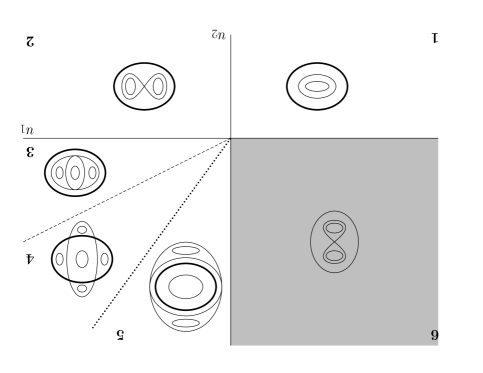
Figure 1: Bifurcation diagram in case $A-3C<A-C<0$ and $\delta<0$.

In this case the deformation $F$ becomes

$$\mathcal{F}(x,y)=-x^{4}+\mu x^{2}y^{2}-y^{4}+u_{1}x^{2}+u_{2}y^{2}+u_{3}x^{2}y^{2}.$$ (51)

The critical points of the planar system are therefore given by (44)–(45) with $\epsilon_{1}=\epsilon_{2}=-1$. The fixed points

$$\left(\pm\sqrt{\frac{u_{1}}{2}},0\right),\quad\left(0,\pm\sqrt{\frac{u_{2}}{2}}\right)$$ (52)

bifurcate from the origin when $u_{1}=0$ and $u_{2}=0$. These critical values of the unfolding parameters respectively determine the bifurcation curves (4) and (4). For $C>0$ and $\delta\leq 0$, these critical values correspond to physical acceptable values if respectively $B>2(A-3C)$ and $B>2(A-C)$. Furthermore, for $\mathcal{E}\approx 0$, both $u_{1}$ and $u_{2}$ are negative and $\mathcal{E}_{1I}<\mathcal{E}_{1L}$. Thus, the bifurcations of fixed points (52) occur according to the diagram given in fig.1, from frame $1$ to $3$. The gray zone corresponds to not acceptable values of the parameters. Concerning the critical points

$$\left(\pm\frac{\sqrt{u_{1}+\frac{\alpha(-\alpha u_{1}-2u_{2})}{-4+\alpha^{2}}}}{\sqrt{2}},\pm\frac{\sqrt{-\alpha u_{1}-2u_{2}}}{\sqrt{-4+\alpha^{2}}}\right),$$ (53)

they determine the bifurcation lines (respectively, the dashed and dotted lines in fig.1)

$$\alpha u_{2}=-2u_{1},\;2u_{2}=-\alpha u_{1}.$$ (54)

The expressions of these critical curves in the $(\delta,\mathcal{E})$ plane are given in (4) and (4).

Remark 6.

The reduced system comes from a normalization procedure truncated to the fourth order in $\epsilon$, in which both $\mathcal{E}$ and $\delta$ are assumed to be of second order. Therefore, in the computation of (4) and (4) from (54) we retain in $\alpha$ only terms $O(|\mathcal{E},\delta|)$, since $\alpha$ has to multiply $x^{2}y^{2}$ which is a fourth order term.

The critical curves (4) and (4) correspond to acceptable values for $B>2(C-A)$ and $B>2(3C-A)$. However, a little computer algebra shows that the critical points (53) fall on the singular circle (18) (frame $4$ in fig.1; the marked circle represents the singular circle), therefore in correspondence of these points the coordinate transformation (16) is not invertible. On the other hand, the fixed points (52) could fall on the limit circle, too. At first order in the deformation parameters, this happens for

$$\frac{u_{1}}{\sqrt{3C-A}}=4\mathcal{E},\;\frac{u_{2}}{\sqrt{C-A}}=4\mathcal{E}.$$ (55)

Solving equations (55) gives the first order term in the detuning parameter of expressions (4) and (4). This suggests that the critical curves (4) and (4) do not determine the bifurcation of new fixed points for the reduced system defined by (15), but rather the disappearance of fixed points (52). To verify this statement, we operate a different planar reduction, according to

$$\left\{\begin{array}[]{ll}x^{\prime}=&\sqrt{2(\mathcal{E}-J)}\cos\psi,\\ y^{\prime}=&\sqrt{2(\mathcal{E}-J)}\sin\psi.\end{array}\right.$$ (56)

In these coordinates the singularity at $J_{2}=0$ is removed and we have a singular circle for $J_{1}=0$. Proceeding as in the previous section we get the universal deformation

$$\mathcal{F}^{\prime}(x^{\prime},y^{\prime})=-x^{\prime 4}+(\mu+u^{\prime}_{3})x^{\prime 2}y^{2}-y^{\prime 4}+u_{1}^{\prime}x^{\prime 2}+u_{2}^{\prime}y^{\prime 2},$$ (57)

where the expressions of the deformation parameters are still determined by proposition 3, but the values of coefficients $a_{i}$ and parameters $b_{i}$ change in view of (56). They are listed in appendix B.

The bifurcation diagram of (57) in the $(u_{1}^{\prime},u_{2}^{\prime})$ plane is still given by fig.1. However, since both $u_{1}^{\prime}$ and $u_{2}^{\prime}$ turn out to be positive for $\delta\leq 0$ and $\mathcal{E}\approx 0$, in the $(u_{1}^{\prime},u_{2}^{\prime})$ plane the bifurcation diagram should be read clockwise from $3$ to $1$. Solving $u_{1}^{\prime}=0$ and $u_{2}^{\prime}=0$ we find the critical curves (4) and (4), which therefore must determine the disappearance of fixed points (52) for the reduced Hamiltonian (15), as we claimed.

Remark 7.

The bifurcation analysis of the reduced system has been performed by assuming $C>0$. For $C<0$ the bifurcation diagram of the germ (43) remains the same given in fig.1. However, since the distinguished parameter must be non-negative and now we have $\mathcal{E}_{1L}<\mathcal{E}_{1I}$, the physical unacceptable zone would be given by panel $2$ and the diagram should be read clockwise starting from frame $1$.

Finally, we obtain the following proposition (here and in the following we denote with $(kK),k=1,2,K=I,i,L,\ell$, a given bifurcation: the digit 1 or 2 denotes the normal mode from (to) which the fixed point originates (or annihilates); the letter denotes the bifurcating family ($I$, inclined, stable; $i$, unstable; $L$, loop, stable; $\ell$, unstable).

Proposition 5.

Let us consider the $1$DOF system $\mathcal{K}$ defined by (15), with $C\neq 0$, $A-3C<0$, $A-C<0$ and non-positive detuning parameter $\delta$. For sufficiently small values of $|\delta|$ the following statements hold:

For $C>0$,

i) if $B>2(A-3C)$: a pitchfork bifurcation (a pair of stable fixed points) appears at

$$\mathcal{E}=\mathcal{E}_{1I}\;\;(1I);$$ (58)

ii) if $B>2(A-C)$: a second pitchfork bifurcation (a pair of unstable fixed points) appears at

$$\mathcal{E}=\mathcal{E}_{1L}\;\;(1\ell);$$ (59)

iii) if $B>2(C-A)$: anti-pitchfork bifurcation (the pair of unstable fixed points disappears) at

$$\mathcal{E}=\mathcal{E}_{2L}\;\;(2\ell);$$ (60)

iv) if $B>2(3C-A)$: a second anti-pitchfork bifurcation (the pair of stable fixed points disappears) at

$$\mathcal{E}=\mathcal{E}_{2I}\;\;(2I);$$ (61)

For $C<0$ the bifurcations listed above occur, if the corresponding conditions on $B$ are satisfied, but in the different sequence given by $(1L)-(1i)-(2i)-(2L)$.

5.1.2 $\epsilon_{1}=\epsilon_{2}=1$

The case $\epsilon_{1}=\epsilon_{2}=1$ follows similarly through the bifurcation analysis of

$$-\mathcal{F}(x,y)=x^{4}+(\tilde{\mu}+\tilde{u}_{3})x^{2}y^{2}+y^{4}+\tilde{u}_{1}x^{2}+\tilde{u}_{2}y^{2}$$

where $\tilde{\mu}=-\mu$, $\tilde{u}_{i}=-u_{i}$, for $i=1,2,3$. We attain the following proposition:

Proposition 6.

Let us consider the $1$DOF system defined by $\mathcal{K}$, with non-positive and sufficiently small detuning parameter, $C\neq 0$, $A-3C>0$ and $A-C>0$.

If $C>0$ and conditions on $B$ are satisfied in order to give positive values for the energy thresholds, the full bifurcation sequence is given by $(2L)-(2i)-(1i)-(1L)$;

if $C<0$ and conditions on $B$ are satisfied in order to give positive values for the energy thresholds, the full bifurcation sequence is given by $(2I)-(2\ell)-(1\ell)-(1I)$.

5.2 $\epsilon_{1}\epsilon_{2}=-1$

5.2.1 $\epsilon_{1}=-\epsilon_{2}=-1$

This case corresponds to $A-3C<0$ and $A-C>0$ and the versal unfolding $F$ turns into

$$\mathcal{G}(x,y)=-x^{4}+(\mu+u_{3})x^{2}y^{2}+y^{4}+u_{1}x^{2}+u_{2}y^{2}$$ (62)

To fix the ideas, let us assume that $A-2C<0$ so that $\mu<0$. With $\alpha=\mu+u_{3}$, the critical points of (62) are then given by $(0,0)$ and

$$\left(\pm\sqrt{\frac{u_{1}}{2}},0\right),\;\;\left(0,\pm\sqrt{\frac{-u_{2}}{2}}\right),$$ (63)

$$\left(\pm\frac{\sqrt{u_{1}+\frac{\alpha(-\alpha u_{1}-2u_{2})}{4+\alpha^{2}}}}{\sqrt{2}},\pm\frac{\sqrt{-\alpha u_{1}-2u_{2}}}{\sqrt{4+\alpha^{2}}}\right).$$ (64)

As we can see in fig.2, the bifurcation diagram of the system is now quite different from the previous one. Again, we are interested in finding bifurcation curves in the $(\delta,\mathcal{E})$ plane for the one degree of freedom system defined by (15). Thus, we limit ourselves to consider what happens inside the singular circle (18), which is marked with a darker line in fig.2. For $\delta\leq 0$ and small values of the distinguished parameter, we have $u_{1}$ and $u_{2}$ both negative. The physical unacceptable zone is now given by frame $7$. Thus, the bifurcation sequence has to be read counter-clockwise starting from frame $1$. Therefore the planar system exhibits the first bifurcation at $u_{1}=0$. The corresponding bifurcation for the $1$DOF system defined by (15) occurs for $\mathcal{E}=\mathcal{E}_{1I}$, which is acceptable only if $B>2(A-3C)$. In frame $3$ we see the appearance of two stable fixed points inside and four unstable points on the singular circle. By using coordinate transformation (56), we can easily check that, if $B>2(C-A)$, the corresponding threshold value for the distinguished parameter is given by (4) and determines the bifurcation of two stable fixed point for $\mathcal{K}$. For

$$u_{2}=-\frac{1}{2}\left(\alpha+\sqrt{\alpha^{2}+4}\right)u_{1}$$ (65)

(marked line in fig.2 separating panels $3$ and $4$) a global bifurcation occurs. The corresponding threshold value for the distinguished parameter is given by

$$\mathcal{E}=\mathcal{E}_{GB}\doteq-\frac{\delta}{2B}+O(\delta^{2})$$ (66)

which is acceptable if $B>0$. Notice that since $\alpha$ multiplies a fourth order term, we can consider (65) only up to the first order in $|\delta,\mathcal{E}|$, cfr remark 6. Therefore, we are able to compute the critical curve (66) only to the first order in the detuning parameter. Then, if $B>2(A-C)$, we can pass through $u_{2}=0$ for $\mathcal{E}=\mathcal{E}_{1L}$ and if $B>2(3C-A)$ a further bifurcation occurs when passing through $u_{1}=0$; the corresponding threshold value for the distinguished parameter is given by (4).

The case $\mu>0$ follows similarly through the bifurcation analysis of

$$-\mathcal{G}(y,x)=-x^{4}+(\tilde{\mu}+\tilde{u}_{3})x^{2}y^{2}+y^{4}+\tilde{u}_{1}x^{2}+\tilde{u}_{2}y^{2}$$

where $\tilde{\mu}=-\mu<0$, $\tilde{u}_{j}=-u_{j}$ for $j=1,2,3$. Finally we have the following proposition:

Proposition 7.

Let us consider the $1$DOF system $\mathcal{K}$ defined by (15) with non-positive and sufficiently small detuning parameter, $C\neq 0$, $A-3C<0$ and $A-C>0$:

For $A-2C<0<A-C$, if conditions on $B$ are satisfied in order to get positive values of the energy thresholds, bifurcations occur along the curves (4)-(4) in the sequence $(1I)-(2L)-(1L)-(2I)$. Furthermore, a global bifurcation might occur between $(2L)$ and $(1L)$ if $B>0$ at

$$\mathcal{E}=\mathcal{E}_{GB}\;\;(GB)$$ (67)

with $\mathcal{E}_{2L}<\mathcal{E}_{GB}<\mathcal{E}_{1L}$.

For $0<A-2C<A-C$, if conditions on $B$ are satisfied in order to give positive values for the energy thresholds, the full bifurcation sequence is given by $(2L)-(1I)-(GB)-(2I)-(1L)$.

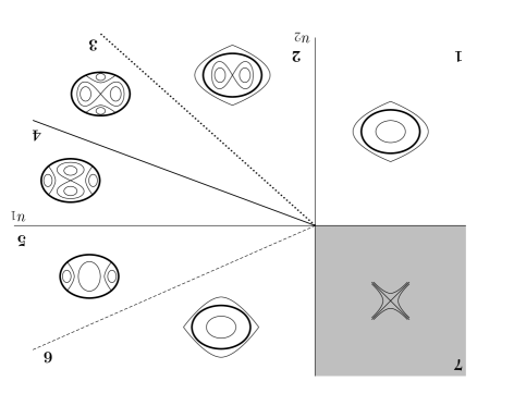
Figure 2: Bifurcation diagram for $A-2C<0<A-C$ and $\delta<0$.

5.2.2 The degenerate case $A=3C$

It remains to analyze the case $\mu=0$, corresponding to the central singularity $y^{4}-x^{4}$. In this case (43) turns into

$$\mathcal{F}(x,y)=-x^{4}+y^{4}+u_{1}x^{2}+u_{2}y^{2}+u_{3}x^{2}y^{2}.$$ (68)

The critical points remain the same given in (63) and (64), but we now have $\alpha=u_{3}$. The bifurcation curves are therefore given by

$$u_{1}=0,\;\;\;\;\;u_{2}=0$$ (69)

and

$$2u_{1} = u_{3}u_{2},$$ (70)

$$2u_{2} = -u_{1}u_{3}.$$ (71)

Solving (69), we find the critical values $\mathcal{E}=\mathcal{E}_{1I}$ and $\mathcal{E}=\mathcal{E}_{1L}$, which respectively turns out to satisfy also (70) and (71). Thus, we get

$$\mathcal{E}_{1I}=\mathcal{E}_{2L}\;\;\;\;\hbox{and}\;\;\;\;\mathcal{E}_{2I}=\mathcal{E}_{1L}.$$ (72)

For the $1$DOF system defined by (15), this implies that the critical points in (63) appear and disappear simultaneously. Furthermore, a global bifurcation occurs for

$$u_{2}=-\frac{1}{2}\left(u_{3}+\sqrt{u_{3}^{2}+4}\right)u_{1}$$ (73)

giving the critical curve (66). Summarizing, the following proposition holds:

Proposition 8.

In the $1$DOF system $\mathcal{K}$ defined by (15), for $A=2C>0$ and non-positive sufficiently small values of the detuning parameter, we have

i) if $B>-2C$ two pitchfork bifurcations occur concurrently (two pairs of stable fixed points appear) at

$$\mathcal{E}=\mathcal{E}_{1I}=\mathcal{E}_{2L};$$

ii) if $B>0$ a global bifurcation occurs at

$$\mathcal{E}=\mathcal{E}_{GB};$$

iii) if $B>2C$ two anti-pitchfork bifurcations occur concurrently (the two pairs of stable fixed points disappear) at

$$\mathcal{E}=\mathcal{E}_{1L}=\mathcal{E}_{2I}.$$

5.2.3 $\epsilon_{1}=-\epsilon_{2}=1$

This last sub-case (treated in [7] as a realization of the $\mathbb{Z}_{2}$-symmetric 1:1 resonance in the “spring-pendulum”) follows similarly through the bifurcation analysis of

$$-{\mathcal{G}}(x,y)=x^{4}+(\tilde{\mu}+\tilde{u}_{3})x^{2}y^{2}-y^{4}+\tilde{u}_{1}x^{2}+\tilde{u}_{2}y^{2}$$

with $\tilde{\mu}=-\mu$, $\tilde{u}_{i}=-u_{i}$, for $i=1,2,3$. Therefore, the following proposition holds:

Proposition 9.

Let us consider the $1$DOF system $\mathcal{K}$ defined by (15), with $C\neq 0$, $A-3C>0$ and $A-C<0$. For non-positive and sufficiently small detuning parameter, bifurcations might occur along the curves (4)–(4) and (66) in agreement with the statements of propositions 5–8. If conditions on $B$ are satisfied in order to give positive values for the energy thresholds,

for $A-2C<0<A-3C$, the full bifurcation sequence is given by $(1L)-(2I)-(GB)-(1I)-(2L)$;

for $0<A-2C<A-3C$ it is given by $(2I)-(1L)-(GB)-(2L)-(1I)$;

for $A=2C$ bifurcations occur according to the statements of proposition 8, but they are reached in the sequence $(1L)-(GB)-(1I)$.

6 Implications for the original system

According to these results, with the versal deformation of this resonance, we know number and nature of the critical points. Including higher orders may shift the positions of the equilibria – and may be essential for quantitative uses – but will not alter their number or stability. The isolated equilibria of the $1$DOF system defined by (15) correspond to relative equilibria for the original system (1) [19, 33]. Of course, the results obtained are limited to low energies, in the neighbourhood of a central equilibrium, but extend to the original system defined by Hamiltonian (1). This statement is based on the fact that the difference between the original Hamiltonian and the normal form (namely, the remainder of the normalization) can be considered a perturbation of the normal form itself [28, 32, 39]. This remark implies that the results concerning periodic orbits can be extended, by applying the implicit function theorem, to the original system [29, 31]. On the same ground, iso-energetic KAM theory [1, 21] can be used to infer the existence of invariant tori seen as non-resonant tori of the normal form surviving when perturbed by the remainder.

Since we pushed the normalization up to and including sixth order terms, the critical curves of proposition 5 give quantitative predictions on the bifurcation and stability of these periodic orbits in the $(\delta,\mathcal{E})$-plane up to second order in the detuning parameter (since, we recall, it is assumed to be associate to a term of higher-order in the series expansions).

For the coordinate transformation (16), the origin in the plane is a fixed point for all values of the parameters and represents the periodic orbit $J_{1}=0$, namely the normal mode along the $x_{2}$-axis (the “short-period” one, in the reference case $\delta<0$). Similarly, if the planar reduction is performed via (56), we find that for all values of the parameters, the origin is a fixed point again, but it corresponds in this case to the periodic orbit $J_{2}=0$, that is the normal mode along the $x_{1}$-axis (the “long-period” one). In the previous section we found threshold values for the distinguished parameter, depending on $\delta$ and on the coefficients of the system, which determine the bifurcation of these periodic orbits in general position from the normal modes of the system. However, it would be better to have an expression of the bifurcation curves in the $(\delta,E)$-plane, where $E$ is the “true” energy of the system. On the long-period axial orbit ($J_{2}=0$, $J_{1}=\mathcal{E}$), we have

$$\mathcal{K} = \mathcal{E}(1+\delta)+(2A+B)\mathcal{E}^{2}$$

$$+ \frac{\mathcal{E}^{2}}{18}\left(-136A^{2}\mathcal{E}-136AB\mathcal{E}-34B^{2}\mathcal{E}+45v_{6,0}\mathcal{E}-72A\delta-36B\delta\right).$$

According to the rescaling (8), $E=\omega_{2}\mathcal{K}$, so that equation (LABEL:ks11) can be used to express the physical energy $E$ in terms of $\mathcal{E}$, namely

$$E=\omega_{2}\left[\mathcal{E}(1+\delta)+\left(2A+B\right)\mathcal{E}^{2}\right].$$ (75)

Thus up to second order in $\delta$, for $\mathcal{E}$ satisfying equations (4), (4) and $\delta$ as defined in (6) we obtain the following threshold values

$$E = E_{2I}\doteq-\frac{\omega_{2}}{2(2A+B-6C)}\delta$$

$$- \frac{\left(104A^{2}+104AB+26B^{2}-1024AC-512BC+2136C^{2}+45v_{6,0}-15v_{4,2}\right)\omega_{2}}{48(2A+B-6C)^{3}}\delta^{2}$$

$$E = E_{2L}\doteq-\frac{\omega_{2}}{2(2A+B-2C)}\delta$$

$$+ \frac{\left(104A^{2}+104AB+26B^{2}-320AC-160BC+216C^{2}+45v_{6,0}-3v_{4,2}\right)\omega_{2}}{48(2A+B-2C)^{3}}\delta^{2}$$

for the appearance (disappearance) of respectively inclined and loop orbits from the long-period axial orbit. They correspond to physically acceptable values, at least for small values of $|\delta|$, if

$$2A+B-6C>0,\;\;\;\hbox{ and }\;\;\;2A+B-2C>0.$$ (78)

These conditions are reversed for $\delta>0$. A similar argument gives the threshold values for the bifurcations from the short-period axial orbit. They are given by

$$E = E_{1I}\doteq\frac{\omega_{2}}{2(2A-B-6C)}\delta$$

$$+ \frac{\left(184A^{2}-184AB+46B^{2}-704AC+352BC+456C^{2}+15v_{2,4}-45v_{0,6}\right)\omega_{2}}{48(2A-B-6C)^{3}}\delta^{2}$$

$$E = E_{1L}\doteq\frac{\omega_{2}}{2(2A-B-2C)}\delta$$

$$+ \frac{\left(184A^{2}-184AB+46B^{2}-256AC+128BC+72C^{2}+3v_{2,4}-45v_{0,6}\right)\omega_{2}}{48(2A-B-2C)^{3}}\delta^{2}$$

and correspond to physically acceptable values, at least for small values of the detuning parameter, if

$$2A-B-6C<0,\;\;\;\hbox{ and }\;\;\;2A-B-2C<0.$$ (81)

Finally, the global bifurcation may occur at

$$E=E_{GB}\doteq-\frac{\omega_{2}\delta}{2B}$$ (82)

if

$$B>0.$$ (83)

The bifurcation sequences of the original system depend on the three coefficients $A,B,C$ according to the statements of propositions 5–9 as we have obtained them in the previous section.

Appendix A Normal Forms

A.1 Action-angle–like variables

The terms in the Birkhoff normal form (11) are

$$K_{0} = J_{1}+J_{2},$$ (84)

$$K_{2} = \delta J_{1}+\frac{3}{2}v_{4,0}J_{1}^{2}+\frac{3}{2}v_{0,4}J_{2}^{2}+\frac{1}{2}v_{2,2}J_{1}J_{2}\left[2+\cos(2\phi_{1}-2\phi_{2})\right],$$ (85)

$$K_{4} = -\delta\left[3v_{4,0}J_{1}^{2}-v_{2,2}J_{1}J_{2}\left(2+\cos(2\phi_{1}-2\phi_{2})\right)\right],$$

$$+ \frac{1}{4}\left(10v_{6,0}-17v_{4,0}^{2}\right)J_{1}^{3}+\frac{1}{4}\left(10v_{0,6}-17v_{0,4}^{2}\right)J_{2}^{3}$$

$$+ \frac{1}{4}J_{1}^{2}J_{2}\left(6v_{4,2}-\frac{9}{4}v_{2,2}^{2}-12v_{2,2}v_{4,0}+\left(4v_{4,2}-2v_{2,2}^{2}-5v_{2,2}v_{4,0}\right)\cos(2\phi_{1}-2\phi_{2})\right)$$

$$+ \frac{1}{4}J_{1}J_{2}^{2}\left(6v_{2,4}-\frac{9}{4}v_{2,2}^{2}-12v_{2,2}v_{0,4}+\left(4v_{2,4}-2v_{2,2}^{2}-5v_{2,2}v_{0,4}\right)\cos(2\phi_{1}-2\phi_{2})\right).$$

A.2 Variables for the first reduction

With the definitions

$$A=\frac{3}{8}(v_{4,0}+v_{0,4}),\;\;\;B=\frac{3}{4}(v_{4,0}-v_{0,4}),\;\;\;C=\frac{1}{8}v_{2,2},$$ (87)

the polynomials in the reduced normal form (15) are

$$\mathcal{A}_{1}(J;\mathcal{E},\delta) = (2A-B)\mathcal{E}^{2}+\left(-4A+2B+8C\right)\mathcal{E}J$$ (88)

$$+ \delta J+4(A-2C)J^{2}.$$

$$\mathcal{B}_{1}(J;\mathcal{E},\delta) = 4CJ(\mathcal{E}-J).$$ (89)

$$\mathcal{A}_{2}(J;\mathcal{E},\delta) = \frac{1}{9}\left(68AB-68A^{2}-17B^{2}+\frac{45}{2}v_{0,6}\right)\mathcal{E}^{3}-8C\delta\mathcal{E}J$$ (90)

$$+ \left(+\frac{68AB}{3}-\frac{68A^{2}}{3}-\frac{17B^{2}}{3}+32AC-48BC+36C^{2}\right.$$

$$+ \left.\frac{3v_{4,2}}{2}-3v_{2,4}+\frac{15v_{0,6}}{2}\right)\mathcal{E}J^{2}+2(4C-2A-B)\delta J^{2}$$

$$+ \left(32BC+\frac{5v_{6,0}}{2}-\frac{136AB}{9}-\frac{3v_{4,2}}{2}+\frac{3v_{2,4}}{2}-\frac{5v_{0,6}}{2}\right)J^{3}.$$

$$\mathcal{B}_{2}(J;\mathcal{E},\tilde{\delta}) = -4C\delta\mathcal{E}J+\left(\frac{40}{3}AC-20BC+32C^{2}+v_{4,2}-2v_{2,4}\right)\mathcal{E}J^{2}$$ (91)

$$+ 4C\delta J^{2}+\left(\frac{40}{3}BC-v_{4,2}+v_{2,4}\right)J^{3}.$$

Appendix B List of coefficients and parameters

In the deformation (29) of proposition 2, if the planar reduction is performed according to (16), the coefficients $a_{i}$ are the following

$$a_{1} = \frac{12(B-2A+6C)}{\sqrt{|3C-A|}}$$

$$a_{2} = \frac{136A^{2}-136AB+34B^{2}-272AC+136BC-408C^{2}+15v_{2,4}-45v_{0,6}}{12\sqrt{|3C-A|}}$$

$$a_{3} = \frac{12(B-2A+2C)}{\sqrt{|C-A|}}$$

$$a_{4} = \frac{136A^{2}-136AB+34B^{2}-112AC+56BC-24C^{2}+3v_{2,4}-45v_{0,6}}{12\sqrt{|C-A|}}$$

$$a_{5} = \frac{1}{288(A-3C)^{2}}(1632A^{3}-544A^{2}(2B+15C)+2A(68B^{2}+3264BC$$

$$+ 9(272C^{2}-5(v_{6,0}+v_{4,2}-3v_{2,4}+5v_{0,6})))$$

$$+ 3(-136B^{2}C-3B(1088C^{2}-5(v_{6,0}-v_{4,2}+v_{2,4}-v_{0,6}))$$

$$+ 18C(272C^{2}+5(v_{6,0}+v_{4,2}-3v_{2,4}+5v_{0,6}))))$$

$$a_{6} = \frac{1}{\left(144|C-A|^{3/2}|3C-A|^{3/2}\right)}\left[-1632A^{4}+64A^{3}(17B+138C)\right.$$

$$- 2A^{2}\left(68B^{2}+3328BC+9\left(640C^{2}-5v_{6,0}-3v_{4,2}+9v_{2,4}-25v_{0,6}\right)\right)$$

$$+ A(512B^{2}C-72C(48C^{2}+5v_{6,0}+2v_{4,2}-8v_{2,4}+25v_{0,6})$$

$$+ B(12608C^{2}-45v_{6,0}+27v_{4,2}-27v_{2,4}+45v_{0,6}))$$

$$- 6C(52B^{2}C+B(1216C^{2}-15v_{6,0}+6v_{4,2}-6v_{2,4}+15v_{0,6})$$

$$- 3C(432C^{2}+5v_{6,0}+7v_{4,2}-25v_{2,4}+85v_{0,6}))]$$

$$a_{7} = \frac{1}{288(A-C)^{2}}\left(1632A^{3}+32A^{2}(34B-93C)\right.$$

$$+ 2A\left(68B^{2}-1216BC+528C^{2}-225v_{6,0}+27v_{4,2}-9v_{2,4}-45v_{0,6}\right)$$

$$+ 3\left(-24B^{2}C+B\left(448C^{2}+3(5v_{6,0}-v_{4,2}+v_{2,4}-5v_{0,6})\right)\right.$$

$$+ \left.\left.6C\left(16C^{2}+25v_{6,0}-3v_{4,2}+v_{2,4}+5v_{0,6}\right)\right)\right).$$

The parameters $b_{i}$ have the following expressions

$$b_{1} = -\frac{6C\delta}{\sqrt{|3C-A|}}$$

$$b_{2} = \frac{\delta}{2\sqrt{|3C-A|}}$$

$$b_{3} = -\frac{2C\delta}{\sqrt{|C-A|}}$$

$$b_{4} = \frac{\delta}{2\sqrt{|C-A|}}$$

$$b_{5} = \frac{\left(576A^{2}+16AB-3456AC-48BC+5184C^{2}+45(v_{6,0}-v_{4,2}+v_{2,4}-v_{0,6})\right)\delta}{576(A-3C)^{2}}$$

$$b_{6} = \left(-576A^{3}-16A^{2}B+3456A^{2}C+32ABC-6336AC^{2}\right.$$

$$+ 48BC^{2}+3456C^{3}-45Av_{6,0}+90Cv_{6,0}+27Av_{4,2}-36Cv_{4,2}-27Av_{2,4}+36Cv_{2,4}$$

$$+ 45Av_{0,6}-90Cv_{0,6})\frac{\delta}{288|C-A|^{3/2}|3C-A|^{3/2}}$$

$$b_{7} = \frac{\left(576A^{2}+16A(B-72C)+48BC+9\left(64C^{2}+5v_{6,0}-v_{4,2}+v_{2,4}-5v_{0,6}\right)\right)\delta}{576(A-C)^{2}}.$$

If the planar reduction is performed according to (56) the previous coefficients and parameters turn into

$$a_{1} = -\frac{12(B+2A-6C)}{\sqrt{|3C-A|}}$$

$$a_{2} = \frac{136A^{2}+136AB+34B^{2}-272AC-136BC-408C^{2}+15v_{4,2}-45v_{6,0}}{12\sqrt{|3C-A|}}$$

$$a_{3} = -\frac{12(B+2A-2C)}{\sqrt{|C-A|}}$$

$$a_{4} = \frac{136A^{2}+136AB+34B^{2}-112AC+56BC-24C^{2}+3v_{4,2}-45v_{6,0}}{12\sqrt{|C-A|}}$$

$$a_{5} = \frac{1}{288(A-3C)^{2}}(1632A^{3}+544A^{2}(2B-15C)+2A(68B^{2}-3264BC$$

$$+ 9(272C^{2}-5(v_{6,0}-3v_{4,2}+v_{2,4}-v_{0,6})))$$

$$+ 3(-136B^{2}C+3B(1088C^{2}+5(v_{6,0}-v_{4,2}+v_{2,4}-v_{0,6}))$$

$$+ 18C(272C^{2}+5(v_{6,0}-3v_{4,2}+v_{2,4}+v_{0,6}))))$$

$$a_{6} = \frac{1}{\left(144|C-A|^{3/2}|3C-A|^{3/2}\right)}\left[-1632A^{4}-64A^{3}(17B-138C)\right.$$

$$- 2A^{2}\left(68B^{2}-3328BC+9\left(640C^{2}-25v_{6,0}+9v_{4,2}-3v_{2,4}-5v_{0,6}\right)\right)$$

$$+ A(512B^{2}C-72C(48C^{2}+25v_{6,0}-8v_{4,2}+2v_{2,4}+5v_{0,6})$$

$$+ B(-12608C^{2}-45v_{6,0}+27v_{4,2}-27v_{2,4}+45v_{0,6}))$$

$$+ 6C(-52B^{2}C+B(1216C^{2}+15v_{6,0}-6v_{4,2}+6v_{2,4}+5v_{0,6})$$

$$+ 3C(432C^{2}+85v_{6,0}-25v_{4,2}+7v_{2,4}+5v_{0,6}))]$$

$$b_{1} = \frac{2(2A+B-3C)\delta}{\sqrt{-A+3C}}$$

$$b_{2} = -\frac{\delta}{2\sqrt{|3C-A|}}$$

$$b_{3} = \frac{2(2A+B-C)\delta}{\sqrt{-A+C}}$$

$$b_{4} = -\frac{\delta}{2\sqrt{|C-A|}}$$

$$b_{5} = \frac{\left(576A^{2}+16AB-3456AC-48BC+5184C^{2}+45(v_{6,0}-v_{4,2}+v_{2,4}-v_{0,6})\right)\delta}{576(A-3C)^{2}}$$

$$b_{6} = \left(-576A^{3}-16A^{2}B+3456A^{2}C+32ABC-6336AC^{2}\right.$$

$$+ 48BC^{2}+3456C^{3}-45Av_{6,0}+90Cv_{6,0}+27Av_{4,2}-36Cv_{4,2}-27Av_{2,4}+36Cv_{2,4}$$

$$+ 45Av_{0,6}-90Cv_{0,6})\frac{\delta}{288|C-A|^{3/2}|3C-A|^{3/2}}$$

$$b_{7} = \frac{\left(576A^{2}+16A(B-72C)+48BC+9\left(64C^{2}+5v_{6,0}-v_{4,2}+v_{2,4}-5v_{0,6}\right)\right)\delta}{576(A-C)^{2}}$$

References

- [1] Arnold, V.I. Small denominators and problems of stability of motion in classical and celestial mechanics, Russ. Math. Surv. 18(6), 85–191 (1963).
- [2] Belmonte, C. Boccaletti, D. & Pucacco, G. On the orbit structure of the logarithmic potential, The Astrophysical Journal 669, 202–217 (2007).
- [3] Binney, J. Resonant excitation of motion perpendicular to galactic planes, Monthly Notices of the Royal Astronomical Society, 196, 455–467 (1981).
- [4] Birkhoff, G. D. Dynamical Systems, 9, American Mathematical Society, Providence, Rhode Island (1927).
- [5] Bosschaert, M. & Hanßmann, H. Bifurcations in Hamiltonian systems with a reflection symmetry, Qual. Theory Dyn. Syst. 12, 67–87 (2013).
- [6] Broer, H.W. Chow, S.N. Kim, Y. & Vegter, G. A normally elliptic Hamiltonian bifurcation, Z. angew. Math. Phys., 44, 389–432 (1993).
- [7] Broer H.W., Lunter G.A. & Vegter G. Equivariant singularity theory with distinguished parameters: Two case studies of resonant Hamiltonian systems, Physica D 112, 64–80 (1998).
- [8] Broer, H.W. Hoveijn, I. Lunter, G.A. & Vegter, G. Resonances in a spring pendulum: algorithms for equivariant singularity theory, Nonlinearity 11, 1569–1605 (1998).
- [9] Broer, H.W. Hoveijn, I. Lunter, G.A. & Vegter, G. Bifurcations in Hamiltonian systems: computing singularites by Gröbner bases, Lecture Notes in Mathematics 1806, Springer-Verlag (2003).
- [10] Cicogna, G. & Gaeta, G. Symmetry and perturbation theory in nonlinear dynamics, Springer-Verlag, Berlin (1999).
- [11] Contopoulos, G. Resonance cases and small divisors in a third integral of motion. I, Astronomical Journal, 68, 763–779 (1963).
- [12] Contopoulos, G. Order and Chaos in Dynamical Astronomy, Springer-Verlag, Berlin (2004).
- [13] Contopoulos, G. & Moutsoulas M. Resonance cases and small divisors in a third integral of motion. III, Astronomical Journal, 71, 687–698 (1966).
- [14] Cotter, C. S. The 1:1 resonance and the Hénon-Heiles family of Hamiltonians, PhD Thesis, University of California at Santa Cruz (1986).
- [15] Cushman, R. H. & Bates, L. M. Global aspects of classical integrable systems, Birkhauser (1997).
- [16] Cushman, R. H. Dullin, H.R. Hanßmann, H. & Schmidt, S. The 1: resonance, Regular and Chaotic Dynamics, 12, 642–663 (2007).
- [17] Cushman, R. H. & Rod, D. L. Reduction of the semi-simple 1:1 resonance, Physica D, 6, 105–112 (1982).
- [18] Deprit, A. The Lissajous transformation. I. Basics., Celestial Mechanics and Dynamical Astronomy 51, 201–225 (1991).
- [19] Deprit, A. & Elipe, A. The Lissajous transformation. II. Normalization., Celestial Mechanics and Dynamical Astronomy 51, 227–250 (1991).
- [20] Duistermaat, J. J. Bifurcation of periodic solutions near equilibrium points of Hamiltonian systems Lecture Notes in Mathematics, 1057, 57–105, Springer-Verlag (1984).
- [21] Ferrer, F. Hanßmann, H. Palacián, J. & Yanguas, P. On perturbed oscillators in 1:1:1 resonance: the case of axially symmetric cubic potentials J. Geom. Phys., 40 320–369 (2002).
- [22] Giorgilli, A. Notes on Exponential Stability of Hamiltonian Systems, Centro di Ricerca Matematica E. De Giorgi, Pisa (2002).
- [23] Golubitsky, M. & Schaeffer, D.G. Singularities and Groups in Bifurcation Theory, 1, Applied Mathematical Sciences, 51, Springer-Verlag, Berlin (1985).
- [24] Golubitsky, M. Stewart, I. & Schaeffer, D.G. Singularities and Groups in Bifurcation Theory, 2, Applied Mathematical Sciences, 69, Springer-Verlag, Berlin (1988).
- [25] Golubitsky, M. Marsden, J.E. Stewart, I. & Dellnitz, M. The constrained Liapunov-Schmidt Procedure and periodic orbits, Fields Institute Communications 4, 81–127 (1995).
- [26] Hanßmann, H. On Hamiltonian bifurcations of invariant tori with a Floquet multiplier , Dynamical Systems, 21, 115–145 (2006).
- [27] Hanßmann, H. Local and Semi-Local Bifurcations in Hamiltonian Dynamical Systems, Lecture Notes in Mathematics 1893, Springer-Verlag (2007).
- [28] Hanßmann, H. & Sommer, B. A degenerate bifurcation in the Hénon-Heiles Family, Celestial Mechanics and Dynamical Astronomy 81, 249–261 (2001).
- [29] Henrard, J. Periodic orbits emanating from a resonant equilibrium, Celestial Mechanics, 1, 437–466 (1969).
- [30] Kas, A. & Schlessinger, M., On the versal deformation of a complex space with an isolated singularity, Math. Ann., 196, 23–29 (1972).
- [31] Kummer, M. On resonant non linearly coupled oscillators with two equal frequencies., Communication in Mathematical Physics, 48, 53–79 (1976).
- [32] Meyer, K.R. Hall, G.R. & Offin, D. Introduction to Hamiltonian dynamical systems and the N body problem, Applied Mathematical Sciences, 90, Springer-Verlag (1985).
- [33] Miller, B. R. The Lissajous transformation. III. Parametric bifurcations., Celestial Mechanics and Dynamical Astronomy 51, 251–270 (1991).
- [34] Marchesiello, A. & Pucacco, G. Relevance of the 1:1 resonance in galactic dynamics, Eur. Phys. J. Plus 126, 104–118 (2011).
- [35] Marchesiello, A. & Pucacco, G. Resonances and bifurcations in systems with elliptical equipotentials, MNRAS 428, 2029–2038 (2013).
- [36] Martinet, J. Singularities of Smooth Functions and Maps, LMS Lecture Note Series, 58, Cambridge University Press, Cambridge, 1982.
- [37] Montaldi, J. Roberts, M & Stewart, I. Existence of nonlinear normal modes of symmetric Hamiltonian systems, Nonlinearity 3, 695–730 (1990).
- [38] Montaldi, J. Roberts, M & Stewart, I. Stability of nonlinear normal modes of symmetric Hamiltonian systems, Nonlinearity 3, 731–772 (1990).
- [39] Sanders, J. A. Verhulst F. and Murdock, J. Averaging Methods in Nonlinear Dynamical Systems, Springer-Verlag, Berlin, Heidelberg (2007).
- [40] van der Meer, J. C. The Hamiltonian Hopf bifurcation, Lecture Notes in Mathematics 1160, Springer-Verlag (1985).
- [41] van der Meer, J. C. Degenerate Hamiltonian Hopf bifurcations, Fields Institute Communications 8, 159–176 (1996).
- [42] van der Meer, J. C. One-parameter versal deformations of symmetric Hamiltonian systems in 1:1 resonance, Int. Journal of Pure and Appl. Math. 53, 547–561 (2009).
- [43] Verhulst, F. Discrete symmetric dynamical systems at the main resonances with applications to axi-symmetric galaxies, Royal Society (London), Philosophical Transactions, Series A, 290, 435–465 (1979).
- [44] de Zeeuw, T. & Merritt, D. Stellar orbits in a triaxial galaxy. I. Orbits in the plane of rotation, The Astrophysical Journal, 267, 571–595 (1983).